Abstract
Effective response to flood events requires high-resolution, frequently updated data on flooded areas for comprehensive flood risk assessments. Unmanned aerial vehicles (UAVs) equipped with conventional camera systems and classification based on orthophotos from photogrammetric postprocessing and artificial intelligence are widely used to detect flooded areas. However, these methods often involve time-intensive pre- and postprocessing steps and fail to incorporate geometric factors such as elevation data and water depths. This study introduces SSegRef2Surf, a novel tool that integrates classified flood raster data with terrain information. SSegRef2Surf refines and optimizes coarse raster classifications by filling shadowed areas and correcting misclassified regions. This tool reduces data requirements for AI training and minimizes postprocessing time, enabling near real-time flood monitoring. All processes necessary for SSegRef2Surf were optimized through sensitivity and accuracy analyses to reduce postprocessing duration to a minimum. A comparison of the SSegRef2Surf results with two-dimensional (2D) numerical model results for a flood event revealed discrepancies in the 2D model, caused by inaccuracies in the underlying terrain data. This comparison showed that 30% of the flooded areas identified in the 2D numerical results were incorrect, while missing areas (11%) were added. This highlights the significant potential of SSegRef2Surf for near real-time flood monitoring and traceability of flood events, as combining UAVs’ high-frequency surveying capabilities with SSegRef2Surf allows for more effective validation and optimization of 2D models.
1. Introduction
The frequency and intensity of flood events (FEs) in Germany and across Europe have significantly increased in recent years [1]. For example, ref. [2] identified rising winter precipitation events through an analysis of temperature and precipitation trends. The rising precipitation trend, combined with human activities such as increasingly sealed surfaces [3] and reshaped river systems by straightening waterways and narrowing flow cross sections, results in intensified peak discharges and accelerated flood waves. To prevent damages caused by these hydraulic events, authorities emphasized the need to relocate dikes, de-seal surfaces, adopt site-appropriate land and forestry practices, and restore rivers to preserve natural environmental resources in the “Guidelines for Forward-Looking Flood Protection” by the Federal/State Working Group on Water (LAWA, [4]). Although different measures have been conducted in recent years, society cannot completely prevent major flood events with certainty [4]. Therefore, it is essential for people to acknowledge that flood events are natural occurrences to which humanity will always be vulnerable [3,5]. This understanding inspired the European Flood Risk Management Directive (EU-FRMD, ger. “Hochwasserrisikomanagement-Richtlinie der Europäischen Gemeinschaft”, EG-HWRM-RL [5]), which aims to guide member states in systematically assessing, mapping, and managing flood risks. Building on this directive, LAWA published the “Guidelines for Forward-Looking Flood Protection” [6], which serve as practical instructions for implementing the EU-FRMD. Further guidelines and recommendations related to flood protection and flood risk management have also been issued. These include guidance on river structure mapping for small- and medium-sized watercourses [7], the development of flood action plans [8], and the preparation of flood management plans [9]. These guidelines provide various planning and analytical foundations that are applied in the management of flood events.
Specific analytical tools have been developed based on the recommendations for creating flood hazard maps outlined in [10] and their updates in [11]. These tools visualize the extent of significant flood events based on hydraulic parameters (typically flow velocity, water depth, and flow vectors) and assess risks to infrastructure. The results of two-dimensional (2D) hydrodynamic numerical models serve as the primary data source for these maps. These maps and models facilitate the analysis of past events to prevent future catastrophes and protect existing infrastructure. The data underlying these maps typically rely on measurements from previous flood events recorded by stream gauging stations. The extent of the flooded areas is often documented only superficially and at large time intervals, which limits the precision of floodplain development assessments and the validation of two-dimensional numerical model results.
Since 2D model results are critical to flood risk assessment, their reliability and accuracy are of immense importance [12]. Input parameters (e.g., discharge) are either derived from rainfall–runoff models or based on statistical parameters based on stream gauging station observations, and the 2D models are calibrated using in situ measurements (flood marks). However, in situ data only represent specific flood events and cannot account for all potential statistical events, which are instead derived through inter- or extrapolation. Discrepancies between model results and in situ measurements during a flood event may arise due to these limitations. During extreme flood events, measurement equipment often fails to provide reliable data. For instance, during the severe flood in July 2021 in the Ahr Valley in Germany, five of the eight stream gauging stations failed due to the intense flow conditions [13], limiting the ability to fully analyze the event.
Ref. [14] highlights the deficit of natural measurement data during flood events and underscores their importance for analyzing flood events.
He also stresses the need for improved baseline data to describe hydrological and hydraulic processes. According to the author of [14], a better understanding of the boundary conditions of a waterbody can significantly improve the accuracy of numerical calculations. He further mentions that the deficit of in situ data “[…] can only be addressed through the preparation and implementation of operational measurement programs for flood events […]” (translated by the author. Original text: “Das große Defizit an Naturmessdaten (z. B. Wasserstand, Durchfluss, Rauheiten, Überschwemmungsflächen, …) im Hochwasserfall lässt sich nur durch die Vorbereitung und Umsetzung von operativen Messprogrammen für den Hochwasserfall lösen”) [14] (p. 30). The authors of [15] reinforce this statement by emphasizing the need for new methods to survey river systems, particularly highlighting the use of fixed-wing unmanned aerial vehicles (UAVs) for capturing flood events, while the authors of [16] discuss the growing demand for well-suited methods to survey flood events with high temporal resolution and accuracy.
For assessing and mapping flood events, different survey methods offer different ways to capture and analyze these events, with notable variations in measurement accuracy and coverage area. It is necessary to analyze the capabilities of current remote sensing methods and systems to effectively map flood events with high accuracy and high spatio-temporal resolution.
Using UAVs with RGB camera systems enables the optical monitoring of flood events in near real-time. While the use of UAVs allows for high mapping intervals and consequently high data densities, the postprocessing is often associated with a very high duration. Pixel-based analyses enable the extraction of water surface information from orthophotos and images. This process involves grouping and classifying individual image pixels based on shared color features, a method referred to as semantic segmentation. AI-supported techniques, such as unsupervised and supervised deep learning, are frequently applied but often demand significant preparatory effort and a large amount of training data [17]. While flood risk maps and flood hazard maps are tools that visually assess flood risks in a preventive manner, there is a need for tools that enable flexible and rapid data collection and postprocessing during a flood event. Such tools are crucial for analyzing the extent of floodplain areas, comprehensively understanding hydraulic processes, decision-making, and implementing measures to mitigate flood-related damage. The SSegRef2Surf (Semantic Segmentation Refinement to create 2D Water Surfaces) tool was developed to enable near real-time mapping of flood events with minimal preprocessing and low data requirements. Classification results from UAV photos are combined with digital elevation models (DEMs) to refine coarsely classified areas and filter out misclassified regions. The necessary processing workflows have been automated and optimized, ensuring efficient utilization of computational resources and facilitating parallel processing. The low preparatory effort and minimal data density requirements allow for its application across a wide range of study areas, enabling quick and straightforward implementation during flood events. This study demonstrates how optimized postprocessing and surveying workflows, combined with the integration of photogrammetry, AI classification, and DEMs, enable high-frequency detection of flood events and how this enhances near real-time flood risk assessment and 2D numerical models.
At the beginning of this study, we introduce the importance of near real-time data in the context of flood events. The summary of commonly used remote sensing methods and systems highlights their potential for detecting flood areas and utilizing the data to identify water surfaces. The advantages and limitations of these systems are discussed in the context of near real-time flood mapping. After defining the study area, the optimized survey process during a flood event in February 2023 and the subsequent data postprocessing are explained. This includes the generation of high-accuracy orthophotos from aerial images through Structure from Motion (SfM) and process optimization, the identification of water surfaces using a coarse classification, and their refinement with SSegRef2Surf. The results demonstrate the impact of the accuracy and optimization processes in achieving a good balance between precision and the duration of data acquisition and postprocessing. We compare our findings with hydraulic numerical results and discuss them in the context of current research. The conclusions highlight future research possibilities, emphasizing scalability and applicability to larger study areas.
1.1. Near Real-Time Risk Assessment
Risk assessment is typically conducted by analyzing the probability of a flood event and its potential negative impact [14]. The risk value is calculated as the product of these two factors. The second input variable, also known as vulnerability, measures exposure, susceptibility, and potential damage during a flood event [14,18]. Vulnerability is defined by the exposure and susceptibility of an object [19] and plays a crucial role in flood risk management and the implementation of measures to prevent severe damage to infrastructure and loss of life. The author of [18] divides vulnerability into two components: technical and social. For the social component, he highlights the anthropogenic response potential, which refers, for example, to the improper implementation of measures during a flood event. As an example of technical vulnerability, he describes the faulty construction of hydraulic structures. To reduce social vulnerability and ensure effective response potential, near real-time data must be available to enable an adequate reaction to flood events.
A lack of datasets with high spatio-temporal resolution has often hindered retrospective analysis of past flood events and highlights the critical importance of such data during an event to implement measures effectively. This lack of datasets shows the need for rapid surveying methods to generate high-density data for assessing flood events [16]. “Near-real-time” is a term frequently used to describe time-efficient analyses. Its precise definition varies in research contexts. For instance, in satellite image analysis [20], “real-time” often refers to rapid postprocessing, where water surfaces can be extracted quickly. Ref. [21] demonstrated near real-time flood mapping by postprocessing SAR imagery in under a minute. However, satellite images are typically collected at daily intervals [22], and data availability also involves delays. Fixed terrestrial measurement units can produce very precise and rapid data. Refs. [23,24,25,26] describe near real-time rockfall monitoring using stationary camera systems to detect changes within seconds, meeting the near real-time criteria. However, such systems lack flexibility due to their fixed locations and require extensive preconditions for data processing, such as deep neural networks trained on extensive datasets (e.g., [23]). The term “near real-time” thus encompasses a wide range of applications. UAVs provide an effective balance between large-area coverage, time efficiency, and high accuracy. Optimized capture and processing workflows can yield results within highly efficient timeframes (<1 h, [27]). This makes UAV-based measurements an effective intermediary between the longer temporal resolution of satellite imaging (days) and the instantaneous data acquisition of stationary units (seconds), making them a valuable approach for capturing near real-time data while facilitating efficient postprocessing.
1.2. State of the Art Remote Sensing Systems
Recent advancements in remote sensing systems offer great potential for surveying hydrological processes [28]. In recent years, numerous measurement instruments and techniques have been applied for environmental monitoring and surveying. These techniques vary in methods, accuracy, survey intervals, and coverage area. Considering these components, selecting and applying an appropriate method for capturing flood events is critical when analyzing specific study areas.
Unmanned aerial vehicles (UAVs) have seen rapid growth in application due to their multidisciplinary capabilities. Combined with RGB camera systems, UAVs can use photogrammetry through the Structure from Motion (SfM) method, which provides cost-effective, efficient, flexible, and high-resolution spatial data [15]. This method has been extensively documented for applications such as monitoring flood events [17,27,29,30,31,32,33]; ice jams [34]; generating digital elevation and surface models (DEMs and DSMs, [35]); and change detection [27,32,36,37,38].
UAV-based Light Detection and Ranging (LiDAR) systems provide direct distance measurements by comparing emitted and reflected laser beams. Like SfM, LiDAR enables various surveying tasks, many of which are described in [37,39,40]. Many LiDAR systems analyze emitted and reflected signals across the full laser spectrum (multi-echo and full waveform [30]). This allows for the categorization of reflections into vegetation, infrastructure, or water surfaces. However, LiDAR is typically more expensive than SfM. Additionally, due to its higher payload and increased battery load, UAV flight times and corresponding coverage areas are reduced compared to the use of standard camera systems.
The availability of satellite data in recent years has opened new possibilities for environmental research, disaster management, and land-use analysis. Programs such as Copernicus (European Space Agency, ESA) and Landsat (NASA and USGS) provide high-resolution and continuous data to the public, enabling real-time monitoring of climate changes and environmental disasters, as well as detailed analyses of urban development, agricultural optimization, and sustainable resource management. Synthetic Aperture Radar (SAR) satellites like Sentinel-1 have the advantage of capturing data even at night or under cloudy conditions [41,42], while optical sensors are limited by such factors [43]. Smooth water surfaces act as mirrors for electromagnetic waves, appearing black in satellite images [44]. This enables the classification and categorization of data [45]. Satellite data archives spanning long periods allow retrospective analysis of past flood events.
1.3. Identification of Water Surface
The detection of water bodies varies depending on the remote sensing system. Systems that compare emitted and reflected signals take advantage of water’s ability to scatter or strongly reflect these signals. In flooded areas, the system thus receives weak or almost no signals. Using single-image thresholding, such areas can be identified based on set thresholds. However, other surfaces may also exhibit similar reflection properties, making it difficult to always classify them as water bodies [22].
Another effective method for identifying flooded areas is change detection (CD). This involves comparing an image taken during a flood event (co-event image) with an image taken before the event (pre-event image) [22]. Changes in pixel values indicate flooded areas. This method can be extended to time series analysis, where the “normal state” is defined over a longer time series, and deviations are statistically evaluated [22].
Image analysis using artificial intelligence (AI)—both supervised and unsupervised– has been widely studied [17,33,46,47,48]. However, according to the authors of [49] (p. 15), supervised methods have the disadvantage that, compared to traditional thresholding methods, they “[…] are driven by a huge amount of specific (annotated) data to generate plausible results”. Additionally, the variability in image data, particularly in long time series with changing light and vegetation conditions, complicates the training process and increases the effort.
2. Study Area and Flood Event of February 2023
The Laufer Muehle area and its location were previously described in [27,50]. The study area encompasses approximately 0.4 km2 along the Aisch River in Bavaria, near Nuremberg. During a small flood event in February 2023, this area was surveyed using UAV technology and Structure from Motion (SfM) photogrammetry (Figure 1).
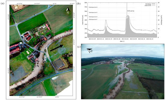
Figure 1.
Laufer Muehle during the flood event (FE) on 3 February 2023. (a) Orthophoto of UAV SfM survey; localization and viewing direction of (c); (b) water level and discharge during FE (data retrieved from [51]); (c) photo of the flooded area with a view from Laufer Muehle in eastern direction.
3. Materials and Methods
3.1. Orthophoto Generation and Optimization
The study area was surveyed using a DJI Phantom 4 RTK drone with real-time kinematic (RTK) and SAPOS [52]. We used Agisoft Metashape 1.8.4 for photogrammetric reconstruction of aerial imagery through Structure from Motion (SfM). The accuracy parameters for SfM postprocessing result from studies in [27,50], upon which the present investigations build. These studies evaluated survey data using georeferenced ground control points (GCPs). Various survey parameter combinations were tested to analyze the relationship between survey duration and the accuracy of point cloud data of SfM postprocessing. The analysis showed that the parameters from Mission M17 provided the most effective balance. Table 1 shows the flight parameters of the missions (Ms) conducted in double grid (DG) and normal grid (NG) flight modes.

Table 1.
Mission parameters of the surveys used for accuracy assessment.
Previous investigations primarily focused on three-dimensional change detection (CD) in the study area and comparisons with 2D model results (100-year flood). The change detection results were visualized using orthophotos, which were generated in a postprocessing process parallel to the CD process. The processes to analyze and visualize changes were implemented into a change detection tool (CDT) [50]. The automated workflow for near real-time flood analysis developed in this study was integrated into the CDT, enhancing its capabilities.
As discussed in [50], the orthophoto generation process dominated the total CDT workflow duration. Orthophotos were used solely for visualization in the change detection process, and their positional accuracy received only peripheral attention. One of the primary goals of the current investigations was to enable near real-time mapping of flood events. This necessitated optimizing the orthophoto generation process and performing accuracy analyses. Reducing the duration of orthophoto generation directly decreases the overall CDT workflow time, making this optimization doubly critical.
The horizontal position accuracy of orthophotos from different missions was the focus of the accuracy analysis. Elevation data for the floodplain were derived from a DEM. Orthophotos were generated from imagery acquired during surveys in September 2022 (no active flood event) using SfM and a high-performance cluster (HPC). Ref. [50] provides a detailed account of the workflow optimizations focused on processor utilization.
The key calculation steps for generating an orthophoto using SfM and Agisoft Metashape are outlined as follows:
- Match Photos (accuracy parameter: Match Photos Downscale, MPD)
- Build Depth Maps (accuracy parameter: Build Depth Maps Downscale, BDD)
- Build Model (Mesh generation; Quality parameter: face count)
- Build Orthomosaic (Orthophoto generation process; Quality parameter: pixel size)
Parameters for Steps 3 and 4 influence only the data density of the orthophoto and not the accuracy of computational results. Thus, these parameters were kept constant at face count = high and pixel size = 0.05 m. Parameters for Steps 1 and 2 were varied to assess their impact on the accuracy of the orthophotos (Table 2).
Table 2.
Accuracy settings (S) (Match Photos Downscale, MPD; Build Depth Maps Downscale, BDD) used for precision analysis of the orthophotos [53].
Data from missions M2, M5, M14, M16, and M17 were analyzed to identify mission parameters with an acceptable ratio between accuracy and survey duration. (missions defined in [27] and parameters described in Section 4.1). We selected these missions based on the following considerations:
- M2: Featured the highest accuracy due to its survey parameters (flight altitude 50 m, ground sampling distance (GSD) = 1.37 cm/pixel, double grid (DG) flight mode). However, its high postprocessing duration made it unsuitable for near real-time analyses in [27].
- M5: Selected as a representative dataset for GSD = 2.19 cm/pixel (flight altitude 80 m). It exhibited a shorter flight duration compared to M2 due to the normal grid (NG) flight mode.
- M14, M16, M17: GSD = 3.01 cm/pixel (120 m flight altitude). M14 represented a dataset with a very short flight duration and a low number of images. M17, highlighted in [27] as the mission with the best acquisition parameters for three-dimensional change detection, underwent further analysis. M16 featured nearly identical parameters to M17 but utilized the normal grid flight mode, which reduced the flight duration and the number of images compared to the double grid flight mode.
The accuracy of orthophotos was evaluated using five postprocessing accuracy settings for the variables MPD and BDD. Key and tie points were unrestricted (value = 0, no limit). Table 2 shows the settings, following terminology from the Agisoft Metashape manual [53].
The investigation focused on determining which postprocessing settings achieve sufficient accuracy when comparing the positions of ground control points (GCPs). The GCPs were measured using a GNSS rover with RTK. The results of this analysis are presented and discussed in Section 4.1.
3.2. SSegRef2Surf—Semantic Water Surface Segmentation and Refinement
Deriving the geometric properties of water surfaces from three-dimensional datasets poses significant challenges due to water movement (caused by flow dynamics or wind) and reflective surface properties, often resulting in inaccurate outcomes. Pixel-based analyses enable the extraction of water surface information from orthophotos and images. This involves grouping and classifying individual image pixels based on shared (color) features, a process referred to as semantic segmentation. Various segmentation methods are available, ranging from traditional approaches to advanced AI-supported techniques. Regardless of the chosen classification method, certain considerations must be addressed:
- A substantial volume of training data is required to ensure accurate classification.
- Variations in time of day, season, and weather conditions affect light and shadow, causing temporal images to differ in color spectrum.
- As a result, algorithms must be tailored to the specific local conditions of the study area, making accurate results highly resource-intensive.
The authors of [17] (p. 11) state that “Training a deep CNN [convolutional neural network] from scratch with a small dataset is not always advisable due to poor classification results and overfitting”. However, they report achieving satisfactory classification results in their study “[…] even though only one hundred UAV images were available for training” [17] (p. 11). This underscores that conventional analysis methods require a high density of data to achieve sufficiently accurate results. Despite favorable outcomes, limitations persist; for example, shadows and canopy cover often make specific areas in images unanalyzable. The authors of [17] emphasize the necessity of supplementary 3D analyses to fill these gaps. This demonstrates the need for alternative methods capable of deriving water surfaces in regions with sparse data availability, limited prior knowledge, and minimal preprocessing to facilitate flood event analysis. To address this, SSegRef2Surf (Semantic Segmentation Refinement to create 2D Water Surfaces) was developed. This tool refines coarsely classified water surface data from RGB orthophotos by correlating these data with a DEM, thereby improving accuracy and filling missing areas. SSegRef2Surf allows for the correction of misclassified areas through refinement and the addition of missing regions to the classification results. While semantic segmentation using AI remains essential for extracting water surfaces, SSegRef2Surf offers flexibility by accommodating a wide range of classified datasets. It only requires a geometrically processed raster file (TIFF) as input.
In these investigations, an orthophoto from the flood event described in Section 2 (February 2023) was classified into the categories “water” (value 1) and “no water” (value 0) using a support vector machine (SVM). This method defines a hyperplane that maximizes the margin distance between points of different classes [30]. We used this method because it integrates well into automated processes using Python v. 2.7 and the ArcPy library.
The supervised learning and execution of the SVM were conducted using ArcGIS Pro v. 3.3.1. Different regions of the orthophoto were classified into “water” and “no water” classes using shapefiles. The classification boundaries were broadly delineated based on visual features without distinguishing individual components (e.g., buildings, roads, or vegetation). After this process, the trained SVM was applied to classify the orthophotos. Figure 2 illustrates the defined boundaries and the resulting water surface classification.
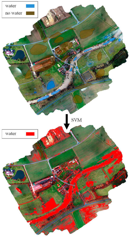
Figure 2.
Classification input (top image) and resulting output (bottom image) from the SVM classification.
The following explanation describes the refinement process of classified raster data using the SSegRef2Surf tool. The refinement process is described based on the input parameters, which are defined and initiated via the CDT user interface (Section 3.4).
The water axis of the river (shapefile) is simplified in the first step of the process. This refinement ensures that the cross sections, which are created in a following step, are oriented perpendicular to the overall course of the river, even in strongly curved and meandering river courses. The degree of simplification depends on the course of the river and is defined by the input value Simplify water axis distance. The simplified water axis is divided into anchor points, spaced by a defined distance (Distance between cross sections, value “d”). A cross section is generated perpendicular to the water axis with a definable length (Length per cross section) at each anchor point. It is important to choose the length so that the cross sections extend beyond the floodplain on both sides.
Measurement points are defined along the cross sections at intervals specified by the Distance between points along cross section parameter. All subsequent calculation steps are carried out at these points.
In the output file generated from the previous classification process (Classified file, which in this study, is the result of the SVM classification), the regions identified as water need to be determined. Using the Water value column name parameter (the column in the output file representing water values) and the Water value parameter (e.g., 1 for water, 0 for no water), water areas located within a specified distance (Distance polygon to water axis) from the simplified water axis are selected. This selection ensures the exclusion of incorrectly identified water areas and those not directly connected to the river.
For each measurement point on the cross sections, it is checked whether the point lies within the water area. A comparison with the digital elevation model (DEM) is made for the measurement points in the water area, and the elevation at each measurement point is determined. The highest value for each cross section is chosen as the representative value for the entire cross section and transferred accordingly. This procedure assumes a constant water surface elevation across each cross-sectional profile. With an appropriate resolution of the DEM and the measurement grid, the intersection between the water surface and the terrain (bankline) is approximately captured.
In the next step, the cross-sectional profiles are transferred into a digital surface model (water-DSM), which represents the extrapolated water surface elevation. For data export, the coordinate system (Spatial reference) and cell size (Export cell size) of the exported raster file are specified. Intersecting the water-DSM with the DEM leads to the identification of areas where the water-DSM elevation exceeds the terrain elevation (DEM). These areas represent flooded areas.
The water depth of the identified flooded areas results from subtracting the terrain elevation (DEM) from the water surface elevation (water-DSM). Figure 3 visualizes the geometric parameters of the SSegRef2Surf tool.
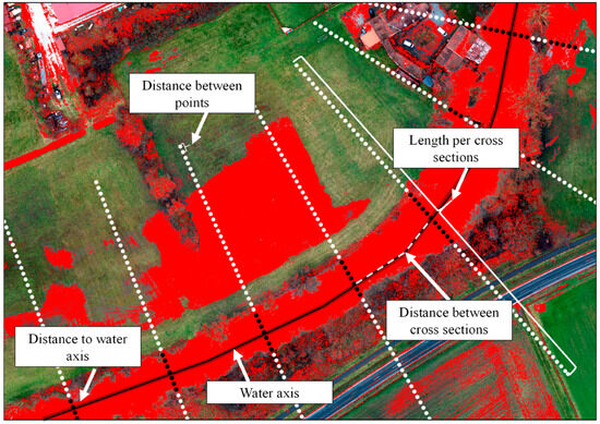
Figure 3.
Visualization of the geometric parameters of the SSegRef2Surf tool and the water surface classified using SVM (red area). Cross sections of the length Length per cross section are generated along the water axis (black line) at intervals defined by Distance between cross sections. Points placed at a spacing of Distance between points along the cross sections indicate the presence of water (black dots) and areas without water (white dots). These result from the intersection of the water axis and the classified water surface, based on the Distance to water axis parameter.
The SSegRef2Surf tool stands out for its minimal data requirements, relying only on a 2D polyline (water axis), a digital elevation model (DEM), and a classified raster file. The position of the water axis only requires being positioned within the river geometry, ideally at the center of the river cross section. However, the tool’s performance is highly dependent on the quality of the DEM. Typically, DEMs solely represent the terrain, excluding data on infrastructure, buildings, or vegetation. During these studies, it was observed that elevation data from structures, such as bridges, remained partially present in the DEM. These elevations can lead to overestimated terrain heights, which in turn result in an overestimation of water surface elevation and the extent of inundation areas. A correction process was integrated into the SSegRef2Surf tool to address and filter such erroneous elevation data in the DEM. This ensures that incorrect values are not propagated across the entire cross section.
Erroneous elevation values are identified and corrected by comparing the average slope of the investigated river segment (relative to its total length) with the slope between two adjacent cross sections. If the slope between cross sections deviates significantly from the average slope of the water axis in the study area or suggests an unrealistic gradient (e.g., an implausible rise or fall), the water surface elevation at the downstream cross section is adjusted accordingly.
The identification of erroneous elevations is carried out by comparing the slope between two cross sections with a threshold determined by Equation (1). The threshold is calculated as the ratio of the total elevation difference of all cross sections to the total length of the investigated river segment, multiplied by a chosen factor. A factor of three (three times the average slope) has proven effective as the threshold between the expected and actual slope for each segment.
THR [−]: Threshold
∆hi[m]: Height difference between two cross sections (maximum height)
d[m]: distance between cross sections
n[−]: Total number of cross sections
During the calculation process, the software determines whether it compares two adjacent cross sections in the upstream or downstream direction. The direction is identified by comparing the absolute value of the sum of all elevation differences with the sum of all elevation differences (Equation (2)).
X = 1: Upstream calculation
X = −1: Downstream calculation
The slope I between two adjacent cross sections i and i − 1 is determined using Equation (3).
Ii: Slope between cross section i and cross section i − 1
hi: height of cross section i
hi−1: height of cross section i − 1
fi: Number of cross section i
fi−1: Number of cross section i − 1
Depending on the calculation direction and whether the cross sections are compared upstream or downstream, the plausibility of the slope between two cross sections is verified based on the following criteria:
| 1. | Slope direction incorrect → |
| 2. | Slope comparable to mean slope → no correction |
| 3. | Minor deviation → |
| 4. | High deviation → |
The threshold value according to Equation (1) can be positive or negative and thus takes the calculation direction (upstream or downstream) into account. The correction process filters out values based on inconsistent terrain information. If the elevation value of a cross section is corrected, the corrected value is compared with the elevation value of the subsequent cross section in the further calculation process. It is crucial that the distance between cross sections is not set too small to avoid overestimating minor terrain changes.
The SSegRef2Surf process is visualized in Figure 4.
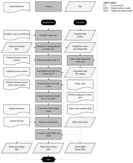
Figure 4.
SSegRef2Surf process.
3.3. 2D Simulation of the Flood Event February 2023
The verification of the classification and raster results of the SSegRef2Surf tool was carried out by comparing an existing and modified 2D model of the Aisch River, which covers the entire study area (Figure 5).
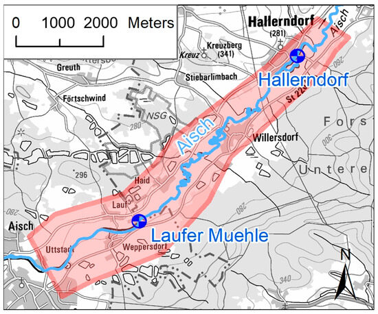
Figure 5.
Extent of the 2D model (red area) and location of stream gauging stations in the model area (blue circles) (map source: https://geodaten.bayern.de/opengeodata/, accessed on 27 January 2025).
The 2D model was provided by the Water Authority of Nuremberg (WWA-N). The model is used to calculate the ministerial designated floodplains along the Aisch River. The calibration of the model was carried out based on the flood event from October 1998 [54], which, with a discharge of 153 m3/s, corresponds approximately to a 20-year flood (a 20-year flood corresponds to a discharge of 155 m3/s, according to [55]). In the vicinity of the Laufer Muehle stream gauging station, the high water marks from in situ measurements during the flood event deviated by 6 and 19 cm from the simulation results. For the simulation of the February 2023 flood event (FE 02/2023), deviations of a similar magnitude were expected, as the event had a recurrence interval of less than an annual flood and discharge values of around 20 m3/s, which is significantly lower than the calibrated flood event. Despite the expected deviations, the existing 2D model was considered the best possible basis for a comparison with the UAV survey data, given the inclusion of current terrain information (DEM1 to DEM5 in the surrounding area) and available cross-section surveys.
The existing model was adapted to achieve a higher degree of comparability between in situ measurements and the 2D model for the Laufer Muehle study area. The 2D model provided by WWA-N was truncated to the relevant area around the Laufer Muehle stream gauging station, and an additional stream gauging station at Hallerndorf was included for controlling the hydraulic simulation results. We used Hydro-AS v.5.3.2 as simulation software. The inflow boundary condition was repositioned about 2.5 km upstream to minimize the influence of numerical disturbance effects, which can occur near inflow boundary conditions in 2D models, and to ensure a more realistic representation of the floodplains in the Laufer Muehle area. The in situ discharge values of the Laufer Muehle stream gauging station (steady state) were defined as boundary conditions of the model at the repositioned inflow boundary. The outlet boundary condition of the model (located approx. one kilometer downstream of the Hallerndorf stream gauging station) was defined with an energy line slope of 1‰.
The roughness parameter of the 2D model was adjusted in the Aisch River bed to better approximate the actual flow conditions during the flood event of February 2023. Figure 6 shows the comparison of the measured and simulated water levels at the Laufer Muehle stream gauging station.
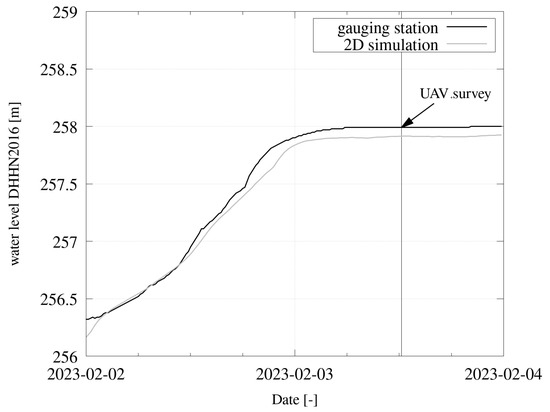
Figure 6.
Comparison between observed and simulated stage hydrograph at the Laufer Muehle stream gauging station. The arrow indicates the time of the UAV survey.
The distances between nodes in a 2D model are typically larger than the resolution of the available terrain models to ensure efficiency and a balanced relationship between the required spatial discretization and the simulation duration of each time step. However, in floodplain areas, it is common practice to overlay the simulated water surface elevation from the 2D model with the DEM to incorporate the higher-resolution information from the DEM.
A hydraulic DEM (water-DEM) represents the terrain, including the riverbed. The water-DEM is primarily used to depict water depths in the study area. In these investigations, the water-DEM was created based on a DEM1 and cross section measurements of the riverbed. This allows the riverbed to be taken into account when intersecting with the water surface elevations from the simulation results, leading to realistic water depth calculations. Thus, the simulation results can be transferred to a uniform grid corresponding to the highest possible spatial resolution of the terrain model. This result grid, with a 1 m resolution, was used to compare the SSegRef2Surf results with the 2D calculation results (Section 4.2).
3.4. Implementing SSegRef2Surf into the CDT
The change detection tool (CDT) developed by the authors of [50] enables near real-time analysis of changes in a study area by comparing multitemporal SfM data and visually validating the changes using orthophotos. The SSegRef2Surf postprocessing workflow presented in this study, which involves classifying an orthophoto and refining the classification results, was successfully integrated into the existing CDT. This implementation allows for near real-time analysis of changes before a flood event and the analysis of the flood extent during a flood event. The integration into the graphical user interface (GUI) facilitates the easy definition of calculation parameters and the initiation of the calculation. Figure 7 shows the input screen of SSegRef2Surf in conjunction with the CDT interface, as well as the parameter used in these studies and described in Section 3.2.

Figure 7.
GUI of the CDT showing the SSegRef2Surf parameter used in this study.
4. Results
4.1. t/Error Ratio for near Real-Time Flood Monitoring
Figure 8 illustrates the accuracy (horizontal) resulting from distance comparisons between ground control point (GCP) coordinates from GNSS-rover measurements using real-time kinematic (RTK) and those derived from UAV surveys.
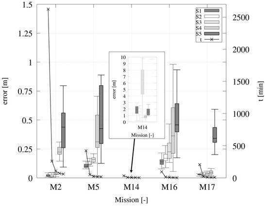
Figure 8.
Horizontal errors of orthophotos from SfM postprocessing with different settings (settings listed in Table 2) and their respective durations (t).
The results of M14 showed a minimum median error of 0.85 m and a maximum of 6.49 m, indicating very low accuracy. Although the postprocessing of this dataset allowed for the calculation of orthophotos in very short time intervals, the inaccuracies make these results unsuitable for high-precision analysis of flooded areas.
The error generally increases as accuracy parameters are reduced during the postprocessing of M2, M5, M16, and M17. The relationship between the increase in error and the reduction in accuracy parameters is approximately proportional between settings S1 and S3 for all missions. A disproportionate increase in error is observed (except for M17) between settings S3 and S4, which continues between S4 and S5.
The highest accuracy was achieved with M2 (S1–S3) and M17 (S1–S4), where the error remained ≤ 0.06 m. Across all settings, the error values for M17 were lower than those for M2. Since this study evaluated error determination only in the horizontal direction (xy-plane) and M17 (along with M16) operated at the highest flight altitude, it can be concluded that greater flight altitude allowed for better horizontal alignment of calculation results compared to missions surveyed at lower altitudes. Considering the vertical component (z-value), lower flight altitudes (and reduced ground sampling distance values) generally yield better results due to the higher ground sampling distance.
The most effective configuration in regard to processing time and error (best t/error ratio) was observed for orthophoto generation using M17 flight parameters combined with S3 postprocessing settings. In this case, the mean error was <0.03 m, with a postprocessing time of t = 11 min. This finding confirms the effectiveness of the M17 acquisition parameters, previously established in [27], which, when paired with the CDT developed in [50], achieved the best accuracy results.
M5 exhibited lower accuracy values despite longer postprocessing times. While M16 required less postprocessing time, its error significantly exceeded that of M17. Both M5 and M16 used the normal grid (NG) flight mode for surveying. The lower accuracy shows that the effectiveness of the double grid (DG) flight mode, as highlighted in [27], is also evident in the error values observed for orthophoto assessments.
The results show that the M17 acquisition parameters, combined with S3 postprocessing settings, are well suited for time-efficient and accurate documentation of flood events. Consequently, this combination was used to survey the flood event described in Section 2.
The implications of acquisition and postprocessing durations for near real-time flood analysis, as well as the impact of these findings on optimizing the CDT developed by the authors of [50], are discussed in Section 5.1.
4.2. Comparison of SSegRef2Surf and 2D Model Results
Figure 9 gives an overview of the results for the flood event of February 2023 from 2D analysis, the SVM classifier, and the results from SSegRef2Surf postprocessing, based on the orthophoto from M17 data. Figure 10 concretizes the differences by illustrating the extent of the water areas through three detailed views (Detail 1–3) to assess the functionality of the SSegRef2Surf tool and its comparability with the 2D calculation results.
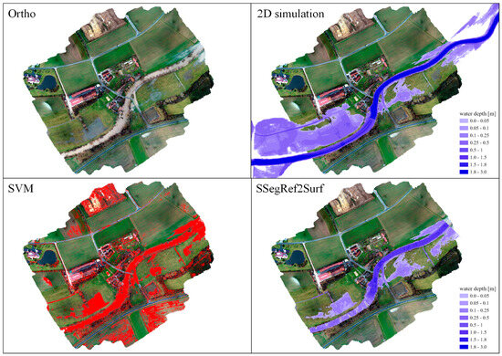
Figure 9.
Comparison of flooded areas from SVM classification, SSegRef2Surf postprocessing, and 2D numerical simulation of the flood event of February 2023 in the Laufer Muehle area.
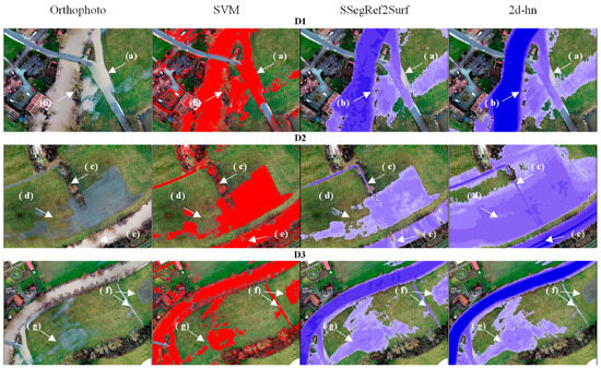
Figure 10.
Detail views (D1–D3) of significant areas (a–g) for comparison of flooded areas from SVM classification, SSegRef2Surf tool, and 2D numerical simulation of the flood event February 2023 in the Laufer Muehle area.
Position D1-(a) illustrates the impact of the accuracy of the DEM used in the SSegRef2Surf analysis. The SVM classification correctly identified a water area, but the DEM shows higher terrain elevations at this location than those observed during the survey. As a result of the higher terrain elevations, this area was removed during the extrapolation of the water surface elevation and the intersection with the DEM. This region is also absent in the 2D calculation results since the simulation results were clipped with the same DEM in the floodplain area.
The DEM used in these studies does not contain information about the riverbed. It is rather an extrapolation of the terrain elevation over the river area in the vicinity of the shoreline. Due to this extrapolation, water depths in the main flow section of the Aisch River (apart from the 2D model results) cannot be regarded as realistic. This is exemplified by D2-(e), where areas of missing water classification are visible in the SSegRef2Surf results. In general, better results in the main flow section can be achieved when implementing a DEM that also represents the riverbed (DEM-W).
D1-(b) and D2-(c) show water areas that were covered by vegetation but added to the results based on the DEM information. This shows that one of the key objectives of the SSegRef2Surf tool, namely, the refinement of areas that could not be detected by classification algorithms, was achieved.
D2-(d) shows that the flooded area, both in terms of extent and water depth, was significantly overestimated in the 2D results (almost across the entire detail area), while the SSegRef2Surf results provided a much more accurate match with the flooded area. The large flooded area in the 2D model was found to be due to insufficient consideration of the bank geometry in the model. While the water surface elevations intersected with the DEM do not suggest flooding of the left bank (as the banks rise several centimeters above the simulated water surface elevation), local overflow occurred at certain calculation nodes in the 2D model in the floodplain areas. Since both the in situ and simulated discharge at the Laufer Muehle stream gauging station remained nearly constant at about 22 m3/s prior to the UAV survey (Figure 5), the floodplain in the 2D model could be inundated during this period in areas with calculation nodes that were too low. The UAV image shown in Figure 11 confirms that there was no overflow of the banks in this area.
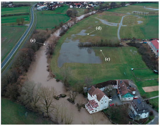
Figure 11.
Aerial image of the flooded area during the flood event of February 2023 in the upstream area of Laufer Muehle with localization of the detail areas (c–e) shown in Figure 10.
The 2D simulations did not include processes such as infiltration or groundwater flow. Since the water level of the Aisch River during the survey was almost at the same height as the floodplain, the water areas marked as (d) in the orthophoto and detected by the SVM may be attributed to infiltration water or groundwater. The results of the SSegRef2Surf tool can be valuable for validation and contribute to improving the understanding of these specific processes in 2D models.
SSegRef2Surf added a water surface in an area with no direct connection to the floodplain (D2-(d)) but with a lower elevation compared to the river’s water surface. This allowed for the inclusion of a water surface that existed during the flood event but likely resulted from prolonged rainfall or other inflows, such as from the adjacent ditch. In the case of very rapid flood events, this could lead to overestimations of the flooded areas. It is important to avoid these overestimations by monitoring and adjusting, for instance, by limiting the length of the cross sections within the SSegRef2Surf parameters.
Comparing the water area D3-(g) of the SVM and SSegRef2Surf results shows an overestimation of the water area extent, although the comparison between SSegRef2Surf and 2D model results shows a high degree of agreement. The overestimation results from the interpolation process using SSegRef2Surf and the DEM. The terrain elevation was considered too high in the interpolation process, resulting in false interpolation of the water surface height. D3-(f) shows additional areas that were identified using both the SVM and SSegRef2Surf but were not classified as flooded areas in the 2D simulations.
Figure 12 illustrates the difference in the flooded areas between the 2D simulations and the results from SSegRef2Surf. The white areas represent regions that are shown in both datasets, the red areas indicate additional flood areas in the 2D model results, and the blue areas represent additional flood areas in the SSegRef2Surf results. With regard to the matching (white) area (excluding differences within the riverbed), SSegRef2Surf optimized the flooded area by adding 11% (blue areas). The total area of the 2D simulations was reduced by 30% (red areas) by removing the overestimated areas.
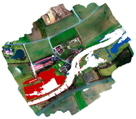
Figure 12.
Difference between SSegRef2Surf and 2D model results. Red: water area detected by 2D simulations but not by SSegRef2Surf. Blue: water area detected by SSegRef2Surf but not by 2D simulations. White: matching area.
5. Discussion
5.1. SSegRef2Surf Postprocessing to Improve Flood Area Raster Data
SSegRef2Surf integrates two-dimensional raster data with three-dimensional terrain information to correct misclassified water surfaces and supplement missing or occluded areas. This newly developed tool allows for the identification of water bodies that cannot be visually captured. It fills a data gap that has not been addressed by remote sensing or water classification algorithms, enabling the detection of flooding at relatively low water levels and in areas that are not visible (such as those covered by grass or shrubs), provided the overlaid DEM has sufficient accuracy.
This tool is designed for adaptability, allowing its calculation parameters to be adapted to specific study areas. It only requires the geometry of a water axis, a DEM, and a classified raster file as input files. In line with this flexible structure, SSegRef2Surf can be applied to a wide range of raster data, enabling the refinement of datasets from other classification processes.
In these investigations, a basic classification was performed using the SVM method with minimal preprocessing, which was refined by SSegRef2Surf. This workflow was validated for the Laufer Muehle study area through its strong alignment with 2D simulation results and visually identifiable flooded areas. Future studies should explore the applicability of this classification approach to other regions, particularly where the color features used for classification in this study differ significantly. For example, urban environments with dense infrastructure, such as roads and buildings, require different classification criteria than rural landscapes.
Water appearance on RGB images varies depending on factors such as depth and sediment concentration, with turbidity influencing color representation. In this study, both highly turbid water surfaces (brownish tones) and relatively clear water surfaces (bluish tones) were successfully identified as flooded areas (Figure 10, middle row, features e and d), demonstrating that, even with basic preprocessing, effective classification is achievable. Advanced methodologies, such as convolutional neural networks (CNNs), provide robust tools for extracting semantic information from RGB images with high accuracy. For example, refs. [17,33] achieved >95% accuracy in identifying inundated areas by training CNNs on 100 manually labeled images. This shows that pre-trained classifiers already exist that can accurately detect flooded areas in specific regions. However, even highly precise classification methods are limited by canopy and shadowed regions, which cannot be resolved solely through orthophoto classifying. The authors of [33] highlight that deep-learning-based approaches, such as CNNs, cannot directly derive water levels from 2D images. SSegRef2Surf addresses this gap by integrating terrain models to supplement these classifications with water level data.
Water look-alikes in satellite imagery, caused by surfaces like roads or radar shadows, often lead to erroneous water identifications in SAR satellite datasets [22]. These inaccuracies can be mitigated by combining such data with DEMs, as demonstrated in this study.
SSegRef2Surf enhances information quality and refines results by correlating low-resolution raster data with high-resolution DEMs. Classification outputs from satellite imagery, typically with resolutions exceeding 1 m per pixel, can be optimized through this approach. The increasing availability of freely accessible terrain data (e.g., DEM1) and the capability to use custom high-resolution models further expand SSegRef2Surf’s potential applications, making it a versatile and valuable tool for flood analysis and beyond.
This study demonstrates that, by combining aerial imagery with a digital elevation model (DEM), it is possible to identify water surfaces that are not visually detectable in the images (Figure 10, detail 2D-c). The level of detail in this identification depends on the accuracy and resolution (point density or grid spacing) of both the DEM and the SfM data, as well as the representative quality of the DEM itself. To ensure reliable results with SSegRef2Surf, the DEM must accurately represent the bare-earth surface, free of vegetation. If the DEM incorrectly includes dense vegetation, such as grass or shrubs, as part of the terrain surface, this can lead to an overestimation of elevation when combined with the identified water surfaces. The overestimation of terrain elevation leads to inaccurate results when compared to the water surface elevation, causing areas to be incorrectly identified as dry land instead of flooded areas.
A high-quality DEM is essential for reliably identifying water surfaces in areas with dense vegetation coverage. This includes both the accuracy of the terrain representation and the resolution of the model. When these two parameters are sufficiently considered, it is possible to identify flood areas, even in regions with low water depths and dense vegetation coverage.
5.2. Near Real-Time Flood Mapping Possibilities
Flooded areas can be visually assessed in a very short time based on orthophotos and using the method presented in this study. The use of UAVs offers flexibility in defining the study area and thus enhances applicability during a flood event. To evaluate the spatio-temporal analysis capabilities of the used methods and workflows, it is essential to differentiate between the following aspects:
- Frequency and duration of surveys (mapping interval);
- Postprocessing duration to generate a visual representation (orthophoto) using SfM (SfM orthophoto);
- Postprocessing duration for classification and georeferencing of the flood area.
The total time required for these three steps, assuming a UAV setup time (including return flight, data retrieval, data transfer, and changing battery) of five minutes, is shown in Figure 13.
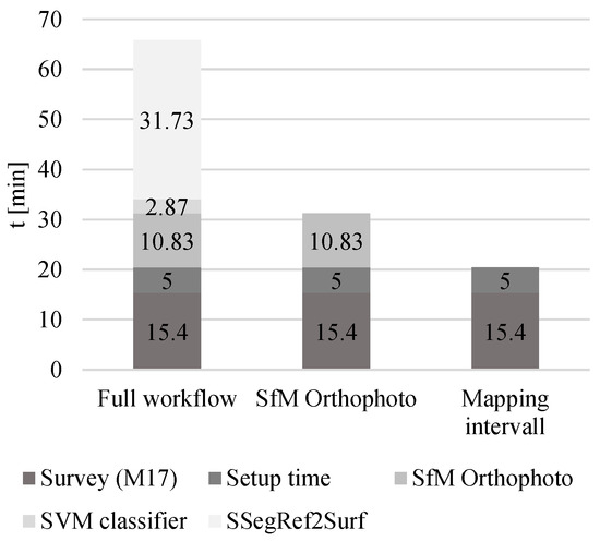
Figure 13.
Durations of the near real-time flood mapping processes.
Our results show the following, if the developed workflow, postprocessing optimizations, and the SSegRef2Surf tool are used:
- An approximately 0.4 km2 area can be surveyed at high resolution every 21 min;
- An orthophoto can be produced 11 min later (total duration ≈ 32 min);
- The orthophoto can be classified and georeferenced to identify the flooded area in an additional 34 min (total duration ≈ 66 min).
This high survey frequency enables detailed analysis of the development of a flood event. Using SeegRef2Surf, a flood event can be assessed, and critical visual data can be provided to authorities and emergency services in under half an hour. Additionally, the high-frequency analysis of the flooded area ensures detailed traceability of the temporal development of the flood extent.
In this study, a multicopter UAV was used to survey the Laufer Muehle area. Fixed-wing UAV systems are able to survey multiple square kilometers per hour [56]. Combining fixed-wing UAV systems with high-resolution camera setups could extend the applicability of the methods presented in this study by considering GSD specifications. Future studies should investigate the transferability of these results and the applicability of the SSegRef2Surf tool to such systems.
Fixed ground-based sensor systems, such as those used in [57] (e.g., RGB camera modules), represent another method with minimal time requirements for near real-time monitoring of water surfaces. Using these systems enables high-accuracy remote sensing with high temporal resolution and leads to insights on a local or regional scale. However, as previously described in Section 1.2, these sensors are “[…] limited [in] spatial coverage” [58].
Compared to UAV SfM surveys, satellite systems can detect water surfaces and monitor flood events by capturing entire river basins in a single overpass and identifying flooded areas using various survey and postprocessing methods. SAR satellite systems can operate during cloudy conditions, which are common during flood events, as well as at night [20,21,59,60]. However, their revisit time is typically several days [43], resulting in lower temporal resolution compared to UAV surveys. Optical satellites, on the other hand, are limited by their inability to penetrate clouds. Their observations can only occur during daytime and under favorable weather conditions [43], which further extends their acquisition intervals. UAVs offer an advantage in this regard, as they can operate below cloud cover, enabling surveys during conditions that are inaccessible to optical satellite systems [15]. Due to their significant distance from the Earth’s surface, satellite systems generally offer lower spatial resolution (usually ranging from 30 m to 1 m [49]), which limits their ability to generate high-resolution flood area maps.
The results of this study, combining optimized SfM postprocessing for orthophoto creation, SVM-based classification, and the newly developed SSegRef2Surf postprocessing tool, demonstrate that UAVs equipped with RGB camera systems are a suitable method for capturing flood events with high spatio-temporal resolution.
5.3. High Accuracy Flood Maps
The workflow presented in this study enables highly accurate surveying of flood events, making it possible to generate a georeferenced flood area with sub-decimeter precision in approximately an hour for an area of approximately 0.4 km2. Flood areas obscured by canopy, shadows, bridges, or buildings, which pose challenges for identification through remote sensing and deep learning [17], can be supplemented using the SSegRef2Surf tool by combining topographic and visual information.
The analysis conducted in this study was based on orthophotos with a 5 cm resolution (downscaled) and a positional error of less than 3 cm. These data allow for the generation of highly detailed water surface maps that surpass the resolution of typical 2D model results (which often have resolutions of several meters). Due to limitations in current ArcGIS versions (v. 3.3.1 used in this study), SSegRef2Surf results can only be exported as raster files with a 1 m resolution, reducing the resolution of the output. However, this resolution is sufficient for comparison with 2D model results and for near real-time assessment of flooded areas.
The significance and benefit of this accuracy are illustrated by the flooded area presented in Figure 10, detail D2-(d). Due to the insufficient representation of the riverbank in the 2D model, a transitional flow into the floodplain was simulated. This resulted in an extensive area being incorrectly classified as flooded, with the water depth several decimeters too high compared to the actual flooded area. Particularly in the context of unsteady simulations, where calculations are continued until the difference in water level becomes negligible, even small inaccuracies in the model representation can lead to the flooding of entire floodplains. The high accuracy of the SSegRef2Surf tool enables the identification of erroneous flow paths in the numerical simulations, thus preventing misleading representations of flooded areas, such as those in flood risk and flood hazard maps.
5.4. Improving 2D Model Results
Data from stream gauging stations in conjunction with flood marks of past flood events are essential and typically used to calibrate and validate 2D models [10]. However, stream gauging stations are usually located several kilometers apart along a river, resulting in relatively low data density, considering changes in discharge along the river (e.g., through tributaries). Stream gauging stations can fail during extreme flood events, as demonstrated during the event on the Ahr River in July 2021, when five out of eight stations stopped functioning [13]. As the authors of [15] (p. 1) point out, stream gauging stations “[…] provide invaluable point-scale water level/discharge estimates at selected locations, [but] the lack of real-time data on inundated areas adjacent to river channels is a major limitation to accurate assessment of existing flood conditions”.
Generally, flood risk and hazard maps are derived from the results of 2D simulations for specific flood events (e.g., 100-year-flood). It is crucial to conduct their calibration using the highest possible data density to ensure the high quality of these maps. The use of remote sensing data allows not only the determination of water levels at many different locations but also the generation of high spatio-temporal resolution datasets that provide significantly denser information. Using SSegRef2Surf, we managed to evaluate existing findings in the Laufer Muehle area. For example, according to [55], the stream gauging station becomes surrounded by water at a discharge of about 28 m3/s (value obtained from a 2D model). However, the results of the UAV survey on 02/2023 and the in situ measurement of the stream gauging station revealed that the station was already surrounded at a discharge of 21.5 m3/s (about 6.5 m3/s earlier than previously assumed). Thus, the SSegRef2Surf analysis demonstrated that the stream gauging station becomes surrounded significantly earlier than initially estimated (Figure 14).
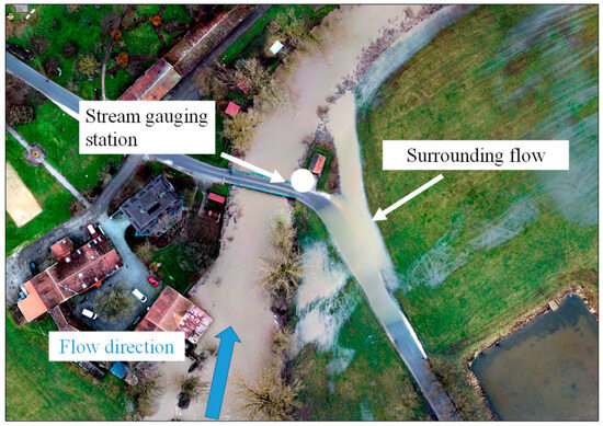
Figure 14.
Bypassing flow at the Laufer Muehle stream gauging station during the flood event of February 2023 (Q = 21.5 m3/s).
Whether the onset of the surrounding flow occurred upstream or downstream of the gauging station cannot be determined based on the results of one single survey. This shows that, as one of the conclusions of [14] suggests, it is necessary to have a comprehensive set of data to improve the results of hydraulic calculations. Remote sensing, especially in combination with UAV, SfM, and SSegRef2Surf, offers significant potential to provide near real-time information on the development of flooded areas, validate models, and ultimately enhance flood protection concepts. With a mapping interval of approximately 21 min, the method requires only slightly more time than the data acquisition of the stream gauging station (15 min at Laufer Muehle) but provides significantly more extensive data.
5.5. Correlation of DEM and Semantic Segmentation to Determine Water Depth
One advantage of raster-based analysis is its ability to facilitate the straightforward comparison of datasets in a two-dimensional format. In the case of a flood event, this comparison allows for determining the temporal development and extent of the flooded area. However, the two-dimensional simplification means that elevation data cannot be directly considered. Statements about three-dimensional quantities (water depth) can only be generated by overlaying with other data sources. With SSegRef2Surf, water depths can be determined by overlaying with terrain data (DEM), which can be used for validating 2D models. Figure 15 shows the difference between the water depths from SSegRef2Surf and the 2D model.
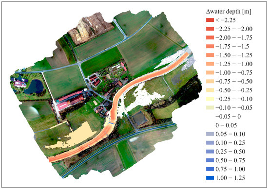
Figure 15.
Water depth difference in overlapping areas between SSegRef2Surf results and 2D simulation. A positive value indicates a higher water depth in the SSegRef2Surf results and vice versa.
The white-colored areas in Figure 15 indicate regions with high agreement between SSegRef2Surf and 2D simulation results (difference ± 5 cm). These areas are located near the gauging station, aligning with the findings from Section 4.2. The large differences in the main channel result from the fact that the DEM used in the SSegRef2Surf calculation is derived from airborne laser scanning data and thus does not include bathymetric information (riverbed data), since laser signals are reflected on the water surface. As a result, the riverbed elevation was assumed to be higher than it actually was, leading to an underestimation of the water depth.
Deviations between 2D simulation and SSegRef2Surf results are evident in the area upstream of the stream gauging station, where water depths in the 2D simulations were significantly deeper than in the SSegRef2Surf results. This is due to the overestimation of the water level in the 2D model, as discussed in Section 4.2.
The large differences in the main channel result from the fact that the DEM used in the SSegRef2Surf calculation did not include bathymetric information (riverbed terrain data). As a result, the riverbed elevation was assumed to be higher than it actually was, leading to an underestimation of the water depth.
5.6. Optimizing CDT Efficiency
While enabling near real-time mapping of flood events was the main focus of these studies, the optimization of the change detection process in the CDT was also a key focus. The findings in [50] showed that, by optimizing individual subprocesses, the calculation of an orthophoto for visualizing the detected changes in the study area constituted the largest portion of the total processing time. The optimization of the SfM process for generating an orthophoto, as presented in this study, was applied to the CDT analysis, reducing the total processing time of the CDT from approx. 24 min to approx. 16 min (for surveying an area of approx. 0.4 km2).
6. Conclusions and Future Prospects
The newly developed SSegRef2Surf tool enables the identification of water bodies even in areas undetectable by conventional remote sensing systems. Even with low data density (a single orthophoto), a roughly trained classifier (support vector machine), widely used UAV systems, and openly available geospatial datasets (DEM, water axis), postprocessing with SSegRef2Surf achieves a strong agreement with visually identifiable flooded areas (from orthophotos), which makes it applicable for a wide range of flood mapping systems and postprocessing algorithms.
Studies show that the combination of optimized postprocessing parameters, highly efficient survey parameters, fully automated workflows, and the application of the SSegRef2Surf tool enables the following:
- High-resolution surveying of flood areas of approximately 0.4 km2 every 21 min (with DJI Phantom 4 RTK);
- Generation of an orthophoto 11 min later (total duration approximately 32 min);
- Identification of the classified and georeferenced flooded area an additional 34 min later (total duration approximately 66 min).
Regions obscured by vegetation or shadowed by infrastructure during the UAV survey were supplemented with an intersection with terrain geometry (DEM). This process enabled the combination of classification results with geometric attributes (e.g., water depth, and water level), allowing for filtering and refinement using SSegRef2Surf.
The comparison between 2D results and SSegRef2Surf showed that 30% of the flooded areas identified in the 2D numerical results were incorrect. A total of 11% of the visually recognizable flooded area was not represented by the 2D model. This demonstrates the significant optimization potential provided by the SSegRef2Surf analysis.
The SSegRef2Surf postprocessing method should be extended to additional measurement systems, such as fixed-wing UAVs, to enable the surveying of larger areas for flood monitoring in future research. Ref. [15] describes a fixed-wing UAV system capable of mapping approximately 324 km2 in 2.5 h. This shows that using fixed-wing UAVs enables high-frequency surveying of entire river systems during flood events. The high-density, near-real-time data of flood events are crucial for decision-making during these events and support the evaluation and optimization of numerical simulations to improve their accuracy. However, the ground sampling distance (GSD) of about 16 cm using the system in [15] was lower than the GSD of this study (3.01 cm). By considering the results and GSD values from this study, our findings can be transferred to other UAV and camera systems with comparable accuracy. In cases of lower accuracy, postprocessing parameters should be adjusted accordingly.
A limiting factor in UAV-based data acquisition is compliance with legal regulations. While smaller river sections in the European Union can be surveyed within the Open Category under visual line of sight conditions, mapping entire river systems using a fixed-wing UAV falls under the Specific Category [61]. Operations in this category require a risk assessment, which must be conducted specifically for the process of surveying a river system during a flood event. In this context, large-scale events necessitate coordination with additional emergency response entities, such as disaster management agencies and helicopters operating in the area.
Adverse weather conditions can limit the use of UAVs during flood events. Strong wind gusts and rainfall, which frequently occur in such situations, pose a risk of damaging the system during operation. The use of resilient UAV systems equipped with fail-safe mechanisms, such as parachute recovery systems, is particularly crucial for operations in the Specific Category, especially in beyond visual line of sight (BVLOS) missions.
If UAV deployment is not feasible due to weather conditions or regulatory restrictions, manned aircraft can be considered as an alternative for flood event surveying. Compared to UAVs, manned aircraft are generally less susceptible to rain and wind, can operate at higher altitudes and speeds, and are capable of covering large areas efficiently. For instance, [62] developed a system to transform an ultralight aircraft (AutoGyro MTOsport gyrocopter) into a “… a full-fledged aerial remote sensing platform…” [62] (p. 1). The high availability of such gyrocopters (approximately 500 in Germany [62]) allows for flexible deployment. If legal or weather conditions prevent UAV-based data acquisition, flood event mapping over large areas can still be achieved by combining other unmanned aerial systems with near real-time postprocessing using SSegRef2Surf.
Since SSegRef2Surf was developed to process a wide range of raster data, users can apply this tool for the post-processing of satellite data (e.g., Sentinel-1 and Sentinel-2). This data source provides extensive global datasets of past flood events. The interpolation properties of SSegRef2Surf help densify the relatively sparse raster data of these flood events. Densifying these data enables more precise statements about the extent of flood areas, which enhances the optimization and calibration of 2D models.
Author Contributions
Conceptualization, M.K., L.F. and F.M.; methodology, M.K., L.F. and F.M.; software, M.K. and L.F.; validation, M.K. and L.F.; formal analysis, M.K.; investigation, M.K. and L.F.; resources, D.C.; data curation, M.K.; writing—original draft preparation, M.K.; writing—review and editing, M.K., F.M. and D.C.; visualization, M.K.; supervision, M.K.; project administration, M.K.; funding acquisition, M.K., F.M. and D.C. All authors have read and agreed to the published version of the manuscript.
Funding
The preceding investigations of this work were supported by the STAEDTLER Foundation (travel, material/equipment, and personnel costs). The investigations presented here were funded by Technische Hochschule Nürnberg Georg Simon Ohm as part of the “Initial Research Initiative” (German: Initiative der Vorlaufforschung, Funding number 664101004), which exclusively covered personnel costs.
Data Availability Statement
The code for the SSegRef2Surf tool presented in this article is not currently available for general use, as it is limited to the developer’s specific computing environment and requires highly specific software versions. We are actively working to enhance the code’s usability and make it publicly accessible. Requests for access to the current version of the code can be directed to the corresponding author (Michael Kögel).
Conflicts of Interest
The authors declare no conflicts of interest.
Abbreviations
The following abbreviations are used in this manuscript:
| 2D | Two-dimensional |
| 3D | Three-dimensional |
| AI | Artificial intelligence |
| BDD | Build Depth Maps Downscale |
| CD | Change detection |
| CDT | Change detection tool |
| CNN | Convolutional neural network |
| DEM | Digital elevation model |
| DEM1 | Digital terrain model with a 1 m grid |
| DEM5 | Digital terrain model with a 5 m grid |
| DG | Double grid |
| DSM | Digital surface models |
| EG-HWRM-RL | Hochwasserrisikomanagement-Richtlinie der Europäischen Gemeinschaft (engl. European Flood Risk Management Directive) |
| ESA | European Space Agency |
| EU-FRMD | European Flood Risk Management Directive |
| FE | Flood event |
| GCP | Ground control points |
| GNSS | Global Navigation Satellite System |
| GSD | Ground sampling distance |
| GUI | Graphical user interface |
| HPC | High-performance cluster |
| LAWA | Federal/State Working Group on Water. German: Bund/Länder-Arbeitsgemeinschaft Wasser |
| LiDAR | Light Detection and Ranging |
| MPD | Match Photos Downscale |
| NASA | National Aeronautics and Space Administration |
| NG | Normal grid |
| RGB | Red, green, and blue |
| RTK | Real-time kinematic |
| SAPOS | Satellitenpositionierungsdienst der deutschen Landesvermessung (engl. satellite positioning service of the German national survey) |
| SAR | Synthetic Aperture Radar |
| SfM | Structure from Motion |
| SSegRef2Surf | Semantic Segmentation Refinement to create 2D Water Surfaces |
| SVM | Support vector machine |
| UAV | Unmanned aerial vehicle |
| USGS | United States Geological Survey |
| WWA-N | Water Authority of Nuremberg |
References
- Blöschl, G.; Hall, J.; Viglione, A.; Perdigão, R.A.P.; Parajka, J.; Merz, B.; Lun, D.; Arheimer, B.; Aronica, G.T.; Bilibashi, A.; et al. Changing climate both increases and decreases European river floods. Nature 2019, 573, 108–111. [Google Scholar] [CrossRef] [PubMed]
- Umweltbundesamt. 2019 Monitoring Report on the German Strategy for Adaptation to Climate Change: Report by the Interministerial Working Group on Adaptation to Climate Change; Umweltbundesamt: Dessau-Roßlau, Germany, 2019. [Google Scholar]
- Patt, H.; Gonsowski, P. Wasserbau, 7th ed.; Springer: Berlin/Heidelberg, Germany, 2011; ISBN 978-3-642-11962-0. [Google Scholar]
- LAWA. Leitlinien für Einen Zukunftsweisenden Hochwasserschutz—Hochwasser—Ursachen und Konsequenzen; LAWA: Stuttgart, Germany, 1995. [Google Scholar]
- EG. Richtlinie 2007/60/EG des Europäischen Parlaments und des Rates vom 23. Oktober 2007 über die Bewertung und das Management von Hochwasserrisiken: (ABl. L 288 vom 06.11.2007, S. 27); EG: Hamburg, Germany, 2007. [Google Scholar]
- LAWA. Instrumente und Handlungsempfehlungen zur Umsetzung der Leitlinien für Einen Zukunftsweisenden Hochwasserschutz; LAWA: Düsseldorf, Germany, 2004. [Google Scholar]
- LAWA. Empfehlungen—Oberirdische Gewässer: Gewässerstrukturgütekartierung in der Bundesrepublik Deutschland—Verfahren für Kleine und Mittelgroße Fließgewässer; LAWA: Schwerin, Germany, 1999. [Google Scholar]
- LAWA. Handlungsempfehlung zur Erstellung von Hochwasser-Aktionsplänen; LAWA: Schwerin, Germany, 2000. [Google Scholar]
- LAWA. Empfehlungen zur Aufstellung von Hochwasserrisikomanagementplänen; LAWA: Dresden, Germany, 2019. [Google Scholar]
- LAWA. Empfehlungen der Bund/Länder Arbeitsgemeinschaft Wasser zur Aufstellung von Hochwassergefahrenkarten und Hochwasserrisikokarten; LAWA: Dresden, Germany, 2010. [Google Scholar]
- LAWA. Empfehlungen der Bund/Länder Arbeitsgemeinschaft Wasser zur Aufstellung von Hochwassergefahrenkarten und Hochwasserrisikokarten; LAWA: Weimar, Germany, 2018. [Google Scholar]
- Muhadi, N.A.; Abdullah, A.F.; Bejo, S.K.; Mahadi, M.R.; Mijic, A. The Use of LiDAR-Derived DEM in Flood Applications: A Review. Remote Sens. 2020, 12, 2308. [Google Scholar] [CrossRef]
- DKKV. Governance und Kommunikation im Krisenfall des Hochwasserereignisses im Juli 2021; DKKV: Bonn, Germany, 2024. [Google Scholar]
- Müller, U. Hochwasserrisikomanagement; Vieweg+Teubner: Wiesbaden, Germany, 2010; ISBN 978-3-8348-1247-6. [Google Scholar]
- Dyer, J.L.; Moorhead, R.J.; Hathcock, L. Identification and Analysis of Microscale Hydrologic Flood Impacts Using Unmanned Aerial Systems. Remote Sens. 2020, 12, 1549. [Google Scholar] [CrossRef]
- Langhammer, J.; Vacková, T. Detection and Mapping of the Geomorphic Effects of Flooding Using UAV Photogrammetry. Pure Appl. Geophys. 2018, 175, 3223–3245. [Google Scholar] [CrossRef]
- Gebrehiwot, A.; Hashemi-Beni, L.; Thompson, G.; Kordjamshidi, P.; Langan, T.E. Deep Convolutional Neural Network for Flood Extent Mapping Using Unmanned Aerial Vehicles Data. Sensors 2019, 19, 1486. [Google Scholar] [CrossRef]
- Merz, B. Hochwasserrisiken: Grenzen und Möglichkeiten der Risikoabschätzung; Schweizerbart: Stuttgart, Germany, 2006; ISBN 3-510-65220-7. [Google Scholar]
- Patt, H.; Jüpner, R. (Eds.) Hochwasser-Handbuch: Auswirkungen und Schutz, 3rd ed.; Springer Vieweg: Wiesbaden, Germany, 2020; ISBN 978-3-658-26742-1. [Google Scholar]
- Refice, A.; Capolongo, D.; Chini, M.; D’Addabbo, A. Improving Flood Detection and Monitoring through Remote Sensing. Water 2022, 14, 364. [Google Scholar] [CrossRef]
- Katiyar, V.; Tamkuan, N.; Nagai, M. Near-Real-Time Flood Mapping Using Off-the-Shelf Models with SAR Imagery and Deep Learning. Remote Sens. 2021, 13, 2334. [Google Scholar] [CrossRef]
- Colacicco, R.; Refice, A.; Nutricato, R.; Bovenga, F.; Caporusso, G.; D’Addabbo, A.; La Salandra, M.; Lovergine, F.P.; Nitti, D.O.; Capolongo, D. High-Resolution Flood Monitoring Based on Advanced Statistical Modeling of Sentinel-1 Multi-Temporal Stacks. Remote Sens. 2024, 16, 294. [Google Scholar] [CrossRef]
- Farmakis, I.; DiFrancesco, P.-M.; Hutchinson, D.J.; Vlachopoulos, N. Rockfall detection using LiDAR and deep learning. Eng. Geol. 2022, 309, 106836. [Google Scholar] [CrossRef]
- Blanch, X.; Abellan, A.; Guinau, M. Point Cloud Stacking: A Workflow to Enhance 3D Monitoring Capabilities Using Time-Lapse Cameras. Remote Sens. 2020, 12, 1240. [Google Scholar] [CrossRef]
- Blanch, X.; Eltner, A.; Guinau, M.; Abellan, A. Multi-Epoch and Multi-Imagery (MEMI) Photogrammetric Workflow for Enhanced Change Detection Using Time-Lapse Cameras. Remote Sens. 2021, 13, 1460. [Google Scholar] [CrossRef]
- Blanch, X.; Guinau, M.; Eltner, A.; Abellan, A. Fixed photogrammetric systems for natural hazard monitoring with high spatio-temporal resolution. Nat. Hazards Earth Syst. Sci. 2023, 23, 3285–3303. [Google Scholar] [CrossRef]
- Kögel, M.; Carstensen, D. Using structure from motion for analyzing change detection and flood events in the context of flood preparedness: A case study for the Laufer Muehle area at the Aisch river in Germany for conducting near real-time analyses. Appl. Geomat. 2024, 16, 409–427. [Google Scholar] [CrossRef]
- Langhammer, J.; Bernsteinová, J.; Miřijovský, J. Building a High-Precision 2D Hydrodynamic Flood Model Using UAV Photogrammetry and Sensor Network Monitoring. Water 2017, 9, 861. [Google Scholar] [CrossRef]
- Li, W.; Li, Y.; Gong, J.; Feng, Q.; Zhou, J.; Sun, J.; Shi, C.; Hu, W. Urban Water Extraction with UAV High-Resolution Remote Sensing Data Based on an Improved U-Net Model. Remote Sens. 2021, 13, 3165. [Google Scholar] [CrossRef]
- Eltner, A.; Hoffmeister, D.; Kaiser, A.; Karrasch, P.; Klingbeil, L.; Stöcker, C.; Rovere, A. (Eds.) UAVs for the Environmental Sciences: Methods and Applications; wbg Academic: Darmstadt, Germany, 2022; ISBN 978-3-534-40588-6. [Google Scholar]
- Vélez-Nicolás, M.; García-López, S.; Barbero, L.; Ruiz-Ortiz, V.; Sánchez-Bellón, Á. Applications of Unmanned Aerial Systems (UASs) in Hydrology: A Review. Remote Sens. 2021, 13, 1359. [Google Scholar] [CrossRef]
- Kögel, M.; Pflitsch, A.; Northup, D.E.; Carstensen, D.; Medley, J.J.; Mansheim, T.; Killing, T.; Buschbacher, M.; Angerer, H.; Falkner, J.; et al. Combination of close-range and aerial photogrammetry with terrestrial laser scanning to answer microbiological and climatological questions in connection with lava caves. Appl. Geomat. 2022, 14, 679–694. [Google Scholar] [CrossRef]
- Gebrehiwot, A.; Hashemi-Beni, L. A Method to Generate Flood Maps in 3d Using dem and Deep Learning. Int. Arch. Photogramm. Remote Sens. Spat. Inf. Sci. 2020, XLIV-M-2-2020, 25–28. [Google Scholar] [CrossRef]
- Duguay, J.; Lindenschmidt, K.-E.; Trudel, M.; Pruneau, A. Aerial photogrammetry to characterise and numerically model an ice jam in Southern Quebec. Hydrol. Res. 2023, 54, 1329–1343. [Google Scholar] [CrossRef]
- Hashemi-Beni, L.; Jones, J.; Thompson, G.; Johnson, C.; Gebrehiwot, A. Challenges and Opportunities for UAV-Based Digital Elevation Model Generation for Flood-Risk Management: A Case of Princeville, North Carolina. Sensors 2018, 18, 3843. [Google Scholar] [CrossRef]
- Dinkel, A.; Hoegner, L.; Emmert, A.; Raffl, L.; Stilla, U. Change detection in photogrammetric point clouds for monitoring of alpine, gravitational mass movements. ISPRS Ann. Photogramm. Remote Sens. Spat. Inf. Sci. 2020, V-2-2020, 687–693. [Google Scholar] [CrossRef]
- Andresen, C.G.; Schultz-Fellenz, E.S. Change Detection Applications in the Earth Sciences Using UAS-Based Sensing: A Review and Future Opportunities. Drones 2023, 7, 258. [Google Scholar] [CrossRef]
- Mancini, F.; Salvini, R. Applications of Photogrammetry for Environmental Research. ISPRS Int. J. Geo-Inf. 2019, 8, 542. [Google Scholar] [CrossRef]
- Okyay, U.; Telling, J.; Glennie, C.L.; Dietrich, W.E. Airborne lidar change detection: An overview of Earth sciences applications. Earth-Sci. Rev. 2019, 198, 102929. [Google Scholar] [CrossRef]
- Salas, E.A.L. Waveform LiDAR concepts and applications for potential vegetation phenology monitoring and modeling: A comprehensive review. Geo-Spat. Inf. Sci. 2021, 24, 179–200. [Google Scholar] [CrossRef]
- Shen, G.; Fu, W.; Guo, H.; Liao, J. Water Body Mapping Using Long Time Series Sentinel-1 SAR Data in Poyang Lake. Water 2022, 14, 1902. [Google Scholar] [CrossRef]
- Kögel, M.; Das, A.; Marszelewski, W.; Carstensen, D.; Lindenschmidt, K.-E. Machbarkeitsstudie zur Vorhersage von Eisstau auf der Oder. Wasserwirtsch 2017, 107, 20–28. [Google Scholar] [CrossRef]
- Tarpanelli, A.; Mondini, A.C.; Camici, S. Effectiveness of Sentinel-1 and Sentinel-2 for flood detection assessment in Europe. Nat. Hazards Earth Syst. Sci. 2022, 22, 2473–2489. [Google Scholar] [CrossRef]
- Möldner, F.; Hentschel, B.; Carstensen, D. Ice-Jam Investigations along the Oder River Based on Satellite and UAV Data. Water 2024, 16, 1323. [Google Scholar] [CrossRef]
- Schlaffer, S.; Chini, M.; Dorigo, W.; Plank, S. Monitoring surface water dynamics in the Prairie Pothole Region of North Dakota using dual-polarised Sentinel-1 synthetic aperture radar (SAR) time series. Hydrol. Earth Syst. Sci. 2022, 26, 841–860. [Google Scholar] [CrossRef]
- Bentivoglio, R.; Isufi, E.; Jonkman, S.N.; Taormina, R. Deep Learning Methods for Flood Mapping: A Review of Existing Applications and Future Research Directions. Hydrol. Earth Syst. Sci. 2021, 26, 4345–4378. [Google Scholar] [CrossRef]
- Hernández, D.; Cecilia, J.M.; Cano, J.-C.; Calafate, C.T. Flood Detection Using Real-Time Image Segmentation from Unmanned Aerial Vehicles on Edge-Computing Platform. Remote Sens. 2022, 14, 223. [Google Scholar] [CrossRef]
- Karamuz, E.; Romanowicz, R.J.; Doroszkiewicz, J. The use of unmanned aerial vehicles in flood hazard assessment. J. Flood Risk Manag. 2020, 13, e12622. [Google Scholar] [CrossRef]
- Sadiq, R.; Imran, M.; Ofli, F. Remote Sensing for Flood Mapping and Monitoring. In International Handbook of Disaster Research; Singh, A., Ed.; Springer Nature: Singapore, 2022; pp. 1–19. ISBN 978-981-16-8800-3. [Google Scholar]
- Kögel, M.; Carstensen, D. Near real-time change detection tool for photogrammetric flood preparedness. Environ. Monit. Assess. 2025, 197, 129. [Google Scholar] [CrossRef]
- Bayerisches Landesamt für Umwelt. Gewässerkundlicher Dienst Bayern: Messdaten Laufer Mühle—Messstellen-Nr.: 24263000. 2024. Available online: https://www.gkd.bayern.de/de/fluesse/abfluss/bayern/laufermuehle-24263000 (accessed on 11 March 2025).
- SAPOS. Produktdefinition SAPOS. Available online: https://www.sapos.de/files/SAPOS-Produktdefinition_2017.pdf (accessed on 11 March 2025).
- Agisoft LLC. Metashape Python Reference: Release, version 1.8.4; Agisoft LLC: St. Petersburg, Russia, 2022. [Google Scholar]
- RMD-Consult GmbH. 2-D-WSP-Berechnungen Aisch: Abschlussbericht; RMD-Consult GmbH: München, Germany, 2010. [Google Scholar]
- Bayerisches Landesamt für Umwelt. Hochwassernachrichtendienst Bayern: Abfluss Laufermühle/Aisch. Available online: https://www.hnd.bayern.de/pegel/regnitz/laufermuehle-24263000/stammdaten? (accessed on 22 January 2025).
- Feng, Q.; Liu, J.; Gong, J. Urban Flood Mapping Based on Unmanned Aerial Vehicle Remote Sensing and Random Forest Classifier—A Case of Yuyao, China. Water 2015, 7, 1437–1455. [Google Scholar] [CrossRef]
- Eltner, A.; Bressan, P.O.; Akiyama, T.; Gonçalves, W.N.; Marcato Junior, J. Using Deep Learning for Automatic Water Stage Measurements. Water Resour. Res. 2021, 57, e2020WR027608. [Google Scholar] [CrossRef]
- Wienhold, K.J.; Li, D.; Li, W.; Fang, Z.N. Flood Inundation and Depth Mapping Using Unmanned Aerial Vehicles Combined with High-Resolution Multispectral Imagery. Hydrology 2023, 10, 158. [Google Scholar] [CrossRef]
- Bioresita, F.; Puissant, A.; Stumpf, A.; Malet, J.-P. A Method for Automatic and Rapid Mapping of Water Surfaces from Sentinel-1 Imagery. Remote Sens. 2018, 10, 217. [Google Scholar] [CrossRef]
- Kuntla, S.K. An era of Sentinels in flood management: Potential of Sentinel-1, -2, and -3 satellites for effective flood management. Open Geosci. 2021, 13, 1616–1642. [Google Scholar] [CrossRef]
- European Union: Commission Implementing Regulation (EU) 2019/947 of 24 May 2019 on the Rules and Procedures for the Operation of Unmanned Aircraft. Available online: https://eur-lex.europa.eu/legal-content/EN/TXT/PDF/?uri=OJ:L:2019:152:FULL (accessed on 11 March 2025).
- Jenal, A.; Kneer, C.; Weber, I.; Asgari, M.; Knieps, M.; Bongartz, J. An Adaptive Sensor Framework for Gyrocopter-Based Optical Remote Sensing: Introduction and Applications. PFG—J. Photogramm. Remote Sens. Geoinf. Sci. 2022, 90, 93–101. [Google Scholar] [CrossRef]
Disclaimer/Publisher’s Note: The statements, opinions and data contained in all publications are solely those of the individual author(s) and contributor(s) and not of MDPI and/or the editor(s). MDPI and/or the editor(s) disclaim responsibility for any injury to people or property resulting from any ideas, methods, instructions or products referred to in the content. |
© 2025 by the authors. Licensee MDPI, Basel, Switzerland. This article is an open access article distributed under the terms and conditions of the Creative Commons Attribution (CC BY) license (https://creativecommons.org/licenses/by/4.0/).