A Robust InSAR-DEM Block Adjustment Method Based on Affine and Polynomial Models for Geometric Distortion

Abstract

DEMs derived from Interferometric Synthetic Aperture Radar (InSAR) imagery are frequently influenced by multiple factors, resulting in systematic horizontal and elevation inaccuracies that affect their applicability in large-scale scenarios. To mitigate this problem, this study employs affine models and polynomial function models to refine the relative planar precision and elevation accuracy of the DEM. To acquire high-quality control data for the adjustment model, this study introduces a DEM feature matching method that maintains invariance to geometric distortions, utilizing filtered ICESat-2 ATL08 data as elevation control to enhance accuracy. We first validate the effectiveness and features of the proposed InSAR-DEM matching algorithm and select 45 ALOS high-resolution DEM scenes with different terrain features for large-scale DEM block adjustment experiments. Additionally, we select additional Sentinel-1 and Copernicus DEM data to verify the reliability of multi-source DEM matching and adjustment. The experimental results indicate that elevation errors across different study areas were reduced by approximately 50% to 5%, while the relative planar accuracy improved by around 93% to 17%. The TPs extraction method for InSAR-DEM proposed in this paper is more accurate at the sub-pixel level compared to traditional sliding window matching methods and is more robust in the case of non-uniform geometric deformations.

1. Introduction

DEMs serve as one of the crucial target products in satellite-based remote sensing surveying and mapping projects. The two-pass Synthetic Aperture Radar Interferometry (InSAR) technique is extensively employed for generating high-precision DEMs [1,2]. However, the interferometric phase of InSAR is highly sensitive to baseline errors, with both the vertical and horizontal components of the baseline directly affecting the accuracy of elevation measurements and plane positioning. Additionally, various factors such as orbital data errors, atmospheric delay effects, radar geometric distortions, and imaging time can lead to SAR image registration errors, which in turn affect interferometric phase calculations and propagate errors into the geometric positioning of the DEM. Therefore, DEMs generated by InSAR inevitably contain both vertical and planar errors [3,4,5]. The elevation errors in the InSAR system manifest as insufficient accuracy or inconsistency. In the planar domain, errors caused by baseline and registration issues typically lead to DEM positional shifts and local misalignments [6]. Moreover, uneven shifts and misalignments between overlapping DEM regions result in relative geometric rotation errors. Figure 1 shows a typical relative displacement rotation of TanDEM-X caused by uneven geometric displacement. Due to the absence of true ground control points, this study performs uniform sampling and manually measures significant targets. The measurement results indicate that within uniformly sampled windows, the errors decrease from bottom to top, and the direction of the errors changes significantly. Using a low-orbit DEM as the reference, the high-orbit DEM exhibits a counterclockwise geometric rotation offset. Such an offset can significantly affect the selection of tie points between DEMs.

The block adjustment method can be utilized to rectify systematic errors in InSAR-derived DEMs. Currently, there are two main approaches: pre-processing and post-processing during DEM production. In the pre-processing stage, specific factors causing InSAR-DEM system errors are addressed by establishing strict geometric models for parameters such as baseline and tilt angle, and performing joint calibration of the InSAR system [7,8,9], ultimately aiming to improve DEM accuracy. In the post-processing stage, linear and polynomial models are directly established for the horizontal and elevation errors of the DEM product, with tie points (TPs) and elevation control points (HCPs) used as constraints in the adjustment model solution [10,11,12,13]. Compared to pre-processing, the post-processing method is simpler and more universal, and can directly reduce the elevation and planar errors of InSAR-DEM products.

The factors affecting the effectiveness of block adjustment in the post-production of DEMs can be mainly divided into two points: (1) the quality of control data, namely the acquisition and selection of TPs and HCPs; and (2) the choice of error models. In the selection of HCPs, ASTER GDEM data and the TanDEM-X mission utilize ICESat laser altimetry points as constraints for model calibration [10,14]. Based on ICESat data, SUN et al. selected high-quality HCPs by filtering based on attributes such as the proportion of surface photons, ground slope, atmospheric conditions, and signal-to-noise ratio during laser altimetry data acquisition [12]. Compared to ICESat data, the ICESat-2 has global coverage and a smaller laser footprint after years of development [15,16]. It can be used as high-precision elevation control data [17,18], and has been applied in DEM block adjustment as HCPs data [11,13]. In 2024, Xie et al. processed ICESat-2 data to build a high-quality elevation control database with an RMSE of less than 0.7 m globally, excluding the polar regions [19]. This database can provide high-quality HCPs.

For the acquisition of TPs in InSAR-DEM, there are currently two main types of methods. The more classical method is the Least Height Difference matching method (LZD) [20,21]. The LZD method fits the offset between models using displacement parameters and iteratively solves the offset. The accuracy of this TPs extraction method depends on elevation accuracy and is highly affected by elevation errors. The second method primarily uses mutual information (MI) [22] between sliding windows of the models for matching. Various similarity metrics are applied to describe DEM window similarity, such as the standard deviation of elevation differences [12] and Normalized Cross-Correlation (NCC) methods [13,23]. To address the issue of high computation time in sliding window matching, ref. [13] proposed first dividing the entire model into nine smaller blocks for approximate offset estimation, and then performing locally adaptive sliding matching to improve efficiency. To solve the problem of high similarity in flat areas, which makes accurate matching difficult, ref. [13] proposed using a complex number representation to unify the slope and aspect of model blocks as complex images, increasing the disparity between window blocks, and then matching using NCC. These sliding window similarity-based matching methods are similar to template matching in image feature matching [24]. However, they have high computational costs and lack sensitivity to rotation errors in DEM geometric distortions, which is a common issue in DEM matching tasks with large planar errors.

In remote sensing image registration, feature-driven matching methods based on distinct features are commonly employed, with many demonstrating varying levels of robustness to rotational errors [25,26,27,28]. However, DEMs and digital remote sensing images are fundamentally different types of data, with significant differences in their noise characteristics and data meanings. Elevation changes in DEMs occur slowly, with local variations influenced by overall terrain undulations, and the features of DEMs are clearly weaker than those of digital images. Current image feature matching methods are not well-adapted for direct matching between DEMs. To address this issue, simulated solar illumination to create image simulations of DEMs is one option. However, this method, with its varying illumination parameters, results in significant shadow differences in the simulated images, and the matching performance is influenced by the quality of the simulation.

To address the limitations of existing DEM matching methods, this paper focuses on the weak texture characteristics of DEMs and the inherent differences between DEM data and digital imagery. A feature matching process suitable for DEM blocks is designed to extract high-quality TPs between 3D model blocks, and combined with the high-quality HCP control database mentioned above [17], multi-DEM block adjustment is achieved. The key innovations of this paper are summarized as follows: (1) A DEM noise processing and feature extraction process with adaptive thresholds is designed, which effectively solves the problem of extracting feature points from DEMs. (2) By analyzing the slope and aspect characteristics of DEM, this study proposes a 296-dimensional DEM feature descriptor that ensures rotation invariance and distinctiveness in representing DEM feature points, even under weak texture conditions. The structure of this paper is as follows: Section 2 introduces the specific methodologies employed, Section 3 describes the experimental study areas and data sources, Section 4 presents the experimental results and corresponding analysis, Section 5 offers a discussion, and Section 6 concludes the paper.

2. Methods

The framework of the proposed method is illustrated in Figure 2. This approach consists of three main components. First, an enhanced feature map (EFM) is generated based on a combination of feature processing workflows such as filtering, interpolation, masking, operations, threshold truncation, and normalization. Key points are obtained on the EFM using an adaptive FAST detector. Second, a gradient direction histogram and a multi-level non-uniform sampling descriptor are used to sequentially determine the main direction of key points and construct a 296-dimensional descriptor, which is then matched using the KNN algorithm to obtain TPs. Then, we use the obtained TPs to construct a linear affine error model for solving and performing InSAR-DEM planar registration. After adjusting the planar parameters, we use the TPs in conjunction with the HCPs selected from ICESat-2 to establish a polynomial error model and carry out elevation adjustment work.

2.1. InSAR-DEM Enhanced Feature Map Construction Method

The feature edges in grayscale images typically exhibit gradient variations, whereas feature edges in DEMs consistently display elevation changes. Numerically, these two types of changes are similar. However, digital remote sensing image edges often exhibit abrupt intensity variations, while elevation changes in DEMs are generally gradual and influenced by the overall elevation scale. As shown in Figure 3, column (a) presents a single-band optical remote sensing image, column (b) shows the normalized gradient intensity map of (a) calculated using the Sobel operator, column (c) displays the DEM rendering of the region corresponding to (a), and column (d) presents the normalized gradient intensity map of (c) derived using the Sobel operator. By comparing the gradient intensity maps in (b) and (d), it is evident that DEM features are significantly weaker, with less uniformity and more cluttered textures compared to image features.

The second significant difference between DEM data and digital images lies in their distinct anomaly characteristics. Most anomalies in images, including Gaussian noise, salt-and-pepper noise, and speckle noise, primarily appear as high-frequency disturbances. In contrast, the primary elevation errors in DEM are represented by anomalous voids. These abnormal voids often indicate areas that the sensor did not detect [29], and they occur more frequently near steep mountainous terrain [30]. These voids are often surrounded by sharp elevation changes, which, if unaddressed, can be identified as salient features during feature matching, thereby compromising matching accuracy. Additionally, a second type of noise in DEM arises from elevation errors caused by precision deficiencies in 3D reconstruction. The main factors leading to this second type of anomaly are artificial elements that are mistakenly detected as real terrain, including man-made small pits, peaks, steps, and so on [29,31]. Moreover, the small anomalies caused by these human factors are more widespread and random compared to the void distribution of DEM anomalies, and have become the primary source of error in DEM applications [32]. Locally, these errors manifest as scattered anomalous low or high values, which similarly impact feature determination. Figure 4 illustrates these two typical DEM anomalies: (a) shows anomalous voids, while (b) highlights scattered elevation errors.

For large-area anomalous voids, filtering methods are often ineffective. Therefore, for each DEM, we generate a mask to differentiate between void areas and valid data regions based on background values. Concerning the second type of elevation anomalies, as illustrated in Figure 4b, it is evident that the anomalous elevation values significantly differ from the surrounding pixels, either being much lower or much higher, resembling salt-and-pepper noise in images. A well-established approach to address salt-and-pepper noise is median filtering, and the same principle can be effectively applied to DEM data [13,33]. In our method, a 5 × 5 median filter is employed to process the anomalous elevation noise in the DEM. The resulting filtered DEM, as derived from Equation (1), is referred to as MFM in subsequent discussions.

$$H_{result}\left(x,y\right)=M\left\{H\left(i,j\right)|\left(i,j\right)\in W_{DEM}\left(x,y\right)\right\}$$

(1)

In this context, $H_{result}\left(x,y\right)$ represents the elevation value at $\left(x,y\right)$ in the filtered DEM, $W_{DEM}\left(x,y\right)$ denotes the neighborhood window centered at $\left(x,y\right)$, and $M$ corresponds to the median elevation value within the neighborhood window. After obtaining the MFM, we aim to enhance features on the DEM. Difference maps are commonly employed for feature enhancement tasks. Consequently, we apply a large-scale mean filter to the MFM to approximate the overall local terrain. The filter size is determined based on the resolution of the DEM and the terrain characteristics. Upon completing the filtering process, the difference between the MFM and the mean-filtered result is computed, producing a difference feature map, referred to as

$$H_{\mathrm{r}\mathrm{e}\mathrm{s}\mathrm{u}\mathrm{l}\mathrm{t}}^{\prime }\left(x,y\right)={\displaystyle \frac{1}{\left|W_{m\times n}^{\prime }\right|}}\sum _{\left(i,j\right)\in W^{\prime }(x,y)}{H}_{MFM}\left(x,y\right)$$

(2)

$$DFM\left(x,y\right)=\mathrm{M}\mathrm{F}\mathrm{M}\left(x,y\right)-\mathrm{M}\mathrm{M}\mathrm{F}\mathrm{M}\left(x,y\right)$$

(3)

In the DFM, the overall elevation changes can be categorized into four scenarios: (1) At the boundary between valid data and background values, such as the anomalous voids illustrated in Figure 4a, there is a significant variation in elevation near the anomalous values. (2) Strong elevation changes occur at the edges of robust and distinct features. (3) Low-lying features in the DEM, such as certain landforms, result in subtle elevation changes. (4) Flat areas exhibit no elevation changes.

The first step involves applying a mean filter of the same size as the MFM to the mask. Next, we set areas with values other than 1 to 0. The new mask is then utilized in a bitwise AND operation with the DFM, enabling us to eliminate pseudo-features caused by the influence of background values. This process results in a background-free feature image (BFI). In addition to mitigating the influence of background values, DEMs are also susceptible to erroneous elevation data, including but not limited to the anomalies illustrated in Figure 4b,c. In Figure 4b, when elevation anomalies are confined to a limited number of pixels within a localized area, the MFM obtained through median filtering can effectively mitigate these issues. However, when there are numerous anomalous elevation points within a local area, median filtering becomes ineffective. Furthermore, localized DEM error blocks, as shown in Figure 4c, present an additional challenge. These localized elevation anomaly blocks cannot be eliminated through median filtering, underscoring the necessity for more robust anomaly correction strategies. The main reason for this large-scale DEM anomaly (non-cavity) is the thick cloud cover and abnormal meteorological conditions. This cloud anomaly has a significant impact on optical stereo imaging [34], making it more common in optical imaging DEMs, and it occasionally appears in DEMs generated by InSAR imaging, manifesting as patches of pixel defects and linear errors [29]. In this regard, the second step is to count the number of non-zero values in the BFI, and calculate the maximum and minimum non-zero values. We use the max-min values to determine the overall width of the values $\left[\mathrm{m},\mathrm{n}\right]$. We set $\left[-\mathrm{1,1}\right]$ as an initial sub−value range and use this sub−value range to truncate the values in the BFI, calculating the number of non−zero values at this time. The ratio of the number of non−zero values in the sub−region to the number of non−zero values in the BFI is used as the first observation $O_i^1$, while the ratio of the width of the sub-value range to the width of the overall value range is used as the second observation $O_i^2$. We set a step size parameter ${\mathrm{{\rm K}}}_{\mathrm{i}}\in {\mathrm{N}}^{+}$; in the loop, we continuously update the sub-value range $\left[-1-{\mathrm{{\rm K}}}_{\mathrm{i}},1+{\mathrm{{\rm K}}}_{\mathrm{i}}\right]\subseteq \left[\mathrm{m},\mathrm{n}\right], \mathrm{i}\in {\mathrm{N}}^{+}$, using different sub-value ranges to cyclically truncate the BFI. When $O_i^1\ge$ 0.95, we observe $O_i^2$, if $O_i^2\le 0.65$, we can determine that a smaller sub-value range can capture the vast majority of the features in the BFI, with only 0.05 of the value distribution remaining in the residual value range. This part is likely to contain anomalies. Therefore, we use the value range $\left[-1-{\mathrm{{\rm K}}}_{\mathrm{i}},1+{\mathrm{{\rm K}}}_{\mathrm{i}}\right]$ to truncate the values in the BFI, and it is worthwhile to remove the interference of larger anomalous values with minimal feature loss. Conversely, when $O_i^1\ge$ 0.95, if $O_i^2>0.65$, the values are distributed relatively evenly between $\left[\mathrm{m},\mathrm{n}\right]$, then no threshold truncation will be performed, and all values will be retained.

In the second step, we addressed the interference caused by large anomalous feature values resulting from localized elevation error blocks. However, in the BFI, in addition to well-defined features, subtle texture differences—such as those arising from temporal discrepancies in remote sensing acquisitions, shadow occlusions, and various factors during DEM reconstruction—are also captured by the difference feature map (DFM). These minor texture details are often unreliable. Since the feature values of these chaotic textures and those of genuine feature edges differ only slightly, distinguishing between these interferences and true features in the BFI is challenging. Traditional blurring filters exacerbate the issue by causing feature edges to diffuse along their normal directions, further weakening the already faint features in the BFI. In digital images, ideal feature edges generally fall into three categories: step-like, slope-like, and roof-like edges [35]. On our BFI, step-like and slope-like edges are the most prevalent types of ideal feature edges. Yin et al. (2019) proposed the side window filtering method, which integrates various traditional linear and nonlinear filters to enhance edge preservation in conventional blurring filters [36]. We employ eight directional side-window box filters to process the BFI. A schematic representation of the side-window box filter is illustrated in the corresponding regions of Figure 5. In the diagram, position “A” represents the anchor point, and the green area indicates the side of the feature edge involved in filtering. The kernel size used corresponds to the mean filter size in the feature enhancement process. After filtering, we obtain eight filtered results. To achieve optimal edge preservation, the result with the smallest L2 distance to the original (pre-filtered) data is selected as the final filtering outcome, as shown in Equation (4). In the formula, $R_n$ represents the filtering results in 8 directions.

$$R_{S-Box}={argmin}_{n\in S}{‖\mathrm{B}\mathrm{F}\mathrm{I}-R_n‖}_2^2$$

(4)

After filtering, the chaotic texture details are effectively suppressed, while high-quality features near ideal feature edges experience minimal loss due to the edge-preserving nature of side-window filtering. However, slight variations in feature values may still exist along the feature edges. To further enhance the consistency of these feature edges, we map the feature values of $R_{S-Box}$ to an integer range. At this stage, we obtain the Enhanced Feature Map of the DEM, where a feature value of 0 corresponds to invalid regions. The overall extraction process of the EFM is illustrated in Figure 5. As shown at the conclusion of the process, the feature edges on the EFM are significantly enhanced.

2.2. Point Extraction Method on Adaptive Threshold EFM

We aim to extract key feature points on the Edge Feature Map (EFM). In the context of digital image feature point detection, the FAST corner detection method has been widely adopted. Here, we apply the FAST method to detect corner points on the EFM. The critical factor affecting the FAST feature extraction is the setting of the detection threshold $T$. To address this, we developed an adaptive threshold $T$ calculation method tailored to the EFM, based on the distribution characteristics of feature values on the EFM and an ordered feature value histogram. We construct a histogram with 255 bins. Using this histogram, we count the occurrences of all non-zero pixel values on the EFM. Among the 255 bins, we select those bins that collectively account for 80% of the total non-zero pixels, and these bins are arranged in descending order. From the sorted bins, the pixel values corresponding to the maximum and minimum bins are used to compute the threshold $T$ as shown in Equation (5).

$$T=\alpha \times \left(\sum _{i=1}^{10}{P}_i^{{max}_{all\_80\%}}-\sum _{i=1}^{10}{P}_i^{{min}_{all\_80\%}}\right)÷10$$

(5)

In the equation $P_i^{{max}_{all\_80\%}}$, $P_i^{{min}_{all\_80\%}}$ represent the values corresponding to the top 10 bins and the bottom 10 bins, respectively, among the top 80% of non-zero data items in the histogram. The parameter $\alpha$ is an adjustable coefficient. By employing the FAST method with this adaptive threshold, we can extract the initial feature points on the EFM. However, since the EFM contains invalid values $0$, the boundaries between invalid and valid values can also produce corner points. In such cases, the invalid value $0$ on the EFM corresponds to two scenarios in the original DEM: (1) background values and (2) anomalous values. Both scenarios need to be excluded. Therefore, we filter feature points based on the distribution of zero values on the EFM. For each feature point, we construct a detection region with a radius $\mathbb{R}$ centered on the point. Within this detection region, we determine whether it contains any invalid value $0$. If it does, the corresponding feature point is removed. The radius $\mathbb{R}$, defined here for filtering purposes, is the sampling radius used in the construction of feature descriptors in the next subsection. Its calculation is specified in Equation (6).

$$\mathbb{R}=\sqrt{2}\times \left({\displaystyle \frac{D_o}{2\times d_r}}\right)$$

(6)

In the equation, $D_o$ represents the feature observation range. 500 m and 1000 m are the two most commonly used observation ranges [12,13]. The parameter $d_r$ denotes the spatial resolution of the DEM. After filtering, due to the rotational variations among multiple DEMs, achieving rotational invariance for the features is essential. To this end, we employ a gradient orientation histogram to determine the main and auxiliary orientations of the feature points. Specifically, a histogram is generated for every 10°, resulting in 36 bins. The direction corresponding to the maximum bin, ${\theta }_{max}$, is taken as the main orientation of the feature point, while directions exceeding ${0.8\times \theta }_{max}$ are considered auxiliary orientations. The primary difference from the SIFT [25] lies in the sampling radius for computing the main orientation. While SIFT uses a sampling radius derived from the filter’s standard deviation, we select a sampling radius of $0.3\times \mathbb{R}$ in this context.

2.3. Construction of 296-Dimensional InSAR-DEM Feature Descriptors

In this section, we construct a descriptor for each feature point. In the previous section, we determined the sampling radius $\mathbb{R}$ for the descriptor and the key orientation ${\theta }_{kp}$ of the feature point. Using the feature point as the origin, we rotate the coordinate axis to align with the main orientation. The calculation method is provided in Equation (7).

$$\left({\displaystyle \genfrac{}{}{0pt}{}{{x\left[i\right]}^{\prime }}{{y\left[i\right]}^{\prime }}}\right)=\left(\begin{array}{cc}\cos {\theta }_{kp}& -\sin {\theta }_{kp}\\ \sin {\theta }_{kp}& \cos {\theta }_{kp}\end{array}\right)\left({\displaystyle \genfrac{}{}{0pt}{}{x\left[i\right]}{y\left[i\right]}}\right)$$

(7)

In the EFM, we extract and enhance the feature edges of the DEM, which can be used to determine the positions of feature points. However, the pixel values on the EFM do not have a meaningful semantic relationship with the elevation values of the DEM. Therefore, we aim to directly describe the features on the DEM rather than on the EFM. The DEM, slope, and slope direction are key indicators used to describe terrain variations. The calculation methods for slope and slope direction are provided in Equation (8).

$$\left\{\begin{array}{c}{\mathrm{S}}_{\mathrm{s}}={\tan }^{-1}\left(\sqrt{{\mathrm{g}\mathrm{x}}^2+{\mathrm{g}\mathrm{y}}^2}\right)\\ {\mathrm{S}}_{\mathrm{A}}={\tan }^{-1}\left({\displaystyle \frac{\mathrm{g}\mathrm{y}}{\mathrm{g}\mathrm{x}}}\right)\end{array}\right.$$

(8)

In the equations,$\mathrm{g}\mathrm{x}$ and $\mathrm{g}\mathrm{y}$ represent the gradients of the DEM in $\mathrm{x}$ and $\mathrm{y}$ directions. Clearly, the calculation of the slope direction ${\mathrm{S}}_{\mathrm{A}}$ in DEM is consistent with the gradient direction, while the calculation of the slope ${\mathrm{S}}_{\mathrm{s}}$ in DEM is based on the arctangent operation of the gradient. The arctangent operation is one-to-one corresponding over the domain $\left(-\infty ,+\infty \right)$, so the relationship between ${\mathrm{S}}_{\mathrm{s}}$ and the gradient magnitude is also one-to-one. Therefore, the gradient magnitude can be used to represent the slope mapping, and the normalized slope gradient histogram is suitable for describing DEM features. Since the gradient variation within small areas of the DEM is minimal, small-scale descriptors with uniform sampling, such as the SIFT descriptor, are not effective in describing feature points in the DEM. We generate three levels of sampling points centered around each feature point with a 30° step size in twelve directions. The sampling points become sparser as the layer moves outward. There are a total of 37 sampling points within the sampling range of each feature point. A local sampling radius is set for each sampling point, which decreases progressively from the outer layer to the inner layer. The local sampling radius for the feature point and the first layer is the same. Within the local sampling range, an eight-direction normalized slope gradient histogram is constructed for each sampling point and represented as an 8-bit vector. Since the main orientation of the feature region has already been rotated, and the range of main orientations determined with a 10° step is finer than that with a 30° sampling step, it is only necessary to concatenate the 8-bit descriptors of all sampling points in a unified order and normalize them again to obtain a 296-dimensional descriptor for the DEM feature point. The process for constructing the descriptor is shown in Figure 6. After constructing the DEM feature descriptors, the KNN method is used for feature matching. The RANSAC algorithm is used to eliminate incorrect matches, and a grid-based method is applied to evenly distribute the TPs.

It should be noted that we applied multithreading acceleration technology to our algorithms. Among them, the median filtering and mean filtering used a single thread, while the eight-direction box filtering was parallelized, thus utilizing eight CPU threads. The construction and matching of feature descriptors utilized all CPU threads. Our experimental platform uses the Intel Core i5-13600KF CPU, which supports a maximum of 20 threads.

2.4. Establishment of a Planar Registration Model

In the DEM, a six-parameter projection model is used to perform linear fitting of the transformation relationship between the image space and geographical coordinates (latitude and longitude). Compared to rational polynomial models, the linear model is more widely applied in block adjustments [12]. Its vector form can be expressed as:

$$\left[{\displaystyle \genfrac{}{}{0pt}{}{Lon}{Lat}}\right]=\left[\begin{array}{cc}{\alpha }_{\mathrm{x}1}& {\alpha }_{\mathrm{x}2}\\ {\alpha }_{\mathrm{y}1}& {\alpha }_{\mathrm{y}2}\end{array}\right]\left[{\displaystyle \genfrac{}{}{0pt}{}{x}{y}}\right]+\left[{\displaystyle \genfrac{}{}{0pt}{}{tx}{ty}}\right]$$

(9)

The parameters, ${\alpha }_{\mathrm{x}1},{\alpha }_{\mathrm{x}2},{\alpha }_{\mathrm{y}1},{\alpha }_{\mathrm{y}2},\mathrm{t}\mathrm{x}$, and $\mathrm{t}\mathrm{y}$ represent the six components of the projection model. $Lon$ and $Lat$ represent longitude and latitude, respectively. The relative errors between DEMs are primarily attributed to inaccuracies in these six parameters. Therefore, based on Equation (10), we further formulate the error correction equation as follows:

$$\left[{\displaystyle \genfrac{}{}{0pt}{}{{\Delta }_{Lon}}{{\Delta }_{Lat}}}\right]=\left[\begin{array}{cc}\Delta {\alpha }_{\mathrm{x}1}& \Delta {\alpha }_{\mathrm{x}2}\\ \Delta {\alpha }_{\mathrm{y}1}& \Delta {\alpha }_{\mathrm{y}2}\end{array}\right]\left[{\displaystyle \genfrac{}{}{0pt}{}{x}{y}}\right]+\left[{\displaystyle \genfrac{}{}{0pt}{}{\Delta tx}{\Delta ty}}\right]=\left[\begin{array}{cc}a& c\\ b& d\end{array}\right]\left[{\displaystyle \genfrac{}{}{0pt}{}{x}{y}}\right]+\left[{\displaystyle \genfrac{}{}{0pt}{}{e}{f}}\right]$$

(10)

In the equation, a, c, e, b, d, and f are correction parameters. For each pair of TPs, we can calculate their latitude and longitude using Equation (9) and apply the consistency of coordinates for the same-named space as a constraint to formulate the overall objective equation as follows:

$$\underset{C}{\min }{‖V‖}^2=\underset{C}{\min }{‖HC-H_{err}‖}^2$$

(11)

Here, $V$ represents the residual vector of the longitude and latitude observation values, $C$ is the affine six-parameter correction vector, with each DEM having six correction parameters. $H_{err}$ represents the vector composed of distances of the same named connection points in the latitude and longitude coordinate system. Considering factors such as the quality of the tie points, the weighted least squares method is introduced to estimate and solve the correction model matrix parameters $C$ for the planar error equation. By incorporating the coefficients of the error correction model, the systematic error in the planar coordinate system can be reduced. The solution form of $C$ is as follows:

$$C={\left(H^{T}PH\right)}^{-1}{H}^{T}P{H}_{err}$$

(12)

In the equation, $P$ is the weight matrix, representing the weight of each tie point coordinate parameter component in the model.

2.5. Establishment of the Elevation Adjustment Model

HCPs and TPs are used to construct elevation constraints, where the ICESat-2 laser control points in the elevation control points provide absolute elevation control constraints, and the elevation consistency between TPs and HCPs provides relative elevation consistency constraints. The systematic elevation error can be approximated using a polynomial function. Therefore, an elevation error correction model is formulated, as presented in Equation (13) [12], and the construction of the elevation error model is shown in Equation (14):

$$h_e\left(x_i,y_i\right)=a_0+a_1{x}_i+a_2{x}_i^2+a_3{x}_i^3+b_1{y}_i+b_2{y_i}^2+b_3{y}_i^3+\cdots$$

(13)

$$H_{height-err}=H_{DEM}-H_{HCP}$$

(14)

Here, $H_{height-err}$ represents the elevation deviation between the model elevation value $H_{DEM}$ and the corresponding elevation control point value $H_{HCP}$. Based on Equations (13) and (14), we can construct the constraint equations using the two constraint rules of HCPs and TPs, as shown in Equations (15) and (16):

$$\left\{\begin{array}{c}{\mathrm{h}}_{\mathrm{e}\_\mathrm{i}}\left(x,y\right)=H_{DSM\_i}\left(x,y\right)-H_{HCP\_i}\left(x,y\right)\\ {\mathrm{h}}_{\mathrm{e}\_\mathrm{j}}\left(x,y\right)=H_{DSM\_j}\left(x,y\right)-H_{HCP\_j}\left(x,y\right)\end{array}\right.$$

(15)

$$H_{DSM\_i}\left(x,y\right)-{\mathrm{h}}_{\mathrm{e}\_\mathrm{i}}\left(x,y\right)=H_{DSM\_j}\left(x,y\right)-{\mathrm{h}}_{\mathrm{e}\_\mathrm{j}}\left(x,y\right)$$

(16)

In the equation, $H_{DSM\_i}\left(x,y\right)$ represents the elevation value at the $\left(x,y\right)$ location in the $\mathrm{i}$ scene, and $H_{HCP\_i}\left(x,y\right)$ represents the elevation control point value at the $\left(x,y\right)$ location in the $\mathrm{i}$ scene.Based on Equations (15) and (16), we can construct the overall observation equation as shown in Equation (17):

$$V=HC-H\_err$$

(17)

In the equation, $V$ is the residual vector of the elevation observation values, $C$ is the elevation error correction parameter vector, $H\_err$ represents the vector that fuses the observed values of the two constraint conditions, TPs and HCPs; similarly, we can list the target equations like (11) and use the weighted least squares method to solve for $C$ as in (12).

3. Experiments

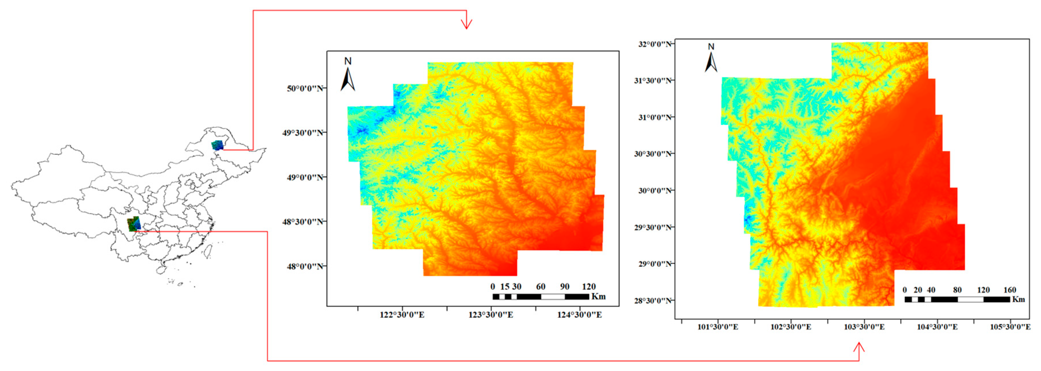
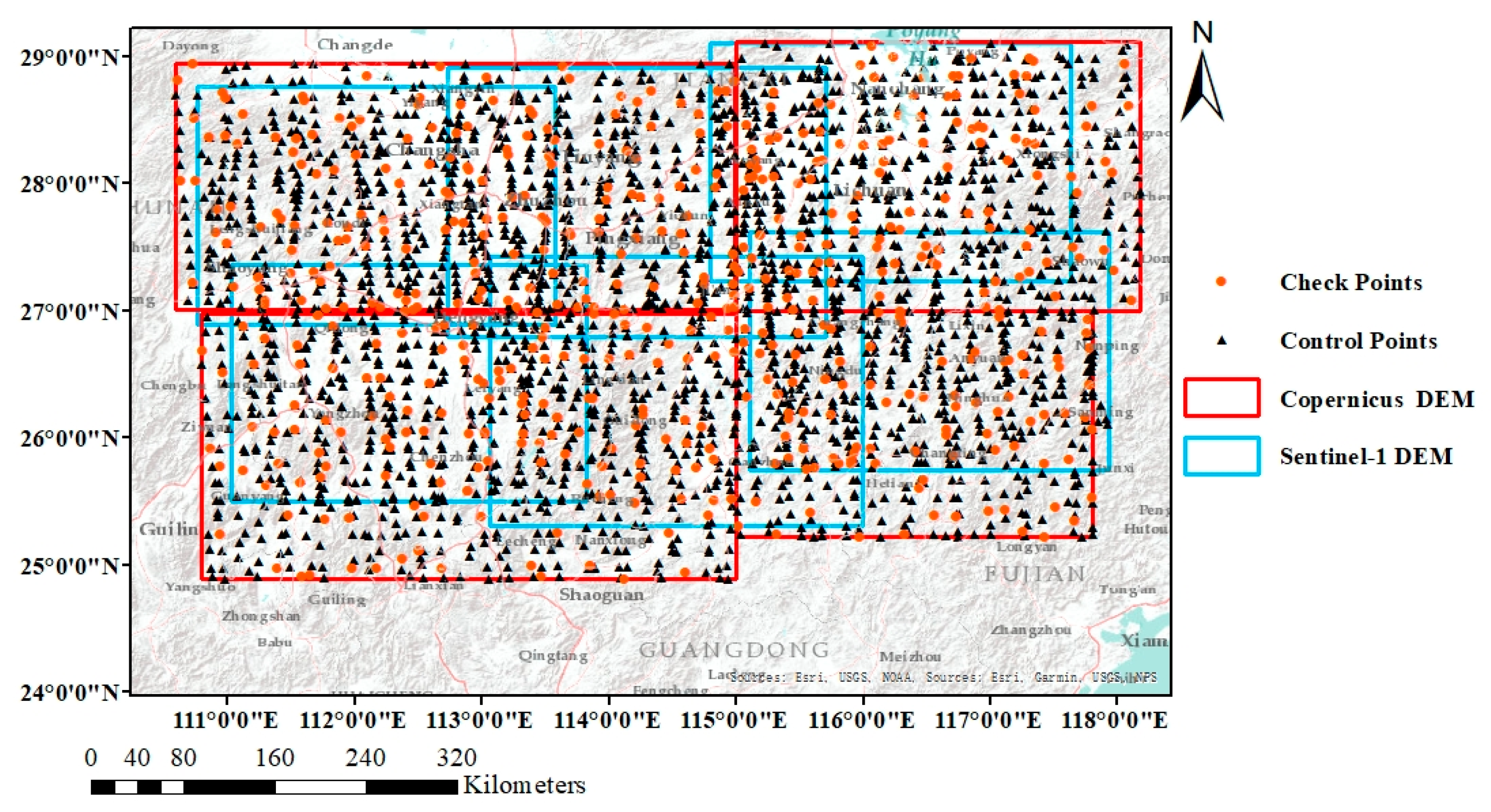
Research Region

To verify the effectiveness of the proposed InSAR-DEM tie point extraction and block adjustment methods, this study selects two regions with representative terrain characteristics in northern and southern China from the publicly available 12.5 m resolution InSAR-DEM data from ALOS PALSAR. The first dataset consists of 15 scenes covering the northeastern Daxing’an Mountains and the northern China Plain, located at the “first level terrace” of China’s topography. The geographic range of the data spans from approximately 47°52′35.0446″N to 50°17′31.1649″N, and from 121°52′35.0466″E to 124°46′03.8837″E, covering an area of approximately 56,418 km². The terrain is relatively flat, with an elevation range between 170 m and 1415 m. The second dataset consists of 30 scenes covering the DEM data of Sichuan Province in China, located at the “second level terrace” of China’s topography. The geographic range spans from approximately 28°23′49.9417″N to 32°01′32.4716″N, and from 101°31′50.9220″E to 104°52′29.3930″E, covering an area of approximately 129,830 km². The terrain is more varied, with an elevation range between 224 m and 7405 m. Detailed information about the study data is provided in

Table 1. Information of the research regions.

Research Region	Elevation Range	Area (km2)	Image Size (Pixels × Pixels)	Terrain
ALOS-PH	170–1415 m	56,418	17,424 × 20,907	Flat terrain and hills
ALOS-BP	224–7405 m	129,830	29,390 × 27,086	Mountains and basins

, and the geographical distribution of the study areas is shown in Figure 7. It should be noted that the original ALOS-DEM data are in UTM projection. To unify with the coordinate system of the ICESat-2 laser points, we reprojected the data from the UTM to the WGS84 coordinate system, and performed interpolation to ensure that the pixel resolution of the DEM remained consistent. In the following sections, we will refer to the first dataset as ALOS-PH(Plains and hills) and the second dataset as ALOS-BP(Basin and Plateau).

The main focus of the experiment is the InSAR-DEM TPs extraction method and the steps of three-dimensional registration adjustment that we proposed in the second section. It compares the error estimation capability of the extracted data and the qualitative and quantitative conditions before and after adjustment using a method based on sliding window matching InSAR-DEMs [12].

4. Results

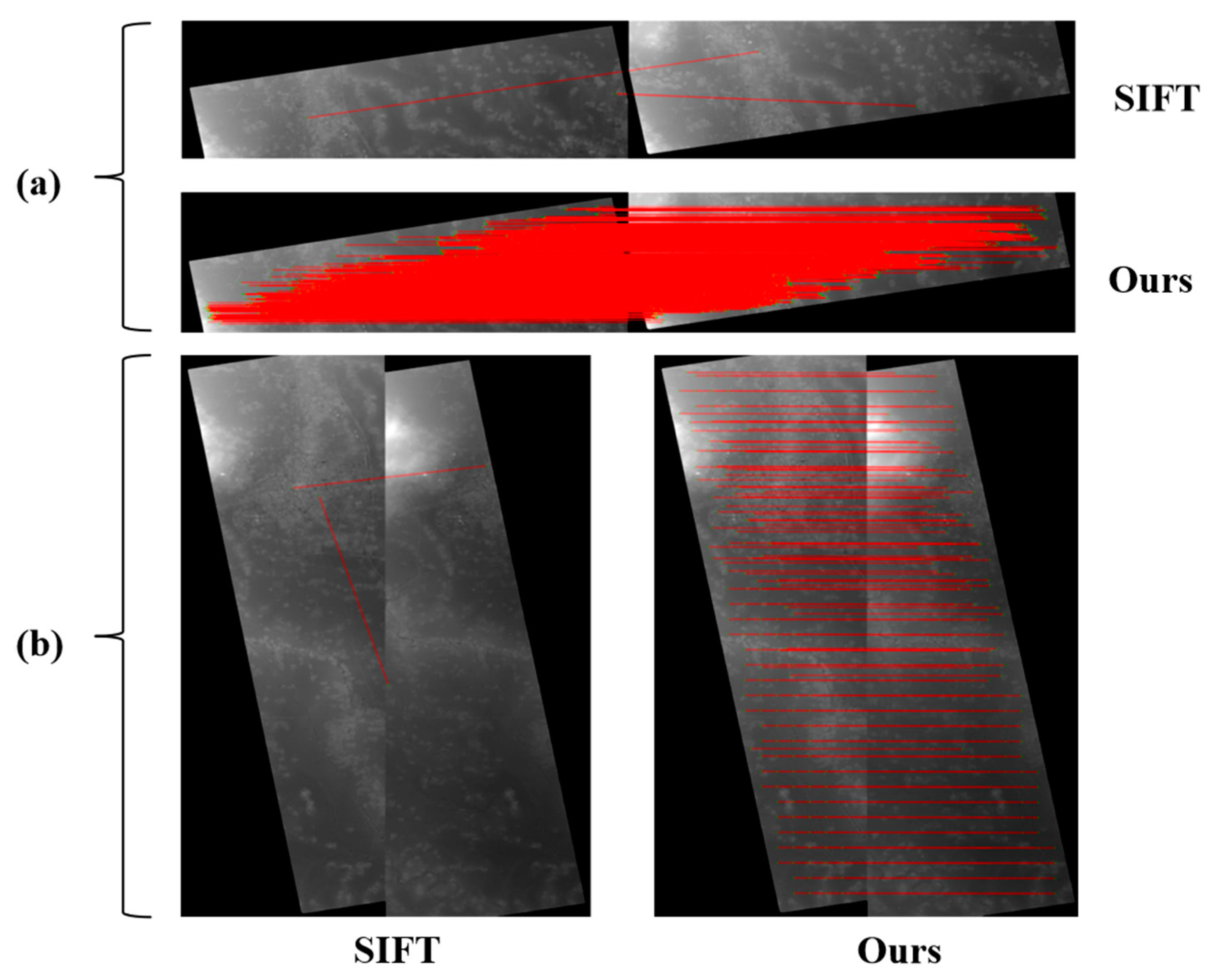
4.1. Keypoint Extraction and Matching

The first challenge in InSAR-DEM feature matching is that the DEM’s texture is weak, making it difficult to directly extract significant feature points. In Section 2, this paper fully considers the potential anomalies in the DEM and outlines a process aimed at enhancing and preserving the DEM’s feature texture. An adaptive threshold FAST detection method is proposed for feature point extraction in the DEM. In Figure 8, we present a set of feature point extraction results before and after InSAR-DEM feature processing, distinguishing between the along-track and cross-track directions.

In Figure 8, we can intuitively observe the significant difference in key point detection before and after our feature processing workflow. On the left side of the dividing line in Figure 8, it is nearly impossible to observe any features on the InSAR-DEM in flat terrain before the feature processing workflow. On the right side of the dividing line, after applying the proposed processing workflow, the features in the InSAR-DEM are noticeably enhanced. A comparison of the feature detection results is shown, with red, yellow, green, and blue windows representing local magnifications of the corresponding positions. For both before and after feature enhancement, we use the same locations for comparison. It can be seen that if no feature enhancement process is applied, the total number of identified feature points is significantly fewer than the result after the feature enhancement process. Moreover, directly detecting feature points on the unprocessed DEM will identify a large amount of noise as feature points. Such feature point detection results are disastrous for subsequent matching and adjustment tasks. After applying the proposed processing workflow, both the number of detected feature points and the quality of the extracted key points improve significantly compared to the pre-processing results. The quantitative metrics are provided in

Table 2. Quantitative results of key point extraction from InSAR-DEM before and after feature processing.

DEM Number	Orbital Position	Overlapping Area (Pixels)	Number of Points Before (Enhance)	Number of Points After (Enhance)
DEM-Figure 8a(left)	Along	$5668\times 1760$	5277	22,466
DEM-Figure 8a(right)	Along	$5668\times 1760$	5988	22,094
DEM-Figure 8b(left)	Vertical	$2704\times 7444$	21,237	56,318
DEM-Figure 8b(right)	Vertical	$2704\times 7444$	9541	78,174

.

After completing the key point localization, the 296-dimensional feature descriptor proposed in Section 2 is applied for matching. In Figure 9, the comparison results between the descriptor we proposed and the SIFT [25] algorithm are presented. It can be seen that under the same key point conditions, the SIFT descriptor is nearly unable to match InSAR-DEM key points, whereas the descriptor we proposed can robustly describe and match the DEM features. Due to the weak texture of the DEM, it is still difficult to visually observe the specific shapes of the matched feature points. However, a preliminary indication of the effectiveness of our proposed 296-dimensional multi-level centroid descriptor can be inferred from the comparison of the number and consistency of the matching lines. The specific matching accuracy will be further supported by more quantitative indicators in large-scale planar registration experiments. Further thoughts and discussions on the 296-dimensional DEM feature descriptor proposed in this paper can be found in the Discussion section.

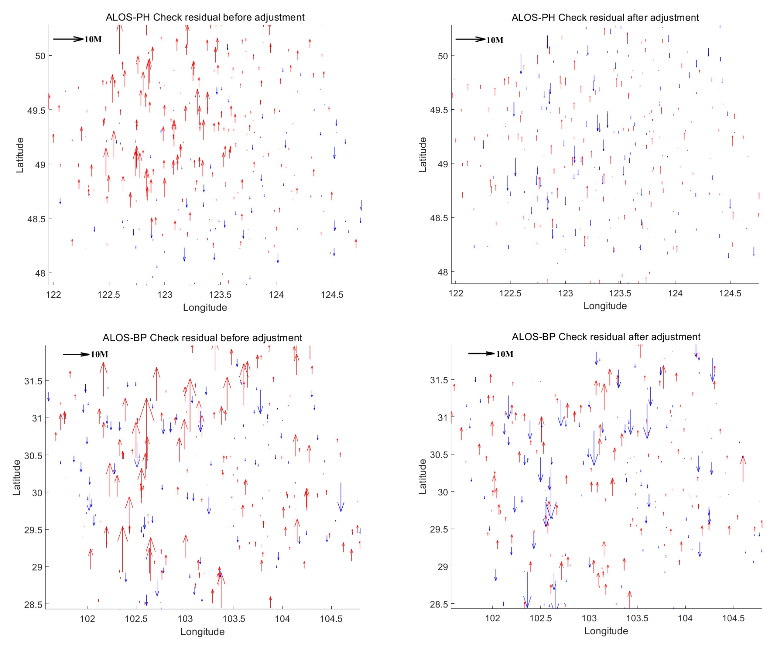
4.2. InSAR-DEM Block Adjustment Experiments and Comparisons

In this section, the proposed method is applied to large-scale DEM block adjustment tasks using the ALOS-PH and ALOS-BP datasets. In Figure 10, we show the distribution of TP detection results in the overlapping area of the ALOS-PH and ALOS-BP datasets. The blue points represent the location distribution of TPs on the DEM. After grid homogenization, a total of 6620 TPs were extracted from ALOS-PH, while a total of 9768 TPs were extracted from ALOS-BP.

In the InSAR-DEM elevation adjustment process, in addition to TPs, elevation control point data (HCPs) and check point data are also important. This paper uses the filtered ICESat-2 data and applies grid-based processing to evenly distribute elevation control points on both the ALOS-PH and ALOS-BP datasets. In addition to the evenly distributed control points, laser points that are as far as possible from the control points are selected as check data. The inspection points and control points for both experimental datasets are shown in Figure 11. The yellow dots represent elevation control points, while the red dots indicate inspection points.

Finally, on the ALOS-PH dataset, a total of 1330 elevation control points participated in the adjustment, and 333 elevation checkpoints were used for accuracy validation. On the ALOS-BP dataset, 2697 elevation control points were involved in the adjustment, and 277 checkpoints were used for accuracy validation. In

Table 3. Comparison of the relative planar registration quantitative results of ALOS-PH and ALOS-BP, along with a comparison of algorithm efficiency.

	After (m)	After (m)	After (m)	After (m)
Data	ALOS-PH	ALOS-PH	ALOS-BP	ALOS-BP
Method	sliding window	Ours	sliding window	Ours
X RMSE	2.656971	2.040121	2.166357	1.535620
Y RMSE	2.344169	1.910933	1.242834	0.910042
XY MEAN	2.798351	2.316631	1.723684	1.188659
The number of TPs	5363	6620	9414	9768
TPs matching time (second)	2106.27	2481.41	3967.8	4655.59

, we present the final results of the block adjustment for the two study areas, along with a comparison of the TPs extracted using the sliding window similarity-based InSAR-DEM matching method [12]. Meanwhile, we present the time consumption of the two methods in DEM feature matching in Table 3. Both the method proposed in this paper and the sliding window matching method utilize multithreading acceleration technology. Ultimately, our method took a total of 2481.41 s for matching on ALOS-PH data and 4655.59 s on ALOS-BP data.

Table 3 shows the results of relative plane registration using TPs. Due to the lack of real plane checkpoints, we conduct a quantitative assessment of the relative horizontal accuracy between TPs. The extraction methods for the two TPs differ, and thus the initial horizontal error detected by TPs varies significantly. To unify the evaluation standard, we use both TPs for plane registration of the DEM. After registration, we apply our proposed method for uniform matching, using the initial relative error of the match as a quantitative metric. It can be observed that the TPs extracted using our method estimate a better post-registration relative plane accuracy compared to the TPs extracted by the sliding window matching method. Our method improves the relative plane accuracy of ALOS-PH to 2.316631 m, which is about 0.4 m better than the 2.798351 m achieved by the sliding window DEM matching method. The relative plane accuracy of ALOS-BP is improved to 1.188659 m, while the sliding window DEM matching method reaches 1.723684 m. Comparatively, our proposed method improves plane consistency by about 0.52 m.

Table 4. Comparison of quantitative results of elevation adjustment between ALOS-PH and ALOS-BP.

	Before (m)	After (m)	After (m)	Before (m)	After (m)	After (m)
Data	ALOS-PH	ALOS-PH	ALOS-PH	ALOS-BP	ALOS-BP	ALOS-BP
Method	sliding window	sliding window	Ours	sliding window	sliding window	Ours
Height-ABS	2.156771	1.837497	1.729699	4.456939	4.293428	4.215460
Height-RMSE	3.086416	2.578077	2.268726	6.807942	6.435393	6.111026
Height-MAX	11.673828	9.721665	8.131412	35.339111	32.825108	30.146499
Height-MIN	0.001465	0.012924	0.014138	0.004364	0.006792	0.004192

presents the results of absolute elevation adjustment. As seen in the table, our method reduces the elevation error of ALOS-PH from 3.086416 m to 2.268726 m and the elevation error of ALOS-BP from 6.807942 m to 6.111026 m. In contrast, the sliding window matching method reduces the elevation error of ALOS-BP from 3.086416 m to 2.578077 m and the elevation error of ALOS-BP from 6.807942 m to 6.435393 m. In terms of the elevation adjustment results, the RMSE of our method is about 0.31 m better than the sliding window matching method for ALOS-PH data. The ABS index is improved by 0.11 m, and the maximum post-adjustment error is reduced by approximately 1.6 m. For ALOS-BP data, our method outperforms the sliding window matching method by about 0.325 m in elevation adjustment, with the ABS index improving by 0.08 m and the maximum error reduction of approximately 2.7 m. In the elevation adjustment experiment, we used the same HCPs and checkpoints, as well as the same adjustment model and weight settings. The only difference lies in the TPs used as control data. Therefore, we can conclude that the TPs extracted by our method perform better in terms of elevation accuracy compared to those proposed by the sliding window matching method. The following reasons support this conclusion: (1) Considering the data resolution of 12.5 m, the initial plane errors for both methods are within 1 pixel. The sliding window matching method, which uses elevation curve fitting to refine the TPs to sub-pixel accuracy, is less effective in flat regions. In areas with significant terrain variation, noise and fitting accuracy affect the results, limiting sub-pixel precision. In contrast, our method uses the FAST algorithm with an adaptive threshold to directly refine significant features on the DEM to sub-pixel accuracy, offering higher precision. (2) Due to the lack of real control points, the method we use to calculate plane accuracy involves computing the offset residuals between TPs before and after registration, which does not reflect the true error. As mentioned in the Introduction, baseline and viewpoint errors in the InSAR system cause non-uniform geometric distortions, which include not only horizontal shifts but also relative rotations and misalignments. The inherent characteristics of the sliding window similarity matching method lead to its poor sensitivity to geometric distortions when applied to DEM matching. Combining the results of the elevation adjustment, we can make a preliminary conclusion that our TPs extraction method outperforms the classic sliding window matching DEM method.

In the aforementioned large-scale InSAR-DEM registration adjustment experiment, it was demonstrated that the TPs extraction method proposed in this paper outperforms the currently mainstream sliding window DEM matching methods. However, we noted that the improvement in elevation adjustment results is not significant. As shown in Figure 12, the histogram indicates that the errors in the ALOS-PH data have decreased after adjustment, but the improvement is not significant. In contrast, the ALOS-BP data show a significant reduction in the initial maximum error and initial errors greater than 10 m after adjustment. However, for locations with initially small errors, the positional errors are difficult to correct, and there is even a slight increase in errors observed. In Figure 13, vector graphics are used to display the residual results before and after the adjustment of the two sets of data.

As can be seen in Figure 13, the residuals of the checkpoints before adjustment indicate that the elevation errors in both study areas improved after adjustment, but the improvement is not significant. The limited effectiveness of the adjustment is mainly due to the very complex initial elevation error situation of the ALOS data, especially in hilly terrain for ALOS-PH data and in plateau areas for ALOS-BP data. This complexity leads to a decreased fitting degree of the adjustment model to the errors. This phenomenon can be attributed to two main factors: (1) The ALOS data had already undergone elevation correction at the time of release, resulting in a very random error distribution. (2) In areas with steep terrain, the accuracy of elevation control points and checkpoints decreases compared to flat areas, leading to larger and more complex noise in hilly and plateau regions.

4.3. InSAR-DEM Block Adjustment

In order to further validate the effectiveness of the block adjustment model proposed in this paper, as well as the effectiveness of the proposed TPs extraction method in multi-source DEM matching tasks, we selected six uncorrected Sentinel-1 InSAR-DEM data scenes and their corresponding Copernicus InSAR-DEM (CopDEM) data for the next part of the heterogeneous DEM joint experiment. Among them, CopDEM serves as external reference data to provide additional absolute elevation accuracy control and extra absolute horizontal accuracy reference for Sentinel-DEM outside the laser elevation control points. As shown in Figure 14, Sentinel-1 covers parts of Fujian, Jiangxi, and Hunan provinces in China. The distribution of control and checkpoints is provided in Figure 14. The Sentinel-1 InSAR-DEM data were generated using publicly available Sentinel-1 imagery from ESA, with a resolution of 20 m, while the Copernicus InSAR-DEM is open-source data with a resolution of 30 m, offering relatively high elevation accuracy [37]. It is important to note that to ensure resolution differences do not affect the adjustment, we applied bilinear interpolation to resample the resolution of CopDEM data to 20 m. This process may cause a slight decrease in the absolute accuracy of CopDEM. A total of 2578 control points were involved in the adjustment, and 516 checkpoints were used for absolute accuracy verification.

TPs were extracted from the overlapping area of the Sentinel data and CopDEM. A total of 7069 pairs of TPs participated in the adjustment work.

Table 5. The results and comparisons of the joint planar registration of Sentinel and CopDEM are presented. The first two columns show the initial errors estimated by our method and the verification results, while the last two columns display the comparison results of the secondary matching after registration.

	Before	After (m)	After (m)	After (m)
Data	Sentinel	Sentinel	Sentinel (Second)	Sentinel (Second)
Method	Ours	Ours	sliding window	Ours
X RMSE	137.18337	6.660747	7.163181	6.844605
Y RMSE	32.527578	4.445506	5.002840	4.366544
XY MEAN	83.414873	5.876839	6.657243	5.713693

shows the results before and after planar registration. In the planar registration process, the relative geometric distortion between heterogeneous DEMs is much greater than that between homogeneous DEMs. The planar RMSE in the X direction before registration was 137.183370 m, and after registration, it was 6.660747 m. The planar RMSE in the Y direction before registration was 32.527578 m, and after registration, it was 4.445506 m. Overall, our method reduced the mean planar error from 83.414873 m to 5.876839 m. The error has decreased by approximately 93%. When converted to pixel space based on resolution, the planar relative error between CopDEM and Sentinel data improved from approximately 5 pixels to sub-pixel accuracy. Similarly, to compare with the currently classical sliding-window matching method and ensure the reliability of the comparison, the same method was applied after planar registration, as in Section 4.2. The initial error from the second matching step was used as the reference for relative horizontal error. After the second matching, the initial planar relative error of our method was 5.713693 m, with a difference of only about 0.1 m from the post-adjustment check results. This is better than the 6.657243 m result of the sliding-window similarity matching DEM method, which differs by approximately 1 m. This further proves that our method performs better than the sliding-window matching DEM method when dealing with significant geometric distortion.

Table 6. Sentinel and CopDEM elevation adjustment results.

	Before (m)	After (m)	Before (m)	After (m)	Before (m)	After (m)
Data	Sentinel& CopDEM	Sentinel& CopDEM	Sentinel	Sentinel	CopDEM	CopDEM
Height-ABS	14.611961	6.604417	19.352163	10.076845	10.490046	3.584915
HeightRMSE	19.018838	10.291855	24.362027	14.183206	12.655347	4.806659
HeightMAX	93.140530	68.818319	93.140530	68.818319	41.209506	25.76232
Height-MIN	0.0228270	0.0023850	0.0623359	0.0023850	0.0228269	0.052466

presents the elevation adjustment results, where the overall absolute elevation accuracy RMSE decreased from 19.02 m to 10.29 m, with a reduction rate of approximately 50%. The elevation RMSE for Sentinel data decreased from 24.36 m to 14.18 m, with an error reduction rate of approximately 41.8%. The elevation error RMSE for CopDEM data decreased from 12.66 m to 4.81 m, with an error reduction rate of approximately 62%.

Table 7. The ablation experiment compared the impact of joint adjustments on the absolute elevation accuracy of Sentinel data.

	Before (m)	After (m)	After (Without TPs)
Data	Sentinel	Sentinel	Sentinel
Height-ABS	19.352163	10.076845	10.627355
HeightRMSE	24.362027	14.183206	14.554168
HeightMAX	93.140530	68.818319	68.818319
Height-MIN	0.0623359	0.0023850	0.063000

shows the results of the ablation experiment on whether Sentinel-DEM is combined with CopDEM for joint elevation adjustment. It can be seen that after incorporating CopDEM for joint elevation adjustment, the absolute elevation accuracy of Sentinel-DEM improved by approximately 0.4 m, further demonstrating the practicality of the TPs extraction method proposed in this paper for matching heterogeneous DEMs.

The histograms of checkpoints before and after adjustment, as well as the residual plots, are shown in Figure 15 and Figure 16, respectively. In this set of experiments, the absolute elevation accuracy of CopDEM data was slightly better than 5 m but lower than its official reported accuracy. The result may be closely related to the resampling to a 20-m resolution. The qualitative results of Sentinel-DEM are presented in Figure 17. By observing the enlarged edges of the DEM, it can be seen that the originally misaligned peaks have been adjusted to form a cohesive whole, and the planar inconsistencies have significantly improved. For the adjusted Sentinel-DEM, we applied a weighted feathering mosaic algorithm [38] that distinguishes between orbital directions to achieve a smooth mosaic of the DEM edges. The edge conditions after mosaicking are shown in the corresponding position in Figure 17, where it can be seen that the seams between the DEM tiles have been further smoothed.

5. Discussion

This section discusses the selection of methods, method effectiveness, and parameter settings in the DEM feature processing workflow and TPs description matching.

(1)

Using the histogram of oriented gradients to describe features:

The most typical characteristic of DEM is weak texture. For matching issues with weak-textured remote sensing images, feature fusion in the spatial and frequency domains is an advanced method [39]. This paper adopts the concept of edge-preserving filtering in the spatial domain but does not perform feature processing on DEM in the frequency domain. The reason is that images primarily rely on optical or radar sensors for data acquisition, and these sensors capture images based on the physical principles of light or radar waves, which have wave-like physical properties. Therefore, phase consistency can be used to detect feature edges. A similar choice is made in feature description work. We refer to the GIFT descriptor structure, but instead of using multi-level Log-Gabor filter responses as sampling points [40], which are based on phase principles, we use orientation gradient histograms, which are more suitable for describing DEM features.

(2)

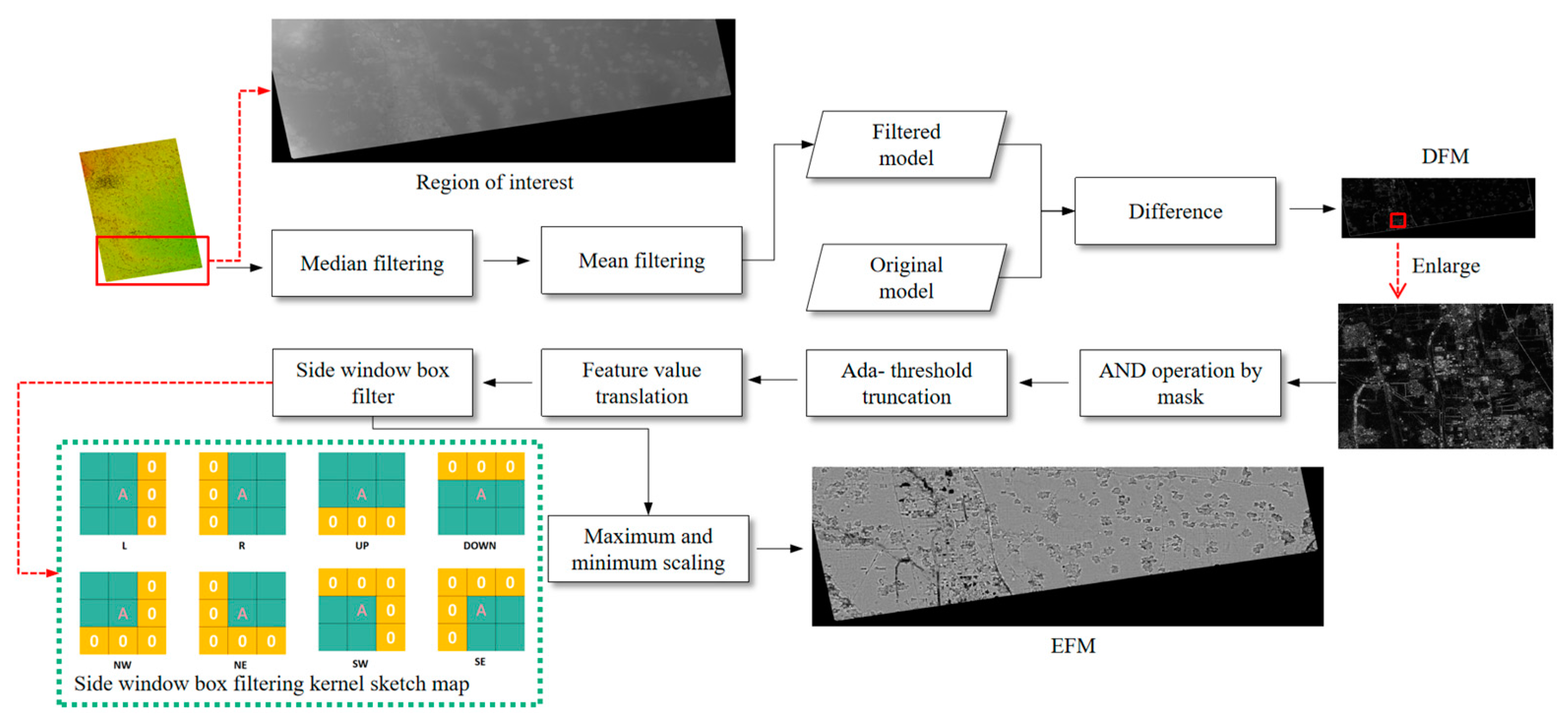
Selection of Filters: When selecting edge-preserving filters, the traditional edge-preserving filters include bilateral filtering, guided filtering, and weighted least squares filtering. The effectiveness of bilateral filtering is closely related to the thresholds in both the spatial and intensity domains, making it difficult to set effectively on BFI. When weighted least squares filtering is applied to BFI with pixel quantities in the tens of millions to billions, the size of the differential operator matrix can reach billions, resulting in an unacceptable computational burden. Guided filtering requires a guidance image as a reference, making it difficult to apply to BFI. Therefore, we use an improved box filter based on the side-window filtering principle to further remove chaotic textures while preserving edge characteristics.

6. Conclusions

This article mainly introduces a process for obtaining key control data (TPs) in the regional adjustment of InSAR-DEM using significant feature matching. By employing a framework based on significant feature matching, combined with feature enhancement and retention processes, adaptive feature point detection, and a 296-dimensional slope gradient feature descriptor with multi-level perception, high-quality tie points between DEMs are effectively detected. The method has been evaluated on large-scale DEM data. Conclusions can be summarized: (1) The DEM tie point extraction method based on significant feature matching can identify non-uniform geometric distortions between DEMs, and the accuracy of TPs extraction surpasses that of currently advanced sliding window-based DEM matching methods. (2) This method can effectively increase the number and accuracy of DEM feature point detection. Specifically, compared to directly using the FAST method, our method can increase the number of detected feature points by 4 to 10 times. (3) The proposed descriptor can directly describe DEM features rather than features of DEM-rendered images.

The limitation of this article lies in the fact that the results of matching cross-scale heterogeneous DEMs are currently quite average. The main reason may be that the differences in slope and aspect caused by the superimposition of elevation errors and texture differences at different resolutions lead to a lack of robustness in the feature descriptors. Future research will consider how to improve the robustness of descriptors during cross-resolution matching.

References

- Crosetto, M. Calibration and validation of SAR interferometry for DEM generation. ISPRS J. Photogramm. Remote Sens. 2002, 57, 213–227. [Google Scholar] [CrossRef]
- Gesch, B.; Muller, J.; Farr, T.G. The shuttle radar topography mission-Data validation and applications. Photogramm. Eng. Remote Sens. 2006, 72, 233. [Google Scholar]
- Wang, Q. Research on High-Efficiency and High-Precision Processing Techniques of Spaceborne Interferometric Synthetic Aperture Radar. Ph.D. Thesis, National University of Defense Technology, Changsha, China, 2011. [Google Scholar]
- Gonszález, J.H.; Bachmann, M.; Krieger, G.; Fiedler, H. Development of the TanDEM-X calibration concept: Analysis of systematic errors. IEEE Trans. Geosci. Remote Sens. 2009, 48, 716–726. [Google Scholar] [CrossRef]
- Curlander, J.C. Location of spaceborne SAR imagery. IEEE Trans. Geosci. Remote Sens. 1982, GE-20, 359–364. [Google Scholar] [CrossRef]
- Montazeri, S.; Rodríguez González, F.; Zhu, X.X. Geocoding error correction for InSAR point clouds. Remote Sens. 2018, 10, 1523. [Google Scholar] [CrossRef]
- Fisher, P.F.; Tate, N.J. Causes and consequences of error in digital elevation models. Prog. Phys. Geogr. 2006, 30, 467–489. [Google Scholar] [CrossRef]
- Gong, J.; Li, Z.; Zhu, Q.; Sui, H.; Zhou, Y. Effects of various factors on the accuracy of DEMs: An intensive experimental investigation. Photogramm. Eng. Remote Sens. 2000, 66, 1113–1117. [Google Scholar]
- Xijuan, Y.; Chunming, H.; Changyong, D.; Yinghui, Z. Mathematical model of airborne InSAR block adjustment. Geomat. Inf. Sci. Wuhan Univ. 2015, 40, 59–63. [Google Scholar]
- Wessel, B.; Gruber, A.; Huber, M.; Roth, A. TanDEM-X: Block adjustment of interferometric height models. In Proceedings of the ISPRS Hannover Workshop “High-Resolution Earth Imaging for Geospatioal Information”, Hannover, Germany, 2–5 June 2009; International Archives of the Photogrammetry, Remote Sensing and Spatial Information Sciences. pp. 1–6. [Google Scholar]
- Zhang, X.; Xie, B.; Liu, S.; Tong, X.; Ding, R.; Xie, H.; Hong, Z. A Two-Step Block Adjustment Method for DSM Accuracy Improvement with Elevation Control of ICESat-2 Data. Remote Sens. 2022, 14, 4455. [Google Scholar] [CrossRef]
- Hong, Z.-H.; Sun, P.-F.; Zhou, R.-Y.; Tong, X.-H.; Feng, Y.-J.; Liu, S.-J. Fast mosaicking method of InSAR-generated multi-stripe digital elevation model. J. Infrared Millim. Waves 2022, 41, 493–500. [Google Scholar]
- Wang, R.; Lv, X.; Zhang, L. A novel three-dimensional block adjustment method for spaceborne InSAR-DEM based on general models. IEEE J. Sel. Top. Appl. Earth Obs. Remote Sens. 2023, 16, 3973–3987. [Google Scholar] [CrossRef]
- Arefi, H.; Reinartz, P. Accuracy enhancement of ASTER global digital elevation models using ICESat data. Remote Sens. 2011, 3, 1323–1343. [Google Scholar] [CrossRef]
- Markus, T.; Neumann, T.; Martino, A.; Abdalati, W.; Brunt, K.; Csatho, B.; Farrell, S.; Fricker, H.; Gardner, A.; Harding, D. The Ice, Cloud, and land Elevation Satellite-2 (ICESat-2): Science requirements, concept, and implementation. Remote Sens. Environ. 2017, 190, 260–273. [Google Scholar] [CrossRef]
- Neuenschwander, A.L.; Magruder, L.A. Canopy and terrain height retrievals with ICESat-2: A first look. Remote Sens. 2019, 11, 1721. [Google Scholar] [CrossRef]
- Li, B.; Xie, H.; Liu, S.; Tong, X.; Tang, H.; Wang, X. A method of extracting high-accuracy elevation control points from ICESat-2 altimetry data. Photogramm. Eng. Remote Sens. 2021, 87, 821–830. [Google Scholar] [CrossRef]
- Moudrý, V.; Gdulová, K.; Gábor, L.; Šárovcová, E.; Barták, V.; Leroy, F.; Špatenková, O.; Rocchini, D.; Prošek, J. Effects of environmental conditions on ICESat-2 terrain and canopy heights retrievals in Central European mountains. Remote Sens. Environ. 2022, 279, 113112. [Google Scholar] [CrossRef]
- Li, B.; Xie, H.; Liu, S.; Xi, Y.; Liu, C.; Xu, Y.; Ye, Z.; Hong, Z.; Weng, Q.; Sun, Y. A high-quality global elevation control point dataset from ICESat-2 altimeter data. Int. J. Digit. Earth 2024, 17, 2361724. [Google Scholar] [CrossRef]
- Rosenholm, D.; TORLEGARD, K. Three-dimensional absolute orientation of stereo models using digital elevation models. Photogramm. Eng. Remote Sens. 1988, 54, 1385–1389. [Google Scholar]
- Streutker, D.R.; Glenn, N.F.; Shrestha, R. A slope-based method for matching elevation surfaces. Photogramm. Eng. Remote Sens. 2011, 77, 743–750. [Google Scholar] [CrossRef]
- Ravanbakhsh, M.; Fraser, C. DEM registration based on mutual information. ISPRS Ann. Photogramm. Remote Sens. Spat. Inf. Sci. 2012, 1, 187–191. [Google Scholar] [CrossRef]
- Li, Z.; Bethel, J. DEM registration, alignment and evaluation for SAR interferometry. Int. Arch. Photogramm. Remote Sens. Spat. Inf. Sci. 2008, 37, 111–116. [Google Scholar]
- Jurie, F.; Dhome, M. A simple and efficient template matching algorithm. In Proceedings of the Eighth IEEE International Conference on Computer Vision ICCV, Vancouver, BC, Canada, 7–14 July 2001; pp. 544–549. [Google Scholar]
- Lowe, D.G. Distinctive image features from scale-invariant keypoints. Int. J. Comput. Vis. 2004, 60, 91–110. [Google Scholar] [CrossRef]
- Bay, H.; Ess, A.; Tuytelaars, T.; Van Gool, L. Speeded-up robust features (SURF). Comput. Vis. Image Underst. 2008, 110, 346–359. [Google Scholar] [CrossRef]
- Li, J.; Hu, Q.; Ai, M. RIFT: Multi-modal image matching based on radiation-variation insensitive feature transform. IEEE Trans. Image Process. 2019, 29, 3296–3310. [Google Scholar] [CrossRef]
- Yao, Y.; Zhang, Y.; Wan, Y.; Liu, X.; Yan, X.; Li, J. Multi-modal remote sensing image matching considering co-occurrence filter. IEEE Trans. Image Process. 2022, 31, 2584–2597. [Google Scholar] [CrossRef]
- Hirt, C. Artefact detection in global digital elevation models (DEMs): The Maximum Slope Approach and its application for complete screening of the SRTM v4. 1 and MERIT DEMs. Remote Sens. Environ. 2018, 207, 27–41. [Google Scholar] [CrossRef]
- Hu, Z.; Gui, R.; Hu, J.; Fu, H.; Yuan, Y.; Jiang, K.; Liu, L. InSAR digital elevation model void-filling method based on incorporating elevation outlier detection. Remote Sens. 2024, 16, 1452. [Google Scholar] [CrossRef]
- Lecours, V.; Devillers, R.; Edinger, E.N.; Brown, C.J.; Lucieer, V.L. Influence of artefacts in marine digital terrain models on habitat maps and species distribution models: A multiscale assessment. Remote Sens. Ecol. Conserv. 2017, 3, 232–246. [Google Scholar] [CrossRef]
- Hirt, C.; Kuhn, M.; Claessens, S.; Pail, R.; Seitz, K.; Gruber, T. Study of the Earth’ s short-scale gravity field using the ERTM2160 gravity model. Comput. Geosci. 2014, 73, 71–80. [Google Scholar] [CrossRef]
- Huber, M.; Gruber, A.; Wessel, B.; Breunig, M.; Wendleder, A. Validation of tie-point concepts by the DEM adjustment approach of TanDEM-X. In Proceedings of the 2010 IEEE International Geoscience and Remote Sensing Symposium, Honolulu, HI, USA, 23–30 July 2010; pp. 2644–2647. [Google Scholar]
- Li, Z.; Shen, H.; Weng, Q.; Zhang, Y.; Dou, P.; Zhang, L. Cloud and cloud shadow detection for optical satellite imagery: Features, algorithms, validation, and prospects. ISPRS J. Photogramm. Remote Sens. 2022, 188, 89–108. [Google Scholar] [CrossRef]
- Koschan, A.; Abidi, M. Detection and classification of edges in color images. IEEE Signal Process. Mag. 2005, 22, 64–73. [Google Scholar] [CrossRef]
- Yin, H.; Gong, Y.; Qiu, G. Side window filtering. In Proceedings of the IEEE/CVF Conference on Computer Vision and Pattern Recognition, Long Beach, CA, USA, 15–20 June 2019; pp. 8758–8766. [Google Scholar]
- Marešová, J.; Gdulová, K.; Pracná, P.; Moravec, D.; Gábor, L.; Prošek, J.; Barták, V.; Moudrý, V. Applicability of data acquisition characteristics to the identification of local artefacts in global digital elevation models: Comparison of the Copernicus and TanDEM-X DEMs. Remote Sens. 2021, 13, 3931. [Google Scholar] [CrossRef]
- Datla, R.; Mohan, C.K. A novel framework for seamless mosaic of Cartosat-1 DEM scenes. Comput. Geosci. 2021, 146, 104619. [Google Scholar] [CrossRef]
- Zhang, Y.; Liu, T.; Cattani, C.; Cui, Q.; Liu, S. Diffusion-based image inpainting forensics via weighted least squares filtering enhancement. Multimed. Tools Appl. 2021, 80, 30725–30739. [Google Scholar] [CrossRef]
- Hou, Z.; Liu, Y.; Zhang, L. POS-GIFT: A geometric and intensity-invariant feature transformation for multimodal images. Inf. Fusion 2024, 102, 102027. [Google Scholar] [CrossRef]