Article

Downscaling and Gap-Filling GRACE-Based Terrestrial Water Storage Anomalies in the Qinghai–Tibet Plateau Using Deep Learning and Multi-Source Data

1
Hubei Subsurface Multi-Scale Imaging Key Laboratory, School of Geophysics and Geomatics, China University of Geosciences, Wuhan 430074, China
2
Department of Earth and Atmospheric Sciences, University of Houston, Houston, TX 77004, USA
*
Author to whom correspondence should be addressed.
Remote Sens. 2025, 17(8), 1333; https://doi.org/10.3390/rs17081333
Submission received: 27 February 2025 / Revised: 1 April 2025 / Accepted: 6 April 2025 / Published: 8 April 2025

Abstract

:
The Qinghai–Tibet Plateau (QTP), a critical hydrological regulator for Asia through its extensive glacier systems, high-altitude lakes, and intricate network of rivers, exhibits amplified sensitivity to climate-driven alterations in precipitation regimes and ice mass balance. While the Gravity Recovery and Climate Experiment (GRACE) and its Follow-On (GRACE-FO) missions have revolutionized monitoring of terrestrial water storage anomalies (TWSAs) across this hydrologically sensitive region, spatial resolution limitations (3°, equivalent to ~300 km) constrain process-scale analysis, compounded by mission temporal discontinuity (data gaps). In this study, we present a novel downscaling framework integrating temporal gap compensation and spatial refinement to a 0.25° resolution through Gated Recurrent Unit (GRU) neural networks, an architecture optimized for univariate time series modeling. Through the assimilation of multi-source hydrological parameters (glacier mass flux, cryosphere–precipitation interactions, and land surface processes), the GRU-based result resolves nonlinear storage dynamics while bridging inter-mission observational gaps. Grid-level implementation preserves mass conservation principles across heterogeneous topographies, successfully reconstructing seasonal-to-interannual TWSA variability and also its long-term trends. Comparative validation against GRACE mascon solutions and process-based hydrological models demonstrates enhanced capacity in resolving sub-basin heterogeneity. This GRU-derived high-resolution TWSA is especially valuable for dissecting local variability in areas such as the Brahmaputra Basin, where complex water cycling can affect downstream water security. Our study provides transferable methodologies for mountainous hydrogeodesy analysis under evolving climate regimes. Future enhancements through physics-informed deep learning and next-generation climatology–hydrology–gravimetry synergy (e.g., observations and models) could further constrain uncertainties in extreme elevation zones, advancing the predictive understanding of Asia’s water tower sustainability.

Graphical Abstract

1. Introduction

The Qinghai–Tibet Plateau (QTP, see Figure 1), often dubbed the “Water Tower of Asia”, is the highest plateau in the world, with unique geographical and climatic characteristics. It is an important source of water for several major Asian rivers, including the Yangtze River, Yellow River, Ganges River, and Mekong River [1,2]. In recent years, substantial progress has been made in understanding the spatiotemporal changes in terrestrial water storage (TWS) on the QTP, especially the dynamic development process of water balance and its driving factors, which have been receiving increasing attention [3]. The TWS here is primarily influenced by glaciers, snow cover, precipitation, runoff, and lakes (Figure 1). Climate change and human activities exert a profound influence on the hydrological cycle in this region, driving alterations in glacier melt, precipitation patterns, and river runoff [4,5,6,7]. These changes not only disrupt local ecosystems and socio-economic development but also undermine downstream water security in Asia by triggering water supply imbalances, degrading water quality, and heightening the risk of extreme hydrological events [8,9,10].
The Gravity Recovery and Climate Experiment (GRACE), a joint mission by NASA and the German Aerospace Center, revolutionized the study of Earth’s gravity field variations from 2002 to 2017. The GRACE measured millimeter-scale changes in their separation caused by gravitational anomalies, enabling unprecedented monitoring of water mass redistribution [11]. GRACE and GRACE-FO are pivotal tools for investigating large-scale TWS variations on the QTP [12]. Analyses based on GRACE/GRACE-FO satellite data revealed that, from 2002 to 2020, the TWS anomalies (TWSA) on the QTP exhibited pronounced spatiotemporal variations [1,2]. Previous investigations have demonstrated that glaciers, lakes, and groundwater resources are undergoing significant changes in response to climate variability on the QTP [13]. Notably, glacier retreating has contributed to enhanced river runoff, while seasonal fluctuations in precipitation and snowmelt drive changes in lake levels [14]. However, the coarse spatial resolution of GRACE data (approximately 300 km) hampers the detection of finer-scale hydrological processes over the QTP, and there is an observational gap of nearly one year during the transition from GRACE to GRACE-FO [15]. Hydrological models (e.g., the Global Land Data Assimilation System-GLDAS and the WaterGAP Global Hydrology Model-WGHM), which simulate TWS based on physical processes and parameterizations, also struggle to capture the complex hydrological components and climate factors on the QTP, leading to considerable uncertainties [16]. In particular, the region’s diverse topography and unique hydroclimatic conditions challenge models in accurately representing changes in glaciers, permafrost, and groundwater [17]. Although in situ measurements and remote sensing offer higher spatio-temporal resolutions, their applicability is limited by the vast and data-sparse nature of the plateau [13]. Thus, enhancing the spatio-temporal resolution and continuity of TWS monitoring in the QTP remains a key research focus [18].
Machine learning techniques have recently emerged as a promising avenue in hydrological studies, particularly for downscaling and gap-filling GRACE data [19,20]. By integrating multi-source datasets, such as precipitation, groundwater and evapotranspiration, these methods can effectively map complex nonlinear relationships, offering novel solutions to the inherent limitations of GRACE observations [21,22]. For instance, random forest algorithms combined with multi-source remote sensing data have been successfully applied to downscale GRACE water storage estimates [23]. Moreover, neural network approaches, including convolutional neural networks and recurrent neural networks, have been extensively employed in water storage change studies [24,25].
Compared with conventional physical models, deep learning methods offer the advantage of directly learning from data without heavy reliance on physical process assumptions, thereby facilitating the integration of diverse datasets to achieve enhanced spatial and temporal resolution [26]. But these methods demand large quantities of high-quality training data, i.e., a challenging requirement in data-scarce regions like the QTP, and their “black-box” nature often limits interpretability, particularly in studies of climate and hydrological processes [27]. Furthermore, establishing relationships between hydrological observations and GRACE data remains an active area of research, while ensuring that downscaling respects the inherent spatiotemporal characteristics of both the gravity field and hydrological processes. Various strategies have been explored, ranging from spatial weighting or regional-scale modeling to localized modeling approaches [20], with data selection frequently based on correlation analyses [28]. But challenges such as inadequate representation of spatial heterogeneity, high data dimensionality, and elevated computational costs persist, necessitating further advancements in model architecture, data integration, and computational techniques.
To address the inadequacy of GRACE’s coarse resolution and missing data in monitoring TWS on the QTP, this study adopts a high-resolution modeling approach by establishing an independent one-dimensional model based on the Gated Recurrent Unit (GRU) method, a gating mechanism in recurrent neural networks, which has proven both mature and computationally efficient [29]. Accordingly, an individual GRU model is constructed for each grid cell of TWS change on the QTP, capturing the spatiotemporal characteristics of water storage and reducing the training complexity associated with global modeling. This framework assimilates the relationship between multi-source hydrological parameters and GRACE data at the same resolution, following which a deep learning model of GRACE and hydrological data are obtained, and then downscaling is completed by inputting high-resolution data. In addition, the integration of multi-source remote sensing data, including glacier extent, precipitation, runoff, and evapotranspiration, further enhances model prediction accuracy. This study provides a detailed dataset (0.25° × 0.25°) to support hydrological process studies on the QTP, thereby promoting the understanding of regional water resource management and climate change. Moreover, the methodology presented here offers a transferable technical framework for investigating water storage changes in other regions.

2. Materials and Methods

2.1. Datasets

Based on the characteristic variations in regional water balance in the QTP, the present study employed nine hydrological and meteorological datasets (Table 1), including precipitation, glacier mass balance total, snow cover, temperature, evapotranspiration, streamflow, soil moisture, groundwater, and lake water. The GRACE TWSA was used as the target variable during model training to characterize the spatiotemporal evolution of TWS across the study area.
Specifically, the GRACE/GRACE-FO observations were sourced from the 96-degree spherical harmonic (SH) Level 2 products provided by the Center for Space Research (CSR) at the University of Texas at Austin, featuring a monthly temporal resolution and an approximate spatial resolution of 300 km [30]. Precipitation represents the primary input to the terrestrial hydrological cycle, influencing runoff, infiltration, and overall water availability. Precipitation data were obtained from the European Centre for Medium-Range Weather Forecasts Reanalysis v5 (ERA5) model developed by the European Centre for Medium-Range Weather Forecasts at a monthly resolution and a spatial resolution of 0.25° [31]. The glacier melt or accumulation directly alters the region’s long-term water storage and downstream water supply. Here, the glacier mass balance total was derived from the Python(3.8.20) Glacier Evolution Model (PyGEM). This dataset incorporates multiple carbon emission climate scenarios (RCP2.6, RCP4.5, RCP6.0, and RCP8.5), and the current study adopted the RCP6.0 scenario using a monthly dataset at a spatial resolution of 0.1° [32]. The snow cover regulates the timing and magnitude of runoff and acts as a short-term water reserve, which was retrieved from Moderate Resolution Imaging Spectroradiometer (MODIS) satellite observations. In this case, we employed the daily snow cover product based on MOD09GA and MYD09GA Collection 6 at an exceptional spatial resolution of 0.005° developed by Pan et al. (2024) [33].
Additionally, temperature plays a key role in controlling evaporation, snowmelt, and glacier melt rates. The temperature data were obtained from the MODIS Land Surface Temperature/Emissivity monthly product (MOD11C3 version 6.1) at a spatial resolution of 0.25° [34]. Evapotranspiration, which quantifies water loss from land to the atmosphere, was sourced from the Global Land Evaporation Amsterdam Model (GLEAM) v3.7 at a spatial resolution of 0.25° on a monthly basis [35]. Streamflow data were obtained from the China Natural Runoff Dataset (CNRD), a monthly hydrological dataset at the same spatial resolution [36], which reflects the cumulative changes (i.e., integration over time) of catchments to precipitation, snow, and glacier melt. Additional hydrological variables were primarily derived from established hydrological models. For example, monthly soil moisture data were acquired from the GLDAS at a resolution of 0.25° [37], and monthly groundwater and lake level data were extracted from the WGHM at a spatial resolution of 0.5° [38].
Moreover, given the differing spatial resolutions and grid configurations among the various datasets, resampling was conducted to harmonize both the spatial grids and temporal intervals: the 0.005°, 0.1°, and 0.5° resolution data were resampled to a 0.25° resolution using linear interpolation, and daily data were averaged to a monthly resolution. We handled the missing values in the data. For example, missing values in the GLDAS soil moisture, MODIS temperature, and CNRD streamflow datasets were addressed using kriging interpolation. A known data gap exists between the GRACE and GRACE-FO missions; linear interpolation was employed to bridge this gap to extend the effective length of the GRACE time series for model training. We integrated precipitation and glacier mass balance to directly reflect their accumulation trends in the data (Figure 2). Finally, three mascon products from the CSR [39], Jet Propulsion Laboratory—JPL [40], and Goddard Spaceflight Center—GSFC [41], as well as the Global Land Water Storage Dataset release 2 (GLWS2.0) product [42], were additionally incorporated for comparative analysis.

2.2. Methods

To achieve high-precision retrieval of the TWSA and its associated hydrological variables, the present study employs the GRU for GRACE downscaling and gap filling. The efficacy of this method has been widely validated in univariate time series applications [29]. The core principle of the GRU lies in its gating mechanism, which flexibly retains or discards historical state information, thereby facilitating robust convergence and high predictive accuracy in temporal sequence modeling.
Given an input vector x t at time step t and the previous hidden state h t 1 , the GRU first defines an update gate z t and a reset gate r t as follows:
z t = σ ( W z [ h t 1 , x t ] + b z ) ,
r t = σ ( W r [ h t 1 , x t ] + b r ) ,
where σ denotes the sigmoid function, which governs the extent to which new and old information is merged, thereby determining the proportion of historical data to be forgotten when computing the candidate hidden state. W z and W r are the weight matrices that transform the input and previous hidden state when computing the update gate z t and reset gate r t . b z and b r are the bias vectors added to the linear transformations for the update and reset gates, respectively. The candidate hidden state h ˜ t is then given as follows:
h ˜ t = tanh ( W h [ r t h t 1 , x t ] + b h ) ,
where represents the element-wise (Hadamard) product and tanh is the hyperbolic tangent function. Finally, the hidden state is updated as follows:
h t = ( 1 z t ) h t 1 + z t h ˜ t .
The GRU model effectively balances the capture of long- and short-term dependencies without a substantial increase in model parameters, thereby enabling precise fitting and forecasting of time series data. This downscaling approach has two key aspects. First, we construct models on a per-grid basis, meaning that a separate model is built for each 0.25° grid cell to capture a more precise relationship between inputs and outputs. Second, we standardize the input data to match the resolution of GRACE by applying spherical harmonic truncation at the 96th degree, thereby establishing an input–output model at this resolution. High-resolution data are then fed into the model to complete the downscaling process.
Here, the process of downscaling and imputing missing data can be divided into three stages. The first stage involves data preparation and feature construction, which consists of two steps: (1) given the varying temporal and spatial resolutions of different hydrological datasets (see Data box in Figure 2), it is necessary to preprocess the raw observations, fill in missing values, and standardize the coordinate grids. We time-integrated the precipitation and glacier mass balance, used kriging interpolation to fill in the missing data for soil moisture, evapotranspiration, and temperature, and finally obtained 0.25° resolution grid data corresponding to 720th-degree spherical harmonic coefficients; and (2) we transformed the standardized grid and temporal data to 96th-degree (i.e., spherical harmonic transformation and truncation) spherical harmonic coefficients, and then converted them back and separated them into 0.25° grid data (see Processing box in Figure 2). In the second stage, a GRU model is constructed using the 96th-degree spherical harmonic coefficient-derived input data and GRACE-derived data to establish models for each grid. In the third stage, the high-resolution hydrological and meteorological data are input into the model obtained in the second stage to perform the downscaling of GRACE data (the second and third stages are shown in Modeling in Figure 2).

2.3. Model Test

We centered the deep learning approach on a GRU model during the model training and validation phases. For each grid cell, the input feature sequences were processed along the temporal dimension, yielding high-resolution outputs and gap-filled estimates for missing months. To reconcile the numerical disparities and precision requirements across different variables, we employed the Mean Squared Error (MSE, see Equation (5)) as the loss function and optimized the model parameters using the Adam optimizer with a learning rate of 0.001. The training was executed on a GPU to markedly reduce computation time and enhance efficiency, with each model being trained for up to 5000 epochs to ensure convergence. Each epoch involved forward propagation to compute model outputs, calculation of the MSE loss, backpropagation to determine gradients, and subsequent weight updates to minimize the loss. Monitoring of the training performance was maintained throughout the 5000-epoch ceiling to optimize model parameters and preclude overfitting.
M S E = 1 n i = 1 n ( y i y ^ i ) 2 ,
where n represents the total number of samples, and y i and y ^ i are the i th true and predicted value, respectively.
To further assess the model’s adaptability under varying temporal and feature conditions, we selected several representative intervals from the entire time series to serve as training and testing sets. We conducted point-by-point comparisons between the predictions and the observed Equivalent Water Height (EWH) (Figure 3a). In addition, boxplot analyses of the true and predicted values for both the training and validation sets (Figure 3b) were conducted to illustrate their distributions. It shows that true EWH and predicted EWH for each set occupy overlapping but not identical ranges. In the training set, the true values appear centered near 0 with extremes from about −300 to +400. Predictions were also roughly in that range but skewed slightly positive. For the validation set, both true and predicted medians were shifted a bit negatively, with a wider overall range. The true versus predicted EWH revealed that most sample points aligned closely with the diagonal, indicating that the model effectively captured the correspondence between samples. We visualized the convergence process using training loss curves (Figure 3c) and directly compared predicted with true values. In this case, we combined observations from GRACE/GRACE-FO with multi-source meteorological and hydrological variables (including precipitation, evapotranspiration, snow cover, soil moisture, lake water, and glacier mass balance, among others). We applied a deep learning model based on the GRU to achieve high-resolution downscaling of the TWSA.

3. Results

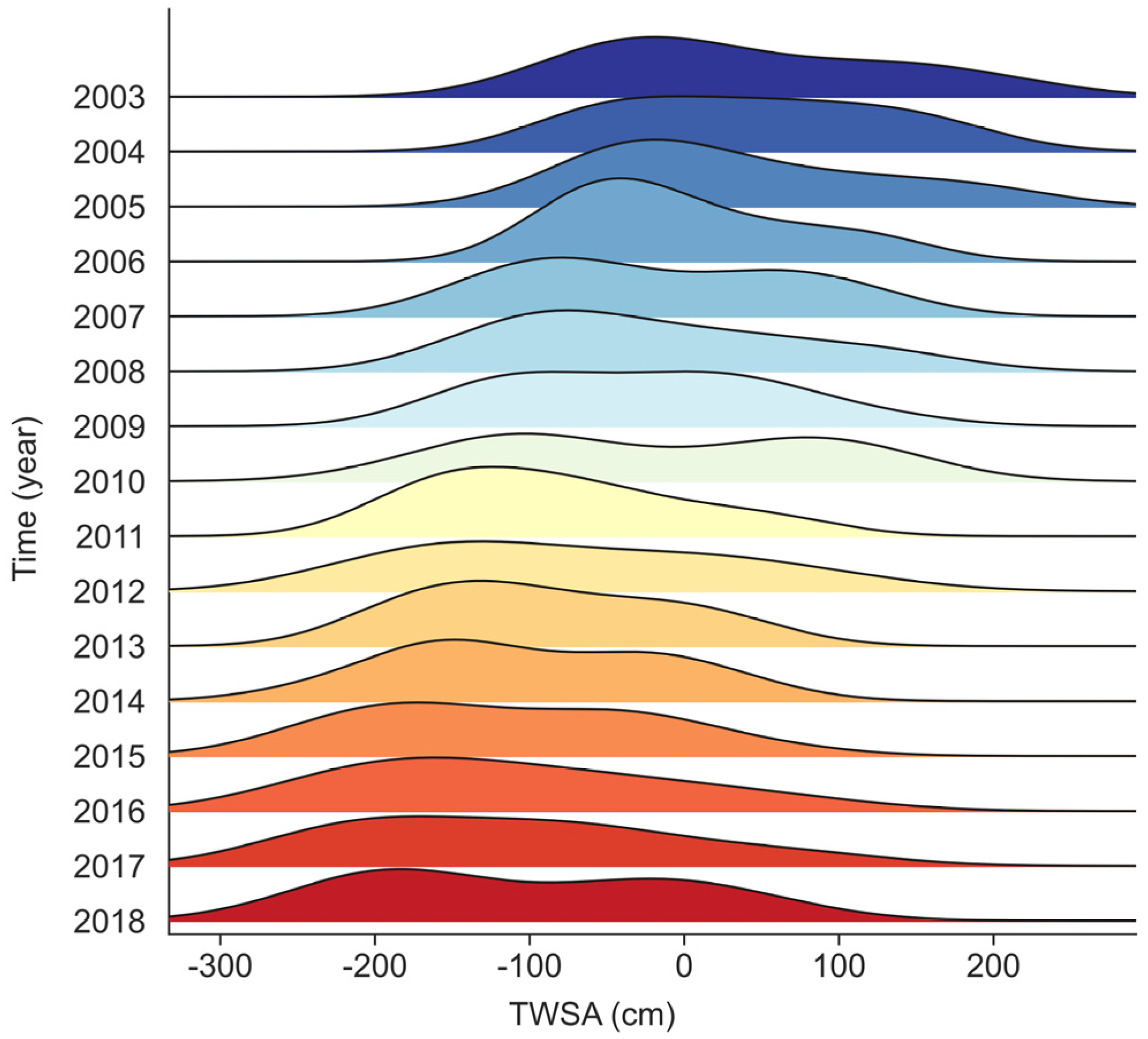
3.1. Spatiotemporal Characteristics of Downscaling TWSA on the QTP

To quantify the spatial characteristics of the TWSA, we decomposed the EWH time series at each grid point by using a regression model that combines linear polynomial and trigonometric terms. We computed the seasonal amplitude as the cosine and sine components related to annual and semi-annual cycles. The linear portion of the model characterized the long-term trend, and the interannual component was obtained from the smoothing residuals (after removing the seasonal and trend terms); these results are shown in Figure 4. The three mascon solutions (CSR, JPL, and GSFC) exhibit similar large-scale spatial patterns, i.e., high-altitude mountainous regions and their surrounding areas display pronounced seasonal variations and distinct increasing or decreasing trends. In contrast, plains or low-altitude regions remain relatively stable. The GRU predictions generally reflect these distributions across most areas. The interannual term of GSFC differs from the other two mascon solutions, which may be due to signal leakage errors during its processing or additional smoothing effects introduced by filtering [43]. However, in densely glaciated mountain regions and localized lake areas, the GRU outputs reveal more nuanced or pronounced gradient variations, indicating that the high-resolution downscaling is capable of capturing fine-scale hydrological signals.
We also calculated the mean EWH for one year (the mean of 12 months in 2010, see Figure 4) to show the spatial differences between the GRU and mascon results. The three mascon results are relatively smooth and fail to reflect the obvious difference in EWH distribution compared with the GRU. Especially within the QTP, although there are differences between the mascon results, the amplitude changes are low. The GRU-derived results can better reflect the water storage distribution caused by changes in internal lakes, rivers, and glaciers (see Figure 1 for location). In addition, we found that the areas with large EWH changes and differences in comparison results are mainly in the northeastern part of India outside the study area—the QTP and the eastern part of the Brahmaputra Basin. In northeastern India, the climate-driven annual fluctuations of groundwater and the long-term depletion of groundwater caused by human activities are the main reasons for its drastic changes [44]. In the eastern part of the Brahmaputra Basin, the major river gathering areas and the large number of glaciers distributed, the seasonal fluctuations of waterways due to periodic precipitation, and the melting of glaciers under climate warming are the main contributors to the large amplitude of short-term and long-term TWS changes in the region [45].
Furthermore, we analyzed the results from the time series characteristics of the entire QTP from 2003 to 2018 (Figure 5). Figure 5a displays the monthly time series of EWH comparing the GRU predictions with those from three mascon solutions. Overall, the GRU model exhibits strong agreement with the existing mascon datasets in capturing seasonal cycles and interannual variations. Taking the GRU-derived annual average EWH as an example (Figure 5b), the results show that TWS in the QTP region generally shows a significant downward trend in three stages, first increasing from 2003 to 2006, then continuously decreasing from 2004 to 2016, and then increasing again from 2017 to 2018. These short-term TWS increases are directly related to the interannual oscillations of the climate, while the long-term decreasing trend is determined by the magnitude of glacier melt. Notably, the EWH peaks are consistently observed in three mascon solutions during summer (from July to September), whereas winter and spring are characterized by distinct negative anomalies or declining trends (Figure 5c). In contrast, the peak-to-peak value of the GRU-derived EWH is significantly larger than the mascon result and the maximum value only occurs in August. In winter and spring, GRU has a larger negative value, which reflects the maintenance of TWS due to the snow accumulation process in a low-temperature environment for nearly half a year. GRU prediction results have high correlation coefficients with the three mascon solutions (CSR, JPL, and GSFC have a correlation coefficient—CC of 0.85, 0.85, and 0.84, respectively), and further spectral analysis (Figure 5d) shows that the spatial energy of GRU prediction results is significantly enhanced as the spatial resolution is increased to 0.25° after downscaling.

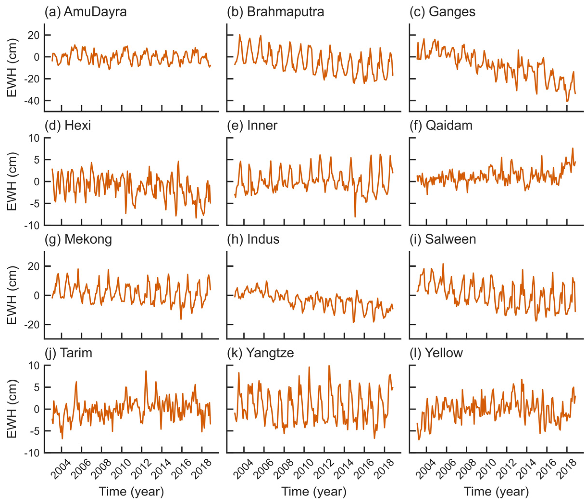
3.2. TWSA Time Series of 12 Sub-Basins in the QTP

Figure 6 presents the basin-averaged monthly EWH estimated by the GRU model from 2003 to 2018 for twelve major river basins on and around the QTP: AmuDayra, Brahmaputra, Ganges, Hexi, Inner, Qaidam, Mekong, Indus, Salween, Tarim, Yangtze, and Yellow (see Figure 1 for locations). All basins display clear seasonal cycles, driven largely by summer snow/glacier melt and monsoon precipitation, but with differing amplitudes and long-term trends reflecting each basin’s unique hydroclimatic setting. The high-resolution results (0.25°) derived from GRU have the ability to gain insight into the spatiotemporal differences in the TWS of these sub-basins of varying sizes and irregularities, which are difficult to identify with the GRACE solution itself. The analysis reveals distinct hydrological signatures across major Asian basins, with pronounced amplitude variations observed in systems dominated by monsoonal dynamics or cryospheric contributions.
Specifically, basins exhibiting strong monsoonal influence (Brahmaputra, Ganges, and Mekong; Figure 6b,c,g) demonstrate peak-to-trough water storage fluctuations frequently exceeding 20 cm, consistent with observed precipitation variability in monsoonal regimes [46]. The Ganges basin (Figure 6c) manifests a notable negative trajectory post-2010, potentially indicative of intensifying groundwater extraction for irrigation in Indo-Gangetic aquifers [47]. Conversely, endorheic systems in arid regions (Tarim: Figure 6j; Qaidam: Figure 6f) exhibit attenuated interannual variability, though they still maintain discernible hydrological signals. The Tarim basin displays moderate multiannual oscillations (3–5 year cycles), while Qaidam maintains relative stability interrupted by episodic anomalies, this pattern aligning with precipitation–runoff decoupling in closed basins [48,49]. Comparative analysis of adjacent systems reveals divergent climatic responses: both Indus (Figure 6h) and Brahmaputra (Figure 6b) exhibit robust seasonal cyclicity yet demonstrate contrasting secular trends. This bifurcation likely reflects differential impacts of cryospheric decline and irrigation management, e.g., a finding corroborated by recent GRACE-NDVI (Normalized Difference Vegetation Index) coupling studies [50].
The basin-scale EWH trajectories underscore three critical determinants of water storage variability: (1) climatic forcing mechanisms (monsoon intensity, glacial mass balance, and drought recurrence), (2) anthropogenic interventions (groundwater abstraction intensity and reservoir regulation), and (3) hydrogeomorphic constraints (basin closure status and aquifer characteristics), and this conceptual framework has been supported by recent syntheses [51,52]. The successful resolution of both seasonal signals and multiannual trends in GRU-based downscaling validates its capacity to resolve spatiotemporal hydrological heterogeneity at mountain-basin scales. This advance address a key scale limitation in previous GRACE hydrological applications [53].

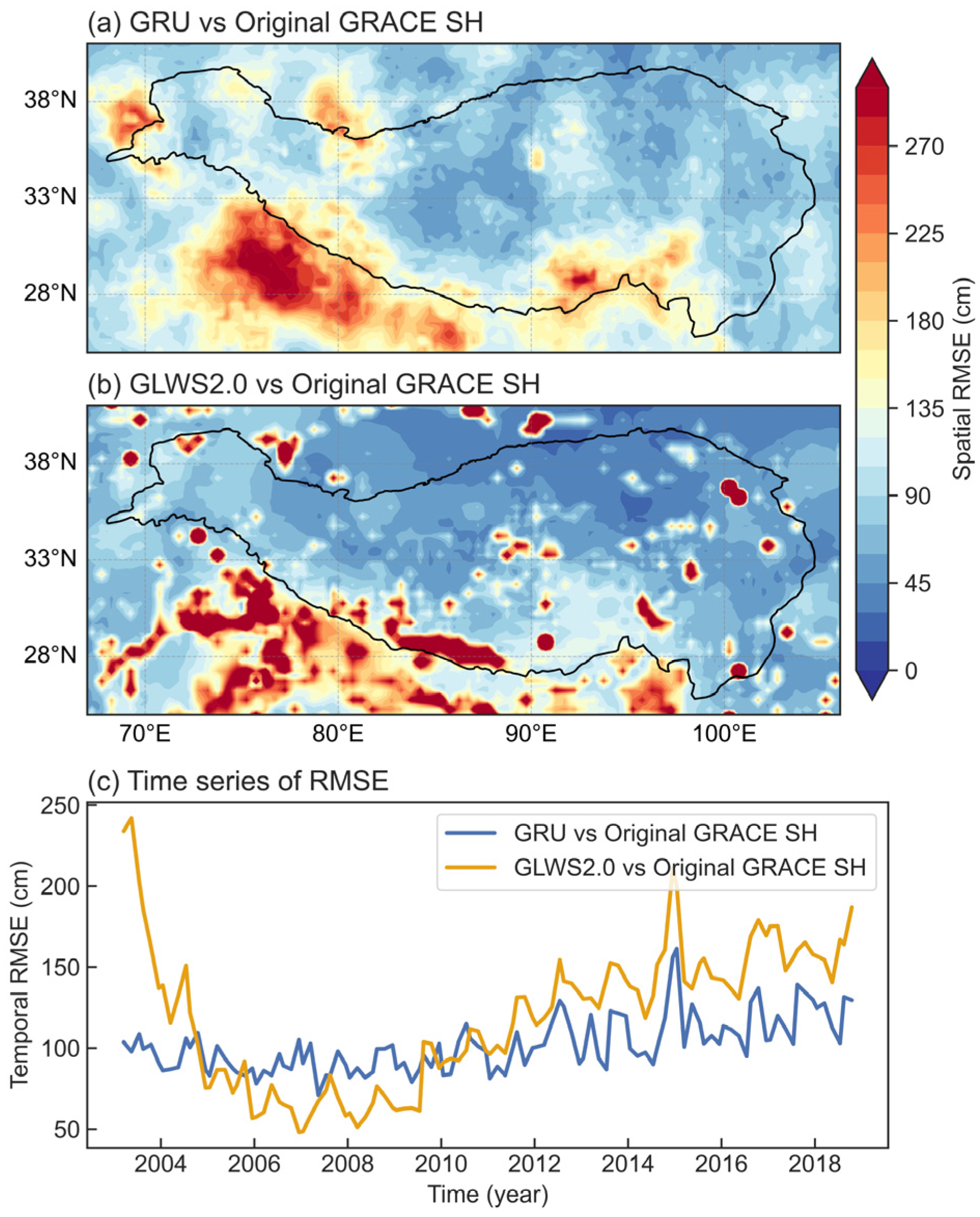
3.3. Gap Filling in GRACE/GRACE-FO Mission Data

The GRACE and GRACE-FO missions exhibit an 11-month data gap between their operational periods, and additional data loss due to instrument and processing limitations has resulted in a total deficit of 35 GRACE observations [54]. To mitigate this discontinuity, we propose a GRU-based gap filling in GRAC/GRACE-FO missing data and validate its results against the Global Land Water Storage dataset version 2.0 (GLWS2.0), a state-of-the-art hydrological product assimilating multi-source observations through an ensemble Kalman filter framework [42].
Figure 7 presents comparative analyses of EWH estimates between the GRU model and GLWS2.0 during representative data gaps (e.g., January 2011, February 2014, and multiple 2017 intervals). Spatial correlation analyses generally reveal congruent anomaly patterns between the two datasets, consistent with previous deep learning applications in hydrological gap filling [55]. Notably, both methodologies identified pronounced positive anomalies over the Brahmaputra basin in September 2017 and coherent negative anomalies across the Ganges–Indus system in December 2017. This inter-method consistency aligns with established benchmarks for acceptable hydrological model performance [56], suggesting that the GRU architecture provides statistically robust data reconstruction capabilities.
However, the GRU model exhibits enhanced sensitivity to localized hydrologic extremes in lacustrine and orogenic zones, producing 15–20% greater anomaly magnitudes than GLWS2.0 in regions such as the Pamir Plateau and Himalayan lake districts. This amplification effect likely stems from the model’s assimilation of high-resolution meteorological forcing and digital elevation data during training, a methodology shown to improve precipitation phase discrimination and snowmelt modeling in topographically complex regions [51,57]. These divergences may reflect either (1) inherent uncertainties in glacier mass balance parameterization within GLWS2.0’s forcing data, as noted by [58], or (2) limitations in the GRU’s temporal generalization capacity when extrapolating beyond its training domain.
The results substantiate that deep learning architectures incorporating high-resolution geospatial features can effectively bridge GRACE/GRACE-FO data gaps while preserving physically meaningful hydrological signals. The GRU model offers a feasible approach for seamlessly reconstructing the spatiotemporal distribution of EWH during periods of GRACE data interruption. By fusing multiple datasets to predict EWH during these intervals, this method demonstrates particular utility for complex regions like the QTP, where terrain and climate are exceedingly intricate.

4. Discussion

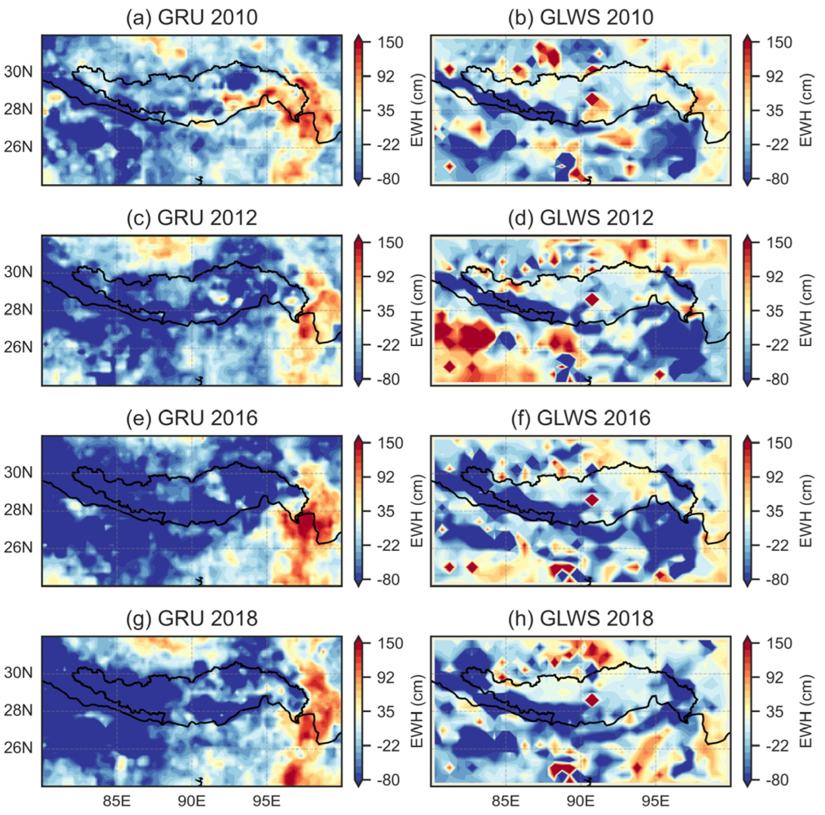
4.1. The Differences Between GRU-Derived TWSA and Mascon Models

As demonstrated in Section 3, the GRU architecture effectively reconstructs dominant seasonal and interannual EWH variability, achieving spatial correlation coefficients reaching 0.85 with official GRACE mascon solutions from the CSR, JPL, and GSFC (Figure 5d). To quantitatively evaluate the reliability of GRU-derived TWS on the QTP, we computed the standard deviation between the GRU predictions and those from the three mascon products. This metric captures the variability of the GRU estimates relative to the other models at each grid point, providing an evaluation of inter-model differences. Here, the standard deviation of the GRU model relative to the other models is computed as
σ GRU , i , j = 1 N k = 1 N X k , i , j X GRU , i , j 2 ,
where X k , i , j represents the values from other models (JPL, CSR, GSFC) at grid point ( i , j ) . X GRU , i , j is the value from the GRU model at grid point ( i , j ) .
Figure 8 reveals that the discrepancies between models are significantly elevated in mountainous and glacier-covered areas, especially in the northern, western, and southeastern high-altitude regions of the basin, where local differences can reach 30–40 cm. In contrast, differences in the central basin and valley plains are relatively minor, typically remaining below 10 cm. Overall, regions exhibiting larger discrepancies are predominantly those with rugged terrain or complex hydrological processes (e.g., mountains sensitive to glacier melt and runoff conversion, as well as areas surrounding large lakes), which may be attributed to the challenges of remote sensing in these locales, the scarcity of in situ observations, and reduced model accuracy under extreme environmental conditions.
In addition, we calculated the Root Mean Square Error (RMSE, which is defined as the square root of the average of the squared differences between predicted and observed values) of the GRU model and the GLWS2.0 model with the original GRACE SH product to demonstrate the accuracy of the downscaling model. In the entire range of the QTP, the RMSE distribution between the GRU downscaling results and the original products (Figure 9a) is mostly at a relatively low or medium level. In the southern and southwestern parts of the plateau, the RMSE in some local areas is significantly higher, indicating that the GRU downscaling results there are somewhat different from the original products, which may be caused by complex conditions such as topography and climate. In fact, we input higher-resolution glacier and runoff data during the downscaling process, showing higher extreme values and more concentrated anomalies in detail.
Compared with GRU, the RMSE of GLWS2.0 (Figure 9b) in the southern QTP shows a larger range of red areas; that is, the difference between the GLWS2.0 model and the original GRACE SH product is more obvious. Especially in the Himalayas, a larger RMES is observed, because GLWS2.0 is a fusion product based on the WGHM model (lacks glacier data). Meanwhile, there are some scattered reddish blocks in the central and northern regions of the QTP, which also shows that under certain meteorological or topographic conditions, the deviation between the downscaling results of GLWS2.0 and the original GRACE product will be greater. The RMSE time series from 2002 to 2019 in Figure 9c further shows that the overall fluctuation range of the RMSE of the GRU and the original GRACE product is relatively stable compared to GLWS2.0. In other words, the difference between GRU and the original GRACE product is maintained at a relatively medium-to-low level in most years, while GLWS2.0 has a large gap with the GRACE in some years.
Specifically, the GRU approach increases spatial resolution from ~3° to 0.25° while maintaining mass conservation constraints, thereby resolving local hydrological processes and providing a solution to bridge the gaps between GRACE and GRACE-FO measurements. The model’s predictive skill partially derives from its assimilation of high-resolution hydrological forcing data, including precipitation and snow water equivalent estimates derived from GLDAS. However, this high resolution can also magnify errors; when the input data inadequately characterize processes in high-altitude, glacierized, or remote mountainous regions, the GRU’s hyperparameter training may be compromised, potentially leading to an over- or underestimation of the seasonal amplitude of water storage in certain basins. The GRU model is heavily dependent on hydrological data during both training and prediction; in high-altitude or extreme climate regions where reliable observations or remote sensing retrievals are scarce, the model may accumulate biases.
To improve model fidelity in critical zones, future studies could consider integrating physical constraints with data-driven methods to develop a hybrid model. Conversely, in flatter and better-monitored regions, the differences between the GRU outputs and other models are comparatively small. In fact, incorporating attention mechanisms or interpretability techniques to enable hierarchical visualization of the model may help identify the contributions of key variables or critical periods, thereby enhancing the physical interpretability of the predictions. Over the past decade, many Himalayan glaciers have exhibited negative mass balances [59,60], yet the EWH signal from the GRU outputs remains neutral or slightly positive. This suggests that the meltwater is not simply lost but is redistributed to downstream hydrological storage zones (e.g., reservoirs or groundwater), in agreement with the dynamic lake changes noted in the corresponding dataset.

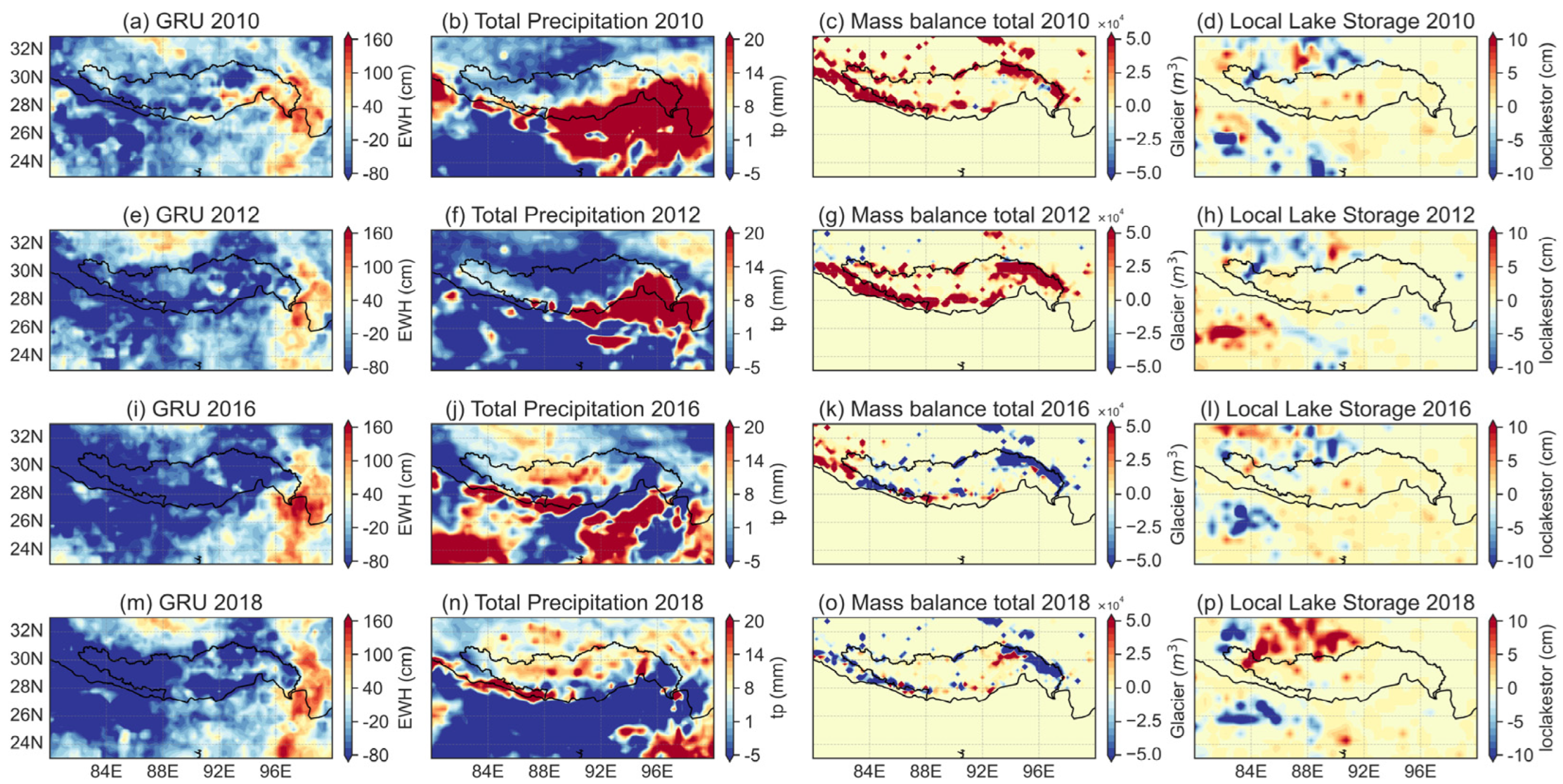
4.2. Representative Area-Brahmaputra Basin

To further investigate the high-resolution characteristics of the TWSA on the QTP and its discrepancies with other products in areas exhibiting notable differences, we selected a representative region, i.e., the Brahmaputra Basin, which is a highly mountain- and glacier-dominated region in the Himalayas. The comparison and analysis results of the other 11 sub-basins are detailed in the Supplementary Materials. Since the true resolution of mascon products ranges from 1° to 3°, their suitability for sub-basin comparisons is limited. In this case, we instead compared the GRU with GLWS2.0 (0.5°) in regions where it exhibited greater discrepancies from other models. As shown in Figure 10, the GRU model is capable of resolving hydrological features at the sub-basin scale, particularly in sensitive regions such as glacier-dense areas, active permafrost zones, and regions undergoing lake expansion, by capturing more pronounced spatiotemporal variability. Notable discrepancies are observed between the GRU model and GLWS2.0. The GRU model tends to capture stronger positive anomalies in the eastern region, whereas widespread negative EWH is evident in the central and western regions. In contrast, the GLWS2.0 model exhibits greater spatial heterogeneity. It is worth noting that the ability of the GRU model to capture complex multivariate nonlinear relationships is often regarded as a “black box”, and the model architecture and hyperparameters need to be repeatedly adjusted when applied to different regions or periods.
Additionally, we computed the annual mean values of EWH in conjunction with precipitation, glacier mass balance, and lake water levels (Figure 11). The results illustrate the spatiotemporal evolution of EWH within the Brahmaputra Basin, further elucidating the differences and consistencies between the GRU model and various reference datasets, including GLWS2.0, precipitation, glacier mass balance, and lake storage products. These analyses reveal that regions with high EWH variability often coincide with areas of elevated precipitation intensity, particularly during the monsoon months. However, in glacierized regions, precipitation alone does not fully explain the observed EWH. In other words, the contributions of meltwater and glacier mass balance are also significant.
Figure 12 compares changes over the period of 2002–2020 in the GRU versus GLWS2.0, the GRU versus the precipitation time series, the GRU versus glacier mass balance, and the GRU versus reservoir storage data. Both the GRU (orange line) and GLWS (blue line) time series exhibit a clear annual cycle, peaking during the monsoon season (approximately June to September) and declining during the pre-monsoon or winter months (approximately December to March). Notably, the GRU model displays sharper peaks and troughs, which may be attributed to the high-resolution downscaling capturing finer hydrological variations within small sub-basins. This finding is consistent with the discussions of Tapley et al. (2004) [61] and Landerer and Swenson (2012) [62], who noted that the GRACE is less effective at resolving small-scale basins.
Comparing the EWH obtained using the GRU with the precipitation (pink line) records, we can find a strong correlation between the timing of EWH increases and the onset of the monsoon: precipitation typically surges between June and September, driving infiltration, replenishing soil moisture, and recharging groundwater throughout most of the Brahmaputra Basin. Conversely, the negative EWH during the dry season aligns with minimal precipitation inputs. Mankin and Diffenbaugh (2015) have highlighted the dominant role of monsoon forcing in the Himalayan water budget [63]. The comparative analysis further reveals that the glacier signal (green line) appears superimposed on the broader EWH cycle and exhibits marked interannual variability. For example, in years with extensive melting, if meltwater is stored in downstream lakes or groundwater systems, a sudden EWH surge may occur, thereby influencing broader hydrological fluxes. Bolch et al. (2012) [64] and Yao et al. (2012) [7] have demonstrated that Himalayan glaciers retreat heterogeneously and exhibit complex mass balance trends, which may lead to intricate EWH responses. Note that the timing of maximum EWH often coincides with peak lake storage (yellow line); however, differences in magnitude suggest that certain subregions may experience more transient or pronounced lake expansions, potentially reflecting regulated reservoir operations or ephemeral glacier lakes.
Previous studies [65,66] have underscored the critical importance of downscaled GRACE or model data for elucidating subregional storage trends in complex terrains. Figure 13 further shows the EWH anomalies for the Brahmaputra Basin from 2003 to 2018. In 2003 and 2004, EWH values were relatively high, with positive anomalies reaching their maximum amplitude. Between 2005 and 2007, a series of moderate monsoon years and concomitant changes in glacier melt resulted in notable alterations in EWH. From 2008 to 2011, a transition to near-zero or slightly negative anomalies was observed, particularly from 2009 to 2010. This can be attributed to the interplay between evolving precipitation regimes and persistent glacier mass loss. Overall, water storage fluctuations in the Brahmaputra Basin are predominantly governed by seasonal cycles; storage typically peaks during the monsoon months before gradually declining during the winter dry season. This marked periodicity aligns well with previous analyses of Himalayan river systems [8,67]. In mountainous regions, EWH is influenced not only by precipitation but also by glacier mass balance. A negative glacier mass balance can trigger meltwater pulses that temporarily augment downstream water storage. However, once these waters are depleted, either exiting the basin system or being diverted for anthropogenic use, a long-term net negative EWH trend ensues.
Moreover, global warming, shifts in monsoon patterns, and the intensification of extreme events (floods and droughts) are expected to further modify EWH. The mechanistic explanation of how external factors, such as climate warming and monsoon variability, affect water storage remains insufficiently transparent, calling for validation through hydrological process models or simulation studies. Should global warming persist, Himalayan glaciers are likely to experience continued mass loss, which in turn will alter the seasonal characteristics of EWH at the Brahmaputra headwaters. The GRU downscaling approach has refined our understanding of EWH in the Brahmaputra Basin, with analyses indicating that terrestrial water storage is governed by the complex interplay of climatic factors, such as monsoon rainfall and glacier melt, and anthropogenic influences [59].

5. Conclusions

This study demonstrates a high-resolution, GRU-based framework for downscaling and gap-filling GRACE/GRACE-FO observations across the QTP. First, the deep learning approach significantly refines the spatiotemporal portrayal of the TWSA relative to coarse-resolution GRACE mascon solutions, thereby highlighting previously obscured hydrological signals in glacier-rich and rapidly changing permafrost regions. By leveraging multi-source datasets, including glacier mass balance, precipitation, snow cover, and evapotranspiration, the model captures the subtle interplay of climatic forcing, cryospheric processes, and water storage changes in sub-basins. Second, the GRU model provides a cohesive solution for bridging the data gaps in the GRACE and GRACE-FO missions. This temporal continuity is critical for monitoring long-term trends on the QTP, which is undergoing significant glacier retreat and lake expansion. Reconstructing missing data can provide important insights into the understanding and management of hydrological processes, such as how climate change and anthropogenic interventions affect water balance at the basin scales.
The application demonstrates both the strengths and weaknesses in the use of the GRU model for large-scale hydrological assessments. The GRU model’s capacity to learn nonlinear correlations among diverse input variables facilitates sharper estimates of the TWSA, but its dependence on consistent, high-quality input data may constrain performance in data-sparse environments. Similarly, the “black-box” nature of deep learning can limit the interpretability of results, particularly when isolating the effects of climate warming and monsoon variability on glacier-fed hydrological systems. Despite these shortcomings, the high-resolution, data-driven approach proposed here lays a foundation for more detailed representations of water storage across high-altitude plateaus. Future advances might incorporate hybrid modeling to merge deep learning with physical process representations or integrate emerging satellite missions for validation and assimilation.

Supplementary Materials

The following supporting information can be downloaded at: https://www.mdpi.com/article/10.3390/rs17081333/s1, Figures S1–S44: the GRU-derived TWSA of the 11 sub-basins (except for the Brahmaputra Basin, which is described in detail in the main text) in the Qinghai–Tibet Plateau and compares these results with the GLWS2.0 model.

Author Contributions

Conceptualization, J.C. and L.W.; methodology, J.C.; software, J.C. and Z.P.; validation, J.C., L.W. and C.C.; investigation, J.C. and L.W.; data curation, J.C. and Z.P.; writing—original draft, J.C.; writing—review and editing, L.W. and C.C.; funding acquisition, L.W. and C.C. All authors have read and agreed to the published version of the manuscript.

Funding

This research was funded by the National Natural Science Foundation of China (grant number 42274110 and 42374106).

Data Availability Statement

The Glacier PyGEM (0.1°, Monthly) can be accessed at https://nsidc.org/data/hma_gl_rcp/versions/1. Snow cover MODIS (0.005°, Daily) is available at https://data.tpdc.ac.cn/zh-hans/data/ (accessed on 4 March 2024). Soil moisture GLDAS (0.25°, Monthly) can be obtained from https://catalog.data.gov/dataset/. Groundwater WGHM (0.5°, Monthly) is accessible at https://doi.pangaea.de/10.1594/PANGAEA.948461. Lake water WGHM (0.5°, Monthly) can be accessed at https://doi.pangaea.de/10.1594/PANGAEA.948461. Precipitation ERA5 (0.25°, Monthly) is available at https://forum.ecmwf.int/. Evapotranspiration GLEAM (0.25°, Monthly) can be accessed at https://www.gleam.eu/. Temperature MODIS (0.25°, Monthly) is available at https://lpdaac.usgs.gov/products/mod11c3v006/. Streamflow CNRD (0.25°, Monthly) can be obtained from https://data.tpdc.ac.cn/. GRACE/GRACE-FO (CSR-SH, CSR-M, JPL-M, GSFC-M; 1~3°, Monthly) can be accessed at https://icgem.gfz-potsdam.de/sl/temporal, https://www2.csr.utexas.edu/grace/RL06_mascons.html, https://grace.jpl.nasa.gov/data/get-data/jpl_global_mascons/, and https://earth.gsfc.nasa.gov/geo/data/grace-mascons. GLWS GLWS2.0 (0.5, Monthly) is available at https://doi.pangaea.de/10.1594/PANGAEA.954742.

Acknowledgments

The authors would like to sincerely thank Jiajia Sun of the University of Houston for his insightful discussions and suggestions. This work greatly benefited from open-source resources, particularly the GRACE, PyGEM, GLEAM, GLDAS, WGHM, and GLWS2.0 datasets. The authors also express their deep appreciation for the developers and communities that maintain these resources.

Conflicts of Interest

The authors declare no conflicts of interest.

Abbreviations

GRACEGravity Recovery and Climate Experiment
GRACE-FOGravity Recovery and Climate Experiment and its Follow-On
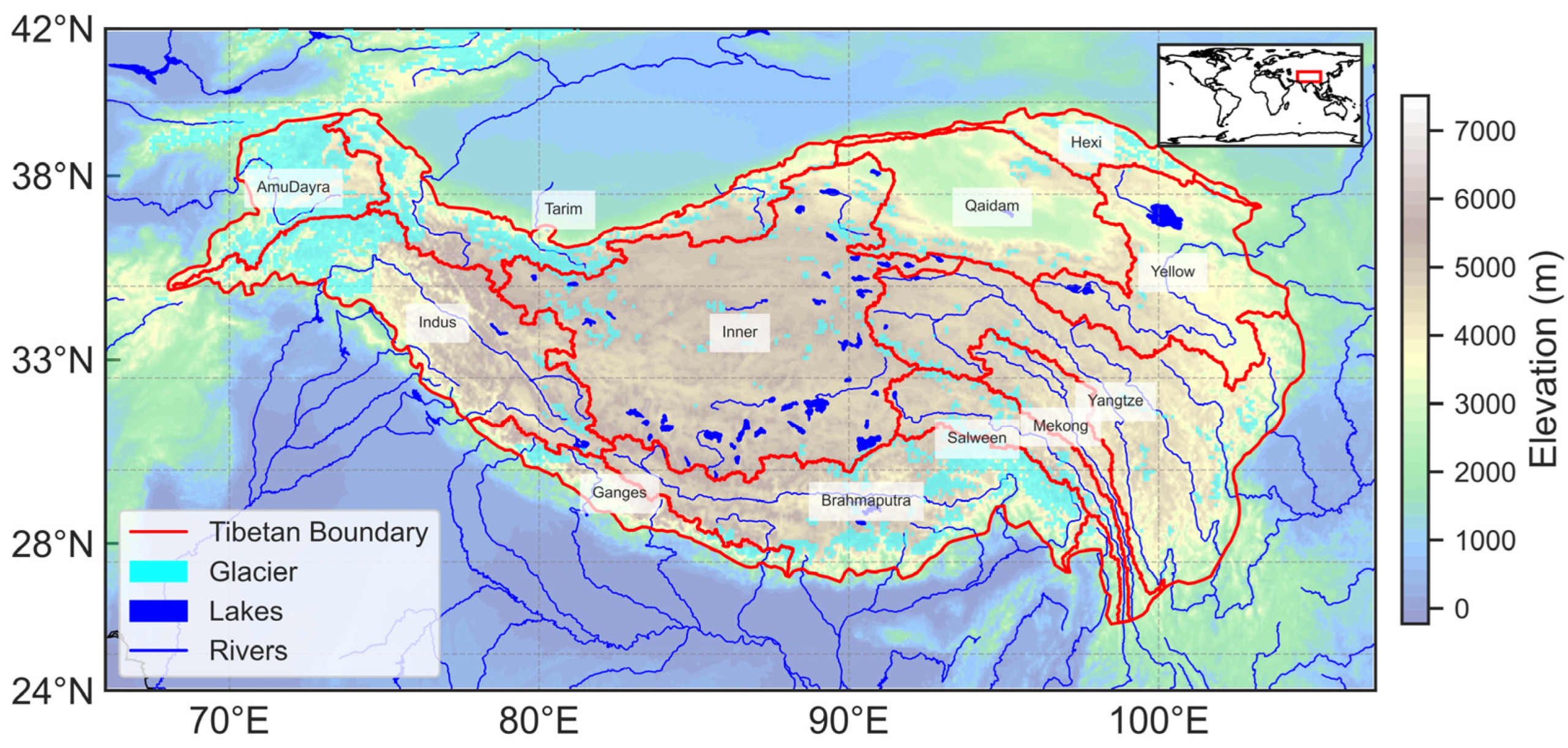
QTPQinghai–Tibet Plateau
CSRCenter for Space Research
JPLJet Propulsion Laboratory
GSFCGoddard Spaceflight Center
GLWS2.0Global Land Water Storage Dataset release 2
TWSATerrestrial Water Storage Anomalies
GLDASGlobal Land Data Assimilation System
WGHMWaterGAP Global Hydrology Model
PyGEMPython Glacier Evolution Model
ERA5European Centre for Medium-Range Weather Forecasts Reanalysis v5
MODISModerate Resolution Imaging Spectroradiometer
GLEAMGlobal Land Evaporation Amsterdam Model
CNRDChina Natural Runoff Dataset
GRUGated Recurrent Unit
MSEMean Squared Error
RMSERoot Mean Square Error
EWHEquivalent Water Height
CCCorrelation coefficient
NDVI Normalized Difference Vegetation Index

References

  1. Chen, T.; Pan, Y.; Ding, H.; Jiao, J.; He, M. Investigating Terrestrial Water Storage Variation and Its Response to Climate in Southeastern Tibetan Plateau Inferred through Space Geodetic Observations. J. Hydrol. 2024, 640, 131742. [Google Scholar] [CrossRef]
  2. Wang, G.; He, Y.; Huang, J.; Guan, X.; Wang, X.; Hu, H.; Wang, S.; Xie, Y. The Influence of Precipitation Phase Changes on the Recharge Process of Terrestrial Water Storage in the Cold Season over the Tibetan Plateau. J. Geophys. Res. Atmos. 2022, 127, e2021JD035824. [Google Scholar] [CrossRef]
  3. Wang, J.; Chen, X.; Hu, Q.; Liu, J. Responses of Terrestrial Water Storage to Climate Variation in the Tibetan Plateau. J. Hydrol. 2020, 584, 124652. [Google Scholar] [CrossRef]
  4. Beveridge, A.K.; Harig, C.; Simons, F.J. The Changing Mass of Glaciers on the Tibetan Plateau, 2002–2016, Using Time-Variable Gravity from the GRACE Satellite Mission. J. Geod. Sci. 2018, 8, 83–97. [Google Scholar] [CrossRef]
  5. Cheng, T.F.; Chen, D.; Wang, B.; Ou, T.; Lu, M. Human-Induced Warming Accelerates Local Evapotranspiration and Precipitation Recycling over the Tibetan Plateau. Commun. Earth Environ. 2024, 5, 388. [Google Scholar] [CrossRef]
  6. Lei, Y.; Li, R.; Letu, H.; Shi, J. Seasonal Variations of Recharge–Storage–Runoff Process over the Tibetan Plateau. J. Hydrometeorol. 2023, 24, 1619–1633. [Google Scholar] [CrossRef]
  7. Yao, T.; Thompson, L.; Yang, W.; Yu, W.; Gao, Y.; Guo, X.; Yang, X.; Duan, K.; Zhao, H.; Xu, B.; et al. Different Glacier Status with Atmospheric Circulations in Tibetan Plateau and Surroundings. Nat. Clim. Chang. 2012, 2, 663–667. [Google Scholar] [CrossRef]
  8. Immerzeel, W.W.; Van Beek, L.P.H.; Bierkens, M.F.P. Climate Change Will Affect the Asian Water Towers. Science 2010, 328, 1382–1385. [Google Scholar] [CrossRef] [PubMed]
  9. Pritchard, H.D. Asia’s Shrinking Glaciers Protect Large Populations from Drought Stress. Nature 2019, 569, 649–654. [Google Scholar] [CrossRef]
  10. Li, X.; Long, D.; Bridget, R.S.; Michael, E.M.; Li, X.; Tian, F.; Sun, Z.; Wang, G. Water Loss over the Tibetan Plateau Endangers Water Supply Security for Asian Populations. Nat. Clim. Chang. 2022, 12, 785–786. [Google Scholar]
  11. Tapley, B.D.; Watkins, M.M.; Flechtner, F.; Reigber, C.; Bettadpur, S.; Rodell, M.; Sasgen, I.; Famiglietti, J.S.; Landerer, F.W.; Chambers, D.P.; et al. Contributions of GRACE to Understanding Climate Change. Nat. Clim. Chang. 2019, 9, 358–369. [Google Scholar] [CrossRef] [PubMed]
  12. Xie, J.; Xu, Y.-P.; Yu, H.; Huang, Y.; Guo, Y. Monitoring the Extreme Flood Events in the Yangtze River Basin Based on GRACE and GRACE-FO Satellite Data. Hydrol. Earth Syst. Sci. 2022, 26, 5933–5954. [Google Scholar] [CrossRef]
  13. Zhang, G.; Bolch, T.; Chen, W.; Crétaux, J.-F. Comprehensive Estimation of Lake Volume Changes on the Tibetan Plateau during 1976–2019 and Basin-Wide Glacier Contribution. Sci. Total Environ. 2021, 772, 145463. [Google Scholar] [CrossRef] [PubMed]
  14. Meng, F.; Su, F.; Li, Y.; Tong, K. Changes in Terrestrial Water Storage During 2003–2014 and Possible Causes in Tibetan Plateau. J. Geophys. Res. Atmos. 2019, 124, 2909–2931. [Google Scholar] [CrossRef]
  15. Deng, H.; Pepin, N.C.; Liu, Q.; Chen, Y. Understanding the Spatial Differences in Terrestrial Water Storage Variations in the Tibetan Plateau from 2002 to 2016. Clim. Chang. 2018, 151, 379–393. [Google Scholar] [CrossRef]
  16. Tong, K.; Su, F.; Yang, D.; Hao, Z. Evaluation of Satellite Precipitation Retrievals and Their Potential Utilities in Hydrologic Modeling over the Tibetan Plateau. J. Hydrol. 2014, 519, 423–437. [Google Scholar] [CrossRef]
  17. Chen, W.; Liu, Y.; Zhang, G.; Yang, K.; Zhou, T.; Wang, J.; Shum, C.K. What Controls Lake Contraction and Then Expansion in Tibetan Plateau’s Endorheic Basin Over the Past Half Century? Geophys. Res. Lett. 2022, 49, e2022GL101200. [Google Scholar] [CrossRef]
  18. Iqbal, N.; Hossain, F.; Lee, H.; Akhter, G. Satellite Gravimetric Estimation of Groundwater Storage Variations Over Indus Basin in Pakistan. IEEE J. Sel. Top. Appl. Earth Obs. Remote Sens. 2016, 9, 3524–3534. [Google Scholar] [CrossRef]
  19. Mo, S.; Zhong, Y.; Forootan, E.; Mehrnegar, N.; Yin, X.; Wu, J.; Feng, W.; Shi, X. Bayesian Convolutional Neural Networks for Predicting the Terrestrial Water Storage Anomalies during GRACE and GRACE-FO Gap. J. Hydrol. 2022, 604, 127244. [Google Scholar] [CrossRef]
  20. Foroumandi, E.; Nourani, V.; Jeanne Huang, J.; Moradkhani, H. Drought Monitoring by Downscaling GRACE-Derived Terrestrial Water Storage Anomalies: A Deep Learning Approach. J. Hydrol. 2023, 616, 128838. [Google Scholar] [CrossRef]
  21. Lyu, Y.; Yong, B. A Novel Double Machine Learning Strategy for Producing High-Precision Multi-Source Merging Precipitation Estimates Over the Tibetan Plateau. Water Resour. Res. 2024, 60, e2023WR035643. [Google Scholar] [CrossRef]
  22. Yazdian, H.; Salmani-Dehaghi, N.; Alijanian, M. A Spatially Promoted SVM Model for GRACE Downscaling: Using Ground and Satellite-Based Datasets. J. Hydrol. 2023, 626, 130214. [Google Scholar] [CrossRef]
  23. Wang, Y.; Li, C.; Cui, Y.; Cui, Y.; Xu, Y.; Hora, T.; Zaveri, E.; Rodella, A.-S.; Bai, L.; Long, D. Spatial Downscaling of GRACE-Derived Groundwater Storage Changes across Diverse Climates and Human Interventions with Random Forests. J. Hydrol. 2024, 640, 131708. [Google Scholar] [CrossRef]
  24. Qian, N.; Gao, J.; Li, Z.; Yan, Z.; Feng, Y.; Yan, Z.; Yang, L. Bridging the Terrestrial Water Storage Anomalies between the GRACE/GRACE-FO Gap Using BEAST+GMDH Algorithm. Remote Sens. 2024, 16, 3693. [Google Scholar] [CrossRef]
  25. Yin, W.; Zhang, G.; Han, S.-C.; Yeo, I.-Y.; Zhang, M. Improving the Resolution of GRACE-Based Water Storage Estimates Based on Machine Learning Downscaling Schemes. J. Hydrol. 2022, 613, 128447. [Google Scholar] [CrossRef]
  26. Reichstein, M.; Camps-Valls, G.; Stevens, B.; Jung, M.; Denzler, J.; Carvalhais, N.; Prabhat, F. Deep Learning and Process Understanding for Data-Driven Earth System Science. Nature 2019, 566, 195–204. [Google Scholar] [CrossRef]
  27. Irrgang, C.; Saynisch-Wagner, J.; Dill, R.; Boergens, E.; Thomas, M. Self-Validating Deep Learning for Recovering Terrestrial Water Storage from Gravity and Altimetry Measurements. Geophys. Res. Lett. 2020, 47, e2020GL089258. [Google Scholar] [CrossRef]
  28. Tao, H.; Al-Sulttani, A.H.; Salih, S.Q.; Mohammed, M.K.A.; Khan, M.A.; Beyaztas, B.H.; Ali, M.; Elsayed, S.; Shahid, S.; Yaseen, Z.M. Development of High-Resolution Gridded Data for Water Availability Identification through GRACE Data Downscaling: Development of Machine Learning Models. Atmos. Res. 2023, 291, 106815. [Google Scholar] [CrossRef]
  29. Chung, J.; Gulcehre, C.; Cho, K.; Bengio, Y. Empirical Evaluation of Gated Recurrent Neural Networks on Sequence Modeling. arXiv 2014, arXiv:1412.3555. [Google Scholar]
  30. Yuan, D.-N. GRACE-FO. GRACEFO_L2_CSR_MONTHLY_0062. Ver. 6.2. PO.DAAC, CA, USA. (RL06.2). 2023. Available online: https://podaac.jpl.nasa.gov/dataset/GRACEFO_L2_CSR_MONTHLY_0062 (accessed on 4 March 2024).
  31. Hersbach, H.; Bell, B.; Berrisford, P.; Biavati, G.; Horányi, A.; Muñoz Sabater, J.; Nicolas, J.; Peubey, C.; Radu, R.; Rozum, I.; et al. ERA5 Hourly Data on Single Levels from 1940 to Present. Copernicus Climate Change Service (C3S) Climate Data Store (CDS). 2023. Available online: https://cds.climate.copernicus.eu/datasets/reanalysis-era5-single-levels?tab=documentation (accessed on 4 March 2024).
  32. Rounce, D.; Hock, R.; Maussion, F. Global PyGEM-OGGM Glacier Projections with RCP and SSP Scenarios. (HMA2_GGP, Version 1); NASA National Snow and Ice Data Center Distributed Active Archive Center: Boulder, Colorado, USA, 2022; Available online: https://nsidc.org/data/hma2_ggp/versions/1 (accessed on 4 March 2024).
  33. Pan, F.; Jiang, L.; Wang, G.; Pan, J.; Huang, J.; Zhang, C.; Cui, H.; Yang, J.; Zheng, Z.; Wu, S.; et al. MODIS Daily Cloud-Gap-Filled Fractional Snow Cover Dataset of the Asian Water Tower Region (2000–2022). Earth Syst. Sci. Data 2024, 16, 2501–2523. [Google Scholar] [CrossRef]
  34. Vermote, E.F.; Wolfe, R.E. MOD09GQ MODIS/Terra Surface Reflectance Daily L2G Global 250m SIN Grid V061; NASA EOSDIS Land Processes DAAC: Sioux Falls, SD, USA, 2021. Available online: https://lpdaac.usgs.gov/products/mod09gqv061/ (accessed on 4 March 2024).
  35. Martens, B.; Miralles, D.G.; Lievens, H.; Van Der Schalie, R.; De Jeu, R.A.M.; Fernández-Prieto, D.; Beck, H.E.; Dorigo, W.A.; Verhoest, N.E.C. GLEAM v3: Satellite-Based Land Evaporation and Root-Zone Soil Moisture. Geosci. Model Dev. 2017, 10, 1903–1925. [Google Scholar] [CrossRef]
  36. Gou, J.; Miao, C.; Duan, Q.; Tang, Q.; Di, Z.; Liao, W.; Wu, J.; Zhou, R. Sensitivity Analysis-based Automatic Parameter Calibration of the VIC Model for Streamflow Simulations over China. Water Resour. Res. 2020, 56, e2019WR025968. [Google Scholar] [CrossRef]
  37. Rodell, M.; Houser, P.R.; Jambor, U.; Gottschalck, J.; Mitchell, K.; Meng, C.-J.; Arsenault, K.; Cosgrove, B.; Radakovich, J.; Bosilovich, M.; et al. The Global Land Data Assimilation System. Bull. Am. Meteorol. Soc. 2004, 85, 381–394. [Google Scholar] [CrossRef]
  38. Müller Schmied, H.; Cáceres, D.; Eisner, S.; Flörke, M.; Herbert, C.; Niemann, C.; Peiris, T.A.; Popat, E.; Portmann, F.T.; Reinecke, R.; et al. The Global Water Resources and Use Model WaterGAP v2.2d: Model Description and Evaluation. Geosci. Model Dev. 2021, 14, 1037–1079. [Google Scholar] [CrossRef]
  39. Save, H.; Bettadpur, S.; Tapley, B.D. High-resolution CSR GRACE RL05 mascons. J. Geophys. Res. Solid Earth 2016, 121, 7547–7569. [Google Scholar] [CrossRef]
  40. Watkins, M.M.; Wiese, D.N.; Yuan, D.-N.; Boening, C.; Landerer, F.W. Improved Methods for Observing Earth’s Time Variable Mass Distribution with GRACE Using Spherical Cap Mascons. J. Geophys. Res. Solid Earth 2015, 120, 2648–2671. [Google Scholar] [CrossRef]
  41. Loomis, B.D.; Luthcke, S.B.; Sabaka, T.J. Regularization and Error Characterization of GRACE Mascons. J. Geod. 2019, 93, 1381–1398. [Google Scholar] [CrossRef]
  42. Gerdener, H.; Kusche, J.; Schulze, K.; Döll, P.; Klos, A. The Global Land Water Storage Data Set Release 2 (GLWS2.0) Derived via Assimilating GRACE and GRACE-FO Data into a Global Hydrological Model. J. Geod. 2023, 97, 73. [Google Scholar] [CrossRef]
  43. Tong, J.; Shi, Z.; Jiao, J.; Yang, B.; Tian, Z. Glacier Mass Balance and Its Impact on Land Water Storage in the Southeastern Tibetan Plateau Revealed by ICESat-2 and GRACE-FO. Remote Sens. 2024, 16, 1048. [Google Scholar] [CrossRef]
  44. Niranjannaik, M.; Kumar, A.; Beg, Z.; Singh, A.; Swarnkar, S.; Gaurav, K. Groundwater Variability in a Semi-Arid River Basin, Central India. Hydrology 2022, 9, 222. [Google Scholar] [CrossRef]
  45. Li, N.; Cuo, L.; Zhang, Y.; Flerchinger, G.N. Diurnal Soil Freeze-Thaw Cycles and the Factors Determining Their Changes in Warming Climate in the Upper Brahmaputra Basin of the Tibetan Plateau. J. Geophys. Res. Atmos. 2024, 129, e2023JD040369. [Google Scholar] [CrossRef]
  46. Wang, C.; Shi, H.; Hu, H.; Wang, Y.; Xi, B. Properties of Cloud and Precipitation over the Tibetan Plateau. Adv. Atmos. Sci. 2015, 32, 1504–1516. [Google Scholar] [CrossRef]
  47. Gao, G.; Zhao, J.; Wang, J.; Zhao, G.; Chen, J.; Li, Z. Spatiotemporal Variation and Driving Analysis of Groundwater in the Tibetan Plateau Based on GRACE Downscaling Data. Water 2022, 14, 3302. [Google Scholar] [CrossRef]
  48. Xiang, L.; Wang, H.; Steffen, H.; Jiang, L.; Shen, Q.; Jia, L.; Su, Z.; Wang, W.; Deng, F.; Qiao, B.; et al. Two Decades of Terrestrial Water Storage Changes in the Tibetan Plateau and Its Surroundings Revealed through GRACE/GRACE-FO. Remote Sens. 2023, 15, 3505. [Google Scholar] [CrossRef]
  49. Wang, Q.; Sun, Y.; Guan, Q.; Du, Q.; Zhang, Z.; Zhang, J.; Zhang, E. Exploring Future Trends of Precipitation and Runoff in Arid Regions under Different Scenarios Based on a Bias-Corrected CMIP6 Model. J. Hydrol. 2024, 630, 130666. [Google Scholar] [CrossRef]
  50. Xie, X.; He, B.; Guo, L.; Miao, C.; Zhang, Y. Detecting Hotspots of Interactions between Vegetation Greenness and Terrestrial Water Storage Using Satellite Observations. Remote Sens. Environ. 2019, 231, 111259. [Google Scholar] [CrossRef]
  51. Immerzeel, W.W.; Lutz, A.F.; Andrade, M.; Bahl, A.; Biemans, H.; Bolch, T.; Hyde, S.; Brumby, S.; Davies, B.J.; Elmore, A.C.; et al. Importance and Vulnerability of the World’s Water Towers. Nature 2020, 577, 364–369. [Google Scholar] [CrossRef]
  52. Pokhrel, Y.; Felfelani, F.; Satoh, Y.; Boulange, J.; Burek, P.; Gädeke, A.; Gerten, D.; Gosling, S.N.; Grillakis, M.; Gudmundsson, L.; et al. Global Terrestrial Water Storage and Drought Severity under Climate Change. Nat. Clim. Chang. 2021, 11, 226–233. [Google Scholar] [CrossRef]
  53. Long, D.; Pan, Y.; Zhou, J.; Chen, Y.; Hou, X.; Hong, Y.; Scanlon, B.R.; Longuevergne, L. Global Analysis of Spatiotemporal Variability in Merged Total Water Storage Changes Using Multiple GRACE Products and Global Hydrological Models. Remote Sens. Environ. 2017, 192, 198–216. [Google Scholar] [CrossRef]
  54. Yi, S.; Sneeuw, N. Filling the Data Gaps Within GRACE Missions Using Singular Spectrum Analysis. J. Geophys. Res. Solid Earth 2021, 126, e2020JB021227. [Google Scholar] [CrossRef]
  55. Zhang, X.; Li, J.; Dong, Q.; Wang, Z.; Zhang, H.; Liu, X. Bridging the Gap between GRACE and GRACE-FO Using a Hydrological Model. Sci. Total Environ. 2022, 822, 153659. [Google Scholar] [CrossRef]
  56. Haddeland, I.; Clark, D.B.; Franssen, W.; Ludwig, F.; Voß, F.; Arnell, N.W.; Bertrand, N.; Best, M.; Folwell, S.; Gerten, D.; et al. Multimodel Estimate of the Global Terrestrial Water Balance: Setup and First Results. J. Hydrometeorol. 2011, 12, 869–884. [Google Scholar] [CrossRef]
  57. Wang, Q.; Yi, S.; Sun, W. Continuous Estimates of Glacier Mass Balance in High Mountain Asia Based on ICESat-1,2 and GRACE/GRACE Follow-On Data. Geophys. Res. Lett. 2021, 48, e2020GL090954. [Google Scholar] [CrossRef]
  58. An, L.; Wang, J.; Huang, J.; Pokhrel, Y.; Hugonnet, R.; Wada, Y.; Cáceres, D.; Müller Schmied, H.; Song, C.; Berthier, E.; et al. Divergent Causes of Terrestrial Water Storage Decline Between Drylands and Humid Regions Globally. Geophys. Res. Lett. 2021, 48, e2021GL095035. [Google Scholar] [CrossRef]
  59. Brun, F.; Berthier, E.; Wagnon, P.; Kääb, A.; Treichler, D. A Spatially Resolved Estimate of High Mountain Asia Glacier Mass Balances from 2000 to 2016. Nat. Geosci. 2017, 10, 668–673. [Google Scholar] [CrossRef]
  60. Kääb, A.; Berthier, E.; Nuth, C.; Gardelle, J.; Arnaud, Y. Contrasting Patterns of Early Twenty-First-Century Glacier Mass Change in the Himalayas. Nature 2012, 488, 495–498. [Google Scholar] [CrossRef] [PubMed]
  61. Tapley, B.D.; Bettadpur, S.; Ries, J.C.; Thompson, P.F.; Watkins, M.M. GRACE Measurements of Mass Variability in the Earth System. Science 2004, 305, 503–505. [Google Scholar] [CrossRef]
  62. Landerer, F.W.; Swenson, S.C. Accuracy of Scaled GRACE Terrestrial Water Storage Estimates. Water Resour. Res. 2012, 48, 2011WR011453. [Google Scholar] [CrossRef]
  63. Mankin, J.S.; Diffenbaugh, N.S. Influence of Temperature and Precipitation Variability on Near-Term Snow Trends. Clim. Dyn. 2015, 45, 1099–1116. [Google Scholar] [CrossRef]
  64. Bolch, T.; Kulkarni, A.; Kääb, A.; Huggel, C.; Paul, F.; Cogley, J.G.; Frey, H.; Kargel, J.S.; Fujita, K.; Scheel, M.; et al. The State and Fate of Himalayan Glaciers. Science 2012, 336, 310–314. [Google Scholar] [CrossRef]
  65. Girotto, M.; De Lannoy, G.J.M.; Reichle, R.H.; Rodell, M. Assimilation of Gridded Terrestrial Water Storage Observations from GRACE into a Land Surface Model: Grace Assimilation into a Land Surface Model. Water Resour. Res. 2016, 52, 4164–4183. [Google Scholar] [CrossRef]
  66. Long, D.; Scanlon, B.R.; Longuevergne, L.; Sun, A.Y.; Fernando, D.N.; Save, H. GRACE Satellite Monitoring of Large Depletion in Water Storage in Response to the 2011 Drought in Texas. Geophys. Res. Lett. 2013, 40, 3395–3401. [Google Scholar] [CrossRef]
  67. Bookhagen, B.; Burbank, D.W. Toward a Complete Himalayan Hydrological Budget: Spatiotemporal Distribution of Snowmelt and Rainfall and Their Impact on River Discharge. J. Geophys. Res. Earth Surf. 2010, 115, F3. [Google Scholar] [CrossRef]
Figure 1. Overview of geographical and hydrological components of the Qinghai–Tibet Plateau (QTP) and its 12 sub-basins. Red lines delineate the boundaries of the sub-basin. The base map depicts elevation, with light indicating glacier locations and blue representing lakes and rivers. The study area is located in the red box on the world map in the upper right corner.
Remotesensing 17 01333 g001
Figure 2. Flowchart of the study design and research structure, divided into four parts: data introduction, processing, modeling development and prediction, and downscaling result.
Remotesensing 17 01333 g002
Figure 3. Evaluation during model training. (a) Comparison between actual and predicted values. (b) The distribution of true and predicted values. (c) Training loss curve showing the changes in loss values during the model training process.
Remotesensing 17 01333 g003
Figure 4. Comparison of EWH seasonal, interannual, and long-term trends between three mascon models (CSR, JPL, and GSFC) and GRU predictions. (ad) illustrates the seasonal amplitude in EWH. (eh) displays the interannual component. (il) depicts the long-term EWH trend. (mp) presents the average annual EWH for 2010.
Remotesensing 17 01333 g004
Figure 5. The EWH time series of the entire QTP from 2003 to 2018. (a) Comparison of the GRU output with mascon results. Shading indicates periods with missing data. (b) Annual GRU-based EWH estimates for the entire region. (c) Seasonal cycles predicted by the GRU model and mascon results. (d) Comparison of spatial spectra between the GRU and the mascon solutions.
Remotesensing 17 01333 g005
Figure 6. The EWH time series of 12 sub-basins ((al) correspond to AmuDayra, Brahmaputra, Ganges, Hexi, Inner, Qaidam, Mekong, Indus, Salween, Tarim, Yangtze and Yellow, respectively) on the QTP estimated by the GRU model.
Remotesensing 17 01333 g006
Figure 7. Comparison between the GLWS2.0 model and the GRU-derived results during several gaps in the GRACE data. (a,c,e,g,i,k) represents the GLWS results. (b,d,f,h,j,l) represents the GRU results.
Remotesensing 17 01333 g007
Figure 8. Analysis of the differences between the GRU EWH and three mascon models (JPL, CSR, and GSFC mascon).
Remotesensing 17 01333 g008
Figure 9. The RMSE of the GRU model and the GLWS2.0 model with the original GRACE SH solution in distribution and time series, respectively. (a) The RMSE spatial distribution between the GRU and original GRACE SH solution. (b) The RMSE spatial distribution between the GLWS2.0 and original GRACE SH solution. (c) The time series of RMSE for each month in the QTP (the black circled area).
Remotesensing 17 01333 g009
Figure 10. Comparison of GRU model (a,c,e,g) and GLWS2.0 model (b,d,f,h) for the Brahmaputra Basin in 2010, 2012, 2016, and 2018, respectively.
Remotesensing 17 01333 g010
Figure 11. Comparing the GRU EWH (a,e,i,m) with the annual averages of total precipitation (b,f,j,n), glacier mass balance total (c,g,k,o), and local lake storage (d,h,l,p) for the Brahmaputra Basin in 2010, 2012, 2016, and 2018, respectively.
Remotesensing 17 01333 g011
Figure 12. Comparison of the average time series of GRU and GLWS EWH with precipitation, total glacier mass balance, and lake water in the Brahmaputra Basin.
Remotesensing 17 01333 g012
Figure 13. The EWH time series statistical results of the Brahmaputra Basin. The color change represents the change in time, from blue to red representing from 2003 to 2018.
Remotesensing 17 01333 g013
Table 1. Data used for GRU downscaling and model validation.
Data ItemSolutionsResolutionTime RangeData Source (DOI)
SpatialTemporal
Glacier mass balancePyGEM0.1°MonthlyJanuary 2000–December 210010.5067/H118TCMSUH3Q
Snow coverMODIS0.005°DailyFebruary 2000–Present10.11888/Cryos.tpdc.272503
Soil moistureGLDAS0.25°MonthlyJanuary 1948–Present10.5067/SXAVCZFAQLNO
Groundwater storageWGHM0.5°MonthlyJanuary 1902–December 201910.1594/PANGAEA.948461
Lake water storageWGHM0.5°MonthlyJanuary 1902–December 201910.1594/PANGAEA.948461
PrecipitationERA50.25°MonthlyJanuary 1940–Present10.24381/cds.f17050d7
EvapotranspirationGLEAM0.25°MonthlyJanuary 2003–December 202210.5194/gmd-10-1903-2017
TemperatureMODIS0.25°MonthlyMarch 2000–Present10.5067/MODIS/MOD11C3.006
StreamflowCNRD0.25°MonthlyJanuary 1961–December 201810.11888/Atmos.tpdc.272864
TWSACSR-SH #
CSR-M *
JPL-M
GSFC-M
1~3°MonthlyApril 2002–Present10.5067/GRGSM-20C06
10.18738/T8/UN91VR
10.5067/TEMSC-3JC634
10.1007/s00190-019-01252-y
TWSGLWS2.00.5MonthlyJanuary 2003–December 201910.1594/PANGAEA.954742
#: SH represents the spherical harmonic solution. *: M represents the mascon solution.
Disclaimer/Publisher’s Note: The statements, opinions and data contained in all publications are solely those of the individual author(s) and contributor(s) and not of MDPI and/or the editor(s). MDPI and/or the editor(s) disclaim responsibility for any injury to people or property resulting from any ideas, methods, instructions or products referred to in the content.

