Historical Coast Snaps: Using Centennial Imagery to Track Shoreline Change

Abstract

Understanding long-term coastal evolution requires historical data, yet accessing reliable information becomes increasingly challenging for extended periods. While vertical aerial imagery has been extensively used in coastal studies since the mid-20th century, and satellite-derived shoreline measurements are now revolutionizing shoreline change studies, ground-based images, such as historical photographs and picture postcards, provide an alternative source of shoreline data for earlier periods when other datasets are scarce. Despite their frequent use for documenting qualitative morphological changes, these valuable historical data sources have rarely supported quantitative assessments of coastal evolution. This study demonstrates the potential of historical ground-oblique images for quantitatively assessing shoreline position and long-term change. Using Conceição-Duquesa Beach (Cascais, Portugal) as a case study, we analyze shoreline evolution over 92 years by applying a novel methodology to historical photographs and postcards. The approach combines image registration, shoreline detection, coordinate transformation, and rectification while accounting for positional uncertainty. Results reveal a significant counterclockwise rotation of the shoreline between the 20th and 21st centuries, exceeding estimated uncertainty thresholds. This study highlights the feasibility of using historical ground-based imagery to reconstruct shoreline positions and quantify long-term coastal change. The methodology is straightforward, adaptable, and offers a promising avenue for extending the temporal range of shoreline datasets, advancing our understanding of coastal evolution.

1. Introduction

Coastal evolution studies play a pivotal role in understanding the dynamics of coastal regions and evaluating the potential impacts of climate change and human activities on these environments. Quantitative shoreline changes studies remain as one of the most widely used methods to analyze beach and nearshore morphodynamic trends based on changes in coastal position [1]. This approach provides invaluable insights into how the coastal system is evolving over time [2,3,4,5,6,7], including the evolution at decadal to centennial scales [1,8], and it is now being revolutionized by the use of satellite-derived shorelines to analyze very recent morphodynamic change [9,10,11]. But the lack of centennial datasets remains a significant challenge in longer-term historical shoreline change analysis [3,12,13].

To assess shoreline position changes at multidecadal to centennial scales, studies resort to historical data, despite the larger uncertainty associated with the older datasets [14]. Quantifying these errors enables the assessment of their magnitude relative to the studied signal. If the uncertainty is smaller than the signal, the results can be considered trustworthy.

Multidecadal shoreline evolution studies, spanning the 20th century, frequently use satellite and aerial photography, with the first potentially covering the last two to three decades and the air photographs extending back to the mid-century (in most cases) [1]. The scarcity of older datasets, and the difficulty in identifying and using shoreline indicators on such records [15,16], makes the task of assessing shoreline change at longer timescales challenging.

Ground-based images of the beach system are available from much earlier, allowing the analysis to be extended into the late 19th century [17], but few studies have used this type of dataset to support quantitative analyses [18,19]. These types of images can be used to extend the period of shoreline analysis [20], but the development of tailored methods can help to mitigate the inherent effect of using older images, where less fundamental information is available.

The research presented here originates from a desire to make use of the information depicted on historical ground-based photographs and postcards about the morphological state of the coast. The aim is to use a rich dataset of old imagery in a quantifiable procedure, thereby extending the time available for shoreline change analyses. A novel approach to assess shoreline change and evolution is presented here, using archival ground-based photographs of a beach, alongside traditional and emerging remote-sensing datasets to determine shoreline positions (the latter used in this work for validation purposes). As a case study, the research focuses on a shore-platform sandy beach situated in Cascais, Portugal—a destination for tourists and photographers alike. The use of historical picture postcards represents an unconventional yet useful data source for our objectives. Coupled with existing approaches, this method can help extend the temporal scope of shoreline change analysis in this type of shore. The proposed methodology can be implemented elsewhere, with a few practical adjustments.

2. Study Area

The developed approach was applied and tested at Conceição-Duquesa urban beach, located at Cascais Riviera, Portugal (Figure 1). Situated along the central-western coast of Portugal, the Cascais Riviera has been a tourist destination since the 19th century. Renowned for its beautiful beaches, rich cultural heritage, mild climate, and proximity to the country’s capital [16,21,22], Cascais is well represented in the photographic record, including most of its sandy beaches [23].

Conceição-Duquesa beach, located in the southern sector of the Cascais shoreline, is sheltered by Cape Raso from the dominant high-energy north-westerly Atlantic wave swells (Figure 1) [16]. The nearshore wave climate within the embayment was assessed at a depth of 10 m using the simulation procedure described in [24]. The results show that this sheltering effect significantly influences the nearshore wave regime by substantially reducing incident wave energy and modulating the directional distribution of waves, which is characterized by a single dominant wave direction [24]. The simulation point, represented by a yellow dot in Figure 1, indicates an average significant wave height of 0.72 m, a mean wave period of 10.5 s, and a mean wave direction of 210° [24]. Tides are semidiurnal and mesotidal with mean tidal ranging from 1.15 m to 3.26 m, low to high tide, respectively [22].

The southern sector of Cascais coast presents a rocky shore with closed embayed beaches, like Conceição-Duquesa (CD), with potential littoral drift directed to the east [16]. CD beach is a shore platform sandy beach with artificial structures at the back and east limits, and a rocky outcrop in the western limit [16]. Beach length is approximately 300 m, oriented NE-SW, with a width ranging from around 50 m on the east-northeast side to approximately 80 m on the west-southwest part, filled with beach sand of medium-sand grain size [22]. The present-day characteristic beach profile exhibits a berm height located at 3.7 m MSL (mean sea level) and a beach face slope of 0.08 (modal values, [16]). The timelapse of Conceição-Duquesa (CD) beach [25]—a set of beach photographs acquired at CD beach using mobile phones, between February and October 2019, reveals a stable beach with small cross-shore seasonal variability. These results are in agreement with previous works showing intra- and inter-annual stability of Cascais embayment beaches [16,26]. The Conceição-Duquesa timelapse was created using the images acquired in the framework of a community beach monitoring program for Cascais beaches—CoastSnap Cascais (CSC) project—which implemented 17 fixed points (monitoring stations) on different Cascais beaches, allowing the monitoring of beach behavior by acquiring photographs at the same position of a particular beach [27]; CSC is part of the worldwide citizen science CoastSnap project [28].

Figure 1. Location of the study area, Conceição-Duquesa (CD) beach, in Cascais, central-west coast of continental Portugal. Red pin indicates the CoastSnap Cascais Station position, from which the photographs were used. Yellow dot (bottom right image) indicates the location of the simulation point used in the wave propagation model for Cascais bay [24]. The marina location is also indicated. Black letters in the base image indicate some buildings used as landmarks in the registration process: Loulé (LM), Lancastre (LtM) and Faial (FM) Manors [23]. Gray shaded areas in the main image, are not visible from the photograph point of view in CD beach. Base image: 2018 national ortho photographic coverage [29] and ArcGIS Pro^® basemaps.

Figure 1. Location of the study area, Conceição-Duquesa (CD) beach, in Cascais, central-west coast of continental Portugal. Red pin indicates the CoastSnap Cascais Station position, from which the photographs were used. Yellow dot (bottom right image) indicates the location of the simulation point used in the wave propagation model for Cascais bay [24]. The marina location is also indicated. Black letters in the base image indicate some buildings used as landmarks in the registration process: Loulé (LM), Lancastre (LtM) and Faial (FM) Manors [23]. Gray shaded areas in the main image, are not visible from the photograph point of view in CD beach. Base image: 2018 national ortho photographic coverage [29] and ArcGIS Pro^® basemaps.

This beach was chosen because of the availability of data on present morphological configuration (topographic and shoreline position) (Figure 1) and historical picture postcards depicting the beach configuration (Figure 2).

3. Materials and Methods

3.1. Datasets

3.1.1. Present-Day Beach Image

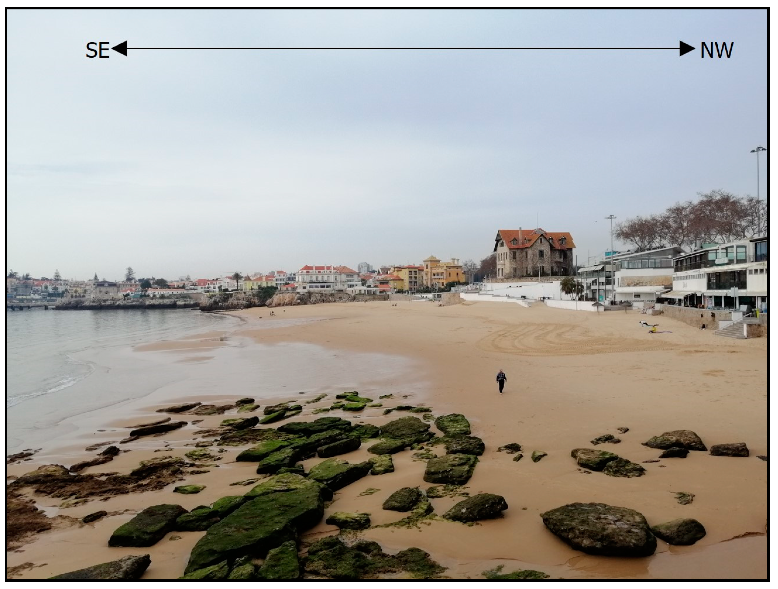
Present-day images of Conceição-Duquesa (CD) beach (Figure 3) were taken at a static point, CD CoastSnap Cascais station (Figure 1), during the field survey, at 11:03 a.m., on 3 February 2022 (winter season), at low tide. One of the images was used for the present-day reference and the master in the image processing procedures.

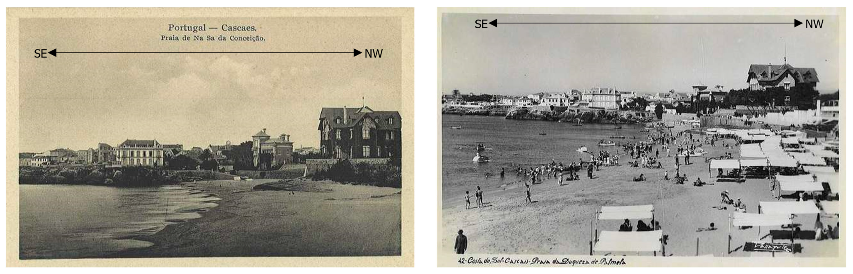
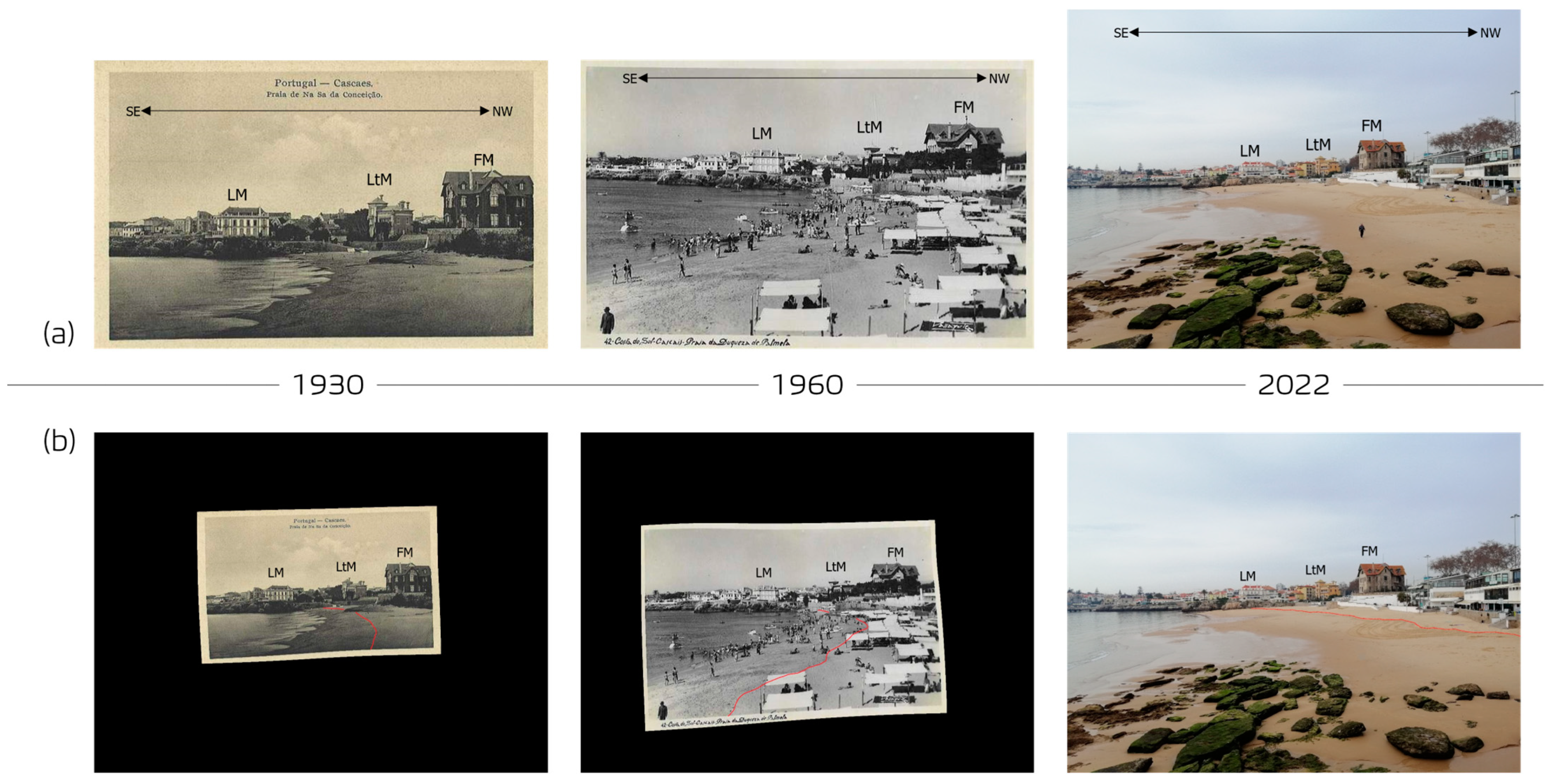
3.1.2. Historical Beach Images

Several historical images, such as picture postcards and old, historical photographs, offer glimpses of Conceição-Duquesa beach through varying perspectives. CoastSnap Cascais, the citizen–science project with stations for photograph acquisitions of beaches across Cascais municipality [27], provided the contemporary framework for selecting two old images that best matched the current scenes. The historical datasets consist of two picture postcards (Figure 2), one from 1930 [17] and another from 1960 [23]. The exact date when the images were taken is unknown, but the year is indicated for each postcard and is coherent with ancient landmarks and other historical references.

Regarding the season, the 1960 image is assumed to be of summertime, due to the presence of summer stalls (typically placed in the beginning of the summer and removed at the end) and because bathers are wearing swimming suits and trunks. In the 1930 photograph, it was assumed to be outside of the summer season because there were no stalls present and no people on the beach.

The rocky headland, at the SW limit of the beach, can be used as reference to estimate the tide level depicted in the older images, as the different rocky horizontal layers can be easily recognized in the images. In the 1930 image, the instantaneous water line (IWL) is consistent with a low-tide level, as observed in several other sources ([23] and CoastSnap Cascais project photographs [27]). In the 1960 image, IWL aligns a bit higher than the older image, but the beach width is still wide, and the bathers are concentrated near the water line and far from the stalls. This fact also favors the notion of a low-tide water level; and high-tides are depicted in other photographs [23] as almost touching the summer stalls. As such, we are confident that both historical images (Figure 3) present a water level near the low tide, and where the high-water line is clearly visible. Considering that Conceição-Duquesa beach has a relatively stable beach profile all year round (refer to Section 2), seasonal variations were assumed as less important and disregarded for the purpose of this study.

3.2. Reference Case

The reference case represents the present-day beach morphology and includes the necessary procedures to collect key data that assures the consistency of image processing and validation steps.

For this purpose, a field survey was conducted at Conceição-Duquesa beach, on the 3 February 2022, that consisted of the following:

(1)

A topographic survey, with real-time kinematic–differential global positioning system, covering the beach area, which also included the survey of 19 ground control points (GCP), evenly spread along the sub-aerial beach.

(2)

A total of 19 oblique photographs were taken at the CoastSnap Cascais (CSC) station, ensuring a static image acquisition, each one depicting the precise location, on the beach and on the image, of each GCP position. The approach took advantage of the existence of a CSC station, allowing photographs of the beach to be taken with the same field of view. Ensuring the static process of the image acquisition procedure is paramount for the image processing phase; in the absence of a CoastSnap station, static image acquisition can also be achieved using a camera tripod.

(3)

An unmanned aerial vehicle survey was performed to generate a digital elevation model and an orthomosaic of the sub-aerial beach, in support of the calibration and validation procedures.

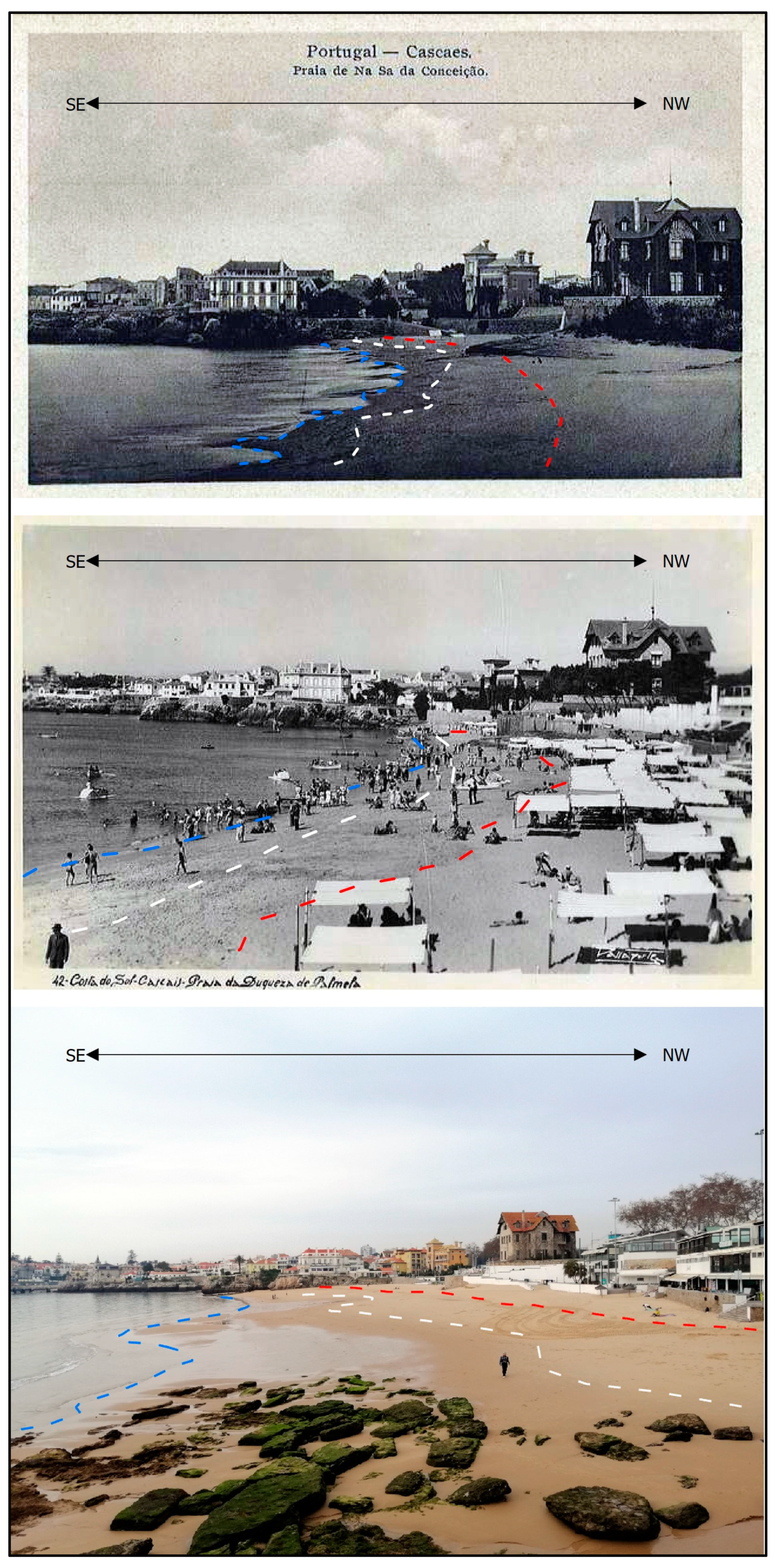
3.3. Shoreline Indicator

Shoreline change studies must rely on an indicator that can be simultaneously identifiable in all datasets and be less impacted by short-term variations [15,16]. According to [30], different shoreline position indicators can be used based on the proxy and method of collection (e.g., morphology-based, imagery-based, and elevation-based).

Analyzing all available photographs, several common shoreline position indicators could be recognized as suitable (Figure 4 and Figure 5): instantaneous water line [15], wet–dry line [30], and high-tide swash line (HTSL) [24]. All indicators are influenced by short-term variations, albeit to varying degrees. The high-water level (HWL) is one of the most used shoreline position indicators and the least affected by short-term variations [15], thus it was considered suitable for the analysis. To recognize the HWL position on the images, this study adopted the HTSL as a proxy as suggested by [30].

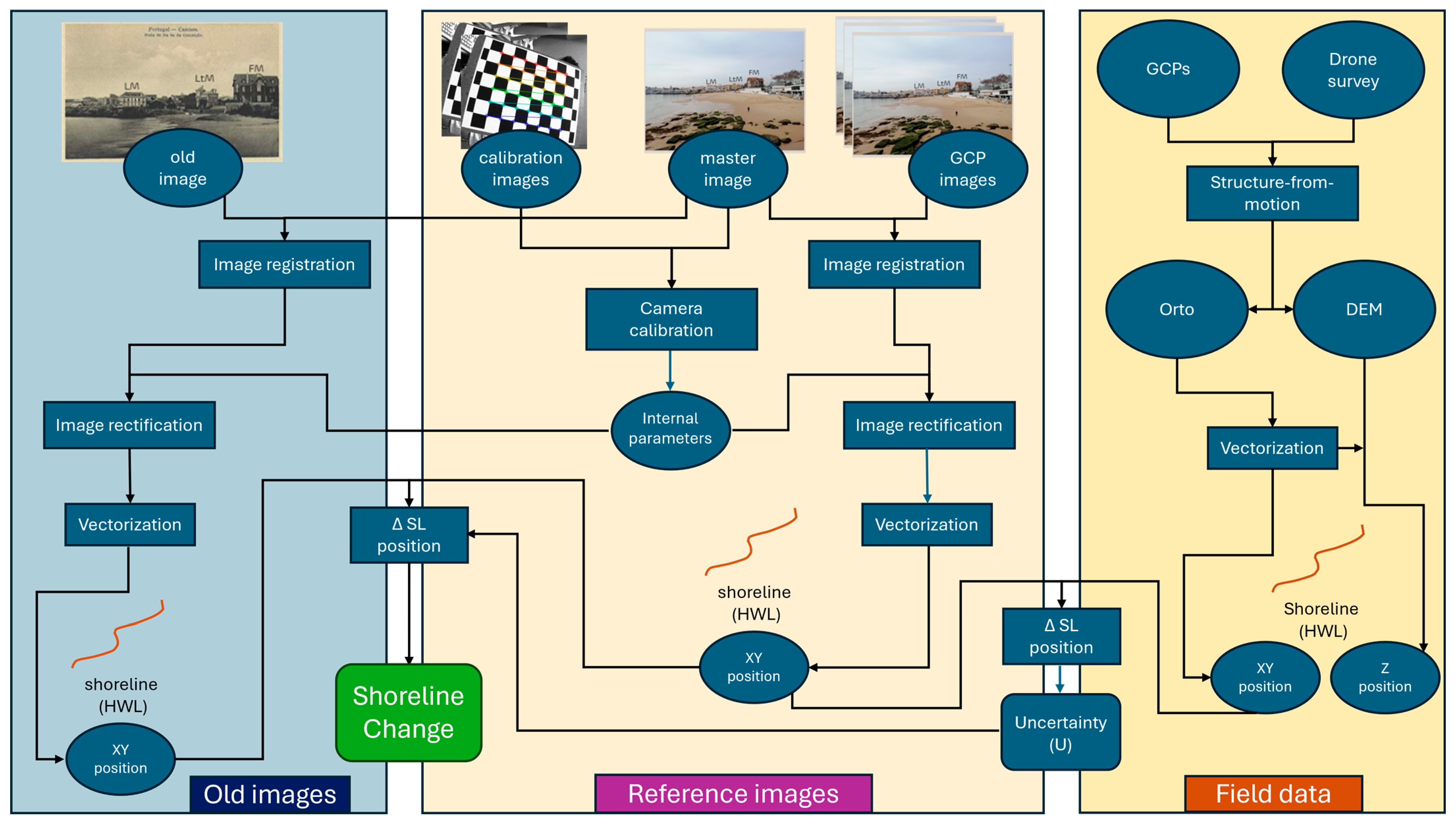
3.4. Image Processing

The image processing stage comprises three consecutive procedures: registration, shoreline detection/vectorization, and rectification. Figure 6 presents a graphical representation of the workflow.

3.4.1. Image Registration

The registration process coaligns different images by finding a transformation between the transformed target images and the reference image [31]. This process was performed in two separate ways, depending on the type of dataset used.

For the present-day, 19 images of ground control points position and the master image, acquired at the static CoastSnap Cascais station, registration process was carried out using the auto-align function of Adobe Photoshop^® software (https://www.adobe.com/products/photoshop.html, accessed on 13 January 2025).

Because the intrinsic camera parameters (ICP) of older photographs cannot be determined in advance, this study presents an approach that enables the use of old images without requiring prior knowledge of their ICP. The registration procedure between historical and present-day photographs enables the use of the estimated intrinsic camera parameters obtained through the calibration of the reference images (Section 3.4.3). This approach treats the intrinsic parameters as constants during the rectification process, ensuring consistency and accuracy. The auto-aligned procedure used for the present-day images was not capable of automatically aligning the older images with the master one, due to large differences between the two. Instead, we used the georeferencing capability of GIS software (ArcGIS Pro^® version 3.4.0) to mimic the registration process, where common elements were identified on the target images (old images) and matching the master one (2022 image). Some buildings were also used as landmarks, namely, the Loulé Manor (LM), the Lancastre Manor (LtM) and the Faial Manor (FM) [23] (Figure 1 and Figure 7). The registration step selected 17 and 22 common elements, respectively, for the 1930 and 1960 images (Figure 7), and the spline transformation method was used to align the old images to the 2022 master (Figure 7 and Figure 8b). Different transformation methods were tested, and the spline method provided the best results.

The proposed manual co-registration procedure is regarded as essential when working with older datasets, where there is no prior knowledge of the camera intrinsic camera parameters and usually fewer common elements to align the images.

3.4.2. Shoreline Highlighting

The highlight of the shoreline position on the original images was performed by drawing a red line [32] on the images using Windows Paint© photograph editing software v. 22H2 (refer to Figure 8b). This procedure is essential because the rectification process distorts the image pixels (see Figure on Section 3.4.3), making it difficult to identify the shoreline position on the rectified image. This is especially true for the older images (usually in a gray scale and with lower pixel resolution). This additional procedure facilitates shoreline detection and vectorization on the rectified images.

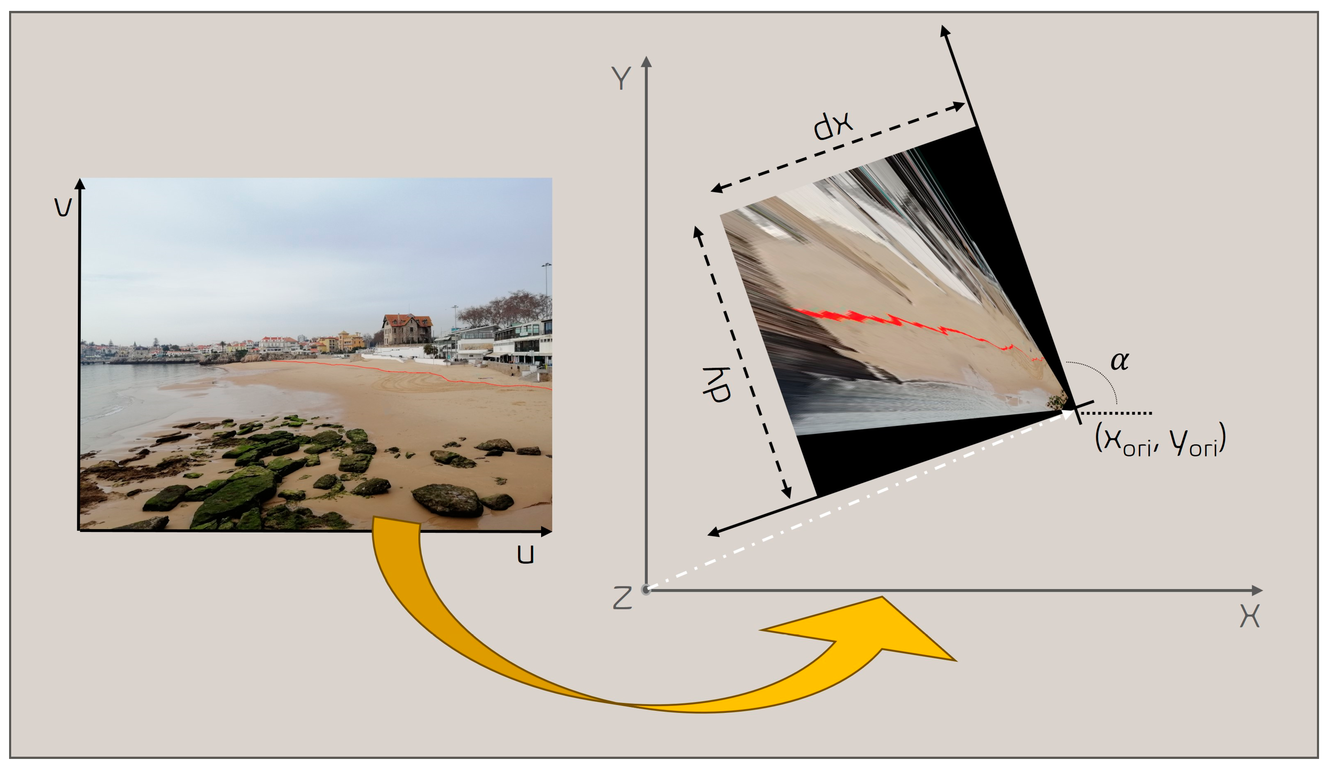
3.4.3. Image Rectification

The rectification process transforms the image pixel coordinates (u,v) into world metric coordinates (X,Y). This procedure uses ground control points (GCP) with known pixel locations on the target image (Figure 9), the position of the image acquisition, camera parameters, and a reference plan of rectification (Z_plane) (Figure 10). For further details on the method, please refer to [28,33,34]. Because the rectification process is affected by relief displacement, only image pixels located at the chosen elevation reference plane are correctly placed [35].

Camera internal parameters (focal length, position of the principal point, pixel skew and distortion coefficients) for the 2022 smartphone images with a resolution of 5120 × 3840 were estimated using the calibration process described in [33]. Image distortions induced by camera optics were estimated using opencv camera calibration algorithm [36] and based on Zhang’s method [31], which accounts for both tangential and radial distortion components. Eighteen photographs of a calibrated checkboard pattern with 11 columns and 8 rows were taken from different views, using the same smartphone used in the field survey to acquire the present-day calibration photographs (ground control points and master images). The approach was used with default parametrization described in [36] and yielded a total error of 0.199 pixels, allowing us to estimate the intrinsic parameters needed for image correction. The intrinsic camera parameters estimated were used in the rectification process of COSMOS code and described in the camera file input dataset.

The transformation procedure used the COSMOS algorithm [33] in python language, which is freely available at https://github.com/RuiTaborda/COSMOS (accessed on 13 January 2025). The code was developed to use a local coordinate system (allowing the x axis to be sub-parallel to the shoreline) that forms an arbitrary angle with the real-world coordinate system (α in Figure 10), aligning the shoreline main direction with the axis direction, where pixel distortion is minimized. 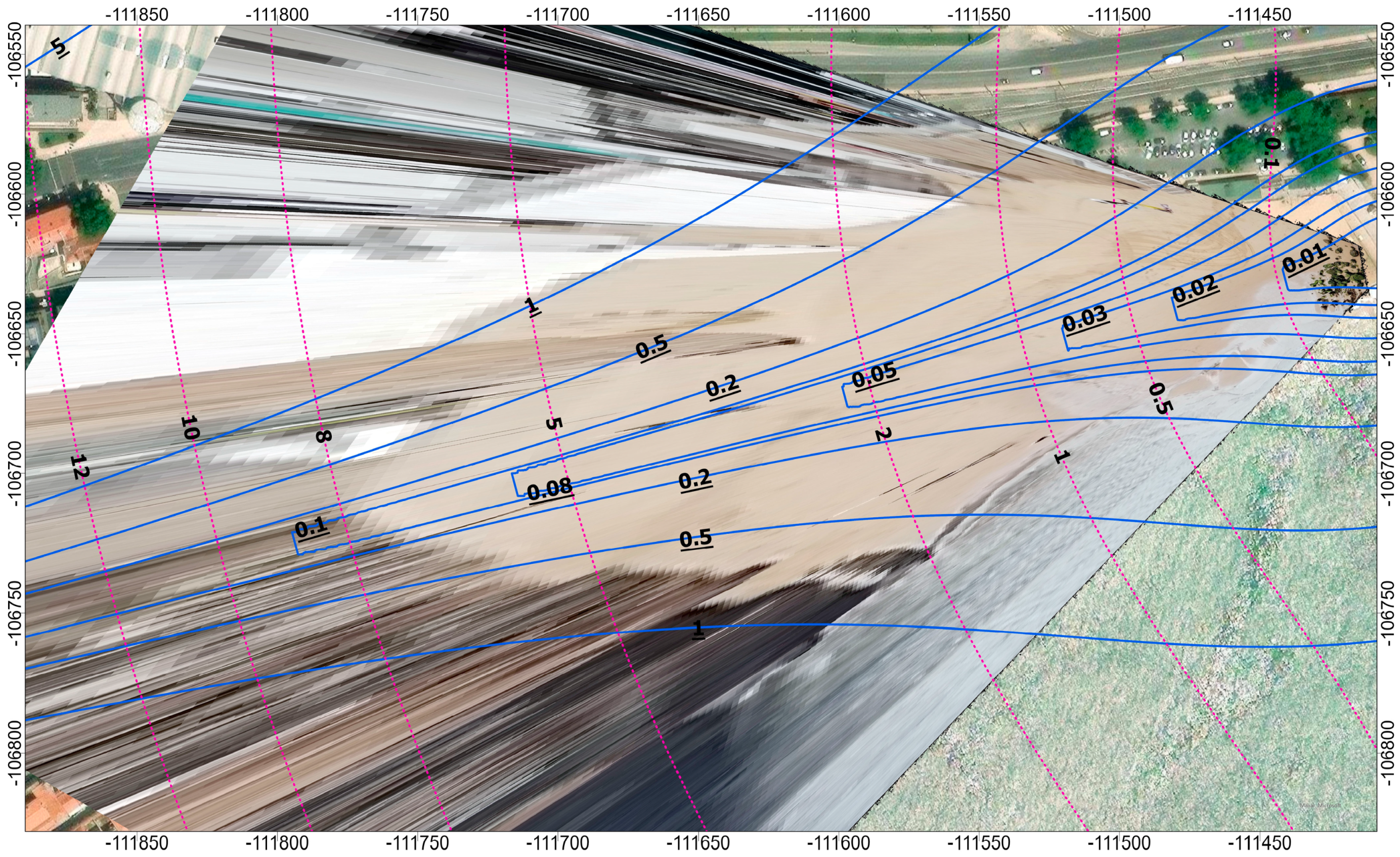Figure 11 shows the pixel footprint in meters in the longshore and cross-shore directions, demonstrating the efficacy of the procedure mentioned earlier. Furthermore, after the rectification process is complete, the code writes a Tiff World file (plain text file with the six parameters used in the affine transformation from image coordinates into map coordinates), allowing the resulting rectified georeferenced images to be directly imported into standard GIS applications [33].

Estimation of High-Water Line Elevation—Z_Plane

As the objective of this work is to assess the shoreline cross-shore positional variations, the reference plane used in the rectification process (Z_plane) must match the shoreline height identified on each image—in this case the high-water line (HWL).

To estimate the HWL elevation (Z-plane height), this study assumed that the beach can be described by an equilibrium average profile [37] and that no significant natural changes to the wave regime of the study area have occurred.

Similar to other works (e.g., [15,30,38]), the HWL can be expressed by a datum-based elevation, the mean high water (MHW) (Figure 4). For the present work, the MHW was considered to be represented by the annual average of maximum high-tide relative to mean sea level (MSL)—vertical reference system Cascais Helmert 38, estimated for each image year: 1930, 1960, and 2022 (

Table 1. Estimated Z_plane values for COSMOS [33] rectification per date, as the sum of annual average of maximum high-tide (AAMHT) and sea level rise (SLR).

Year	AAMHT (m) (MSL Datum Cascais Helmert 38)	SLR (m)	Z_Plane (m) (AAMHT + SLR)
1930	1.14	0.00	1.14
1960	1.18	0.10	1.28
2022	1.15	0.19	1.34

). Due to the extended timescale of the analysis, variations in sea level rise (SLR) were also considered. Cascais tide gauge data [39] was used to estimate values of SLR for each considered year (Table 1).

The final Z_plane value (height used for the rectifying process) resulted from the sum of the estimated values of annual average of maximum high-tide and sea level rise (Table 1).

Rectification Procedure

The rectification procedure used the estimated intrinsic camera parameters (ICP) described in the camera calibration file, the 19 ground control points (GCP) in both image coordinates (u,v) and real coordinates (X,Y,Z), described in an Excel file format, and the estimated Z_plane heights for each date. The procedure was performed independently for each date, where only the Z-plane value was changed. Images were rectified with a 0.1 m² pixel footprint. The final camera position error was estimated for the X, Y and Z coordinates as 0.77, 2.65, and −1.40 m, respectively.

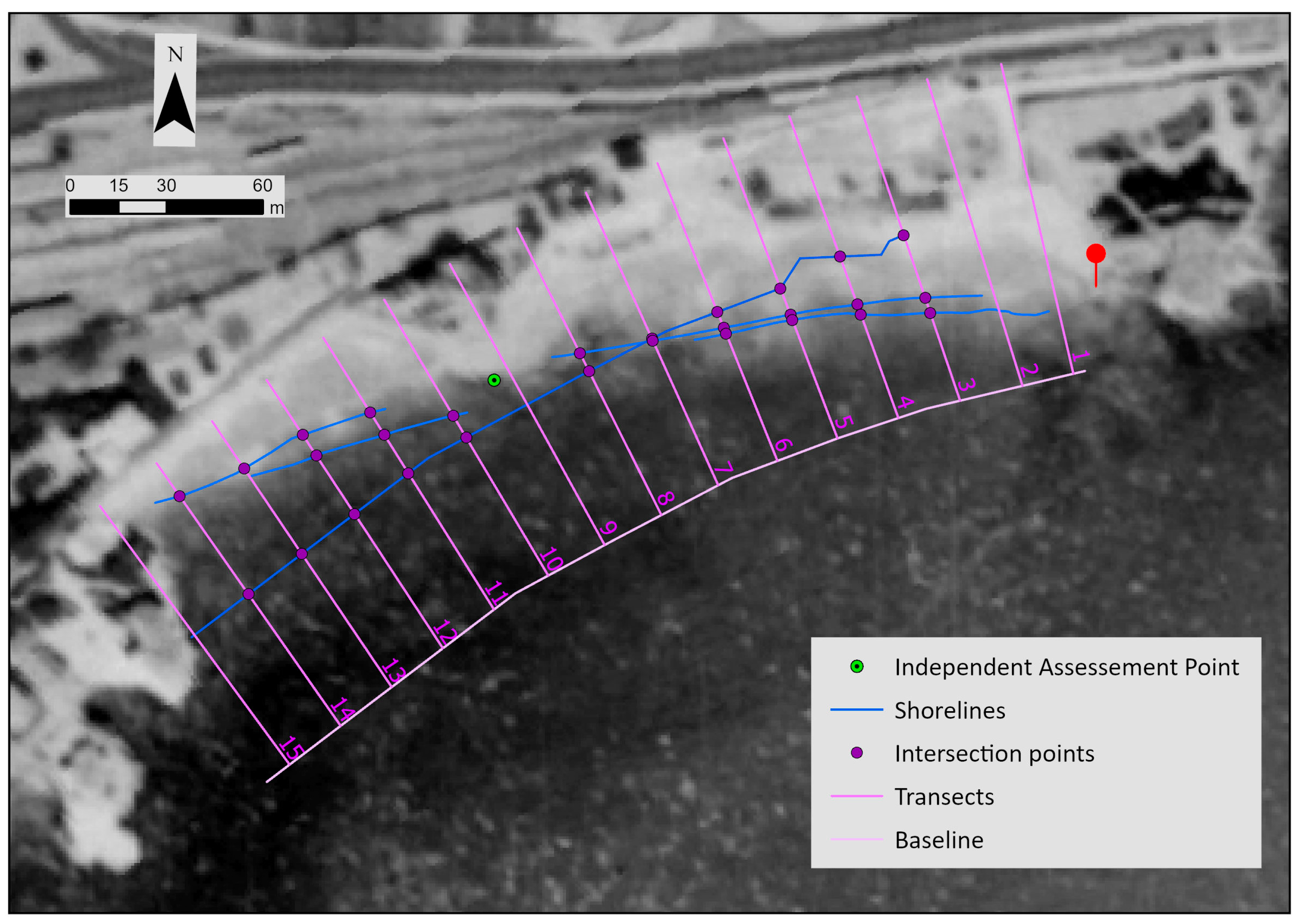
3.5. Shoreline Vectorization and Positional Change

After image rectification (Figure 10), each high-water line was manually vectorized (in ArcGIS Pro^®). The result were three line-vectors used for the shoreline change quantification process (Figure 12).

Differences in shoreline (SL) position were assessed using the Digital Shoreline Analysis System (DSAS)^® software v.6.0.168 [40], with an offshore baseline and 15 transects, spaced 20 m apart (Figure 12). This tool detects where each shoreline intersects a transect and then measures its distance to the baseline to calculate SL movement and evolution. The shorelines were grouped in pairs for estimating positional changes (movement) corresponding, in this case, to the three temporal windows: 30 years (from 1930 to 1960), 62 years (from 1960 to 2022), and 92 years (from 1930 to 2022). Due to the reduced number of shoreline positions, this study computed the net shoreline movement, i.e., the horizontal distance between two different lines/dates on each transect, signaling the relative position of the younger line in relation to the older one.

3.6. Uncertainty Estimation

In shoreline change analysis, several sources of error can affect the accuracy of shoreline positions and, depending on the objective/method, various sources can be identified and used in the quantification of total uncertainty [42]. In the present work, the positional uncertainty (U_year) associated with each shoreline extracted from each oblique image was estimated considering the contribution of errors related to the rectification process (E_r), the shoreline indicator (E_hwl), and the camera position (E_cam).

3.6.1. Error Associated with the Rectification Process (E_r)

The error associated with the rectification process (E_r) was estimated in two ways: using the survey data (ground control points (GCP)) and using an independent assessment.

Each GCP image position was independently rectified to its real-world coordinates, and the positional difference between rectification and field position was assessed, showing greater differences along the X direction (long-shore). As shoreline position analysis was performed in the cross-shore direction, the value used for the uncertainty was the mean of differences along this direction (Y direction). This analysis yielded a value of −0.24 m for the 2022 image. This value was also applied to the older dates.

To further strengthen the uncertainty analysis, an independent assessment was performed. A single common reference, recognizable in all images, was used because no other points were found suitable for this assessment. This point, located mid-distance along the beach and close to the shoreline (green dot in Figure 12), yielded Y-direction differences of 6.83 m, −4.08 m, and –1.34 m, respectively, for the 1930, 1960, and 2022 images.

The final E_r value was calculated as the sum of the absolute values of ground control points error and the reference point error, yielding the final values of 7.07 m, 4.32 m, and 1.58 m for 1930, 1960, and 2022, respectively (

Table 2. Quantified source of uncertainties (error type) for the analyzed dates (values in meters).

Error Type	1930	1960	2022
Rectification (Er) (m)	7.07	4.32	1.58
Indicator (EHWL) (m)	3.49	3.49	3.49
Camera position (Ecam) (m)	5.93	5.93	not applicable

).

3.6.2. High-Water Line Indicator Error (E_HWL)

The high-water line (HWL) indicator error is associated with assessing the Z_plane position in the rectification process by using the annual average of maximum high-tide elevation plus the contribution of sea level rise.

The E_HWL was assessed for the 2022 image as the mean horizontal positional difference between the HWL measured in the field and the HWL extracted from the rectification process using the 2022 master image, with a Z_plane value of 1.34 m (Table 1). This process yielded an average deviation of 3.24 m.

The 2022 high-water line measured in the field derives from a reconstruction of a three-dimensional model surveyed with an unmanned aerial vehicle (for X, Y position—orthomosaic, for Z position—digital elevation model (DEM)), the error associated with this procedure was also estimated and accounted for in estimating the final E_HWL value. The DEM error was estimated as the root mean square error of the differences between surveyed beach profiles and DEM values, yielding a 0.25 m positional error.

The final E_HWL is the sum of the error related to high-water line indicator and the DEM error (Table 2) with the final value of 3.49 m being applied to all the dates.

3.6.3. Camera Position Error (E_cam)

The camera position error is related to the differences in camera positions between the photographs of older times (different field views) and the master photograph. A test was made with two present-day photographs taken on each side (left and right) (~10 m) of CoastSnap Cascais station to mimic the slightly distinct perspective of the older photographs. The procedure co-registered the lateral photographs to the 2022 master, and the rectification process used a Z_plane elevation that corresponded to the mean height of the high-water line surveyed in the field. The average positional difference between the rectified shorelines and field shoreline yielded a value of 5.93 m (Table 2). We assumed this value to be the contribution of differences in camera positions in the overall estimation of the uncertainty for the historical photographs.

3.6.4. Estimation of Positional Uncertainty (U_year)

The positional uncertainty (U_year) was estimated with Equation (1), for the dates of 1930 and 1960 and with Equation (2) for the date of 2022 [41]. Results for the uncertainty of each shoreline are presented in

Table 3. Estimated uncertainties of shoreline position derived from ground photographs at Conceição-Duquesa beach, at each date (U_year).

	1930	1960	2022
Uncertainty (Uyear) (m)	±9.86	±8.13	±3.83

and represented as a gray buffer (see Figure in Section 4.1). The shoreline presenting the largest uncertainty is the 1930 with ± 9.86 m, followed by the 1960 with value ± 8.13 m, and the 2022 value ± 3.83 m.

$$U_{1930 1960} = \sqrt{E_r^2 + E_{HWL}^2 + E_{cam}^2}$$

(1)

$$U_{2022} = \sqrt{E_r^2 + E_{HWL}^2}$$

(2)

3.7. Validation

The validation procedure used 15 shoreline positions derived from other sources/dates. An analysis was performed using different NADIR images from the 20th and the 21st centuries:

(1)

a georeferenced 1948 photogrammetric 2D map (available in Oeiras City Council [43]);

(2)

georeferenced aerial imagery from 1958 and 1979 (provided by [41]);

(3)

orthoimages from 1995 and 2018 (publicly available at [29,44]) and 2000, 2002, 2005, 2007, 2008, 2009, 2010, 2013, 2015, and 2016 (kindly made available by Cascais City Council).

In each dataset, the wet–dry line was identified as a proxy of the high-water line and vectorized as line-vector. For each shoreline, the mean azimuth direction was assessed, allowing for the comparison of different shoreline positions and the identification of positional changes.

4. Results

4.1. Shoreline Position

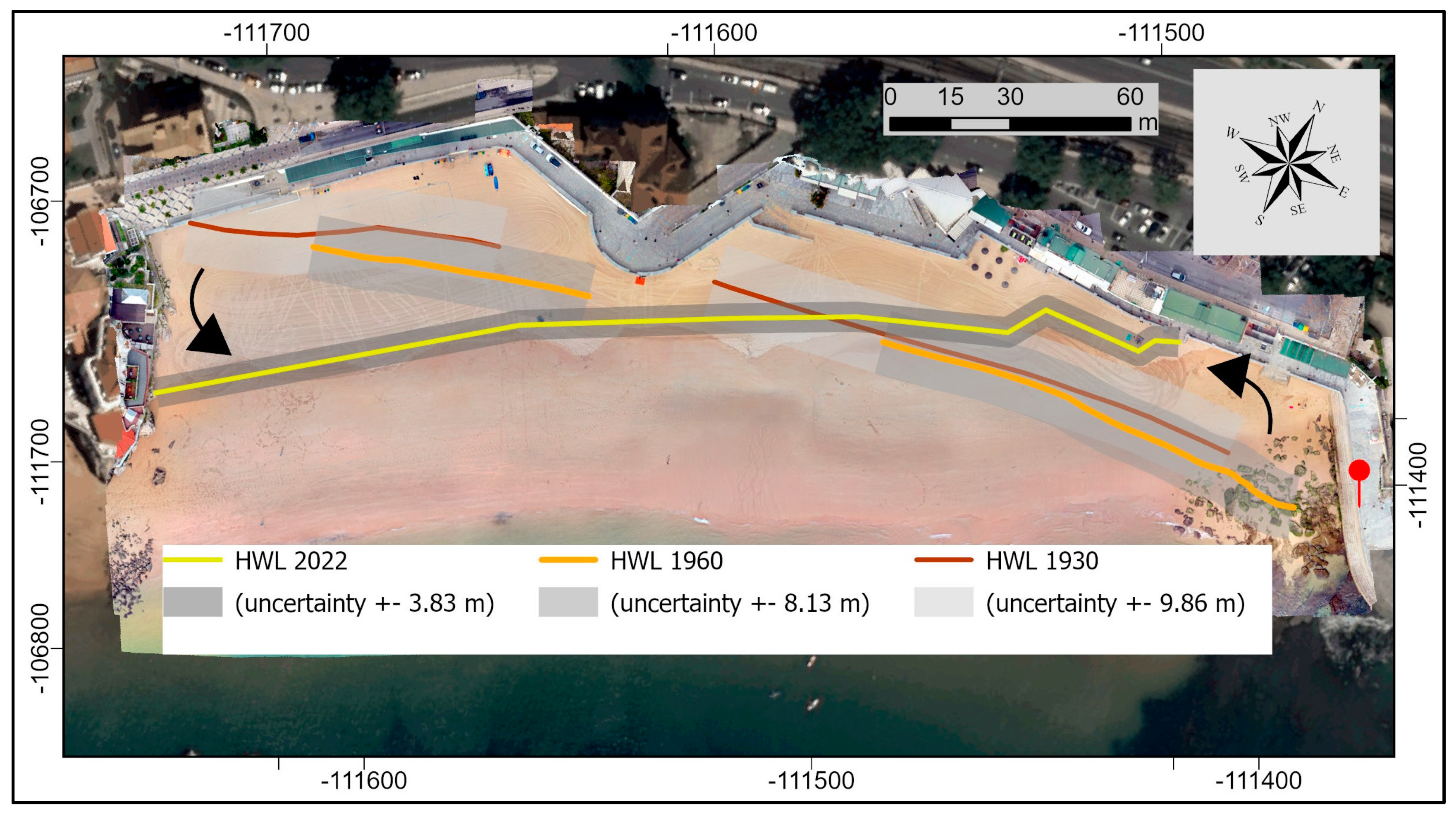
Figure 13 shows the rectified images for the 1930, 1960, and 2022 ground-oblique photographs, with the high-water line highlighted in red. The irregular appearance of the pixels is an artifact of the rectification process, during which the images are geometrically adjusted to align with a specified reference frame. This process can introduce visual distortions, particularly evident in the pixel structure. However, pre-highlighting the high-water line (HWL) position on the original images before undergoing image processing proves to be a significant advantage. By clearly delineating the HWL in advance, its position remains easily identifiable on the rectified images despite the introduced distortions.

It is important to note that the rectification process is influenced by relief displacement, meaning that only pixels at the selected elevation reference plane are accurately mapped. This limitation becomes apparent in the rectified images, as areas farther way from the shoreline—represented by the red high-water line—do not align perfectly with the base map data. These misalignments are a direct result of variations in elevation and perspective within the original oblique photographs, further emphasizing the importance of careful preprocessing and interpretation in rectification workflows.

Figure 14 illustrates the vectorized shorelines for the years 1930, 1960, and 2022, accompanied by the positional uncertainty for each dataset (U_year) represented by gray buffer zones (Table 3). The resulting shoreline positions reveal a notable consistency between the 1930 and 1960 datasets, both of which show similar spatial alignment. However, a marked contrast is observed when comparing these 20th-century shorelines to the 2022 dataset.

In the northeastern portion of Conceição-Duquesa (CD) beach, the shorelines from the older datasets (1930 and 1960) exhibit a more seaward position relative to the 2022 shoreline. Conversely, on the southwestern side of CD beach, this pattern is reversed, with the 2022 shoreline extending farther seaward than those from the earlier periods. This spatial shift creates a shoreline anticlockwise rotation. Notably, this apparent rotation appears to be cantered around the middle of the beach, in front of the prominent promenade round wall. The rotational shift shows comparable magnitudes for the northeastern and southwestern segments, albeit in opposite directions. The observed changes provide evidence of a significant shoreline adjustment (beach rotation) over the analyzed period and particularly between 1960 and 2022.

4.2. Quantitative Shoreline Change

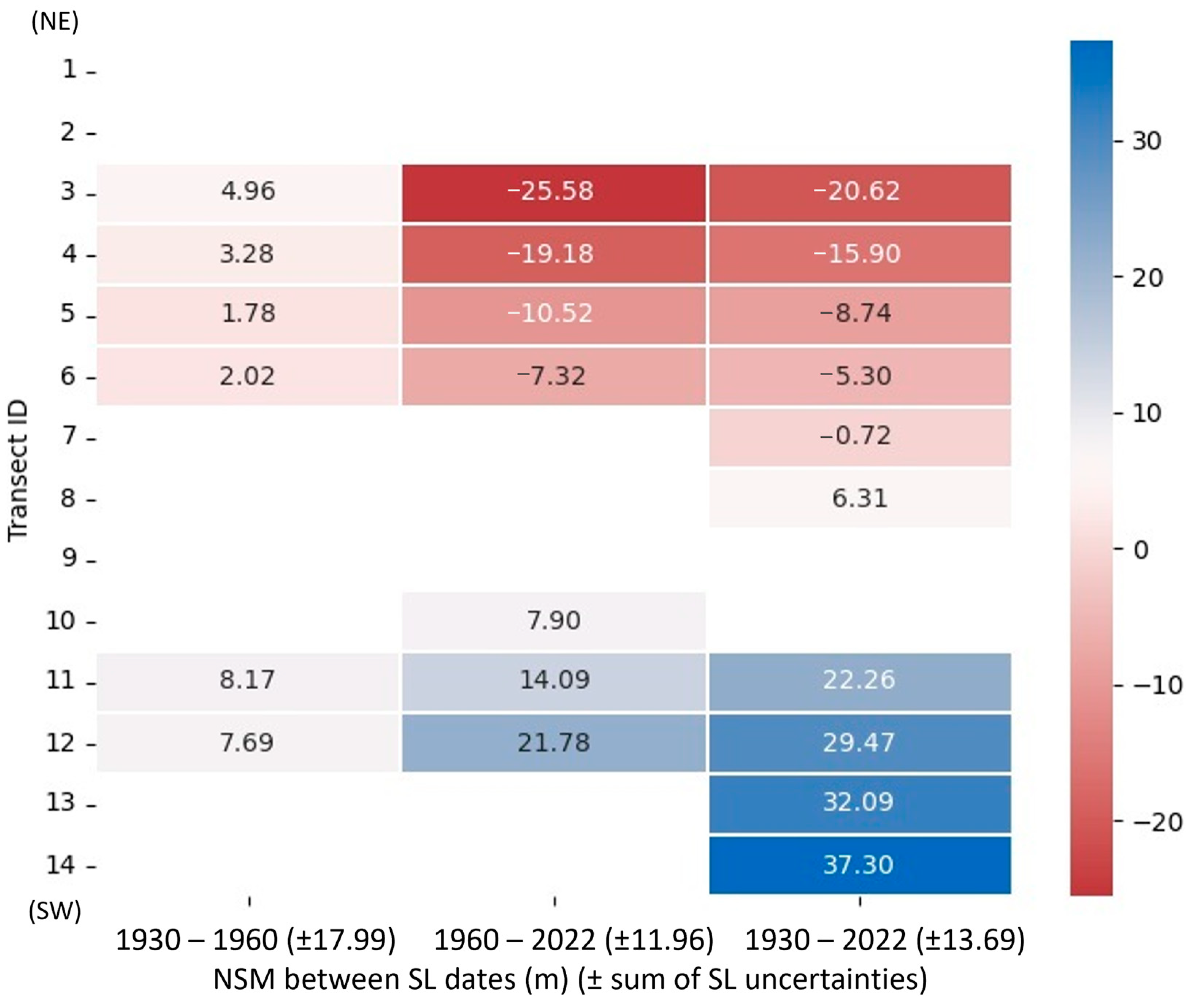
Figure 15 presents the Net Shoreline Movement (NSM) [40] values, measured in meters, across eight transects along Conceição-Duquesa beach for three distinct time intervals: 1930–1960, 1960–2022, and 1930–2022. The NSM values are visually represented using a color gradient, where red signifies shoreline retreat (negative values) and blue indicates shoreline advancement (positive values), providing a clear depiction of the direction and magnitude of shoreline change.

For the 1930–1960 interval, the results indicate a general pattern of shoreline retreat along the northeastern transects and shoreline advancement along the southwestern transects. However, the observed changes fall within the estimated uncertainty range for each shoreline position, suggesting that the beach can be considered stable during this period, with no significant net change in position.

The 1960–2022 interval displays a similar spatial pattern of retreat in the northeast and advancement in the southwest. However, during this later time limit, the magnitude of the changes is notably higher, with many of the observed shifts exceeding the uncertainty range. This provides robust evidence of a genuine shoreline rotation, specifically an anticlockwise rotation, with changes more clearly defined than in the earlier period.

When examining the longest interval, 1930–2022, the anticlockwise rotation of the shoreline becomes even more pronounced. The net shoreline movement for the southwestern transects shows significantly larger magnitudes compared to those in the northeastern sector. This highlights a marked and progressive shift in shoreline position over the last century, further emphasizing the rotational behavior of the beach system.

The analysis across these time intervals suggests that while short-term changes may occasionally fall within uncertainty margins, the long-term evolution of Conceição-Duquesa beach is characterized by a substantial and measurable shoreline adjustment.

4.3. Shoreline Position Validation

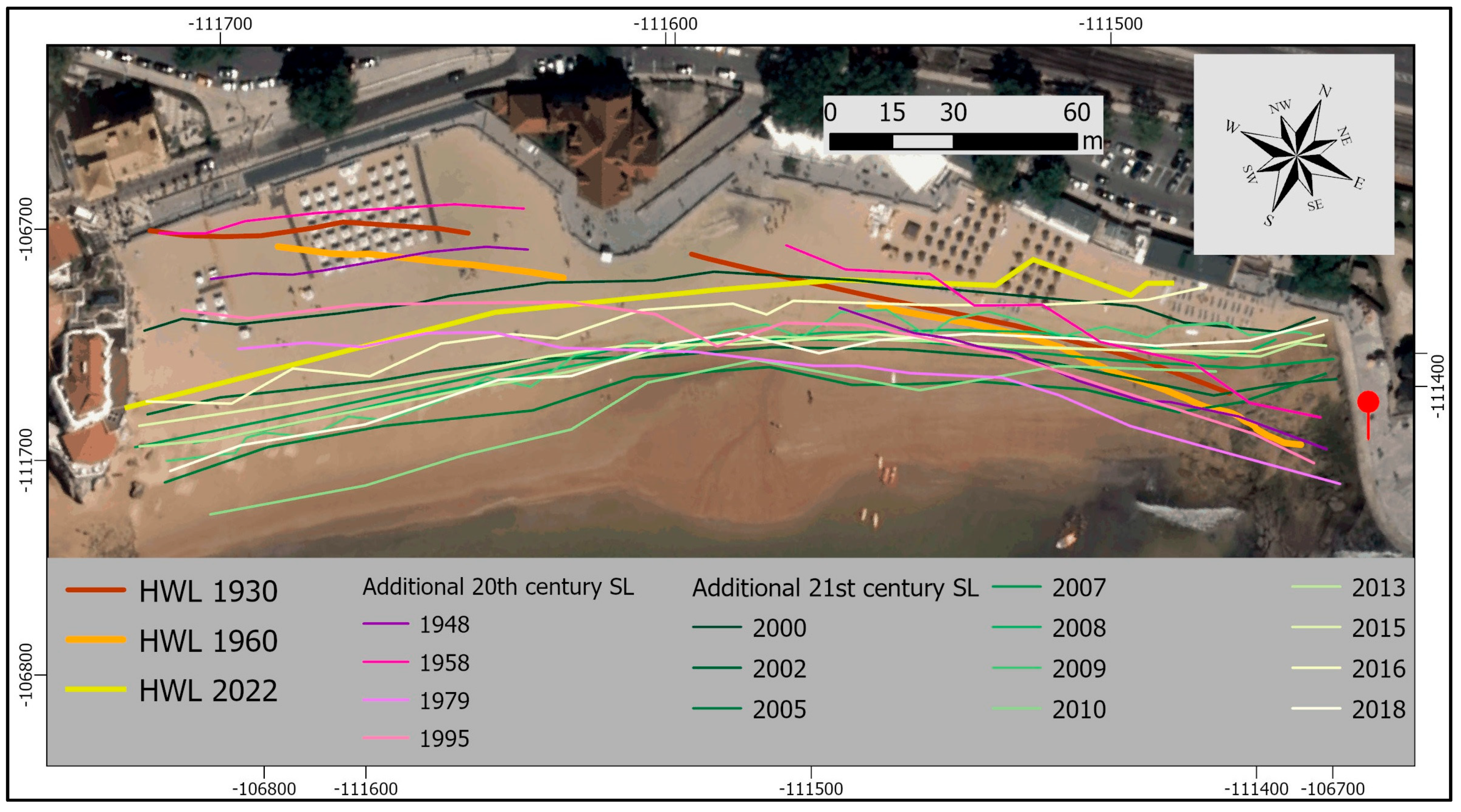
Figure 16 displays the high-water line (HWL) positions derived from additional sources (refer to Section 3.7. Validation): from the 20th-century (1948 (georeferenced photogrammetric 2D map), 1958 and 1979 (georeferenced aerial imagery), and 1995 (orthoimage)) and from the 21st-century (2000, 2002, 2005, 2007, 2008, 2009, 2010, 2013, 2015, 2016, and 2018) (orthoimages), alongside the datasets analyzed in detail in this study (1930, 1960, and 2022). A visual inspection of the data reinforces earlier findings: all 20th-century shorelines exhibit a spatial alignment similar to the older datasets analyzed in this study (1930 and 1960), confirming consistency in shoreline orientation throughout the 20th-century.

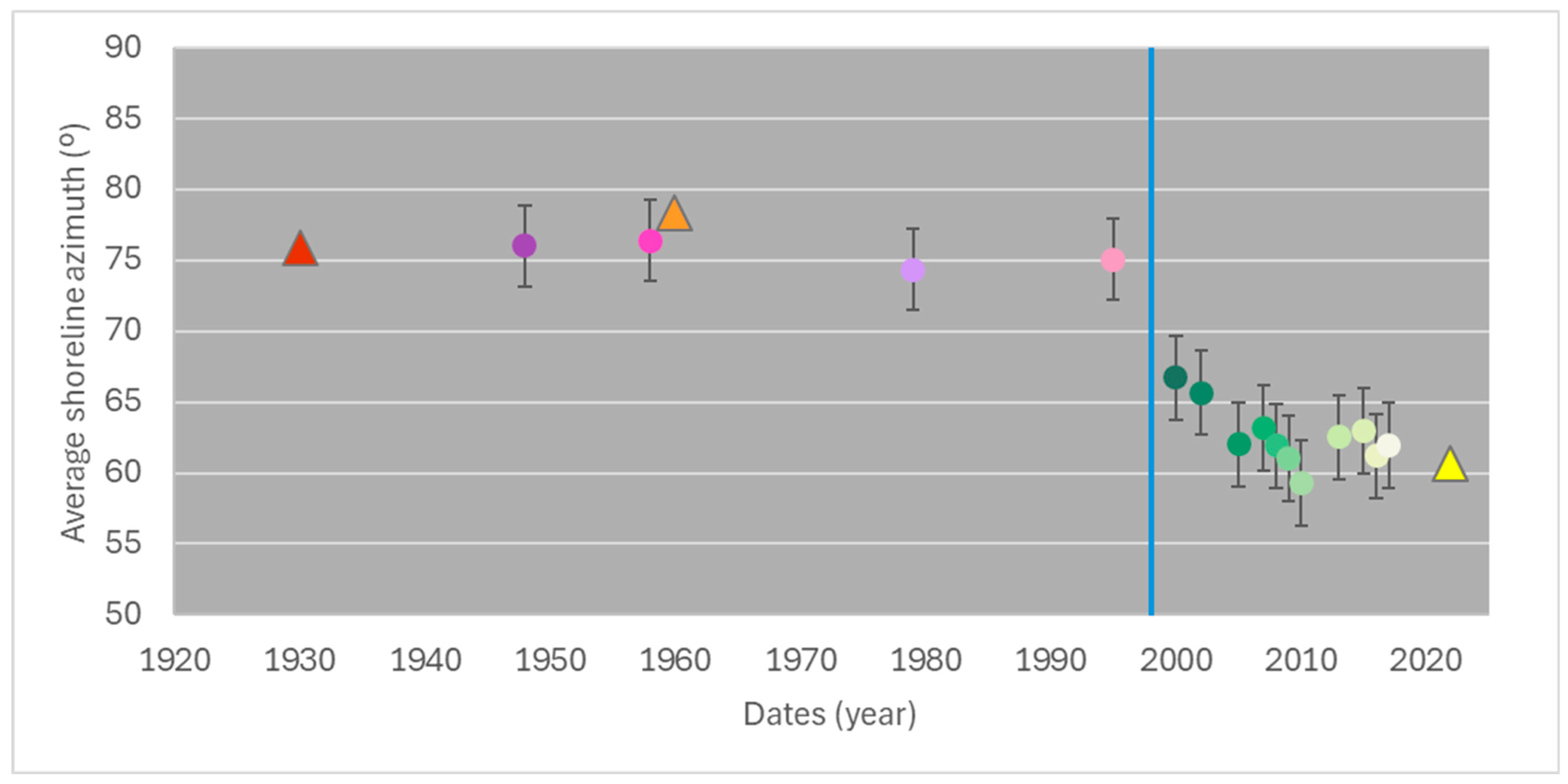
Figure 17 provides a quantitative summary of shoreline orientation by presenting the average azimuth direction for all high-water lines. The analysis identifies two distinct groups of shoreline directions: one corresponding to the 20th-century datasets with an average azimuth of 75°, and another corresponding to the 21st-century datasets with an average azimuth of 63°. These averages align with the detailed results from the primary datasets, where the 1930 and 1960 shorelines exhibit azimuth values of 76° and 78°, respectively, while the 2022 shoreline shows a substantially different azimuth of 61°.

The quantitative measurements of shoreline orientation corroborate the visual and qualitative observations. The shift in shoreline position over time clearly demonstrates a pattern of rotation, transitioning from the historical alignment observed in the 20th century to the distinctly altered orientation observed in the 21st century. This rotation is evident in the image datasets, which reveal a marked change in shoreline geometry from past to present. As such, beach rotation from historical data to recent data are not a seasonal signal or associated with singular events (storms), but a more prolonged and consistent long-term change signal.

The results provide compelling evidence of an anticlockwise rotation of Conceição-Duquesa beach’s shoreline, consistent across both qualitative and quantitative analyses. This rotation underscores a significant transformation in coastal dynamics over the past century.

5. Discussion

5.1. Shoreline Position Analysis and Implications for Coastal Dynamics

The shoreline positions derived from all ground-based datasets were successfully applied, demonstrating the efficacy of the proposed methodology. A comparison with traditional methods indicates that the new approach effectively replicates shoreline positions for older datasets. However, extracting shoreline positions from such datasets comes with certain limitations. The uncertainty assessment for these older ground-based photographs estimates an uncertainty of up to 10 m. Nevertheless, this level of uncertainty is comparable to that observed in traditional older datasets (e.g., [5,45,46,47]).

A relevant study by [48] investigated the impact of the Cascais marina construction, completed in 1998, on the adjacent coastline. The marina, located southwest of Conceição-Duquesa (CD) beach, was found to influence the nearshore wave regime and neighboring sandy beaches. Ref. [48] concluded that changes in wave energy flux induced by the marina resulted in a counterclockwise shoreline rotation at CD beach, with an estimated angular shift of 6°. The results presented in this study align with [48]’s findings, though the angular differences derived from shoreline positions based on aerial and ground-based images show values double those originally estimated using numerical modeling.

In 2005, Conceição-Duquesa beach underwent artificial nourishment [49]. This intervention significantly impacted the high-water line (HWL) position, corresponding to an increase in sand volume. As illustrated in Figure 17, there was a marked seaward shift in the shoreline from 2005 to 2022. Despite this trend, variations in shoreline position across different dates persist, likely due to the nature of the HWL used as a shoreline indicator. HWL is sensitive to short-term changes, and differences may also arise from the proxies used for HWL identification in the images and their correlation with specific elevations.

One consistent observation remains: the signal of beach rotation following the construction of the marina is evident and persistent over time. This long-term pattern underscores the significant impact of artificial coastal structures on shoreline dynamics, reinforcing the importance of integrating historical datasets and modern methodologies to assess and manage coastal changes effectively.

Long-term shoreline data based on often-overlooked historical source materials have added value in validating hindcast models, and the introduced methodology emerges as a powerful tool for local-scale shoreline studies. This methodology enables the validation of numerical models and supports the reinterpretation of past works, thereby bridging the gap between historical observations and modern coastal dynamics analyses.

5.2. Usage Notes

The proposed approach is straightforward and versatile, allowing the adaptation to other beach environments with minimal modifications. By meeting a few baseline requirements, the method can be applied to a wide range of beach systems, providing a valuable tool for historical shoreline analysis.

5.2.1. Minimum Requirements for Application

Beach System Characteristics

(1.1) The beach system should conform to an equilibrium beach profile, meaning that the cross-shore slope remains constant over time.

(1.2) No significant changes to the wave regime should have occurred during the analyzed period, as this ensures that shoreline positions derived from different datasets remain comparable.

(1.3) Changes in sea level, if applicable, must be accounted for to accurately align shoreline positions from different periods.

Historical Photographs or Images

(2.1) At least one historical photograph or image is required, where the snapshot viewpoint can be replicated in present time and ideally taken from a higher vantage point.

(2.2) The approximate location of the historical image’s viewpoint must be known. As a guide, images should be chosen to depict similar vanishing points (points to where parallel lines converge on the horizon in a perspective drawing or photograph). No formal analysis was performed to estimate a threshold value.

(2.3) For optimal results, historical images should depict cross-shore views of the beach and include identifiable landmarks visible in both the historical and present-day images.

5.2.2. Present-Day Datasets

A standard set of present-day data is necessary to enable the image rectification and shoreline extraction process:

(3.1) Present-Day Photographs: Contemporary photographs must be taken from the same viewpoint as the historical images. These photographs should be captured using a tripod or a fixed structure to ensure stability during image acquisition.

(3.2) Camera Parameters: Knowledge of the camera’s internal parameters is required to correct for distortions caused by camera optics. Various methodologies exist for estimating these parameters, as detailed in Section 3.4.3.

(3.3) Georeferencing Old (Historical) Images: Historical images must be georeferenced to the master image (present-day photograph) using standard GIS software or other software that allows effective co-registration. This step allows the integration of historical images into the workflow without requiring detailed knowledge of their original acquisition parameters.

(3.4) Ground Control Points: evenly spaced GCP comprising real-world coordinates and their corresponding positions in the image are essential for converting pixel coordinates into metric world coordinates. Further details on this process can be found in Section 3.4.3.

(3.5) Elevation of the Shoreline (Z-Plane): The elevation of the shoreline position must be specified for the rectification process, ensuring accurate transformation of historical image data.

5.2.3. Rectification and Workflow

The image rectification process can be executed using the COSMOS Python code, available at: https://github.com/RuiTaborda/COSMOS. This software enables the transformation of ground-based images into georeferenced, metrically accurate datasets for shoreline position analysis. However, other standard methods exist (e.g., [28,34,50]).

By satisfying these requirements, the proposed method offers a robust framework for extracting and analyzing shoreline positions from historical ground-based photographs. Its simplicity, adaptability, and reliance on widely available tools make it accessible to researchers and coastal managers. This method provides insights into long-term shoreline dynamics and extends the temporal range of analysis, offering a valuable perspective for understanding coastal evolution and informing sustainable management practices.

5.3. Future Work

Despite the success of the applied methodology, some space for improvement exists. Uncertainty estimation may include the error promoted by the larger pixel footprint as shoreline position is further away from the camera. This can be especially relevant for larger beaches (>500 m) and/or older image datasets with lower resolution. Also, because this study is estimating rotation changes, the uncertainty related with the azimuth difference in relation to the camera position could be assessed. Other tests that could improve the results would be to estimate the errors associated with the location of the common elements used to align the older with newer images could be estimated to assess the real impact of not having common points on the beach versus having more evenly spaced alignment points, different number of alignment points, among other possible sources of error.

6. Conclusions

The proposed method introduces a novel approach to leveraging historical ground-based photographs of beaches for shoreline position extraction, enabling quantitative analyses that extend further back in time compared to traditional datasets such as aerial photographs or satellite imagery (including modern analysis of satellite-derived shorelines). This methodology bridges the gap between historical and contemporary data by incorporating present-day information and technological capabilities to facilitate the use of older datasets in shoreline studies.

This study serves as a proof-of-concept approach, using a shore platform beach located in Cascais, central west coast of Portugal, and allowed to assess changes in shoreline position between 1930 and 2022. The high-water line position was successfully identified on each dataset, allowing identification of a beach rotation induced by anthropogenic actions. The morphodynamic changes inferred from analysis of historical, oblique images on postcards were successfully validated by comparison with other NADIR images from different dates. The methodology is easily replicated and applied to other beach systems, providing a valuable tool for historical shoreline analysis capable of complementing standard and more emergent datasets, including satellite imagery.