A Fast Satellite Selection Method Based on the Multi-Strategy Fusion Grey Wolf Optimization Algorithm for Low Earth Orbit Satellites

Abstract

Low Earth Orbit (LEO) satellites utilizing Doppler measurements can be an effective supplementary positioning solution when Global Navigation Satellite System (GNSS) signals are unavailable. LEO satellites pose challenges to the efficiency and stability of real-time satellite selection algorithms due to their high dynamic and large number. The traditional satellite selection algorithms have the problems of high computational complexity and significant hardware dependence. In contrast, the intelligent optimization algorithm significantly improves the accuracy and real-time performance of satellite selection through global search and efficient processing. According to the characteristics of LEO satellites, a Multi-Strategy Fusion Grey Wolf Optimization (MSFGWO) algorithm is proposed for satellite selection. The experimental results show that when six satellites are selected, the average Doppler Geometric Dilution of Precision (DGDOP) value of the MSFGWO algorithm is 222.08. Compared with the DGDOP ratio of the traversal method, it is 1.03. The three-dimensional positioning accuracy is 192.86 m, and the positioning error is improved by 54.43% compared with the positioning accuracy of the traditional GWO algorithm. The longest continuous observation was achieved for 45 s, during which no switching of six satellites occurred at adjacent moments. The calculation time of the algorithm was only 0.0174 s, and the efficiency was improved by 93.43%. The MSFGWO algorithm proposed in this paper not only improves the overall optimization ability of the Grey Wolf Optimizer (GWO) algorithm and effectively reduces the DGDOP value but also significantly reduces the satellite switching number and prolongates the continuous observation time, thus improving the stability and accuracy of the positioning solution.

1. Introduction

The Global Navigation Satellite System (GNSS) serves as the primary means for providing navigation and timing services on a global scale. However, given its inherent characteristics of signal openness and low receiving power, it remains susceptible to interference and deception in complex environments [1]. Consequently, there is a critical need for a backup navigation and positioning system with robust anti-interference capabilities. Low Earth Orbit (LEO) satellites, which possess the advantages of low transmission loss and latency due to their relatively low orbital altitude, have emerged as an effective supplementary positioning solution when GNSS are unavailable [2,3,4,5]. Currently, the global construction of LEO satellite constellations has entered a phase of rapid deployment. The Starlink constellation, developed by the US company SpaceX, has successfully achieved effective mitigation of self-interference among satellites through the implementation of advanced routing algorithms and optimized frequency allocation techniques [6,7]. The OneWeb constellation comprises a hybrid system of 720 satellites in orbit, designed to establish a low-latency and high-speed global communication network [8,9]. The Amazon Kuiper system is designed to deliver global network services utilizing a constellation of over 3000 satellites [10]. Projects such as China’s Apocalypse Constellation [11] and Qianfan Constellation [12] are currently being actively pursued and developed. These large-scale constellation deployments enable single-point observations to simultaneously capture dozens of satellites, thereby significantly enhancing the system’s service capabilities [13].

However, the dynamic characteristics of LEO satellites present significant challenges for the navigation and positioning system. The maximum duration of visibility for a single LEO satellite is limited to 10 to 15 min, and its rapid motion results in substantial Doppler frequency shifts. The low orbit reduces the duration of visibility over the ground, necessitating frequent switching between satellites or beams by ground user terminals. This not only compromises the continuity of communication but also has the potential to cause signal interruptions or degradation in quality. In addition, the limited availability of receiver channel resources, coupled with the necessity of frequent antenna adjustments for satellite tracking, further complicates the LEO satellite navigation and positioning system. Kassas et al. [14] and Khalife et al. [15,16] employed carrier phase tracking technology to precisely locate non-cooperative signals and successfully achieved meter-level positioning accuracy with Starlink constellation signals through utilizing the unmodulated carrier embedded in the signal header. However, the rapid motion of LEO satellites relative to ground receivers is susceptible to inducing Doppler frequency shifts, thereby complicating signal reception and processing. To address this challenge, carrier Doppler measurements are commonly employed for positioning purposes [17]. For the optimal selection of satellites in LEO satellite constellations, Moore et al. [18] formulated a minimization problem targeting Doppler Geometric Dilution of Precision (D-GDOP). Notably, DGDOP is influenced by the velocities and accelerations of the visible satellites.

When the number of phased array antennas is limited, it becomes essential to select satellite combinations that exhibit superior geometric configurations and extended visibility durations in real time. Optimizing the satellite selection algorithm can decrease the number of satellite switches, prolong continuous observability, and enhance the continuity and stability of satellite signal reception, as well as improve the precision of satellite navigation and positioning. The current research on satellite selection algorithms is primarily categorized into traditional geometric optimization algorithms and intelligent optimization-based satellite selection algorithms.

The traditional geometric optimization algorithm focuses on minimizing the Geometric Dilution of Precision (GDOP) as its primary objective and identifies the optimal satellite combination by evaluating geometric configurations [19]. Traditional methods include the maximum tetrahedral volume approach, the elevation angle threshold approach, and so on. Zhang et al. [20] utilized the principle of maximizing elevation angle and ensuring uniform azimuth angle distribution, thereby effectively reducing traversal time. Peng et al. [21] achieved a uniform distribution of satellites by employing a method that involved grouping based on elevation angles and uniformly selecting azimuth angles. Shi et al. [22] integrated the Sherman–Morrison formula with the maximum-volume tetrahedron method, thereby achieving an efficiency enhancement under the 11-satellite threshold. However, conventional satellite selection algorithms solely focus on geometric distribution while neglecting critical influencing factors such as signal strength, multipath error, and visible satellite duration. Additionally, the computational complexity grows exponentially with an increasing number of satellites, thereby imposing higher demands on the receiver’s hardware capabilities and failing to satisfy real-time processing requirements.

The intelligent optimization algorithm employs a heuristic global search strategy. By leveraging the population evolution mechanism, it successfully reduces algorithmic complexity, thereby significantly enhancing computational efficiency and diminishing the hardware requirements for the receiver. This algorithm is particularly well-suited for real-time positioning tasks that have low accuracy demands and utilize cost-effective receiver equipment. Song et al. [23] proposed a multi-constellation genetic algorithm (GA)-based satellite selection method, which avoids falling into local optima by preferentially selecting chromosomes during the crossover process. Wang et al. [24,25] successively introduced the Chaos Particle Swarm Optimization (CPSO) algorithm and the Artificial Fish Swarm Algorithm–Particle Swarm Optimization (AFSA-PSO) algorithm. The performance of these algorithms was improved by leveraging chaos mapping for initialization and utilizing the global search capabilities of the Artificial Fish Swarm Algorithm. Yang et al. [26] employed the Harris Hawks Optimization (HHO) algorithm, leveraging its dynamic exploration and exploitation mechanism with adaptive switching to facilitate rapid satellite selection in multi-GNSS systems. Qiu et al. [27] developed a dual-objective model combining Geometric Dilution of Precision (GDOP) and satellite selection number using the Imperialist Competitive Algorithm (ICA), enhancing decision-making flexibility by incorporating prior constraints on elevation and azimuth angles. Although these algorithms improve computational efficiency and reduce complexity, intelligent optimization-based satellite selection algorithms typically encounter issues such as extensive initial parameter configurations, susceptibility to local optima, and reliance on a singular satellite selection criterion. Yu et al. [28] reduced the computational complexity and enhanced the efficiency of satellite selection by incorporating an adaptive convergence factor into the Grey Wolf Optimizer (GWO) algorithm. The GWO algorithm is particularly well-suited for the application of satellite selection algorithms in complex environments, such as LEO satellite constellations, owing to its advantages of low computational complexity, ease of implementation, and minimal parameter adjustments.

For the above issues, this paper proposes a Multi-Strategy Fusion Grey Wolf Optimization (MSFGWO) algorithm, which is designed to enhance dynamic adaptability and computational efficiency in the process of selecting LEO satellites. By incorporating geometric configuration optimization, computational efficiency enhancement, and visible satellite time maximization, the limitations of traditional single-index optimization are effectively overcome. This approach not only reduces the hardware requirements for receivers but also improves the real-time performance, stability, and accuracy of navigation and positioning in complex environments.

2. MSFGWO Algorithm Model

The MSFGWO method integrates the GWO algorithm with a hybrid approach that incorporates the perturbation mechanism of the Variable Neighborhood Search (VNS) algorithm, the GA mutation strategy, and the Entropy Weight Method (EWM). This integration addresses the issues of low population diversity and susceptibility to local optima in the GWO algorithm, as well as mitigating the frequent satellite switching problem commonly encountered with LEO satellites. The MSFGWO method employs the Doppler Geometric Dilution of Precision (DGDOP) value as the fitness function for optimization.

2.1. GWO Algorithm

The GWO algorithm attains its optimization objectives through emulating the predatory behavior of grey wolf populations and leveraging the cooperative mechanisms within the group [29]. Based on the hierarchical structure of the wolf pack, the $\alpha$ wolf—as the leader—assumes a pivotal role in directing the hunting process. The $\beta$ and $\delta$ wolves relay the $\alpha$’s directives and assist in the search for prey, while the $\omega$ wolf, positioned at the lowest rank, participates in the hunt by adhering to instructions. In the context of optimal solution identification, the $\alpha$ wolf signifies the optimal solution, the $\beta$ wolf represents the second-best solution, and the $\delta$ wolf denotes the third-best solution. Meanwhile, the $\omega$ wolf contributes to the exploration of all potential solutions.

During the process of hunting prey, the distance between an individual grey wolf and their prey is calculated according to Equation (1), while their positions are updated as shown in Equation (2) [29]:

$$\overrightarrow{D}=\left|\overrightarrow{C}·{\overrightarrow{X}}_P(\mathrm{t})-\overrightarrow{X}(t)\right|,$$

(1)

$$\overrightarrow{X}(t+1)={\overrightarrow{X}}_P(t)-\overrightarrow{A}·\overrightarrow{D},$$

(2)

$$\overrightarrow{A}=2\overrightarrow{a}·{\overrightarrow{r}}_1-\overrightarrow{a},$$

(3)

$$\overrightarrow{C}=2·{\overrightarrow{r}}_2,$$

(4)

where t is the current iteration; ${\overrightarrow{X}}_P(t)$ and $\overrightarrow{X}(t)$ represent the positions of the prey and wolf in the t-th iteration, respectively; $\overrightarrow{A}$ and $\overrightarrow{C}$ are parameters; $\overrightarrow{a}$ represents a convergence factor; and ${\overrightarrow{r}}_1$ and ${\overrightarrow{r}}_2$ are random vectors.

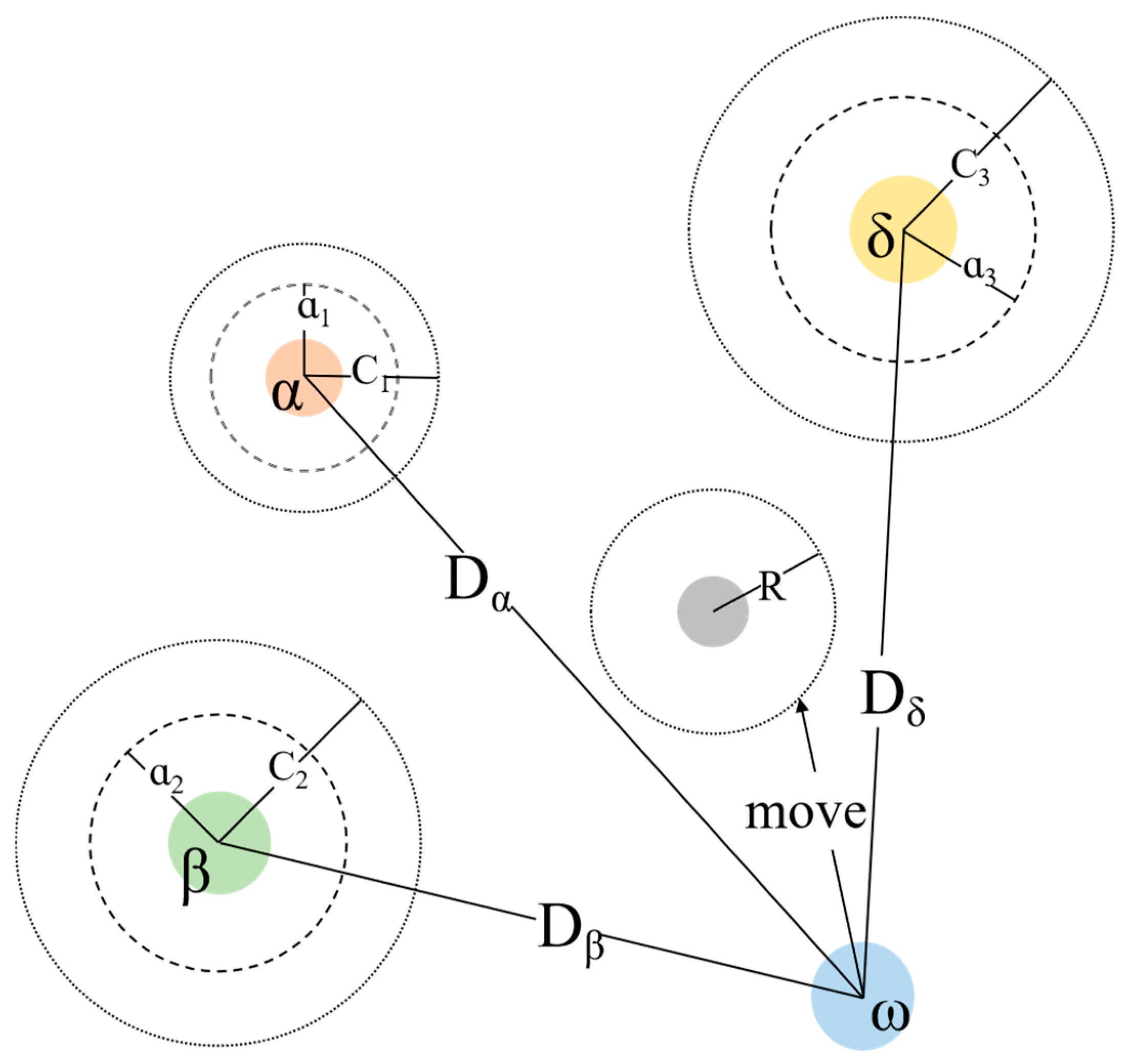
During the hunting process, the $\omega$ wolf executes its hunting activities in coordination with $\alpha$, $\beta$, and $\delta$ wolves, following their leadership. The $\omega$ wolf dynamically adjusts its position based on the actions of the $\alpha$, $\beta$, and $\delta$ wolves as detailed in Equations (5)–(7) [29]:

$$\left\{\begin{array}{c}{\overrightarrow{D}}_a=\left|{\overrightarrow{C}}_1·{\overrightarrow{X}}_a-\overrightarrow{X}\right|\\ {\overrightarrow{D}}_{\beta }=\left|{\overrightarrow{C}}_2·{\overrightarrow{X}}_{\beta }-\overrightarrow{X}\right|\\ {\overrightarrow{D}}_{\delta }=\left|{\overrightarrow{C}}_3·{\overrightarrow{X}}_{\delta }-\overrightarrow{X}\right|\end{array}\right.,$$

(5)

$$\left\{\begin{array}{c}{\overrightarrow{X}}_1={\overrightarrow{X}}_a(t)-{\overrightarrow{A}}_1·{\overrightarrow{D}}_a\\ {\overrightarrow{X}}_2={\overrightarrow{X}}_{\beta }(t)-{\overrightarrow{A}}_2·{\overrightarrow{D}}_{\beta }\\ {\overrightarrow{X}}_3={\overrightarrow{X}}_{\delta }(t)-{\overrightarrow{A}}_3·{\overrightarrow{D}}_{\delta }\end{array}\right.,$$

(6)

$$\overrightarrow{X}(t+1)={\displaystyle \frac{{\overrightarrow{X}}_1+{\overrightarrow{X}}_2+{\overrightarrow{X}}_3}{3}}.$$

(7)

In Equation (5), ${\overrightarrow{D}}_a$, ${\overrightarrow{D}}_{\beta }$, and ${\overrightarrow{D}}_{\delta }$ represent the distances between the $\omega$ wolf and the $\alpha$, $\beta$, and $\delta$ wolves, respectively; ${\overrightarrow{C}}_1$, ${\overrightarrow{C}}_2$, and ${\overrightarrow{C}}_3$ are random numbers within the range of [0, 1]; and ${\overrightarrow{X}}_a$, ${\overrightarrow{X}}_{\beta }$, ${\overrightarrow{X}}_{\delta }$, and $\overrightarrow{X}$ represent the current positions of the $\alpha$, $\beta$, $\delta$, and $\omega$ wolves, respectively. Equation (6) represents the direction and stride of the movement of the $\alpha$, $\beta$, and $\delta$ wolves. Equation (7) represents the final position update for the $\omega$ wolf, based on the movements of the $\alpha$, $\beta$, and $\delta$ wolves. The process of updating the position of the $\omega$ wolf in relation to the $\alpha$, $\beta$, and $\delta$ wolves within the wolf pack is illustrated in Figure 1.

2.2. Fitness Function DGDOP

Due to the adoption of the Doppler positioning method in LEO positioning, the basic observation equation for Doppler positioning is given by Equation (8) [30]:

$$\dot{\rho }=(v_r-v^s){\displaystyle \frac{x^s-x_r}{\parallel x^s-x_r\parallel }}+c(\dot{\delta }{t}_r-\dot{\delta }{t}^s)+{\epsilon }_{\dot{\rho }},$$

(8)

where $\dot{\rho }$ represents the pseudo-range rate, which is the Doppler observation in units of m/s; $\dot{\delta }{t}^s$ and $\dot{\delta }{t}_r$ represent the temporal derivatives of the satellite clock bias and receiver clock bias, respectively; ${\epsilon }_{\dot{\rho }}$ represents random noise in the Doppler observations; $x_r={[\begin{array}{ccc}{x}_r& y_r& z_r\end{array}]}^{\mathrm{T}}$ and represents the position and velocity of the receivers, respectively; $x^{\mathrm{s}}={[\begin{array}{ccc}{x}^{\mathrm{s}}& y^{\mathrm{s}}& z^{\mathrm{s}}\end{array}]}^{\mathrm{T}}$ and ${\nu }^s=[\begin{array}{ccc}{\nu }_x^s& {\nu }_y^s& {\nu }_z^s]\end{array}$ represent the position and velocity of the satellite, respectively.

For n satellites, this can be written in matrix form, as follows:

$$G·\Delta u=b,$$

(9)

$${\left[\begin{array}{cccc}{\displaystyle \frac{\partial {\dot{\rho }}^{s_1}}{\partial x}}& {\displaystyle \frac{\partial {\dot{\rho }}^{s_1}}{\partial y}}& {\displaystyle \frac{\partial {\dot{\rho }}^{s_1}}{\partial z}}& 1\\ {\displaystyle \frac{\partial {\dot{\rho }}^{s_2}}{\partial x}}& {\displaystyle \frac{\partial {\dot{\rho }}^{s_2}}{\partial y}}& {\displaystyle \frac{\partial {\dot{\rho }}^{s_2}}{\partial z}}& 1\\ ⋮& ⋮& ⋮& ⋮\\ {\displaystyle \frac{\partial {\dot{\rho }}^{s_n}}{\partial x}}& {\displaystyle \frac{\partial {\dot{\rho }}^{s_n}}{\partial y}}& {\displaystyle \frac{\partial {\dot{\rho }}^{s_n}}{\partial z}}& 1\end{array}\right]}_{x=x_k}\left[\begin{array}{c}{x}_{k+1}-x_k\\ y_{k+1}-y_k\\ z_{k+1}-z_k\\ \delta t_{rk+1}-\delta t_{rk}\end{array}\right]=\left[\begin{array}{c}{\dot{\rho }}^{s_1}(\mathit{u})-{\widehat{\dot{\rho }}}^{s_1}({\mathit{u}}_k)\\ {\dot{\rho }}^{s_2}(\mathit{u})-{\widehat{\dot{\rho }}}^{s_2}({\mathit{u}}_k)\\ ⋮\\ {\dot{\rho }}^{s_n}(\mathit{u})-{\widehat{\dot{\rho }}}^{s_n}({\mathit{u}}_k)\end{array}\right],$$

(10)

In Equations (9) and (10), $G$ represents the coefficient matrix of the positioning system; ${\displaystyle \frac{\partial {\dot{\rho }}^{s_n}}{\partial x}}$, ${\displaystyle \frac{\partial {\dot{\rho }}^{s_n}}{\partial y}}$, and ${\displaystyle \frac{\partial {\dot{\rho }}^{s_n}}{\partial z}}$ represent the Doppler observations ${\dot{\rho }}^{s_n}$ of the receiver with respect to satellite n in terms of partial derivatives with respect to x, y, and z, respectively, at an initial estimate point ${\mathit{u}}_k$; $b$ is the Doppler shift change amount; ${\dot{\rho }}^{s_n}(\mathit{u})$ and ${\widehat{\dot{\rho }}}^{s_n}({\mathit{u}}_k)$ represent the actual measured Doppler value and predicted value for satellite n by the receiver, respectively.

The matrix $Q$ is defined as an amplification factor for Doppler measurement errors.

$$Q={(G^{\mathrm{T}}G)}^{-1}=\left[\begin{array}{cccc}{q}_{11}& q_{12}& q_{13}& q_{14}\\ q_{21}& q_{22}& q_{23}& q_{24}\\ q_{31}& q_{32}& q_{33}& q_{34}\\ q_{41}& q_{42}& q_{43}& q_{44}\end{array}\right].$$

(11)

Therefore, the DGDOP of Doppler positioning can be determined accordingly:

$$\mathrm{DGDOP}=\sqrt{q_{11}+q_{22}+q_{33}+q_{44}}.$$

(12)

2.3. Hybrid Algorithm

2.3.1. Improvement of the Search Mechanism

In the position update process of the GWO algorithm, the majority of grey wolf individuals within the population converge towards the optimal, sub-optimal, and third-best solutions. This convergent behavior results in the individual grey wolves within the population gradually becoming homogeneous, thereby diminishing the population diversity and narrowing the scope of exploration. Consequently, this hinders the discovery of new, potentially superior solution spaces, ultimately limiting the algorithm’s performance when considering complex optimization problems. Furthermore, while the GWO algorithm establishes an effective mechanism for balancing exploration and exploitation through the parameters $\overrightarrow{a}$ and $\overrightarrow{A}$, its exploration capability remains heavily reliant on the parameter C. This singular dependence on $\overrightarrow{C}$ for exploration increases the likelihood of the algorithm converging to local optima, thereby hindering its ability to effectively search for the global optimum. To address the aforementioned challenges, the proposed algorithm incorporates the perturbation mechanism of the VNS algorithm and the mutation strategy of the GA.

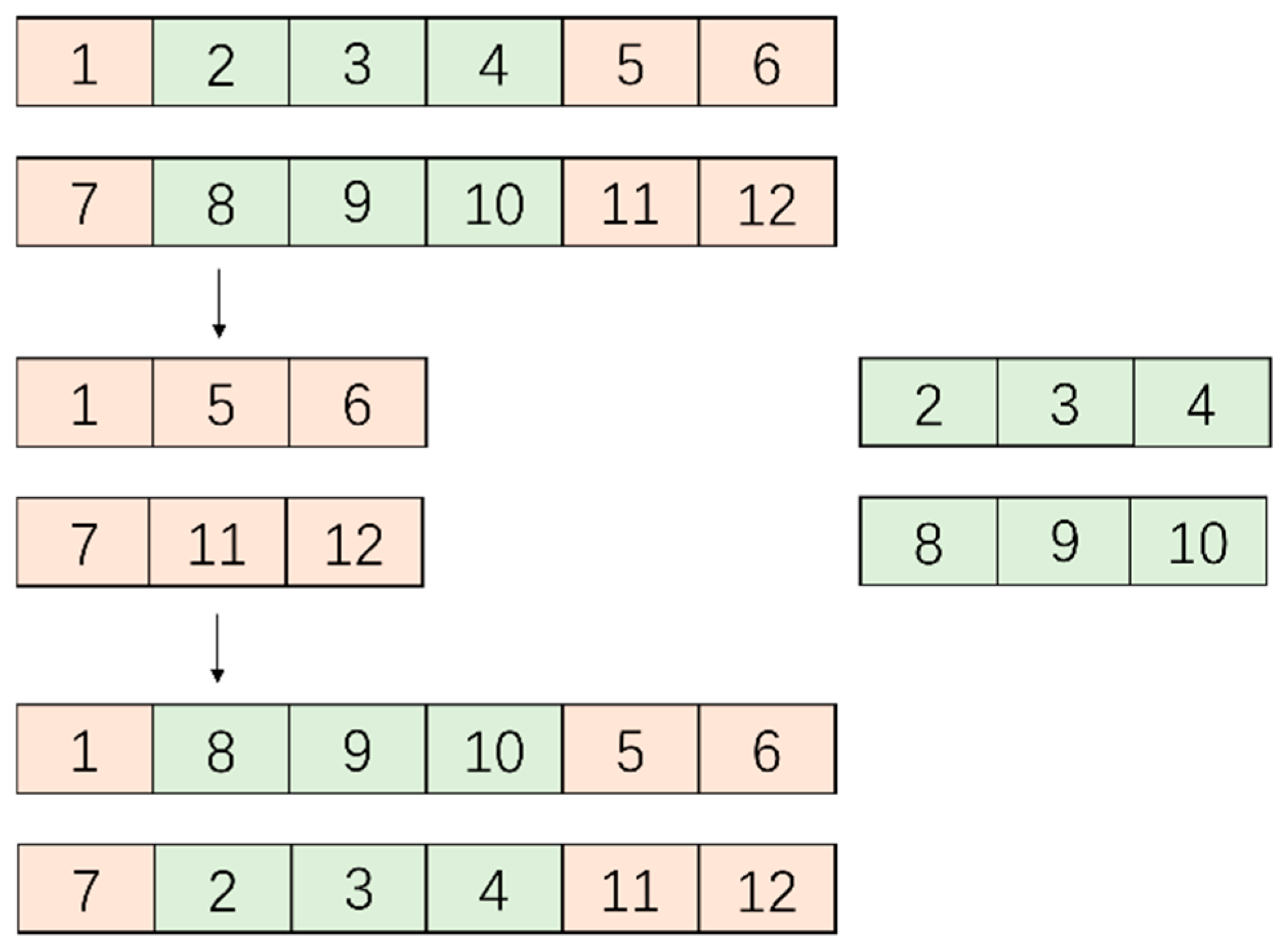
1.

Shaking Procedure in VNS Algorithm

The shaking procedure within the VNS algorithm serves to modify the spatial configuration among the grey wolf individuals. This study employs the satellite exchange method to generate new grey wolf individuals, effectively mitigating the tendency of grey wolf individuals in the GWO algorithm to gradually converge. This enhancement improves the algorithm’s capability to explore a broader solution space. This operation not only enhances the GWO algorithm’s ability to avoid local optima but also substantially increases the population diversity. The shaking procedure in the VNS algorithm is depicted in Figure 2.

2.

Mutation Strategy in GA

The mutation strategy in the GA is implemented by randomly altering elements within the individual grey wolf representations. In this study, the satellite combinations associated with each grey wolf are stochastically reconfigured to generate novel grey wolf entities. This process not only effectively enhances the population diversity but also substantially improves the algorithm’s capability to explore a broader solution space. Consequently, this assists the GWO algorithm in avoiding entrapment in local optima. The mutation strategy in the GA is shown in Figure 3.

2.3.2. Entropy Weight Method

The EWM is a widely recognized approach for determining objective weights. It calculates the entropy values of indicators based on the impacts of numerical changes in each indicator on the overall system, thereby assigning appropriate weights to each indicator. In this study, we utilize the EWM method, considering two critical indicators: the DGDOP values of grey wolf individuals at adjacent moments and the observable time of each satellite they represent. This approach allows for optimization of the final satellite selection results. The application of the EWM method not only effectively reduces the frequency of satellite switching between adjacent moments, thereby mitigating issues such as signal interruption and data instability caused by frequent switching, but also extends the continuous observation time of the same group of satellites. This provides more stable and continuous data support for positioning solution calculations, significantly enhancing both the stability and accuracy of these calculations.

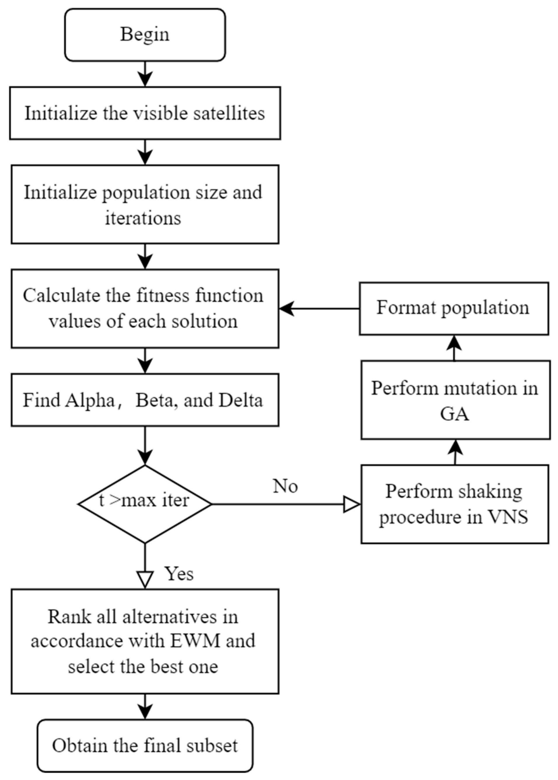
2.4. Steps of MSFGWO Algorithm

The proposed MSFGWO algorithm incorporates the perturbation mechanism of the VNS algorithm and the mutation strategy of the GA to enhance the overall optimization capability of the GWO algorithm. Additionally, the EWM method is employed to minimize the satellite handover frequency between consecutive time intervals, thereby extending the continuous observation duration. This results in improved stability and accuracy of the obtained positioning solutions.

Step 1: Filter all available satellites with elevation angles greater than 10° and assign them numbers. Set the number of selected satellites to n, based on the receiver’s channel count.

Step 2: Set the initial population size and iteration times for the MSFGWO algorithm.

Step 3: Calculate the DGDOP values of various satellite combinations in the initial population, and select the initial $\alpha$, $\beta$, and $\delta$ wolves based on their fitness values.

Step 4: Apply the shaking procedure from the VNS method to each satellite combination in the initialized population.

Step 5: Perform the GA mutation strategy on each combination of satellites obtained in Step 3.

Step 6: Use the results obtained through these operations as new populations and calculate DGDOP values for each satellite selection scheme while updating the wolves in the population.

Step 7: Determine whether the maximum number of iterations has been reached or not; if not, repeat Steps 3–5; if yes, proceed to Step 7.

Step 8: Evaluate and select the final selection scheme based on the EWM, combining previous and current selection results, DGDOP values, and the visibility time of selected satellites.

Accordingly, the flowchart of the MSFGWO algorithm is shown in Figure 4.

3. Parameter Selection for the MSFGWO Algorithm

A simulation experiment was conducted using the Starlink constellation. The data from the Starlink constellation on 19 July 2024 were used, with the ground point set at Zhengzhou (N34.76°, E113.65°) and an observation elevation angle of 10°. A total of 6623 Starlink satellites were simulated, with satellite data updated every second and a duration of one hour for observation (equivalent to 3600 s). On average, there were 13.68 satellites visible per second in the simulation experiment, with a maximum visibility of up to 20 satellites and a minimum visibility of 7 satellites.

3.1. Population Size and Iterations

The performance of the GWO algorithm is closely related to the population size and the number of iterations. The population size affects the calculation accuracy, while the number of iterations affects the calculation efficiency. Over the hour-long experiment, an average of 13.68 satellites could be observed per second. Therefore, for the parameter experiments, data from the 138th second were used, taking 14 visible satellites as a basis for setting parameters in this magnitude range. In the traversal method, it was set to take four satellites and calculate DGDOP values $C_{14}^4=1001$ times. The optimal DGDOP value obtained was 312.8203, with a time consumption of 0.0408 s.

3.1.1. Effects of Population Size

The experiment was conducted with 20 iterations, with the population size ranging from 1 to 10 with a step of 1. Four satellites were selected, and the Monte Carlo experiment was repeated 50 times to obtain the average value. The impact of population size on the algorithm’s performance was analyzed, as detailed in Figure 5 and Figure 6.

Combining Figure 5 and Figure 6, as the population size increases, the average DGDOP value gradually approaches the optimal selection result of the exhaustive method. The average DGDOP value decreased from 444.3042 to 384.1425, with an average error reduction from 42.03% to 22.80%, while the time consumption increased from 0.0251 s to 0.0777 s. From Figure 5 and Figure 6, it is evident that when the population size was set to five, both the average DGDOP and DGDOP average error significantly decreased while time consumption showed linear growth. Therefore, selecting a population size of five will result in less time consumption and a closer approximation of DGDOP values when compared to those obtained using the exhaustive method.

3.1.2. Effects of Number of Iterations

Next, the population size was set to five, with the number of iterations ranging from 1 to 20 in increments of one. Four satellites were selected, and the Monte Carlo experiment was repeated 50 times to obtain the average value. The influence of the number of iterations on the algorithm’s performance was analyzed, as shown in Figure 7 and Figure 8.

Combining Figure 7 and Figure 8, when the initial population size is fixed, with an increase in the number of iterations, the average DGDOP value gradually approaches the optimal satellite selection result obtained using the exhaustive search method. The average DGDOP value decreased from 437.9925 to 399.9498, and the average DGDOP error decreased from 40.01% to 27.85%. Meanwhile, the time computation increased from 0.0042 to 0.0422 s. From Figure 7 and Figure 8, it can be clearly seen that although there was a significant decrease in average DGDOP at iteration number 11, the error rate only decreased from 40.01% to 30.96%, while the computation time increased by a factor of approximately 4.57 times; when the number of iterations was set to seven, the error rate decreased from 40.01% to 35.17%, while the computation time increased by a factor of approximately 2.57 times. Therefore, considering the balance between DGDOP values and computational time, the number of iterations should be set as seven, which results in lower computational time while maintaining the DGDOP value close to the optimal satellite selection result.

In summary, using the MSFGWO algorithm with a population size of five and an iteration number of seven can ensure accurate satellite selection while achieving fast and efficient selection of optimal visible satellite configurations.

4. Simulation and Analysis

The simulation experiment utilized the Starlink constellation; specifically, the data from the Starlink constellation on 19 July 2024 were employed. The ground station was located in Zhengzhou (34.76°N, 113.65°E), with an observation elevation angle of 10 degrees. A total of 6623 Starlink satellites were included in the simulation. Satellite data were generated at one-second intervals, and the observation period spanned one hour (for a total of 3600 s).

To evaluate the satellite selection performance of the proposed MSFGWO algorithm, a comparative analysis was conducted using the traversal method, GWO algorithm, Strategy Fused Grey Wolf Optimization Algorithm A (SFGWO-A), Strategy Fused Grey Wolf Optimization Algorithm B (SFGWO-B), and the MSFGWO algorithm. Specifically, SFGWO-A enhances the global search capability through integrating the perturbation operation from the VNS algorithm and the mutation strategy from the GA into the traditional GWO framework, while SFGWO-B incorporates the EWM strategy into the GWO algorithm to extend the observation duration of satellites. During the experiment, simulations were performed for three distinct scenarios involving the selection of four, five, or six satellites. Each scenario was repeated 10 times, with the average result serving as the final outcome for comparison against the satellite selection obtained using the traversal method.

4.1. DGDOP Analysis

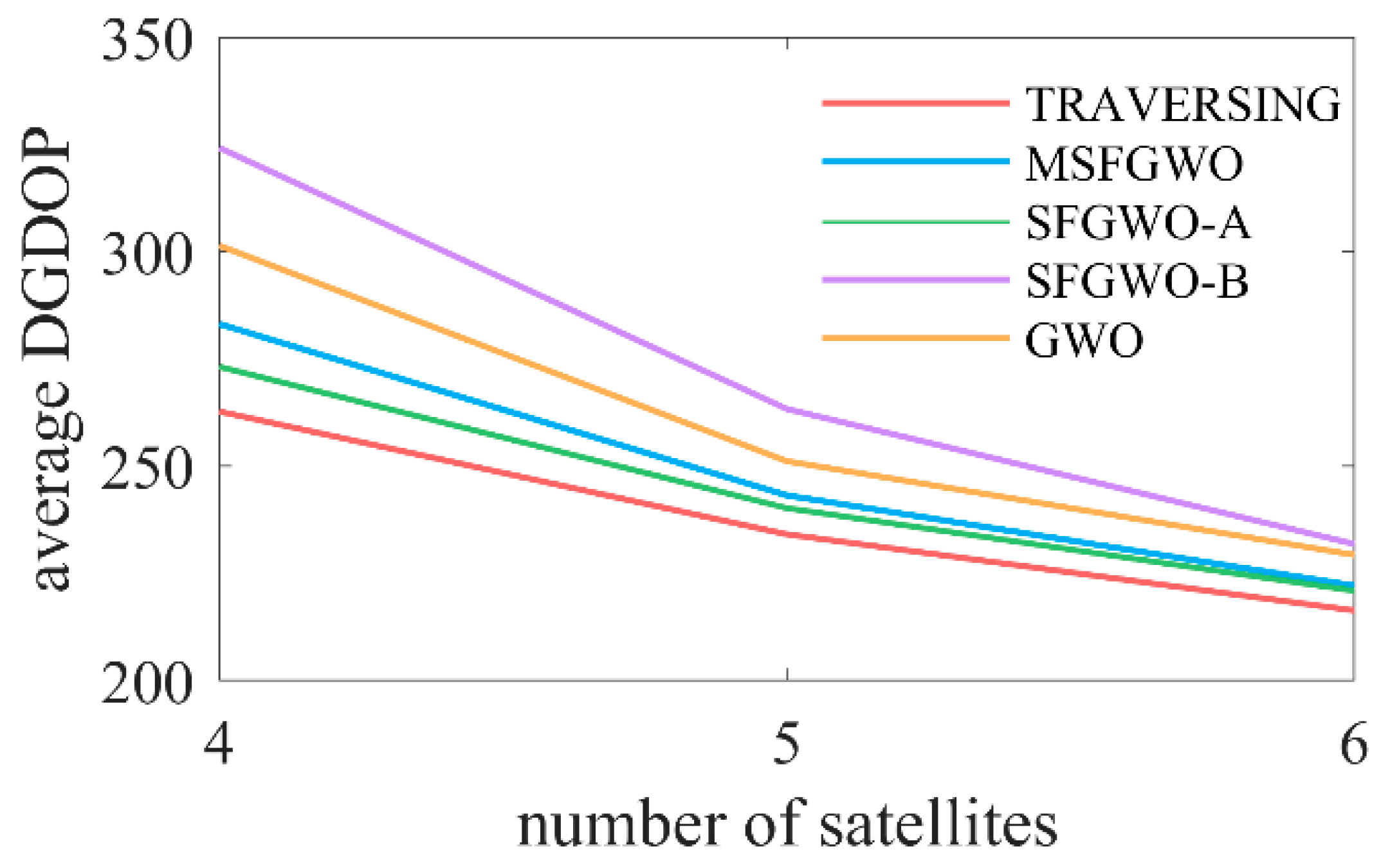
The reliability of the algorithms in the experiment was quantified by the ratio defined as the DGDOP value of a given algorithm divided by the DGDOP value obtained using the exhaustive search method. A lower ratio indicates that the DGDOP value of the selection result generated by an algorithm is closer to the optimal DGDOP value obtained through an exhaustive search; in particular, the associated results demonstrate the superior performance of the MSFGWO method. 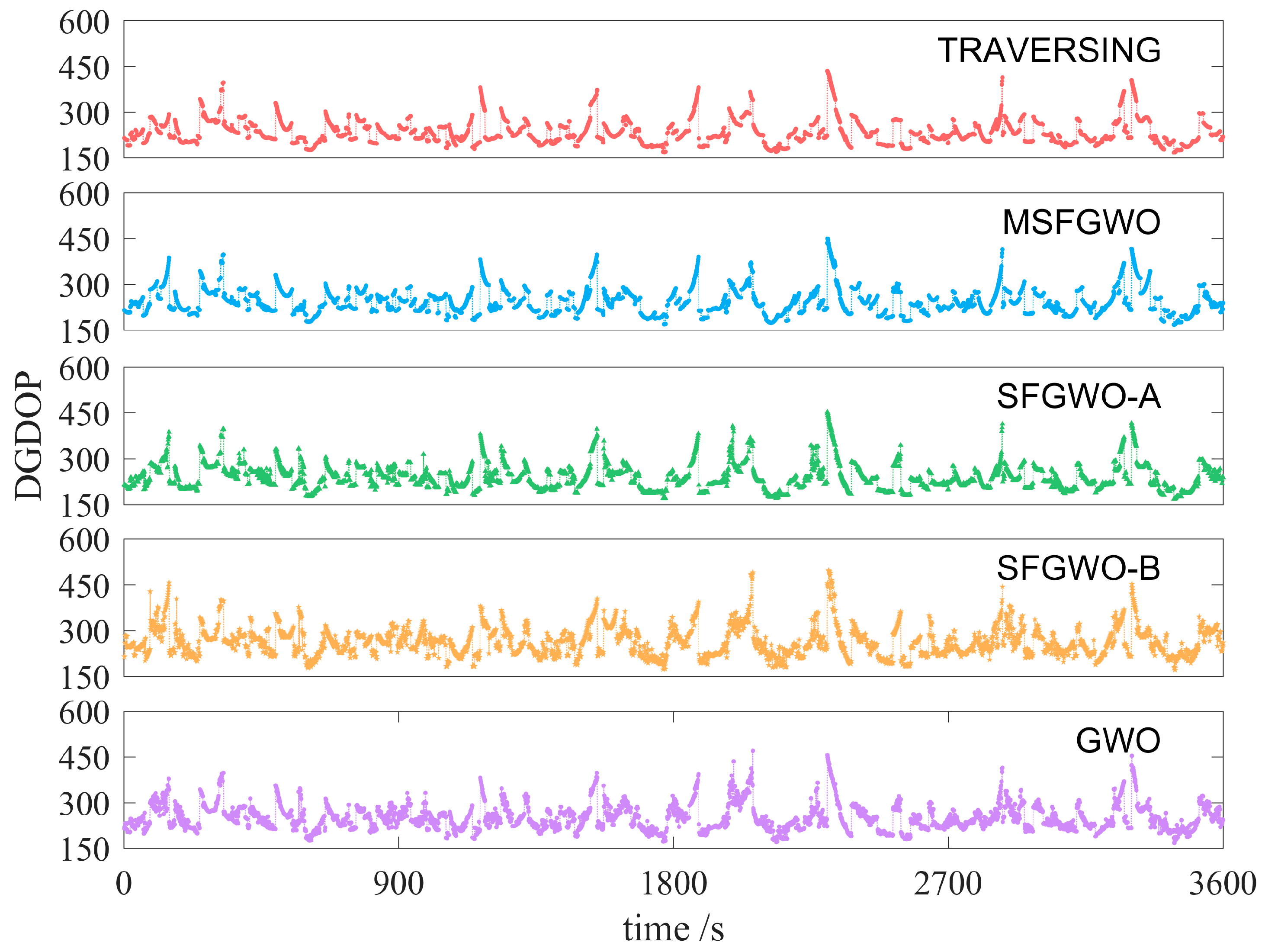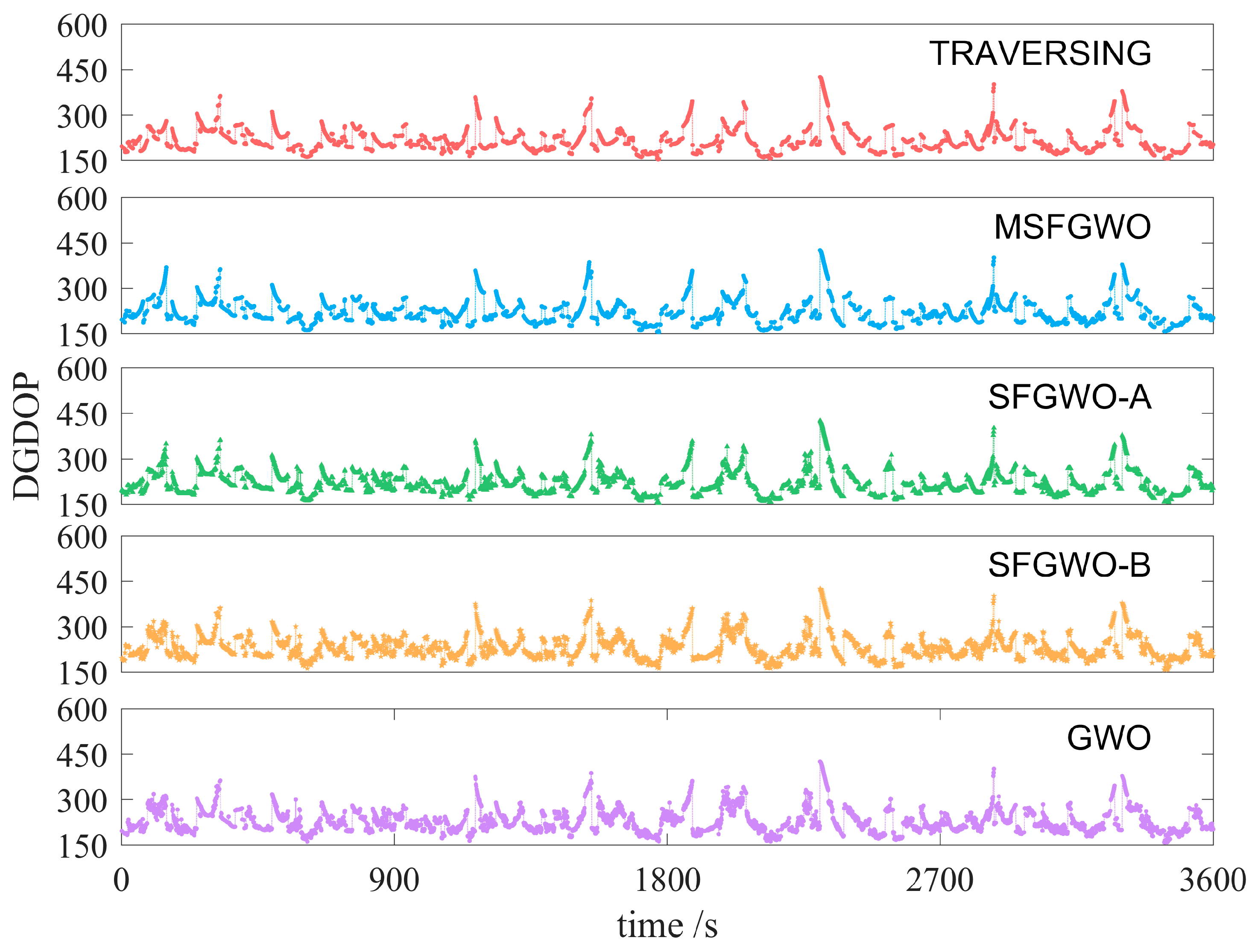Figure 9, Figure 10 and Figure 11 illustrate the DGDOP values of the satellite selection results per second for different algorithms selecting four, five, or six satellites, respectively. Figure 12 presents a comparison of the average DGDOP values, while Figure 13 compares the ratios of these average DGDOP values.

Based on analysis of the data presented in Figure 9, Figure 10, Figure 11, Figure 12 and Figure 13 and

Table 1. DGDOP values under different numbers of selected satellites.

	4 Satellites		5 Satellites		6 Satellites
	Average	Ratio	Average	Ratio	Average	Ratio
Traversal	262.71		234.06		216.28
GWO	301.39	1.15	251.11	1.07	229.27	1.06
SFGWO-A	273.14	1.04	240.16	1.03	220.88	1.02
SFGWO-B	324.21	1.24	263.29	1.13	231.79	1.07
MSFGWO	283.12	1.08	243.14	1.04	222.08	1.03

, it is evident that as the number of selected satellites increases, the DGDOP values calculated by each algorithm exhibit a consistent downward trend. Specifically, among the four algorithms, the DGDOP value obtained with the SFGWO-A was closest to that of the traversal method, with a ratio of 1.02 when selecting six satellites. This indicates that integrating the perturbation mechanism of the VNS algorithm and the mutation strategy of the GA into the GWO algorithm significantly enhances its global search capability for optimal solutions. In contrast, SFGWO-B aims to optimize the satellite continuous observation time through incorporating the EWM algorithm into the GWO algorithm. However, this approach resulted in a slight increase in DGDOP values in exchange for extended continuous observation times. Due to the tendency of the GWO algorithm to fall into local optima, the DGDOP value of SFGWO-B was higher than that of the standard GWO algorithm, representing the highest DGDOP value among the four algorithms. Conversely, the MSFGWO algorithm proposed in this study achieved a balance between optimizing the DGDOP value and ensuring continuous satellite observations. Consequently, its DGDOP value was lower than that of the traditional GWO algorithm and SFGWO-B but slightly higher than that of SFGWO-A and the traversal method. Additionally, the MSFGWO algorithm demonstrated relatively stable optimization performance, with a ratio of 1.03 when selecting six satellites, indicating that it effectively balances practical continuous observation requirements with higher accuracy.

The aforementioned experimental results substantiate that incorporating the perturbation mechanism of the VNS algorithm and the mutation strategy of the GA into the GWO algorithm significantly enhances the population diversity and effectively mitigates the risk of converging to local optima. This integration boosts the overall optimization capability of the GWO algorithm, thereby reducing the DGDOP value. However, the introduction of the EWM algorithm to optimize the continuous satellite observation time resulted in a marginal increase in the DGDOP value.

4.2. Analysis of Time Consumption

The computational time directly reflects the efficiency of a satellite selection algorithm, where a shorter computation time indicates a higher efficiency in satellite selection. Figure 14 illustrates the computational time per second for the different algorithms when selecting four, five, or six satellites. Figure 15 provides a comparison of the average computational time across different algorithms. Figure 16 presents the comparative analysis of the average difference in computational time between various algorithms and the exhaustive search method.

Table 2. Time consumption values under different numbers of selected satellites.

	4 Satellites		5 Satellites		6 Satellites
	Average (s)	Efficiency Improvement (%)	Average (s)	Efficiency Improvement (%)	Average (s)	Efficiency Improvement (%)
Traversal	0.0442		0.1110		0.2650
GWO	0.0088	80.09	0.0092	91.71	0.0106	96.00
SFGWO-A	0.0151	65.84	0.0164	85.23	0.0173	93.47
SFGWO-B	0.0089	79.86	0.0099	91.08	0.0108	95.92
MSFGWO	0.0162	63.35	0.0166	85.05	0.0174	93.43

summarizes the computational time for different algorithms and the time difference relative to the exhaustive search method, thereby offering a comprehensive evaluation of the performance of these algorithms in terms of their satellite selection efficiency.

Based on analysis of the data presented in Figure 14, Figure 15 and Figure 16 and Table 2, it is evident that as the number of selected satellites increases, the computational time required for each algorithm exhibits an upward trend. Specifically, the traversal method demonstrated significant fluctuations in computational time per second, whereas the intelligent optimization algorithms showed relatively minor variations. Moreover, the increase in computational time for the traversal method was markedly higher, when compared to the intelligent optimization algorithms, as the number of selected satellites increased. Notably, the GWO and SFGWO-B algorithms exhibited slightly lower computational times than the SFGWO-A and MSFGWO algorithms. This suggests that the incorporation of the VNS perturbation mechanism and the GA mutation strategy into the GWO algorithm increases its computational complexity, thereby leading to a longer computational time. The minimal difference in computational time between the GWO and SFGWO-B algorithms, as well as between the SFGWO-A and MSFGWO algorithms, indicates that the introduction of the EWM algorithm has a limited impact on computational time. Although the MSFGWO algorithm proposed in this study had the highest computational time among the four optimization algorithms, it remained significantly lower than that of the traversal method. For instance, when selecting six satellites, the MSFGWO algorithm consumed 0.0174 s, and the calculation efficiency is increased by 93.43% when compared to the traversal method.

In summary, the experimental results indicate that incorporating the perturbation mechanism of the VNS algorithm and the mutation strategy of the GA into the GWO algorithm leads to a slight increase in computational time; in contrast, integrating the EWM algorithm results in a relatively smaller increase in computational time. In both cases, the computational time remained significantly lower when compared to the traditional exhaustive search method.

4.3. Analysis of the Number of Satellite Switches Between Adjacent Moments

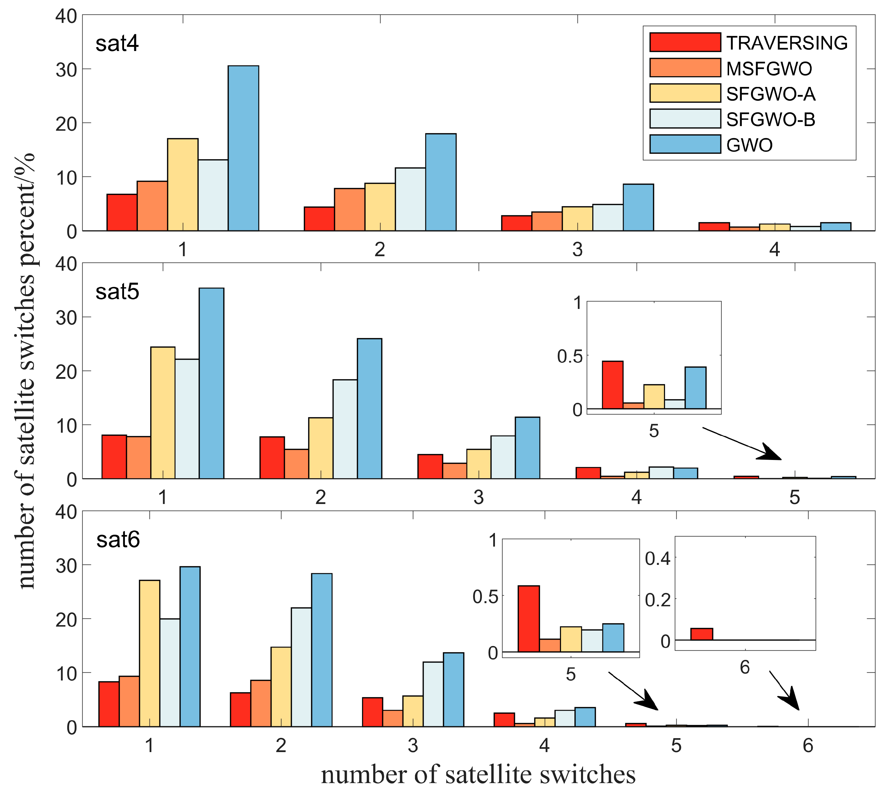
A reduced number of satellite switches between adjacent moments allows for prolonged continuous observation of the same group of satellites, thereby enhancing the accuracy and stability of positioning. Figure 17 illustrates the number of satellite switches between adjacent moments when selecting four, five, or six satellites, along with the percentage of these switching instances relative to the total observation duration.

Table 3. The number of satellite switches in adjacent moments when selecting four satellites.

Number of Satellite Switches	Traversal	GWO	SFGWO-A	SFGWO-B	MSFGWO
0	3046	1490	2465	2506	2837
1	242	1100	614	473	331
2	158	647	315	418	281
3	99	309	160	174	126
4	54	53	45	28	24

,

Table 4. The number of satellite switches in adjacent moments when selecting five satellites.

Number of Satellite Switches	Traversal	GWO	SFGWO-A	SFGWO-B	MSFGWO
0	2778	899	2069	1775	3003
1	292	1272	898	798	279
2	277	934	406	659	196
3	162	410	195	286	103
4	74	70	43	78	16
5	16	14	8	3	2

and

Table 5. The number of satellite switches in adjacent moments when selecting six satellites.

Number of Satellite Switches	Traversal	GWO	SFGWO-A	SFGWO-B	MSFGWO
0	2771	883	1822	15,744	2819
1	298	1066	976	718	337
2	225	1021	530	792	309
3	193	492	205	430	109
4	89	128	58	108	21
5	21	9	8	7	4
6	2	0	0	0	0

detail the specific number of satellite switches for different algorithms when four, five, or six satellites are selected, respectively.

Table 6. Longest continuous observation times under different numbers of selected satellites.

	4 Satellites	5 Satellites	6 Satellites
Traversal	31	37	22
GWO	21	23	21
SFGWO-A	43	25	22
SFGWO-B	51	38	21
MSFGWO	48	54	45

provides a comparison of the longest observable time across the different algorithms.

Based on analysis of the data presented in Figure 17 and Table 3, Table 4 and Table 5, it is evident that the GWO algorithm exhibited a higher frequency of satellite switching between adjacent time intervals, with a larger number of satellites being switched each time. In contrast, both the SFGWO-B and MSFGWO algorithms demonstrated lower switching frequencies and fewer satellite switches between adjacent moments. This indicates that incorporating the EWM algorithm into the GWO framework effectively reduces satellite switching, thereby enhancing the continuous observation time for the same group of satellites. However, due to issues such as reduced diversity and susceptibility to local optima in the SFGWO-B algorithm, despite the reduction in satellite switching achieved through the introduction of the EWM algorithm, significant switching still occurred as the global optimal solution remained difficult to attain. Although the traversal method could identify the optimal satellite combination, it does not account for the impact of satellite switching, resulting in a high number of satellite changes between adjacent moments. Notably, when selecting five or six satellites, the MSFGWO algorithm achieved zero satellite switches between adjacent moments, meaning that no simultaneous replacement of five or six satellites occurred. Table 6 further highlights the advantage of the MSFGWO algorithm in terms of the longest continuous visible time; specifically, when selecting six satellites, it achieved a continuous observation time of 45 s, which is twice the value of 22 s observed with the traversal method.

In summary, the experimental results demonstrate that the integration of the EWM algorithm into the GWO algorithm not only effectively reduces the frequency of satellite handovers between consecutive time intervals but also significantly prolongs the continuous observation duration for the same set of satellites. This enhancement contributes to improving the stability and reliability of positioning solutions.

4.4. Analysis of Algorithm Positioning Performance

The analysis of satellite positioning accuracy is carried out from two aspects: planar positioning accuracy (2D) and three-dimensional positioning accuracy (3D). Figure 18 presents a comparative analysis of the 2D and 3D positioning accuracy for various satellite selection algorithms when four, five, and six LEO satellites are selected.

Table 7. The 2D and 3D position accuracy values under different numbers of selected satellites.

	4 Satellites		5 Satellites		6 Satellites
	2D (m)	3D (m)	2D (m)	3D (m)	2D (m)	3D (m)
Traversal	152.05	239.93	132.88	209.91	119.82	189.36
GWO	156.51	253.12	135.19	216.77	120.87	195.79
SFGWO-A	152.92	239.89	131.68	211.46	119.46	189.73
SFGWO-B	157.95	261.86	138.32	222.21	123.31	196.42
MSFGWO	151.94	240.97	132.08	210.23	121.43	192.86

systematically summarizes the positioning accuracy comparisons of different satellite selection algorithms under the same conditions of selecting four, five, and six LEO satellites.

From the data analysis presented in Figure 18 and Table 7, it is evident that as the number of selected satellites increases, the positioning accuracy calculated by each algorithm exhibits a downward trend. The SFGWO-A algorithm demonstrates relatively superior positioning performance compared to the other three intelligent optimization algorithms, whereas the SFGWO-B algorithm exhibits relatively inferior positioning performance. This is because the SFGWO-A algorithm integrates the perturbation strategy of the VNS algorithm and the mutation strategy of the GA algorithm into the traditional GWO algorithm, thereby enhancing the global optimization capability of the algorithm. The SFGWO-B algorithm incorporates the EWM algorithm into the traditional GWO algorithm, trading a portion of positioning accuracy for an extended continuous observation time of satellites. It is evident that the trend of the positioning result closely resembles the trend of the DGDOP value. The MSFGWO algorithm not only enhances the positioning accuracy but also simultaneously extends the continuous observation time of the satellite combination. With the increase in the number of selected LEO satellites, the 3D positioning accuracy shows a downward trend: the traversal method improves from 239.93 m to 189.36 m, the MSFGWO algorithm improves from 240.97 m to 192.86 m, the GWO algorithm decreases from 253.12 m to 195.79 m, the SFGWO-A algorithm decreases from 239.89 m to 189.73 m, and the SFGWO-B algorithm decreases from 261.86 m to 196.42 m. When selecting six satellites, compared with the three-dimensional positioning accuracy of the traversal method, the positioning accuracy of the MSFGWO algorithm, the GWO algorithm, the SFGWO-A algorithm, and the SFGWO-B algorithm is 3.5 m, 6.43 m, 0.37 m, and 7.06 m lower, respectively.

The aforementioned experimental results demonstrate that incorporating the perturbation strategy of the VNS algorithm and the mutation strategy of the GA algorithm into the GWO algorithm can significantly enhance the positioning accuracy of the algorithm. However, upon the introduction of the EWM algorithm, a certain degree of positioning accuracy must be traded off to optimize the continuous observation time of satellites. In contrast, the MSFGWO algorithm demonstrates an effective ability to strike a balance between positioning accuracy and the continuous observation time of satellites.

5. Conclusions

This study introduced a satellite selection method utilizing the proposed MSFGWO, which is specifically tailored to address the unique characteristics of LEO satellites, including their high velocity and brief visibility periods. Through a series of simulation experiments, we evaluated the performance of various algorithms with respect to their DGDOP values, computational time consumption, and times of satellite switching at adjacent moments when selecting different numbers of satellites. The experimental results demonstrated that the perturbation mechanism of the VNS algorithm and the mutation strategy of the GA can substantially enhance the global search capability of the GWO algorithm, thereby leading to a significant reduction in the DGDOP value. Furthermore, through an analysis of the times of satellite switching at adjacent time intervals, it was confirmed that the integration of the EWM algorithm into the GWO algorithm can substantially reduce the frequency of satellite switching and extend the continuous observation duration for the same group of satellites. Specifically, when selecting six satellites, the MSFGWO algorithm yielded an average DGDOP value of 222.08. Compared with the DGDOP ratio of the traversal method, it is 1.03. The 3D positioning accuracy is 192.86 m, and the positioning error is improved by 54.43% compared with the positioning accuracy of the traditional GWO algorithm. Furthermore, the system achieved a continuous observation duration of up to 45 s, with zero instances of switching between the six satellites at adjacent time points. This significantly enhances the stability and reliability of the positioning solution. Despite having the shortest computational time, the GWO algorithm exhibited relatively inferior satellite selection performance. Conversely, although the introduction of multiple strategies into the MSFGWO algorithm led to a slight increase in its computational time, it remained significantly lower than that of the exhaustive search method; for example, when selecting six satellites, the MSFGWO algorithm consumed only 0.0174 s, and the calculation efficiency is increased by 93.43% when compared to the traversal method.

In summary, the MSFGWO algorithm introduced in this paper not only achieves an optimal balance between the DGDOP value and the satellite switching times between adjacent moments but also significantly enhances the satellite selection efficiency. This algorithm significantly enhances the overall optimization capabilities of the GWO algorithm, thus effectively reducing the DGDOP value, improving positioning accuracy, minimizing the satellite handover times between adjacent time intervals, and substantially extending the continuous observation duration for the same set of satellites. Consequently, the proposed method contributes to improvements in the stability and accuracy of positioning solutions.