KDFE: Robust KNN-Driven Fusion Estimator for LEO-SoOP Under Multi-Beam Phased-Array Dynamics

Abstract

Accurate Doppler frequency estimation for Low Earth Orbit (LEO)-based Signals of Opportunity (SoOP) positioning faces significant challenges from extreme dynamics (±40 kHz Doppler shift, 0.4 Hz/ms fluctuation) and severe SNR fluctuations induced by multi-beam switching. Empirical analysis reveals that phased-array beamforming generates three-tiered SNR fluctuation patterns during unpredictable beam handovers, rendering conventional single-algorithm solutions fundamentally inadequate. To address this limitation, we propose KDFE (KNN-Driven Fusion Estimator)—an adaptive framework integrating the Rife–Vincent algorithm and MLE via intelligent switching. Global FFT processing extracts real-time Doppler-SNR parameter pairs, while a KNN-based arbiter dynamically selects the optimal estimator by: (1) Projecting parameter pairs into historical performance space, (2) Identifying the accuracy-optimal algorithm for current beam conditions, and (3) Executing real-time switching to balance accuracy and robustness. This decision model overcomes the accuracy-robustness trade-off by matching algorithmic strengths to beam-specific dynamics, ensuring optimal performance during abrupt SNR transitions and high Doppler rates. Both simulations and field tests demonstrate KDFE’s dual superiority: Doppler estimation errors were reduced by 26.3% (vs. Rife–Vincent) and 67.9% (vs. MLE), and 3D positioning accuracy improved by 13.6% (vs. Rife–Vincent) and 49.7% (vs. MLE). The study establishes a pioneering framework for adaptive LEO-SoOP positioning, delivering a methodological breakthrough for LEO navigation.

1. Introduction

Global Navigation Satellite Systems (GNSS) are the cornerstone of modern positioning and timing infrastructure, with critical transport, industrial, and military applications [1]. However, their medium Earth orbit is a fundamental limitation. Signal path loss between GNSS satellites and terrestrial receivers typically ranges between −157 dB and −159 dB [2], rendering the systems unreliable in signal-degraded environments. For example, urban canyons, dense foliage areas, and indoor spaces frequently experience GNSS outages or suffer larger positioning errors because of the low residual power of the ground-reaching signal imposed by this path loss [3]. This strong limitation generates a strong demand for complementary positioning solutions.

In the field of navigation and positioning, signals of opportunity (SoOP) are signals not specifically designed for navigation and positioning but usable for this purpose. SoOP has emerged as a critical backup and extension of GNSS, with increasing research efforts dedicated to mitigating GNSS vulnerabilities [4]. Among modern wireless communication signals used for diverse applications—Wi-Fi networks [5], fifth-generation cellular networks for mobile phones [6], digital television [7], and amplitude modulation/frequency modulation radio broadcasting [8]—those transmitted by low Earth orbit (LEO) satellites are the most suitable as SoOP sources for opportunistic positioning applications [9]. Specifically, LEO-based SoOP provides markedly higher received power, allowing for faster resolution of positioning ambiguities—owing to their orbital characteristics that increase the number of possible geometric configurations—and providing increasingly global coverage through emerging megaconstellations [10]. Through these combined advantages, LEO–SoOP represents a particularly promising alternative to GNSS for accurate positioning in environments where GNSS signals are degraded or unavailable.

The extremely large Doppler shifts affecting LEO satellite signals explain why Doppler frequency analysis has become the main approach to LEO–SoOP positioning, which consists of deriving receiver coordinates from the joint processing of Doppler shifts, signal timestamps, and predicted ephemerides. Extensive scientific studies have demonstrated the feasibility of this approach for several constellations of LEO communication satellites. For example, in open-sky conditions, LEO–SoOP positioning with Iridium NEXT achieves a two-dimensional positioning root-mean-square error (RMSE) of less than 20 m [11]. For maritime tracking, ORBCOMM-based LEO–SoOP positioning achieves an accuracy of 50–200 m [12]. Additionally, Starlink-based LEO–SoOP positioning, through differential Doppler positioning techniques, achieves an accuracy of 33.4 m [13]. Moreover, recently developed multi-constellation data fusion techniques [14,15] have considerably reduced positioning errors relative to single-system methods.

Iridium NEXT, as an early representative of LEO satellite constellations, has been investigated intensively for scientific research on SoOP-based positioning. A distinctive feature of Iridium NEXT broadcasts is the inclusion of an unmodulated pilot signal (hereafter “tone signal”) in the broadcast channel at the start of each frame, with optimal characteristics for Doppler frequency estimation. Most previous studies used this tone signal to measure Doppler frequencies or to obtain coarse Doppler frequency estimates. Because the accuracy of the Doppler frequency estimate obtained from the tone signal directly determines the positioning accuracy, the frequency estimation algorithm is a critical component of the positioning process workflow. In 2021, a research group developed an innovative positioning framework that combined signals from Iridium NEXT and ORBCOMM [16]. Their method consisted of, first, applying frequency-domain scaling to the received signal, then extracting Doppler information using Fast Fourier Transform (FFT), and, finally, employing Kalman filtering for position determination. In 2020, another publication introduced a Doppler frequency estimation algorithm for weak-signal environments, which represented a notable improvement in Doppler frequency estimation from Iridium NEXT signals [17]. After a coarse initial estimation using FFT, the algorithm quadruples the estimated frequency to remove quadrature phase-shift keying (QPSK) modulation artifacts before applying maximum likelihood estimation (MLE) to refine the Doppler frequency estimate. In 2022, the same research group implemented two important algorithm updates [18]. First, they combined data from the Iridium NEXT tone signal and ORBCOMM signals, considerably improving their algorithm’s achieved accuracy, with a two-dimensional positioning RMSE of 59.7 m [18]. Second, they implemented an innovative “phase–time method” comprising a two-stage estimation process: the Iridium tone signal is first processed through FFT and MLE before down-conversion and comprehensive MLE analysis of the complete-frame signal, resulting in enhanced stability and reliability [19]. Slightly earlier, in 2020, a research group from Tsinghua University in Beijing, China, had developed a method leveraging both the explicit and implicit Iridium tone signals [20] by first estimating the Doppler frequency from each tone component by FFT and applying the compensation algorithm of Rife and Vincent [21] (hereafter “Rife–Vincent algorithm”) and then obtaining the final Doppler frequency estimate by fusing the explicit and implicit tone signals, thereby improving estimation accuracy.

The Iridium NEXT tone signal intrinsically presents notable processing challenges. Its very short duration (T = 2.56 ms) fundamentally complicates FFT-based Doppler frequency estimation, limiting the maximum spectral resolution to 390 Hz (1/T). This coarse resolution introduces substantial estimation errors that propagate directly to the positioning accuracy. Although existing methods generally use FFT to produce a preliminary coarse estimation, subsequently refined with MLE or Rife–Vincent algorithms, they are critically limited for effective processing of real Iridium NEXT signals. First, the beam switching and other behaviors of Iridium-phased array antennas have led to severe SNR fluctuations [22,23]. The substantial interframe signal-to-noise ratio (SNR) variations severely affect algorithm robustness [24], notably because MLE, nominally an optimal estimation method, exhibits unstable performance for moderately low SNR. Although previous research has statistically analyzed the SNR variation of Iridium satellites [24], there has been no systematic analysis and research on the mechanism of these variations. Second, the Rife–Vincent algorithm is particularly sensitive to the strong Doppler frequency variability between frames (within a range of ±40 kHz [25]): compensation accuracy drastically degrades when the Doppler frequency is close to a spectral line in the FFT spectrum [26], causing complete algorithm failure in numerous practical scenarios. These challenges create a strong research gap because existing standard solutions cannot provide reliable frequency estimation for the full operational envelope of Iridium NEXT signals. Although numerous prior studies have optimized frequency estimation under severe SNR fluctuations [27,28], they neither embedded these solutions within the specific context of LEO SoOP Doppler frequency estimation nor validated their algorithmic efficacy in this scenario. Therefore, a robust estimation algorithm is urgently required to simultaneously alleviate frequency resolution constraints imposed by short-duration tone signals, performance reliability problems under fluctuating SNR conditions, and accuracy inconsistencies across the operational range of Doppler frequency variations.

To account for these fundamental limitations, we propose a novel KNN-Driven Fusion Estimator (KDFE) for Doppler frequency estimation from SoOP, which is an original Doppler frequency estimation algorithm relying on Iridium NEXT signals and combining the advantages of the Rife–Vincent and MLE algorithms through simultaneous optimization of two constraining parameters: the SNR, which characterizes signal quality, and the frequency offset factor, which characterizes the frequency difference between the FFT peak (FFT spectral line with maximum amplitude) and the true signal. The proposed algorithm introduces three key innovations:

• Frame synchronization of Iridium SoOP (by using prior information); signal frames are accurately divided to obtain more accurate parameter estimates;
• Systematic organization and analysis of the SNR fluctuations between Iridium satellites, beams, and intra-beams;
• An adaptive KNN-based decision mechanism to automatically select the optimal processing path on the basis of the real-time Iridium NEXT signal conditions, especially for small frequency offset factors, when the Rife–Vincent compensation performance degrades considerably;

The remainder of the manuscript is organized as follows: Section 2 describes the Iridium NEXT signal properties and the challenges in SoOP positioning; Section 3 presents the proposed KDFE algorithm; Section 4 and Section 5 describe the simulation and experimental results, respectively; and Section 6 provides a brief conclusion.

2. Iridium NEXT Signal Characteristics

2.1. Iridium NEXT Frame Structure

The Iridium NEXT system employs a discontinuous signal structure and hybrid time division multiple access and frequency division multiple access modulation schemes for frame transmission [29]. The frequency-domain system architecture comprises two distinct communication channels in the L-band: a simplex channel for downlink transmission from satellite to ground—from 1626.020833 to 1626.479167 MHz frequency range—and a duplex channel—1616–1626 MHz frequency range—for bidirectional satellite–ground communication (Figure 1). The simplex channel is partitioned into 12 sub-bands with identical bandwidth (41.667 kHz) and center frequencies defined as 1626.020833 MHz + n × 41.667 kHz, where n represents the sub-band index (0 ≤ n ≤ 11). The duplex channel is partitioned into 30 sub-bands with identical bandwidth (333.33 kHz), each containing eight frequency access points with individual bandwidths of 31.5 kHz and center frequency spacing of 41.667 kHz (Figure 1).

Similarly, the time–domain structure of the Iridium NEXT signal frame (duration: 90 ms) is well-defined, divided into simplex and duplex channels (Figure 2). The simplex channel duration is 20.32 ms, with three sequential components: an unmodulated tone, a binary phase shift keying-modulated unique word, and a QPSK-encoded data segment, with durations of 2.56 ms, 0.48 ms, and 17.48 ms, respectively [30]. The duplex channel occupies the remaining 69.68 ms, organized into eight slots of identical duration (8.28 ms) separated by guard times for bidirectional communication (Figure 2). The simplex channel is characterized by a regular transmission pattern and higher signal power than the duplex channel. Thus, it is suitable for SoOP positioning. Moreover, the lead component (tone) is an unmodulated, spectrally pure single carrier with constant envelope; hence, it is highly suitable for precise Doppler frequency estimation. Therefore, the primary objective of the proposed KDFE algorithm is to accurately estimate the Doppler frequency of the simplex channel tone signal, a critical but very short signal component.

2.2. Iridium NEXT Doppler Characteristics

As detailed in the previous sections, since the Iridium NEXT system employs a pilot signal (tone), it is particularly suitable for high-accuracy Doppler frequency estimation in SoOP positioning. However, the large Doppler variation range and substantial SNR fluctuations within and between Iridium NEXT signal frames introduce significant errors in Doppler frequency estimation, severely degrading the SoOP positioning accuracy.

The Iridium NEXT satellites are placed in LEO, characterized by a high orbital velocity and low altitude that induce high Doppler frequency variations—up to ±40 kHz—throughout an observation period [31]. This variation range (Figure 3) depends on the maximum elevation of each Iridium orbital plane. Such a wide range of Doppler variations not only requires the Doppler frequency estimation algorithms to possess extensive frequency acquisition capabilities but also generates serious technical difficulties. For example, the accuracy of the Rife–Vincent compensation algorithm decreases sharply for small-frequency offset factors (<0.15) [25], while more traditional phase-locked loops or Kalman filters with fixed step sizes might fail to track sudden frequency variations, resulting in the loss of lock [32].

2.3. Iridium NEXT SNR Characteristics

The SNR of Iridium downlinks is fundamentally governed by satellite antenna architecture. The operational Iridium NEXT constellation (

Table 1. Deployment of Iridium NEXT System.

Satellite Category	Plane 1	Plane 2	Plane 3	Plane 4	Plane 5	Plane 6
First-generation	0	0	6	0	0	0
Iridium NEXT	11	11	5	11	11	11

), progressively deployed since 2017, primarily comprises satellites equipped with L-band multi-beam phased array antennas (48 user beams per satellite via 3 phased arrays) implementing dynamic beamforming. However, this beam adaptability introduces spatiotemporal SNR variations across coverage areas due to rapid beam switching, posing critical challenges for signal synchronization.

There is a phased array antenna made up of three panels aboard each first-generation Iridium satellite [33,34]. However, in Iridium NEXT, the functionality of the three primary mission antennas is implemented by a main phased array antenna (Figure 4A). As illustrated in Figure 4B, the Iridium NEXT satellite employs a 12 × 10 uniform rectangular array (URA) as its main mission antenna (MMA), with overall dimensions of 924.572 mm × 1109.486 mm. The inter-element spacing is 92.457 mm in both the horizontal and vertical directions. The MMA generates 48 independent beams to serve users in different coverage directions of the Iridium satellite (Figure 5). The Iridium system sequentially polls all 48 beams every 4.32 s, with each beam allocated a 90 ms dwell time. Consequently, during Iridium signal observations, multiple factors—including inter-satellite variations, inter-beam discrepancies, and intra-beam fluctuations—can induce significant SNR variations. These SNR dynamics adversely affect the accuracy and robustness of parameter estimation, ultimately degrading positioning performance.

As an illustration, we conducted a statistical analysis of 1779 tones acquired by 8 Iridium satellites over a period of 30 min, which were received by a JCYX008 Iridium NEXT antenna. The statistical results of all of the 8 satellites indicate SNR values between −14 dB and 3 dB with a mean value of −6.33 dB, as illustrated in Figure 6. Figure 7 presents the frame-by-frame SNR distribution classified by satellite. These results show that the SNR of the Iridium tone fluctuates violently among different satellites due to the different orbits and states of each satellite.

Iridium satellites poll through 48 beams every 4.32 s to serve ground users at different azimuth and elevation angles. Therefore, due to frequent beam switching, signals originating from the same Iridium satellite still exhibit significant SNR fluctuations over short time intervals. Figure 8 illustrates beam switching and provides the corresponding SNR values for the Iridium 140 satellite, which confirm considerable SNR variations—up to 14 dB—between different beams. Even the tones from the same beam of the same satellite show up to 12 dB SNR fluctuation due to the different azimuth and elevation angles.

We also analyzed the acquisition time, beam, and SNR of each Iridium frame during the complete observation period of the Iridium 140 satellite, as shown in Figure 9. The satellite began being captured at the 14.38 min mark of the experiment until the last frame was acquired at 24.17 min, resulting in approximately 10 min of observation with 322 Iridium frames captured. We observed typical Iridium beam switching behavior. For instance, the coverage area of Group 6 beams is centered directly beneath the satellite, so frames from these beams were only captured during the middle segment of the observation period (i.e., when the satellite was at zenith). We observed two distinct patterns of SNR variation. First, during Iridium beam handovers, the receiver undergoes an instantaneous transition from the main lobe coverage of one beam to the side lobe region of another beam (Figure 10A), resulting in abrupt SNR fluctuations. This characteristic SNR variation pattern is observable at the 16.5 min mark in Figure 9, with instantaneous SNR variations reaching up to 7 dB. Second, during continuous reception from the same beam, the relative position between the receiver and the beam center evolves continuously. The beam edge exhibits a gradual power variation gradient (Figure 10B), leading to slow but persistent SNR changes. This SNR variation pattern is clearly visible at the 22 min mark in Figure 9 (indicated by the green diamond marker for beam identification). As the satellite moved, the beam’s coverage area shifted from directly illuminating the receiver (center) to marginal alignment (edge).

The detailed analysis of Iridium SNR variations reveals that the observed SNR fluctuations between different Iridium frames can be categorized into the following three patterns:

• SNR differences between distinct satellites: Variations caused by disparities in signal strength from different Iridium satellites.
• Instantaneous SNR fluctuations during beam handovers: Abrupt changes occur when the satellite beam handovers.
• Gradual SNR variations within the same beam: Slow changes due to the relative motion between the beam and receiver, affecting signal quality as the receiver moves from the beam center toward the edge.

In practical implementations, single-satellite data is processed independently for each signal channel, necessitating adaptive Doppler frequency estimation algorithms with robust performance under dynamic signal conditions to account for these SNR fluctuations.

3. The KDFE Algorithm

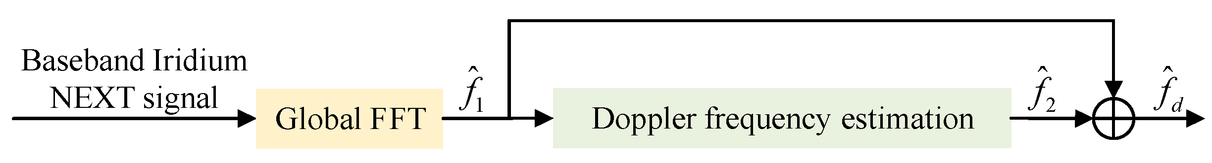
3.1. Existing Methods

Conventional Doppler frequency estimation algorithms typically apply global FF’T to SoOP to obtain a coarse preliminary estimate (${\widehat{f}}_1$), reprocessing this estimate with parametric refinement algorithms to compensate spectral leakage in the FFT results (${\widehat{f}}_2$), as illustrated in Figure 11. The Rife–Vincent algorithm and MLE method are the most widely used in this latter step because of their balanced computational efficiency.

The Rife–Vincent algorithm first determines the direction (sign) of the necessary frequency compensation from spectral lines adjacent to the FFT peak, as in Equation (1), and then calculates its magnitude using Equation (2) [21]:

$$a=\left\{\begin{array}{cc}1,& \left|X\left(k_0+1\right)\right|>\left|X\left(k_0-1\right)\right|\\ -1,& \left|X\left(k_0+1\right)\right|\le \left|X\left(k_0-1\right)\right|\end{array}\right.$$

(1)

$${\widehat{f}}_{Rife}={\displaystyle \frac{f_s}{N_{FFT}}}\cdot \left(k_0+{\displaystyle \frac{a\cdot \left|X\left(k_0+a\right)\right|}{\left|X\left(k_0+a\right)\right|+\left|X\left(k_0\right)\right|}}\right)\triangleq {\displaystyle \frac{f_s}{N_{FFT}}}\cdot \left(k_0+a\cdot \delta \right)$$

(2)

$$\delta \triangleq {\displaystyle \frac{\left|X\left(k_0+a\right)\right|}{\left|X\left(k_0+a\right)\right|+\left|X\left(k_0\right)\right|}}$$

(3)

where a is the Rife–Vincent compensation direction, $X\left(k\right)$ is the result of $N_{FFT}$-point FFT, $k_0$ is the index of the FFT peak (spectral line with maximum $\left|X\left(k\right)\right|$ value), $f_s$ is the sampling frequency, and $\delta \in \left[0,0.5\right]$ is the frequency offset factor previously mentioned, which characterizes the frequency difference between the FFT peak and the true signal.

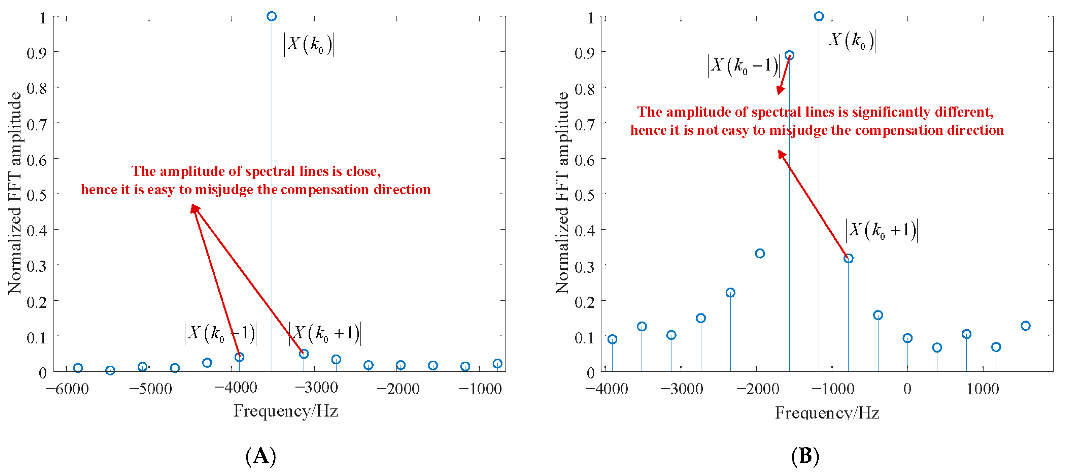
Substantial Doppler frequency variations in the Iridium NEXT system modify the frequency offset factor δ unpredictably, with strong performance degradation of the Rife–Vincent algorithm for small values. If the true signal frequency is nearly equal to that of an FFT sampling point, δ is small, and the $\left|X\left(k_0\pm 1\right)\right|$ values are considerably smaller than $\left|X\left(k_0\right)\right|$ but approximately equal to each other (Figure 12A). Under such conditions, noise interference can cause directional frequency compensation errors that strongly reduce the Doppler frequency estimation accuracy. Conversely, if the true signal frequency is approximately equidistant from adjacent FFT sampling points, δ is larger, and one of the $\left|X\left(k_0\pm 1\right)\right|$ values are comparable with $\left|X\left(k_0\right)\right|$ but markedly larger than the other (Figure 12B). Under such conditions, the probability of directional errors in the Rife–Vincent compensation markedly decreases, and the estimation accuracy remains excellent.

The theoretical RMSE of the Rife–Vincent algorithm with different δ can be expressed as:

$${\sigma }_{\mathrm{Rifle}}={\displaystyle \frac{f_s^2}{N^2}}\left\{{\displaystyle \frac{{\left(1-\left|\delta \right|\right)}^2\left[{\left(1-\left|\delta \right|\right)}^2+{\delta }^2\right]}{N\cdot {\sin \mathrm{c}}^2\left(\delta \right)\cdot SNR}}+2{\delta }^2\mathrm{erfc}\left[{\displaystyle \frac{\delta \left|\sin \left(\pi \delta \right)\right|}{\pi \left(1-{\delta }^2\right)}}\cdot \sqrt{N\cdot SNR}\right]\right\}$$

(4)

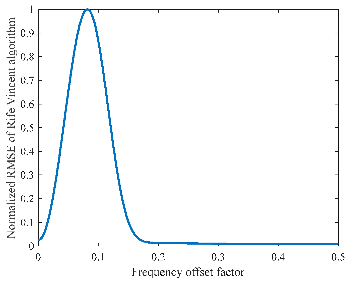
where $f_s$, $N$, and $SNR$ are the sampling frequency, number of FFT points, and SNR. Figure 13 demonstrates the normalized RMSE of the Rife–Vincent algorithm as a function of δ (at SNR = 0 dB). Performance degrades when δ assumes smaller values.

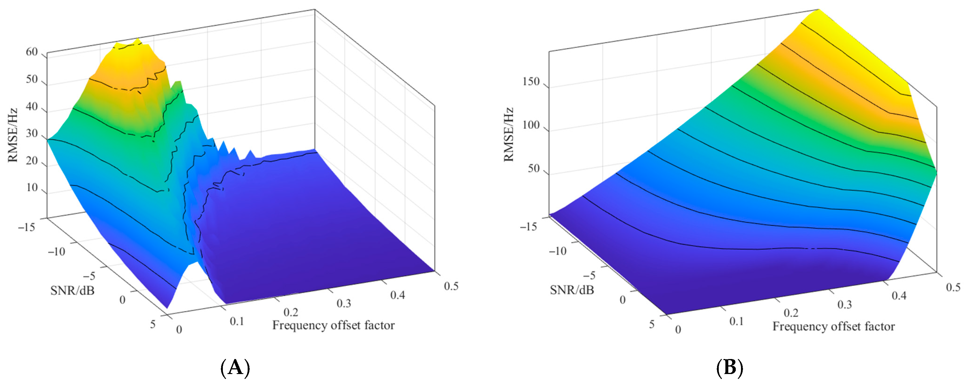
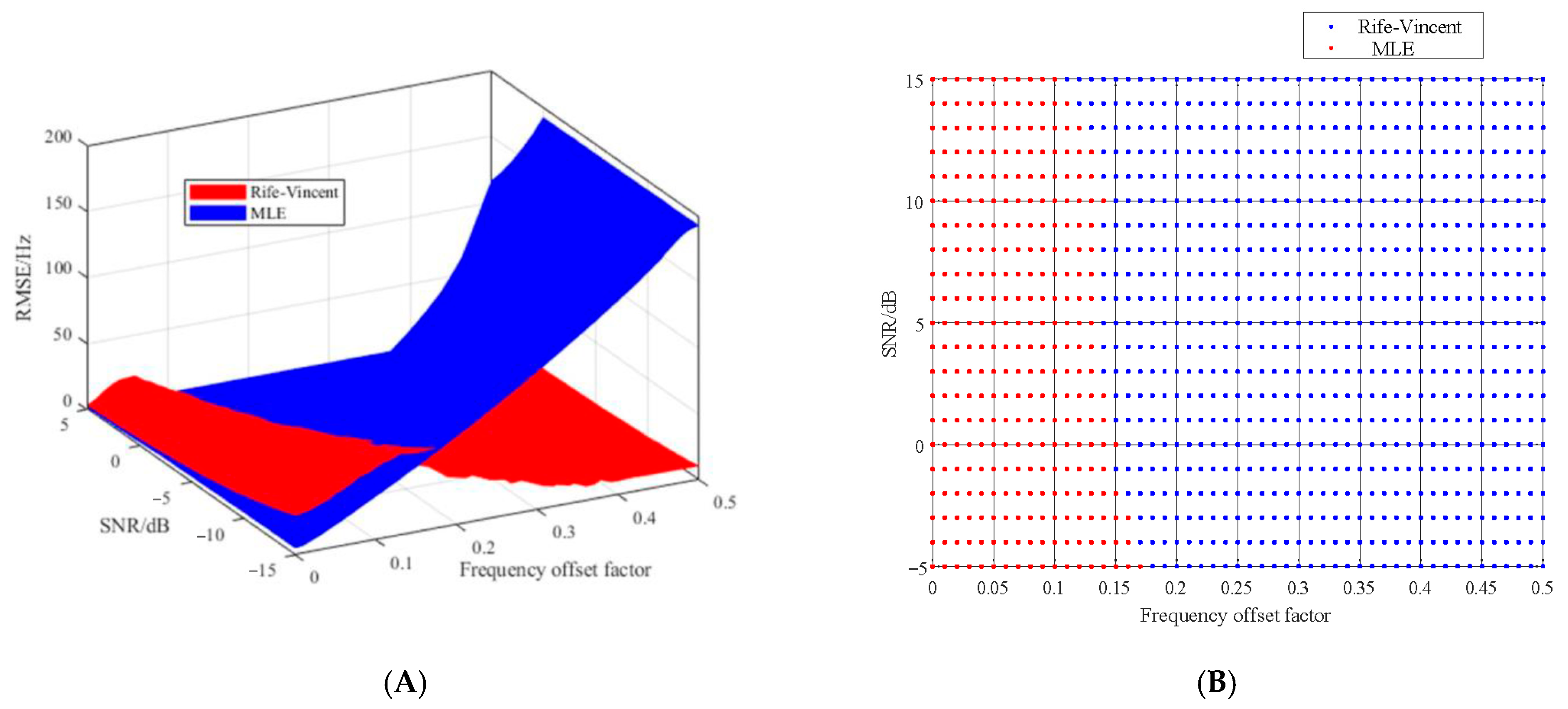
Figure 14A illustrates the sharp decrease in the Rife–Vincent algorithm accuracy (sharp RMSE increase) for small δ values, which is particularly large at low SNR. This dual dependence on δ and on the SNR defines the fundamental limitation of the Rife–Vincent algorithm for precise Doppler frequency estimation.

The MLE function is an unbiased estimator relying on the minimum RMSE of sampled points; its estimation accuracy strongly depends on sample quality. Consequently, MLE performance is highly sensitive to SNR fluctuations, exhibiting a sharp accuracy decrease under low-SNR conditions. Notably, because the MLE algorithm is a search-based method applied to the global FFT results, its performance also depends on the FFT estimation accuracy (Figure 14B). For small δ values, the FFT itself achieves high estimation accuracy, ensuring robust MLE performance despite large SNR variations. Hence, because of the complementarity of their optimal applicability domains, combining the Rife–Vincent and MLE algorithms can provide comprehensive coverage of most Iridium NEXT operational conditions and mitigate the effects inherent to LEO satellite signals of both SNR fluctuations and Doppler frequency variations on SoOP positioning.

3.2. New Algorithm Proposal

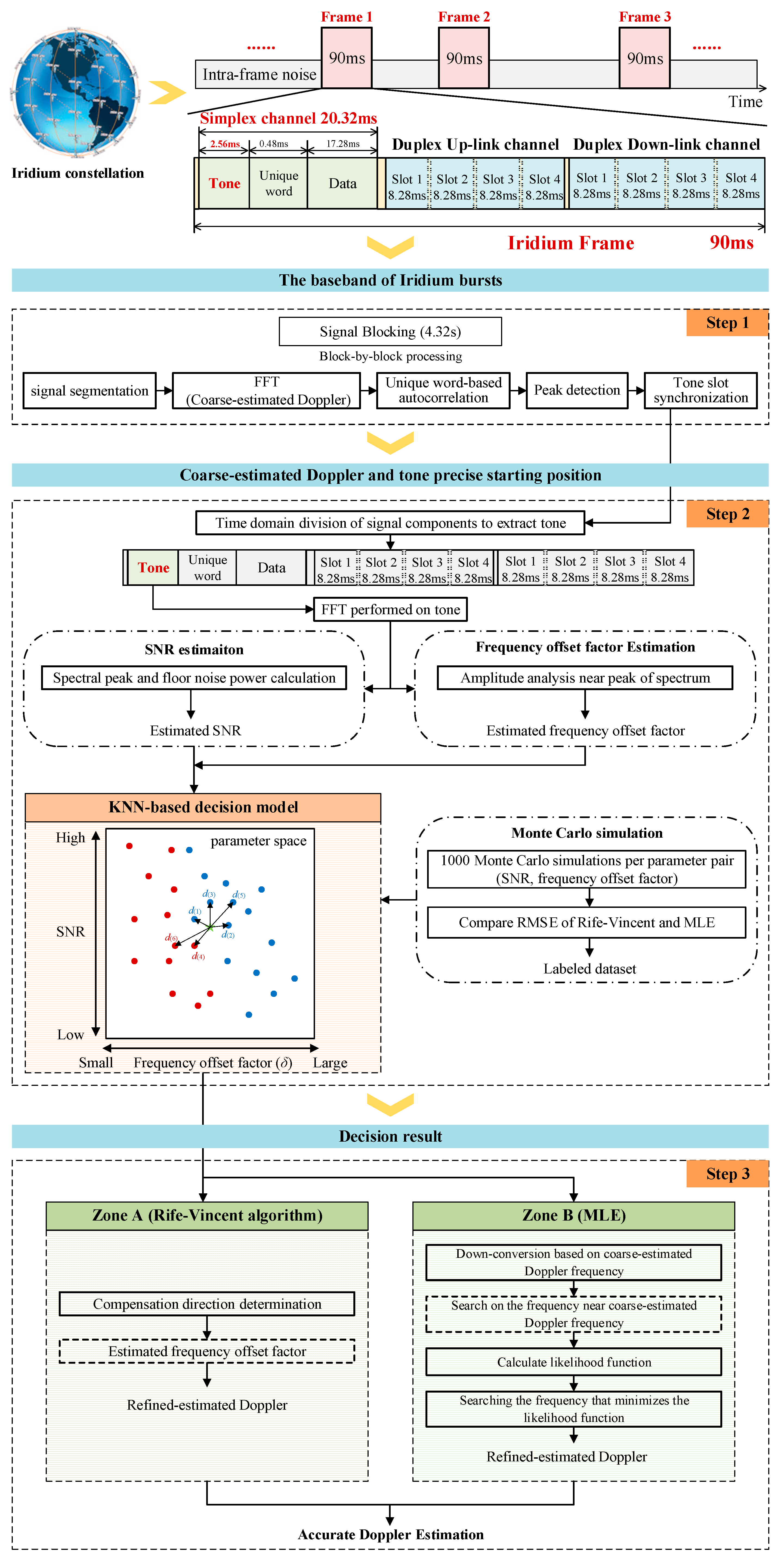
In this study, we propose a new algorithm, KDFE, for precise Doppler frequency estimation from Iridium NEXT tone signals. It consists of accounting for the SNR and δ characteristics of individual Iridium NEXT tone signals through adaptive integration of the Rife–Vincent and MLE algorithms. By adaptively selecting a processing path optimally suited for each Iridium NEXT tone signal, the KDFE algorithm can achieve higher Doppler frequency estimation accuracy than existing methods. The KDFE algorithm architecture, illustrated in Figure 15, includes three processing steps for each block. First, it performs a global FFT to determine the approximate position of Iridium frames, obtain a coarse Doppler frequency estimate (${\widehat{f}}_1^r$), and precisely locate the Iridium tone signals. Second, two characteristic parameters are extracted: frequency offset factor and SNR. The KNN-based decision module selects the optimal fine Doppler frequency compensation algorithm based on these parameters. Third, the decision result is applied to compensate (${\widehat{f}}_2^r$) for the coarse estimated Doppler frequency (${\widehat{f}}_1^r$) using FFT, and the refined Doppler frequency estimation (${\widehat{f}}_d^1$) is obtained.

In the first step, a global FFT is applied to the Iridium NEXT data. Because SoOP positioning requires a substantial volume of data acquired over long periods, an Iridium NEXT signal from the carrier wave has been removed (i.e., baseband signal). $x\left[n\right]$ can be expressed as some shorter, equal-duration blocks: ${\widehat{f}}_1$

$$x\left[n\right]={\displaystyle \sum _{i=0}^{N_{block}-1}{x}_{block,i}\left[n-B_i\right]}$$

(5)

where n is the index of the sampling points, $N_{block}$ is the total number of blocks in the analyzed signal, and $x_{block,i}$ and $B_i$ are the signal and starting point for block i, respectively. In subsequent processing steps, each block will serve as a standardized processing unit, undergoing independent computational operations to extract the corresponding observational parameters.

Because Iridium signals are discontinuous, the block is segmented into multiple segments, with each segment undergoing individual FFT processing (i.e., global FFT). Then the coarse location of the tone signal can be detected by analyzing the power output. Signal power for FFT segment j in a block can be calculated as:

$$P\left(j\right)=10\cdot \log \left({\displaystyle \frac{{\left|\max \left(X_j\left(k\right)\right)\right|}^2}{\frac{1}{M}{\displaystyle \sum _{j=1}^M{\left|\max \left(X_j\left(k\right)\right)\right|}^2}}}\right)$$

(6)

where M is the total number of FFT segments in the processed block. The location and length of each tone signal within the block can be obtained by determining the $P\left(j\right)$ peak positions in the block. Then, the signal for this block can be expressed as:

$$s_{block}\left[n\right]=s^1\left[n-N_1\right]+s^2\left[n-N_2\right]+\cdot \cdot \cdot +s^R\left[n-N_R\right]+{\epsilon }_s\left[n\right]$$

(7)

where $s^r$ and $N_r$ denote the r-th frame and its coarse starting time in the block, and ${\epsilon }_s\left[n\right]$ is the complex Gaussian white noise. As Equation (6) establishes, global FFT effectively separates frame signals from noise within each block of an Iridium NEXT baseband signal and provides preliminary Doppler frequency estimates (${\widehat{f}}_1^r$) for all individual frames.

We compute the precise starting sampling point for each tone based on the estimated coarse positions of Iridium frames obtained from the previous step. Using the frame’s starting sample point as the reference (i.e., the tone’s starting sampling point), the expression of the r-th frame can be written as:

$$s^r\left[n\right]=\left\{\begin{array}{c}{s}_{tone}\left[n\right];N_{frame}^r\le n\le N_{tone}^r\\ s_{uni}\left[n\right];N_{tone}^r<n\le N_{uni}^r\\ s_{data}\left[n\right];N_{uni}^r<n\le N_{data}^r\end{array}\right.$$

(8)

where $N_{frame}^r$ denotes the starting point of the r-th frame. $N_{tone}^r$, $N_{uni}^r$, and $N_{data}^r$ denote the sample points marking the end of the tone, unique word, and data portion, respectively. $s_{tone}\left[n\right]$, $s_{uni}\left[n\right]$, and $s_{data}\left[n\right]$ denote the tone, unique word, and data portion of the r-th frame, respectively. The $s_{tone}\left[n\right]$ is an unmodulated signal, which can be written as:

$$s_{tone}\left(t\right)=A_{tone}\cdot \exp \left(j\left(2\pi {\displaystyle \frac{f_d}{f_s}}n+{\phi }_{0,tone}\right)\right)+{\epsilon }_s\left(n\right)$$

(9)

where $A_{tone}$ and ${\phi }_{0,tone}$ denote the amplitude and initial phase of the tone. $f_s$ denotes the sampling frequency. The $s_{uni}\left[n\right]$ is modulated by BPSK, which can be written as:

$$s_{uni}\left(t\right)=A_{uni}\cdot \exp \left(j\left(2\pi {\displaystyle \frac{f_d}{f_s}}n+{\phi }_{0,uni}+\pi \cdot c_{uni}\left(⌈{\displaystyle \frac{n}{N_{symbol}}}⌉\right)\right)\right)+{\epsilon }_s\left(n\right)$$

(10)

where $A_{uni}$ and ${\phi }_{0,uni}$ denote the amplitude and initial phase of a unique word portion. $N_{symbol}$ represents the number of sampling points per symbol. $c_{uni}$ is the vector of binary information code of a unique word, which is prior information that can be shown as:

$$c_{uni}={\left(789\right)}_{\mathrm{H}}=\left[0 1 1 1 1 0 0 0 1 0 0 1\right]$$

(11)

The $s_{data}\left[n\right]$ is modulated by QPSK, which can be written as:

$$\begin{array}{l}{s}_{data}\left(n\right)=A_{data}\cos \left(2\pi {\displaystyle \frac{f_d}{f_s}}n+{\phi }_{0,data}+\pi \cdot c_{data,I}\left(⌈{\displaystyle \frac{n}{N_{symbol}}}⌉\right)\right)\\ =\mathrm{j}\cdot A_{data}\sin \left(2\pi {\displaystyle \frac{f_d}{f_s}}n+{\phi }_{0,data}+\pi \cdot c_{data,Q}\left(⌈{\displaystyle \frac{n}{N_{symbol}}}⌉\right)\right)+{\epsilon }_s\left(n\right)\end{array}$$

(12)

where $A_{data}$ and ${\phi }_{0,data}$ denote the amplitude and initial phase of a unique word portion. $c_{data,I}$ and $c_{data,Q}$ are the vector of binary information code of I and Q.

Since the tone and unique word are the prior information, a signal containing both tone and unique word portions can be generated and sampled according to the sampling frequency. Then, calculating the cross-correlation function between the generated signal $s_{gen}\left[n\right]$ and the frame signal, the point where the cross-correlation function reaches its maximum corresponds to the starting sample point of the tone. The starting sample point of the r-th tone in a block can be calculated using the following equation:

$$N_{tone}^r=\underset{k}{\arg }\max \left[R\left[k\right]\right]=\underset{k}{\arg }\max \left[{\displaystyle \frac{1}{N_{gen}}}{\displaystyle \sum _{n=1}^{N_{gen}}{s}^r\left[n-k\right]}\cdot s_{gen}\left[n\right]\right]$$

(13)

where $R\left[k\right]$ denotes the cross-correlation function between the generated signal $s_{gen}\left[n\right]$ and the frame signal $s^r\left[n\right]$, and $N_{gen}$ denotes the number of sampling points of $s_{gen}\left[n\right]$.

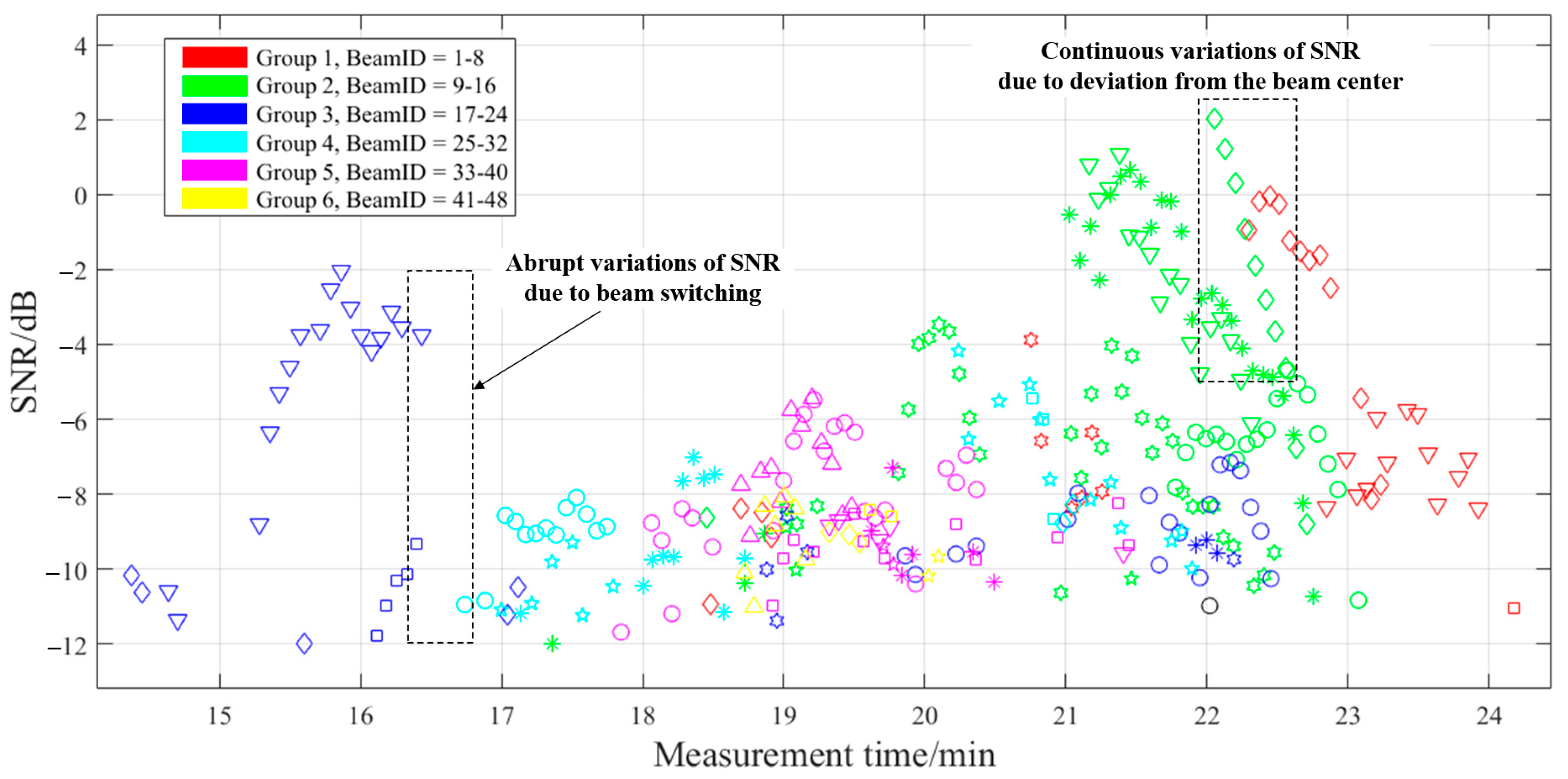
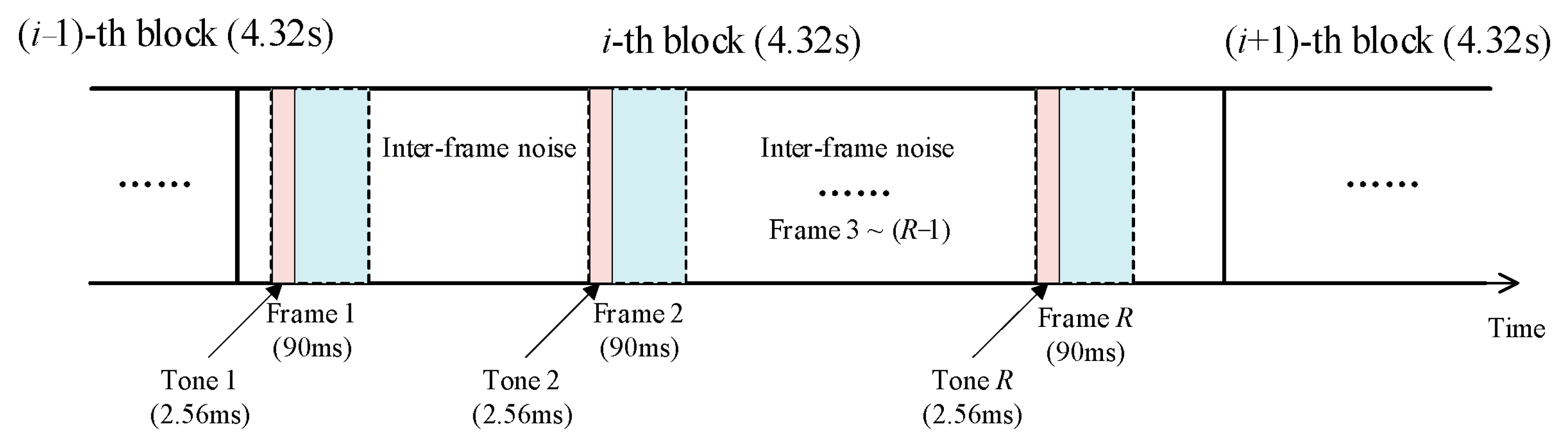
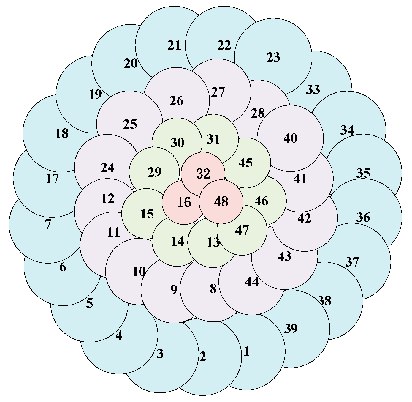
In the second step, as illustrated in Figure 16, the precise localization of tone starting positions for each frame enables accurate partitioning of the block into three distinct components: R tones (pink), intra-frame signals, excluding tones (blue), and inter-frame noise (white). The block can be decomposed into the three components as follows:

$$s_{block}\left[n\right]=\left\{\begin{array}{c}{\displaystyle \sum _{r=1}^R{s}_{tone}\left[n-N_{frame}^r\right]}\\ {\displaystyle \sum _{r=1}^R{s}_{uni}[n-N_{tone}-N_{frame}^r]+{\displaystyle \sum _{r=1}^R{s}_{data}[n-N_{tone}-N_{uni}-N_{frame}^r]}}\\ {\epsilon }_{ex,frame}\left[n\right]\end{array}\right.$$

(14)

where $N_{tone}$ and $N_{uni}$ denote the number of points of one tone and a unique word, respectively. ${\epsilon }_{ex,frame}\left[n\right]$ denotes the inter-frame noise. To perform energy integration for the tone’s SNR calculation, an $N_{tone}$-point FFT is applied to the extracted tone signal, yielding the frequency spectrum of the r-th tone as $S_{tone}^r\left(k\right)$. Through analysis of the spectral peak and noise floor, the SNR of the r-th tone can be estimated as:

$$\widehat{SN{R}^r}={\displaystyle \frac{1}{N_{tone}}}\cdot {\displaystyle \frac{{\left[S_{tone}^r\left(k_0^r\right)\right]}^2}{\left\{{\displaystyle \sum _{k=0}^{N_{tone}-1}{\left[S_{tone}^r\left(k\right)\right]}^2}\right\}-{\left[S_{tone}^r\left(k_0^r\right)\right]}^2}}$$

(15)

where $k_0$ denotes the maximal spectral line of $S_{tone}^r\left(k\right)$.

The frequency offset factor (${\delta }^r$) of each tone can also be estimated from the $N_{tone}$-point FFT, which is performed on the r-th tone:

$${\widehat{\delta }}^r\triangleq {\displaystyle \frac{\left|S_{tone}^r\left(k_0^r+a^r\right)\right|}{\left|S_{tone}^r\left(k_0^r+a^r\right)\right|+\left|S_{tone}^r\left(k_0^r\right)\right|}}$$

(16)

$$a^r=\left\{\begin{array}{cc}1,& \left|S_{tone}^r\left(k_0+1\right)\right|>\left|S_{tone}^r\left(k_0-1\right)\right|\\ -1,& \left|S_{tone}^r\left(k_0+1\right)\right|\le \left|S_{tone}^r\left(k_0-1\right)\right|\end{array}\right.$$

(17)

where $S_{tone}^r$ represents the FFT spectrum corresponding to the r-th tone in the first step, and $k_0^r$ denotes the index of its maximum spectral line of the r-th tone’s spectrum.

Once the SNR and δ of an Iridium NEXT tone signal are determined, this tone is processed by the decision module. The decision module is derived through extensive Monte Carlo simulations conducted over various [SNR, δ] parameter pairs, with the parameter space defined as:

$$SNR\in \left[-15,5\right],\delta \in \left[0,0.5\right]$$

(18)

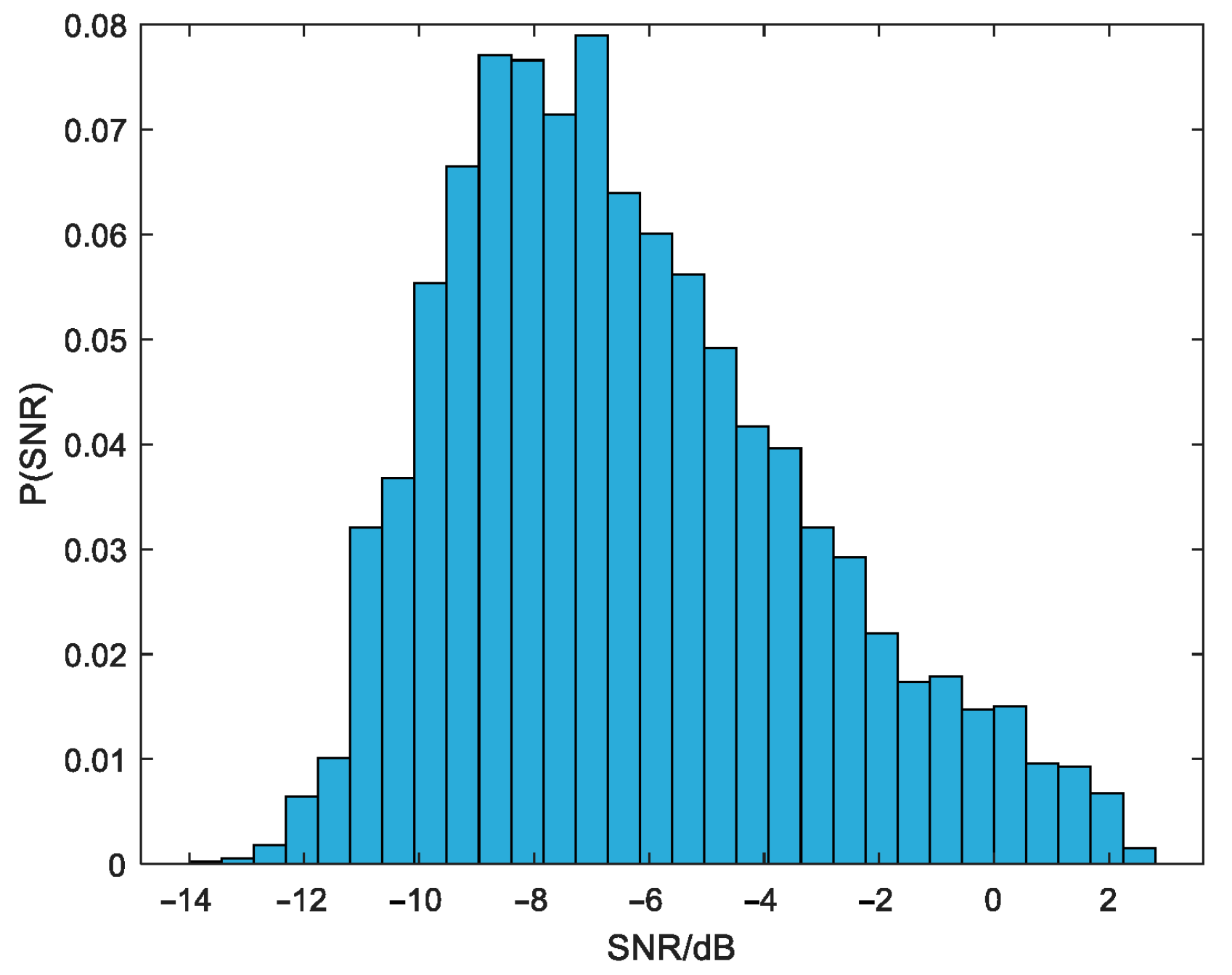
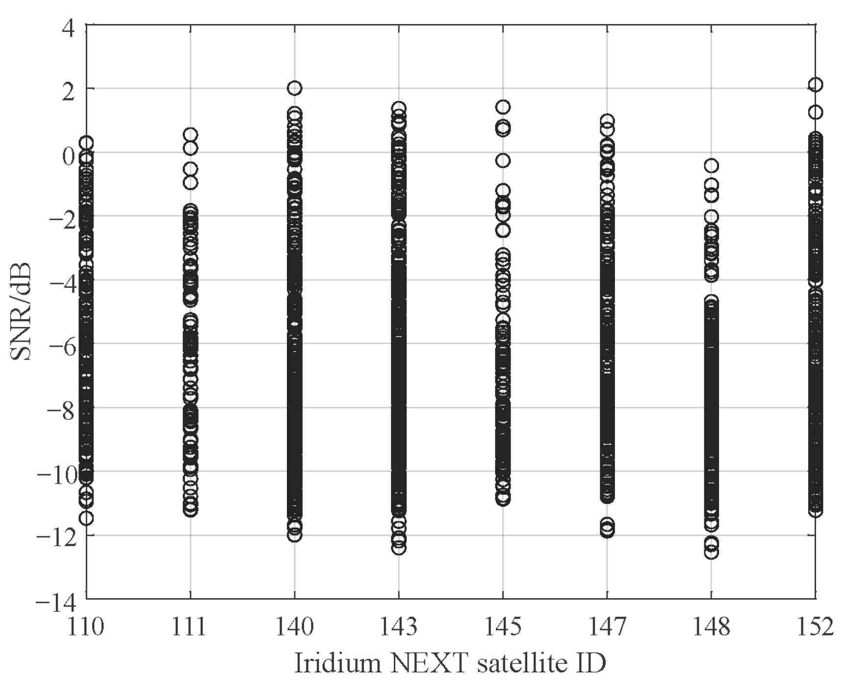
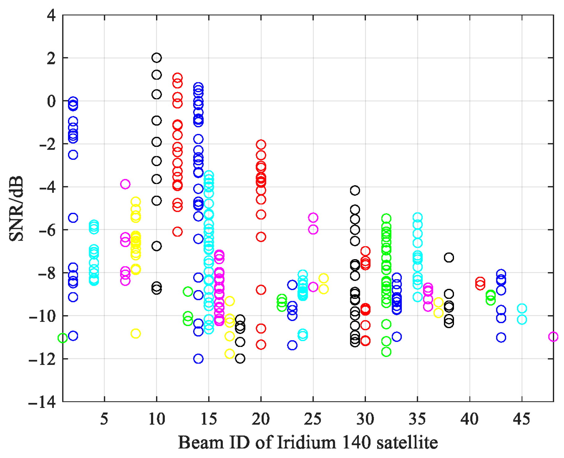
The SNR parameter range is determined based on the measured results from Section 2.3, encompassing the full range of observed SNR values for Iridium signals. The δ parameter range is defined according to Equation (20). For each parameter pair, Monte Carlo simulations were conducted using both the Rife–Vincent algorithm and MLE, with the RMSE calculated for each method. The algorithm yielding the smaller RMSE was selected as the decision label for that parameter pair, which can be expressed as:

$$label\left({\delta }_i,SN{R}_i\right)=\left\{\begin{array}{c}Rife-Vincent,\sqrt{{\displaystyle \sum _{n=1}^{N_{M-C}}\frac{{\left({\widehat{f}}_{n,r-v}-f\right)}^2}{N_{M-C}}}}\le \sqrt{{\displaystyle \sum _{n=1}^{N_{M-C}}\frac{{\left({\widehat{f}}_{n,MLE}-f\right)}^2}{N_{M-C}}}}\\ MLE,\sqrt{{\displaystyle \sum _{n=1}^{N_{M-C}}\frac{{\left({\widehat{f}}_{n,r-v}-f\right)}^2}{N_{M-C}}}}>\sqrt{{\displaystyle \sum _{n=1}^{N_{M-C}}\frac{{\left({\widehat{f}}_{n,MLE}-f\right)}^2}{N_{M-C}}}}\end{array}\right.$$

(19)

where $N_{M-C}$ denotes the number of Monte Carlo simulations performed for each parameter pair, ${\widehat{f}}_{n,r-v}$ and ${\widehat{f}}_{n,MLE}$ denote the estimation result obtained using the Rife–Vincent algorithm and MLE, respectively, and $f$ denotes the true frequency. Based on the obtained decision labels for a large number of [SNR, δ] parameter pairs across the parameter space at fixed step intervals, a K-Nearest Neighbors (KNN) algorithm was employed to decide the r-th tone’s refined Doppler estimation algorithm. Firstly, compute the Euclidean distance between the point corresponding to the parameters of the r-th tone on the plane and all points obtained through simulation as follows:

$$d_i^r=\sqrt{{\left(SN{R}^r-SN{R}_i\right)}^2-{\left({\delta }^r-{\delta }_i\right)}^2}$$

(20)

Then, all $d_i^r$ are sorted in ascending order to form an ordered distance sequence, from which the top K points with the smallest distances are selected to constitute the decision set $J^r$, which can be expressed as:

$$d_{\left(1\right)}^r\le d_{\left(2\right)}^r\le \dots \le d_{\left(K\right)}^r\le d_{\left(K+1\right)}^r\le \dots$$

(21)

$$J^r=\left\{d_{\left(1\right)}^r,d_{\left(2\right)}^r,\dots ,d_{\left(K\right)}^r\right\}$$

(22)

Subsequently, the decision weights for the Rife–Vincent algorithm and the MLE can be computed, respectively, as:

$$\begin{array}{l}{W}_{Rife-Vincent}^r={\displaystyle \sum _{j=1}^K\frac{\mathbb{I}\left(labe{l}_{\left(j\right)}=Rife-Vincent\right)}{d_{\left(j\right)}+\Delta }},d_{\left(j\right)}\in J^r\\ W_{MLE}^r={\displaystyle \sum _{j=1}^K\frac{\mathbb{I}\left(labe{l}_{\left(j\right)}=MLE\right)}{d_{\left(j\right)}+\Delta }},d_{\left(j\right)}\in J^r\end{array}$$

(23)

where $labl{e}_{\left(j\right)}$ denotes the tag corresponding to $d_{\left(j\right)}^r$, $\mathbb{I}\left(\cdot \right)$ is the indicator function (which equals 1 if the condition is satisfied and 0 otherwise), and $\Delta$ is a small constant introduced to prevent division by zero. Finally, the decision result of the r-th tone can be derived by comparing the two weight parameters:

$$decisio{n}^r=\left\{\begin{array}{c}Rife-Vincent,W_{Rife-Vincent}^r\ge W_{MLE}^r\\ MLE,W_{Rife-Vincent}^r<W_{MLE}^r\end{array}\right.$$

(24)

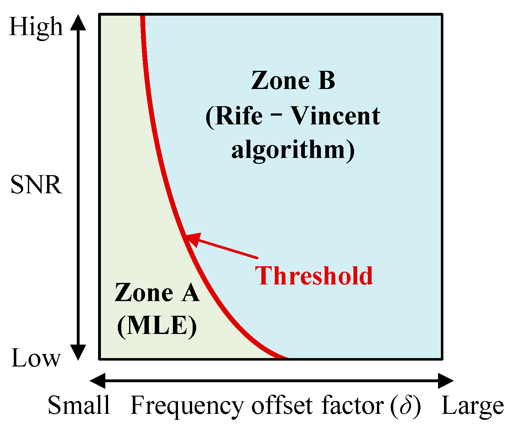
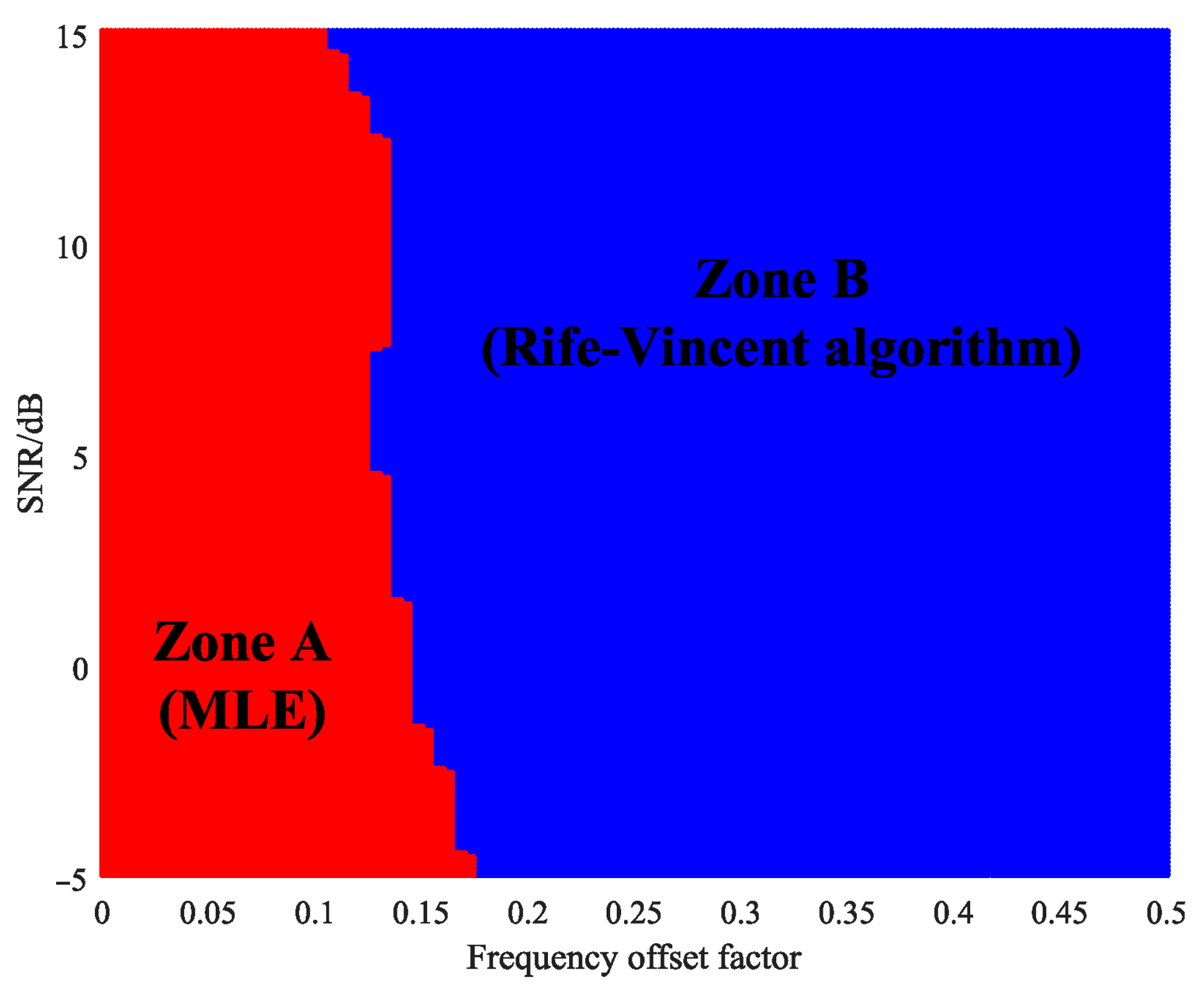
The decision module can be divided into two distinct zones (Figure 17): Zone A—low δ values and mainly low SNR—and Zone B—higher δ values and mainly high SNR. The decision module then classifies each Iridium NEXT tone signal on the basis of its SNR and δ values: tone signals classified into Zone A are processed with the MLE method, whereas those classified into Zone B are processed with the Rife–Vincent algorithm. By adaptively selecting the most suitable algorithm for each tone signal, the decision module improves the Doppler frequency estimation accuracy relative to existing single-algorithm methods.

In the third step, the preliminary FFT results (${\widehat{f}}_1^r$) are compensated by applying the selected processing algorithm to estimate the required Doppler frequency compensation (${\widehat{f}}_2^r$). Algorithm selection can strongly influence the operational complexity of the estimation process. If the Rife–Vincent compensation algorithm [21] is selected, the residual correction estimate ${\widehat{f}}_2^r$ is calculated as:

$${\widehat{f}}_2^r={\displaystyle \frac{f_s}{N_{FFT}}}\cdot a^r\cdot {\delta }^r$$

(25)

where a is the compensation direction defined as in Equation (18), ${\delta }^r$ is the frequency offset factor defined as in Equation (17), $f_s$ is the sampling frequency, and $N_{FFT}$ is the number of FFT sampling points.

However, if the MLE method is selected instead, the Iridium NEXT tone signal is first down-converted to a low-frequency signal $s_{tone,LF}^r\left[n\right]$ using the FFT-estimated Doppler frequency ${\widehat{f}}_1^r$:

$$s_{tone,LF}^r\left[n\right]=s_{tone}^r\left[n\right]\cdot \exp \left(-j2\pi {\widehat{f}}_1^{r}n/f_s\right)$$

(26)

The residual correction value is then derived by MLE comparison. The comparison function can be expressed as:

$$I^r\left(f\right)={\left|{\displaystyle \sum _{n=0}^{N-1}{s}_{tone,LF}^r\left[n\right]\cdot \exp \left(-j2\pi fn/f_s\right)}\right|}^2$$

(27)

then, the accurate residual correction estimate of the r-th tone in the block ${\widehat{f}}_2^r$ is the value that minimizes the comparison function, i.e.,

$${\widehat{f}}_2^r=\underset{f}{\arg \min }\left[I\left(f\right)\right]$$

(28)

The final, accurate Doppler frequency estimate combines the preliminary FFT estimate (${\widehat{f}}_1^r$) with the residual correction (${\widehat{f}}_2^r$):

$${\widehat{f}}_d^r={\widehat{f}}_1^r+{\widehat{f}}_2^r$$

(29)

4. Simulation Results

4.1. Dual-Constraint KNN-Based Decision Model

For this simulation, we generated synthetic Iridium NEXT tone signals with MATLAB (version 2021b) using the signal parameters listed in

Table 2. Input parameters for synthetic Iridium NEXT tone signal simulations.

Parameter Name	Value
SNR	−15 dB to 5 dB
Frequency offset factor	0–0.5
Doppler frequency	0–40 kHz
Signal duration	2.56 ms
Sampling rate	2.5 MHz

. To evaluate the domain of optimal performance of both Doppler frequency estimation algorithms, we conducted Monte Carlo simulations for the Rife–Vincent and MLE algorithms under controlled parameter variations: SNR variations (range given in Table 1) in 1-dB increments and δ variations in 0.01 increments across the Iridium NEXT operational range. For each (δ, SNR) parameter pair, we ran 1000 independent Monte Carlo simulations to provide statistical significance, using the RMSE as a primary metric to assess the estimation accuracy.

The decision label of each parameter pair (Figure 18B) was then determined by comparing the simulated RMSE of each parameter (Figure 18A). Based on the simulated parameter pairs and labels, a KNN classification model was trained in the parameter space to classify each input parameter pair.

In the KNN algorithm, K is a critical parameter representing the number of neighboring points involved in the decision-making process. To determine the optimal value of the critical parameter K in the KNN algorithm, we conducted 10,000 Monte Carlo experiments to evaluate the performance of the KDFE algorithm under different K values. The experimental results presented in

Table 3. RMSE (Hz) of the KDFE algorithm under different K values.

K = 1	K = 2	K = 3	K = 4	K = 5	K = 6	K = 7	K = 8
15.34	15.18	14.85	14.85	14.69	15.07	15.26	15.50

demonstrate that when K is too small, the model becomes overly complex and suffers from overfitting, while when K is too large, the model becomes oversimplified and exhibits underfitting. The KDFE algorithm achieves its optimal performance at K = 5, which is consequently selected as the K-value for the KNN algorithm in this study.

To evaluate the classification performance of the KNN algorithm for each tone’s parameter pair, we simulated input parameter pairs across the parameter space with an SNR step size of 0.1 and a frequency offset factor step size of 0.002. The classification results of the KNN classification model for each simulated parameter pair are presented in Figure 19. In Zone A, where δ values are small, the decision module selected the MLE method, which is more robust; in Zone B, corresponding to larger δ values, the Rife–Vincent algorithm was selected instead, owing to its higher accuracy and computational efficiency. For intermediate δ values, which are neither too large nor too small (0.13 < δ < 0.18), the SNR becomes an important parameter for the decision module. In this case, the Rife–Vincent algorithm was selected because of its robustness when the SNR was moderately small, whereas the MLE method was selected because of its high accuracy when the SNR was moderately large. The simulated threshold was very consistent with the theoretical analysis, confirming the pertinence of our approach and the usefulness of the dual-constraint decision module.

4.2. Evaluation of the Doppler Frequency Estimation Accuracy

Here, we conducted additional Monte Carlo experiments covering the same SNR conditions (from −15 dB to 5 dB in increments of 1 dB) but with random δ variations to evaluate the accuracy of our proposed KDFE algorithm. The input simulation parameters were unchanged (Table 2). For each SNR value, we conducted 50,000 Monte Carlo experiments with random δ values. The adaptability of the dual-constraint decision module, core innovation of the proposed algorithm, was first evaluated by verifying the proportion of use of both estimation algorithms for the simulated Iridium NEXT tone signals. As illustrated in Figure 20, the decision module dynamically adjusted algorithm selection to the characteristics of each tone signal, resulting in a utilization ratio in very good agreement with the previous simulations; the decision module preferentially selected the Rife–Vincent algorithm to process the simulated tone signals with smaller δ values and switched to MLE for larger δ values. In transitional cases with δ close to the threshold value, SNR became the dominant constraint. Under these intermediate conditions, the decision module adopted a hybrid, adaptive approach, selecting either algorithm on the basis of real-time SNR evaluation for individual tone signals.

From these simulations, we also compared the RMSE results for the proposed KDFE algorithm, as a function of the SNR, with those obtained with the standard FFT, Rife–Vincent, and MLE algorithms (Figure 21). Under SNR conditions corresponding to the typical range of Iridium NEXT signals, the KDFE algorithm achieved a substantially higher estimation accuracy than the standard FFT algorithm and an accuracy improvement at the Hz level, compared with the Rife–Vincent algorithm, under all SNR conditions. Compared with the MLE method, the KDFE accuracy was similar for moderately large SNR values (>0 dB) but considerably higher for smaller SNR values (<0 dB). Therefore, because Iridium NEXT tone signals with SNR > 0 dB represent only 4.5% of the total (Figure 6), our results imply that the estimation accuracy of the proposed algorithm was higher than that of the MLE method. These results clearly demonstrate the high accuracy of the KDFE algorithm for Doppler frequency estimation in more realistic scenarios.

4.3. Accuracy Evaluation Using a Simulated Iridium NEXT Signal

We simulated a complete observation arc for one Iridium NEXT signal, consisting of 138 discontinuous frames over a period of 10 min. The simulation parameters are listed in

Table 4. Simulation parameters for a complete Iridium NEXT observation arc.

Parameter Name	Value
Orbit altitude	785 km
Satellite orbital velocity	7464 m/s
Simulation duration	600 s
Pilot duration	2.56 ms
Sampling rate	2.5 MHz
Carrier frequency	1626.229168 MHz
SNR	−15 dB to 5 dB
Effective isotropic radiated power	−90 dBmW

. We applied all algorithms—FFT, Rife–Vincent, MLE, and KDFE—to estimate the Doppler frequencies of the 138 tone signals and calculate the corresponding RMSE.

Over the simulation duration, the simulated Doppler frequency varied within ±40 kHz, with notable changes between consecutive frames (Figure 22).

During the 10 min simulation period, the proposed KDFE algorithm was more accurate than the three reference algorithms, FFT, MLE, and Rife–Vincent (Figure 23). The calculated RMSE values were 111.7 Hz, 31.25 Hz, 19.8 Hz, and 14.6 Hz for the FFT, MLE, Rife–Vincent, and KDFE algorithms, respectively. Compared with the Rife–Vincent and MLE results, the KDFE algorithm yielded accuracy improvements of 26.3% and 82.9%, respectively, clearly demonstrating the higher performance of our proposed algorithm.

5. Experimental Application to Real Iridium NEXT Signals

5.1. Experiment Setup

To evaluate the effective KDFE performance for SoOP positioning, we also conducted field experiments using a self-constructed reception and processing platform for Iridium NEXT signals (Figure 24). The platform comprises an Iridium NEXT antenna (JCYX008; Zhejiang JC Antenna Co., Ltd., Jiaxing, Zhejiang Province, China), a universal software radio peripheral (USRP B210, Ettus Research, Austin, TX, USA), a laptop computer (Lenovo ThinkPad X1, Lenovo, Beijing, China), and a portable power supply. Iridium NEXT signals received by the antenna are sampled at a 2.5 MHz rate, down-converted by the USRP, and stored by a Python-based software-defined radio (SDR) receiver. The baseband signals are then transferred to the computer for epoch acquisition, decoded to obtain the satellite ID, and timestamped. Positioning calculations are processed with dedicated MATLAB code. In addition, some key parameters in the experiment are shown in

Table 5. Experimental parameter settings for Iridium NEXT signal receiving.

Parameter Name	Value
Sampling rate	2.5 MHz
Center frequency	1626.229168 MHz
Bandwidth	2.6 MHz
Frame duration	90 ms
Tone duration	2.56 ms
SNR threshold	>−20 dB

.

5.2. Doppler Frequency Estimation Accuracy Test

To evaluate the Doppler frequency estimation accuracy of the proposed algorithm, we conducted a long-term field experiment. This experiment was conducted at the Advanced Technology Research Base of the Chinese Academy of Sciences in Beijing, China. We collected Iridium NEXT signal data for 60 min. Because the Iridium NEXT duplex channels only broadcast signals to requesting users, we exclusively acquired signals from the simplex channel. During the monitoring period, we acquired data for 2472 epochs from 16 distinct Iridium NEXT satellites (Figure 25); tracked 11 complete and 3 partial satellite transit arcs; and collected a few epochs only for 2 satellites.

As in the simulations (Section 4.3), we applied four methods to process the acquired Iridium NEXT tone signals and estimate their Doppler frequency: FFT, MLE, Rife–Vincent, and KDFE. The estimations clearly exhibited characteristics consistent with typical Doppler frequency curves of LEO satellites (Figure 26). For comparison, we derived Doppler frequencies using a combination of two-line orbital element (TLE) ephemerides retrieved from the CelesTrak website [35] and output data from the Simplified General Perturbations version 4 (SGP4) model; all our experimental tests occurred within 8 h of TLE updates. The orbit and velocity errors presented in Figure 27 were obtained by comparing the predicted results from the TLE combined with the SGP4 model to a reference orbit. The reference orbit was generated using the High Precision Orbit Propagator model configured in the Systems Tool Kit simulation software (Systems Tool Kit 11.8). During the time window between TLE update and observation (<8 h), the SGP4 satellite orbit prediction remained highly accurate. Consequently, we conclude that Doppler frequency predictions from the SGP4 model constitute excellent references. In this work, since the indicators of each algorithm are the statistical averages of a large number of trials, the frequency error of the satellite is not considered.

As shown in Figure 26, the KDFE algorithm not only demonstrates significantly better estimation accuracy than FFT but also exhibits closer alignment with the Doppler frequency predicted by the SPG4 model when compared to both MLE and Rife–Vincent algorithms, indicating superior estimation precision. Using the SGP4 predictions as a reference, we calculated the Doppler frequency estimation error for all acquired epoch data and derived the corresponding RMSE. The proposed KDFE algorithm achieved consistently higher accuracy than the Rife–Vincent and MLE algorithms. Statistical analysis of the 2472 epochs yielded RMSE values of 124.85 Hz, 37.51 Hz, 16.32 Hz, and 12.03 Hz with the FFT, MLE, Rife–Vincent, and KDFE algorithms, respectively. By comparing this result with the simulation results of the three algorithms in Section 4.3, it can be known that the maximum RMSE gap between the two does not exceed 18%, which fully cross-verifies the reliability of the simulation and experiment. Compared to conventional FFT, Rife–Vincent, and MLE methods, the proposed algorithm improves Doppler frequency estimation accuracy by 90.36%, 67.93%, and 26.29%, respectively. These results further demonstrate that the proposed algorithm achieved markedly higher Doppler frequency estimation accuracy than existing standard methods.

5.3. Positioning Accuracy Test

To validate the positioning performance of the proposed algorithm, we conducted a series of SoOP positioning experiments. Over a 24 h observation period, 11 independent experimental trials were performed, each with a 20 min continuous data collection window. During these trials, a total of 7337 Iridium frames were captured. The captured Iridium frames were processed using three distinct Doppler frequency estimation approaches: proposed KDFE, the conventional Rife–Vincent algorithm, and MLE. To exclude the impact of different positioning algorithms from positioning estimation, all trials employed batch least-squares estimation for position estimation.

Table 6. Comparison of SoOP positioning results from the Rife–Vincent, MLE, and KDFE algorithms.

Trial Number	Total Epochs	3D Positioning Error/m
		KDFE	Rife–Vincent	MLE
1	703	218.07	250.03	285.77
2	487	495.36	576.87	384.77
3	553	240.20	327.51	1010.44
4	477	266.66	267.99	348.45
5	648	76.18	93.63	740.82
6	662	347.87	366.08	332.04
7	654	250.39	329.48	1125.32
8	737	450.15	467.65	87.11
9	1004	329.57	338.07	683.04
10	701	172.63	186.00	221.85
11	711	154.92	337.19	210.91
RMSE		297.92	344.70	592.79

presents the 3D positioning errors obtained from 11 independent trials using Doppler frequency estimates derived from the proposed KDFE algorithm, Rife–Vincent algorithm, and MLE. The proposed algorithm consistently outperformed the Rife–Vincent approach across all trials, achieving Doppler frequency estimation accuracy improvements ranging from 54% to 1%. Compared to MLE, the proposed method demonstrated significantly superior accuracy in most trials. Although MLE exhibited better positioning precision in a few isolated trials, the proposed algorithm achieved substantially lower RMSE due to its exceptional robustness. These experimental results are consistent with the characteristics of various algorithms demonstrated in the simulation. Across all 11 trials, the RMSE values were 297.92 m (proposed), 344.70 m (Rife–Vincent), and 592.79 m (MLE), representing positioning accuracy improvements of 13.57% and 49.74% over Rife–Vincent and MLE, respectively.

Figure 28 presents the field distribution of SoOP positioning results and corresponding RMSE ranges obtained using the three algorithms. While the Rife–Vincent algorithm produces a spatial distribution similar to our proposed method, the proposed algorithm obtained better positioning estimation accuracy than Rife–Vincent in each trial. Hence, the proposed algorithm achieves higher estimation accuracy. Although the MLE algorithm achieves satisfactory results in a few isolated trials, its poor stability and insufficient robustness lead to a significantly wider distribution of positioning results and consequently larger RMSE values. Our field experiment thus demonstrated that higher accuracy in the Doppler frequency estimation, such as that provided by the proposed algorithm, is essential to improve SoOP positioning.

6. Conclusions

In this study, we first summarize three models of Iridium SNR fluctuations based on long-term observations and the characteristics of Iridium beams. On this basis, we established the KDFE algorithm, an original approach to high-accuracy Doppler frequency estimation from Iridium tone signals. By combining the Rife–Vincent algorithm and MLE method with a KNN-based decision module, the KDFE algorithm adaptively selects the optimal estimation strategy accounting for a dual constraint on the SNR and frequency offset factor δ. The algorithm first calculates a coarse FFT estimate, and then the KNN-based decision module dynamically selects one of the algorithms to compensate for the result, depending on the signal position in the SNR–δ plane. Extensive Monte Carlo simulations confirmed that our KDFE algorithm clearly outperforms the Rife–Vincent and MLE algorithms under typical Iridium NEXT operational conditions. Indeed, experimental results with simulated signals evaluated the Doppler estimation error reduction provided by the KDFE algorithm at 26.3% and 82.9% relative to the Rife–Vincent and MLE algorithms, respectively. Finally, we conducted a series of field trials for SoOP positioning from acquired Iridium NEXT signals. The RMSE of KDFE positioning was 297.92 m, representing improvements of 13.57% and 49.74% on the Rife–Vincent and MLE values, respectively. Our results clearly emphasize the high performance of the proposed algorithm that improves both Doppler frequency estimation and downstream SoOP positioning performance. In the future, we will explore more possibilities of using artificial intelligence algorithms to intelligently preprocess LEO signals.