
A Novel Joint Denoising Strategy for Coherent Doppler Wind Lidar Signals

 and
and
Abstract
1. Introduction
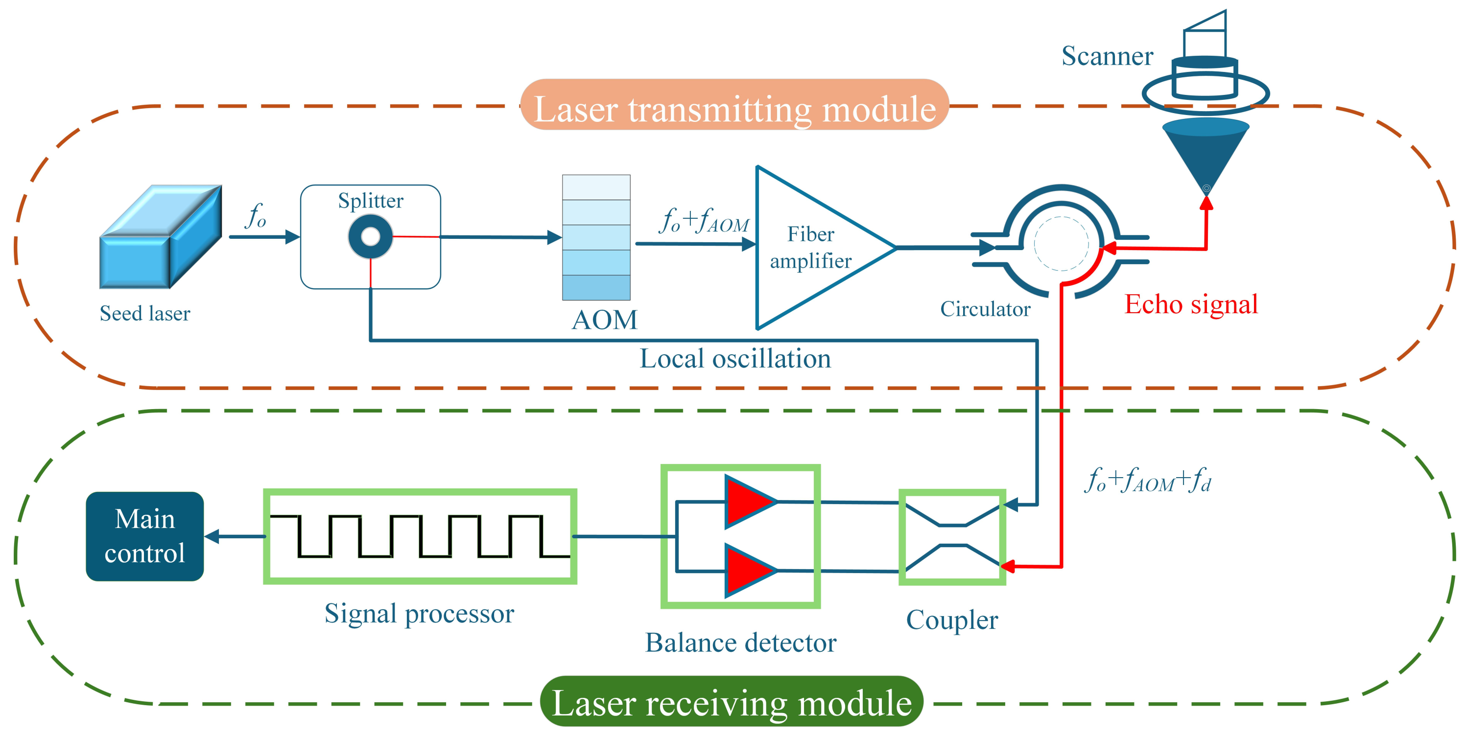
2. Principle of Coherent Doppler Wind Lidar
3. SVD-ICEEMDAN-SCC-MF Methodology
3.1. SVD
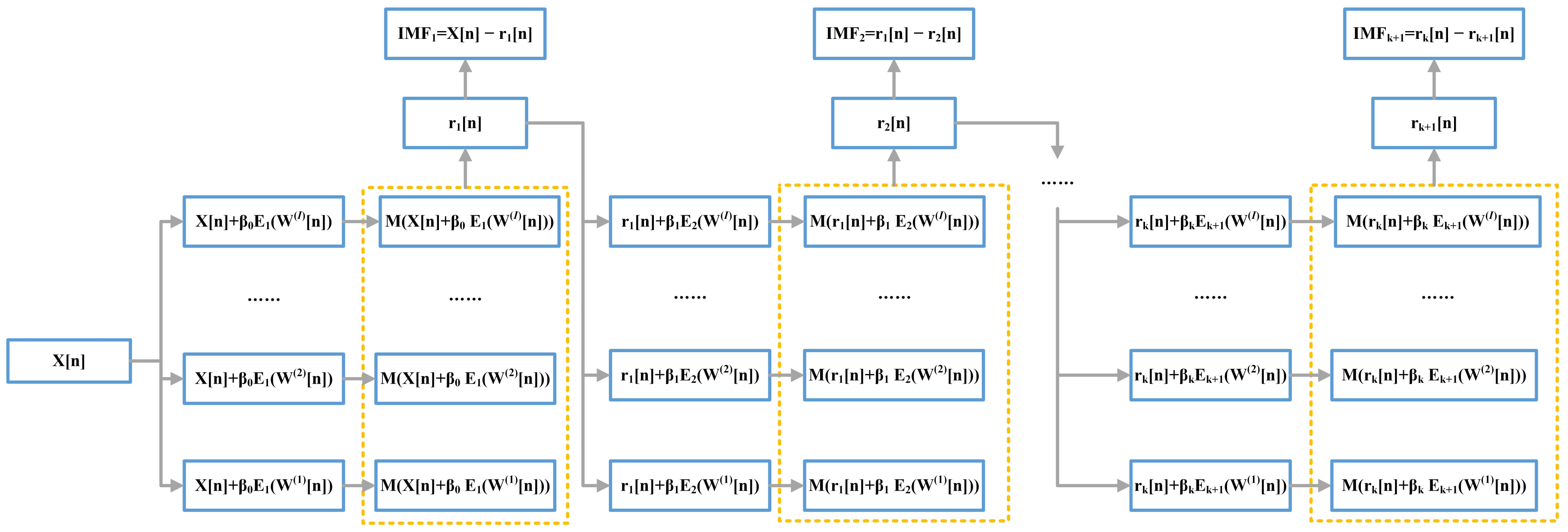
3.2. ICEEMDAN
3.3. Spearman Correlation Coefficient
3.4. Median Filtering
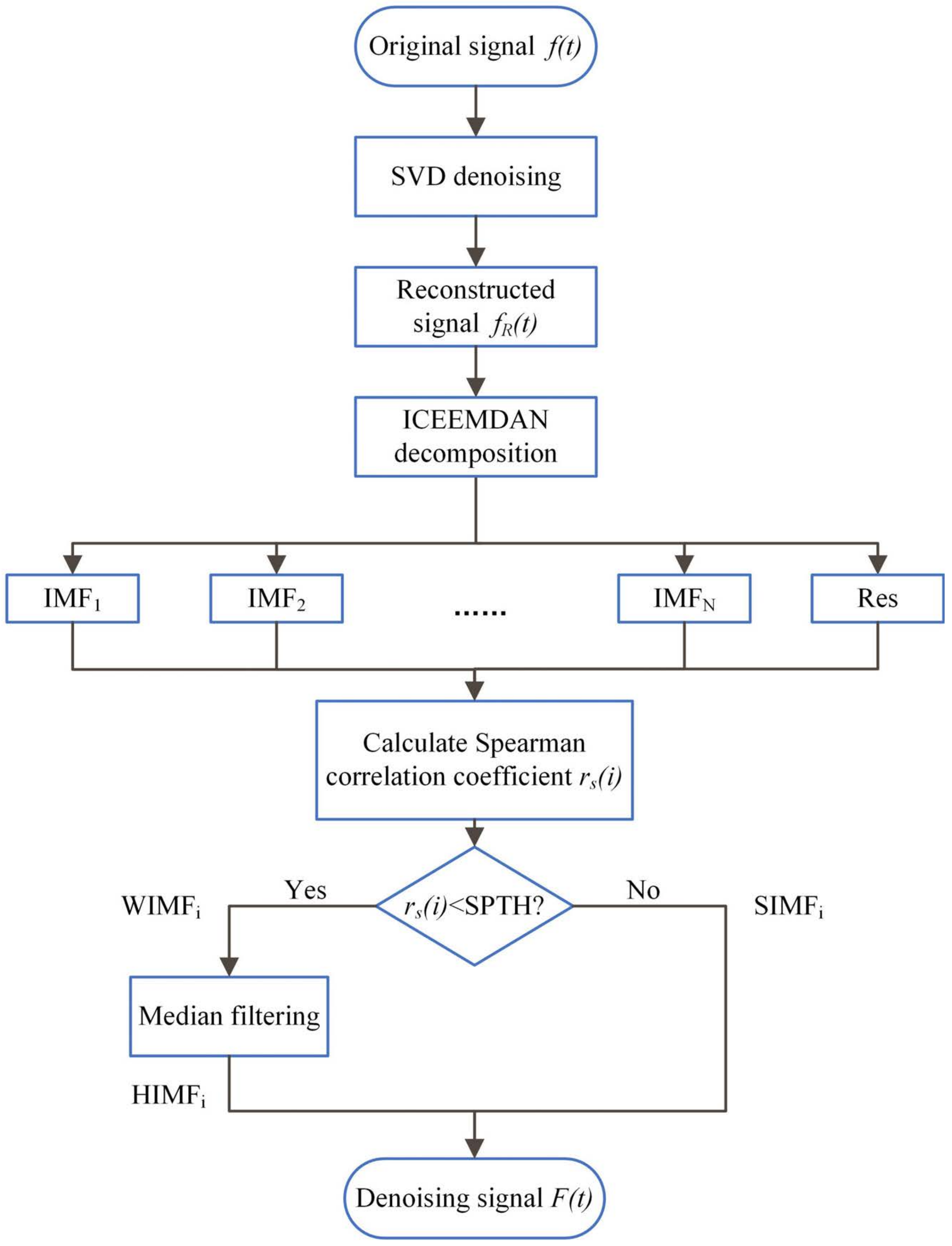
3.5. SVD-ICEEMDAN-SCC-MF Algorithm
- If yes, the component is weakly correlated with the reconstructed signal , then the component is ready for median filtering, which is noted as .
- If no, then the component is strongly correlated with the reconstructed signal , then the component is not processed, and the component is recorded as .
4. Results
4.1. Evaluation Indicators
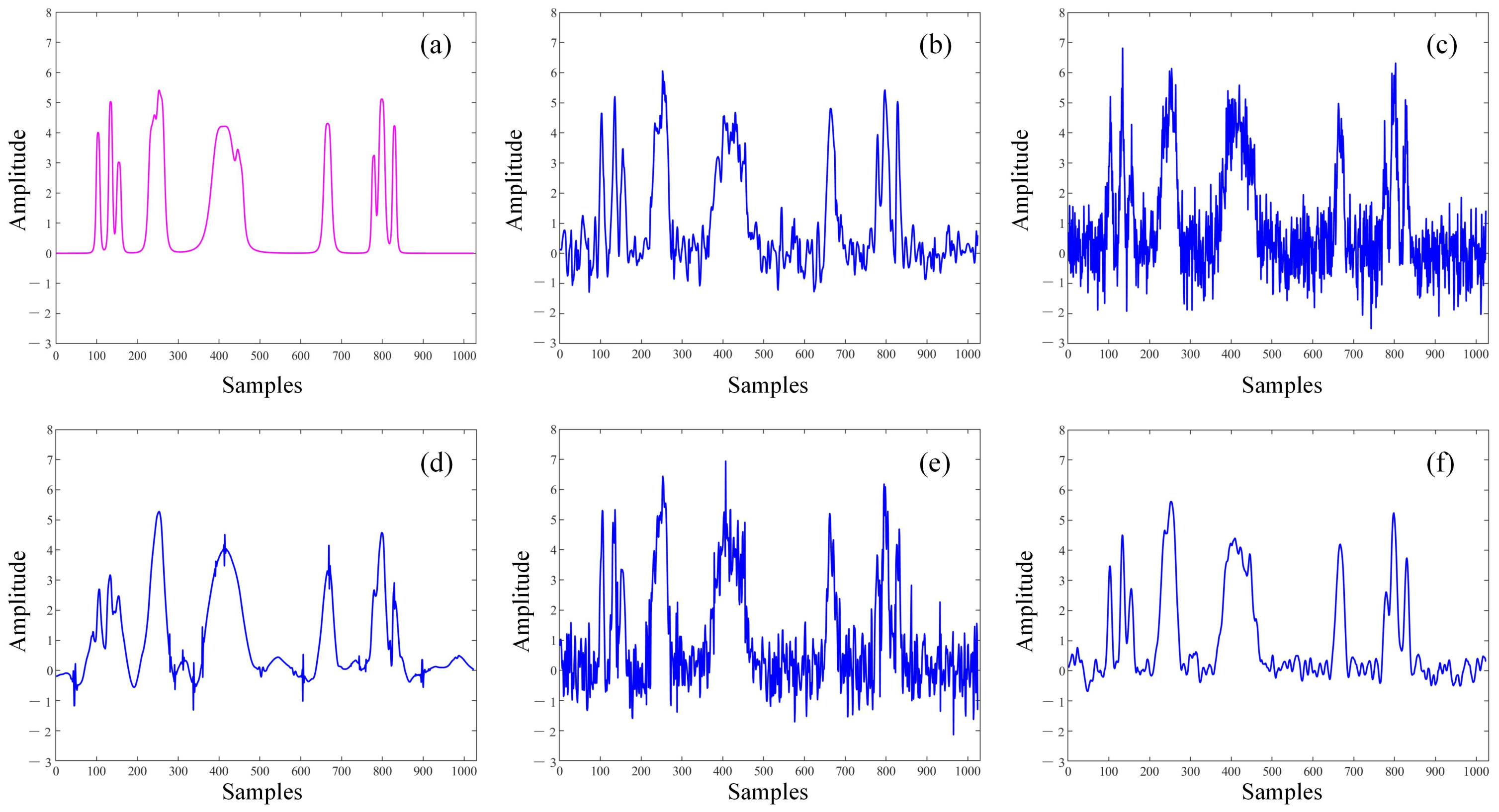
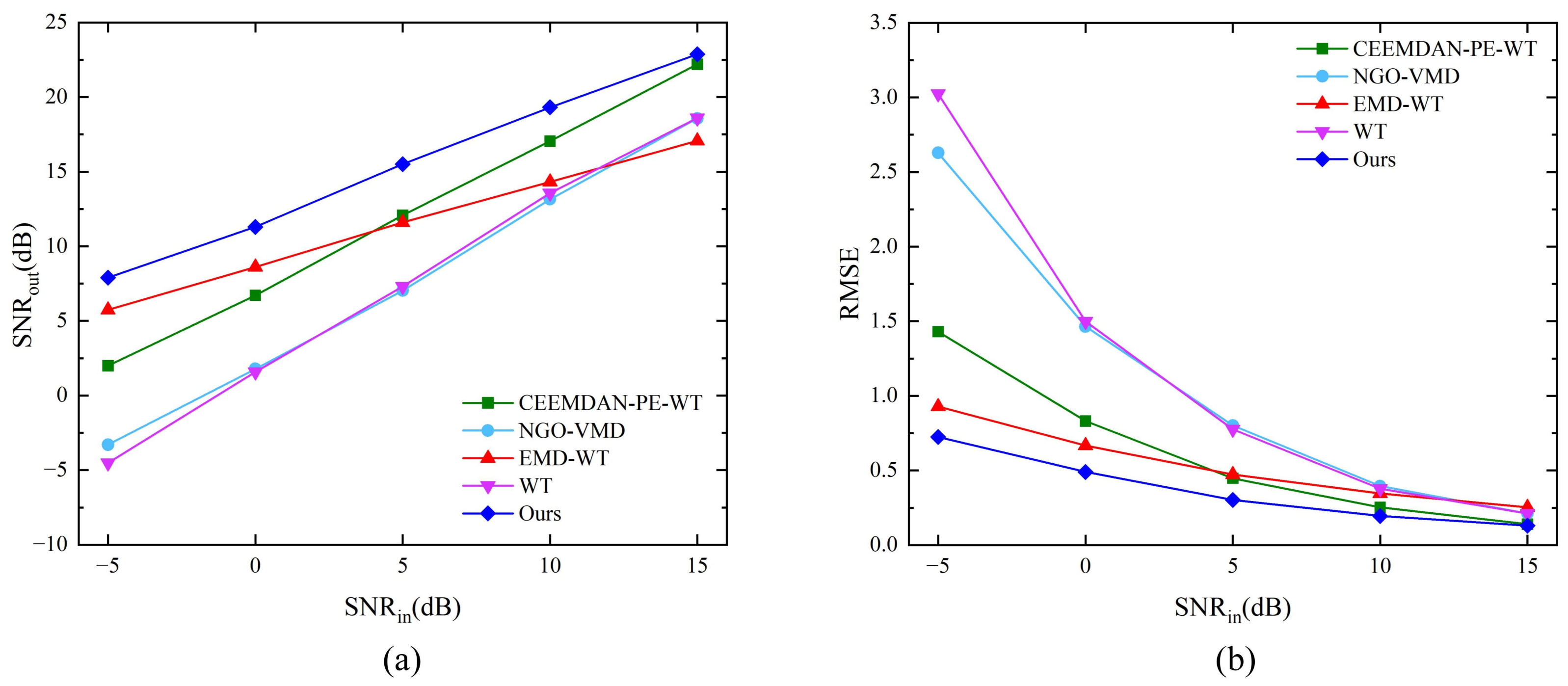
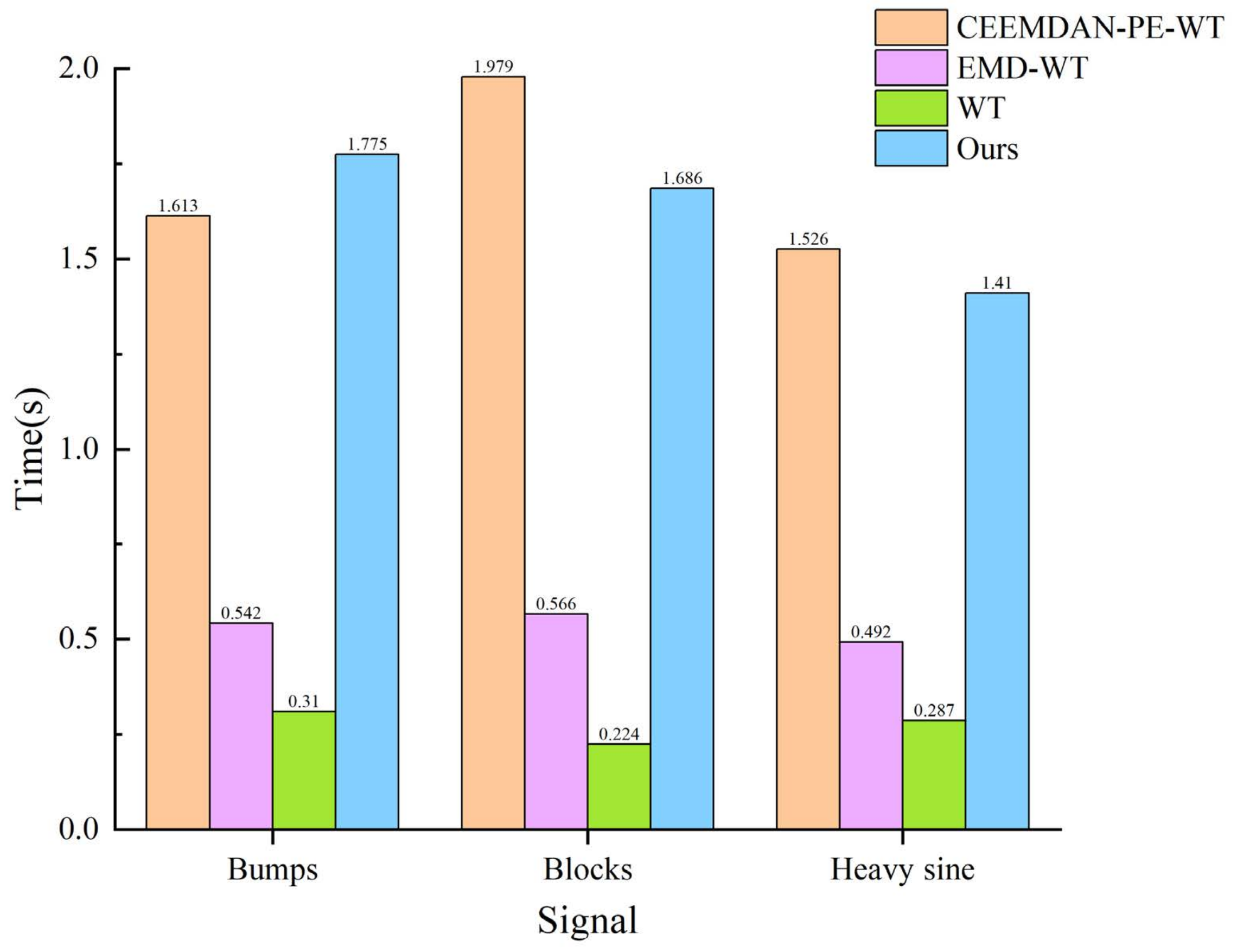
4.2. Analogue Signal Denoising Experiment
4.3. CDWL Simulation Signal Denoising Experiment
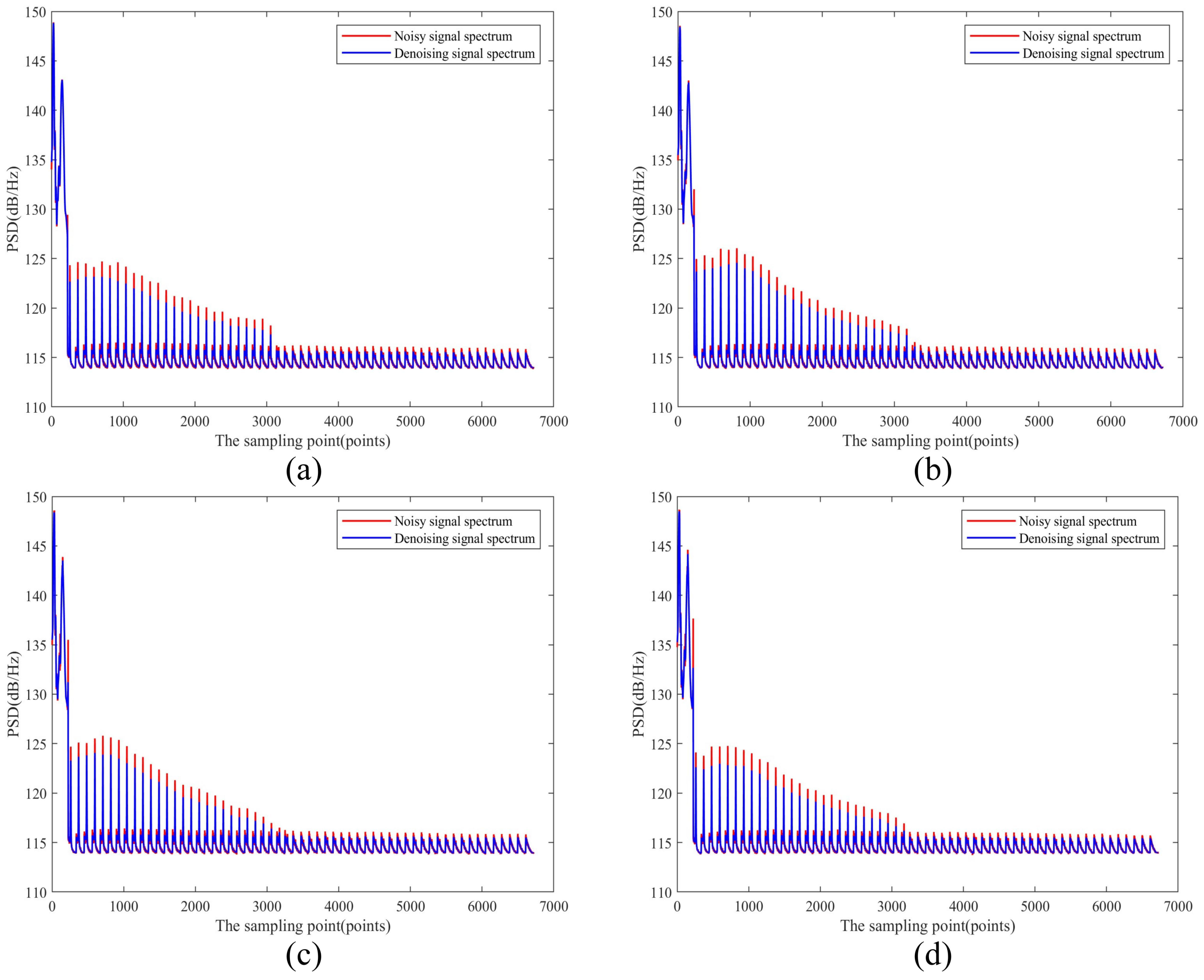
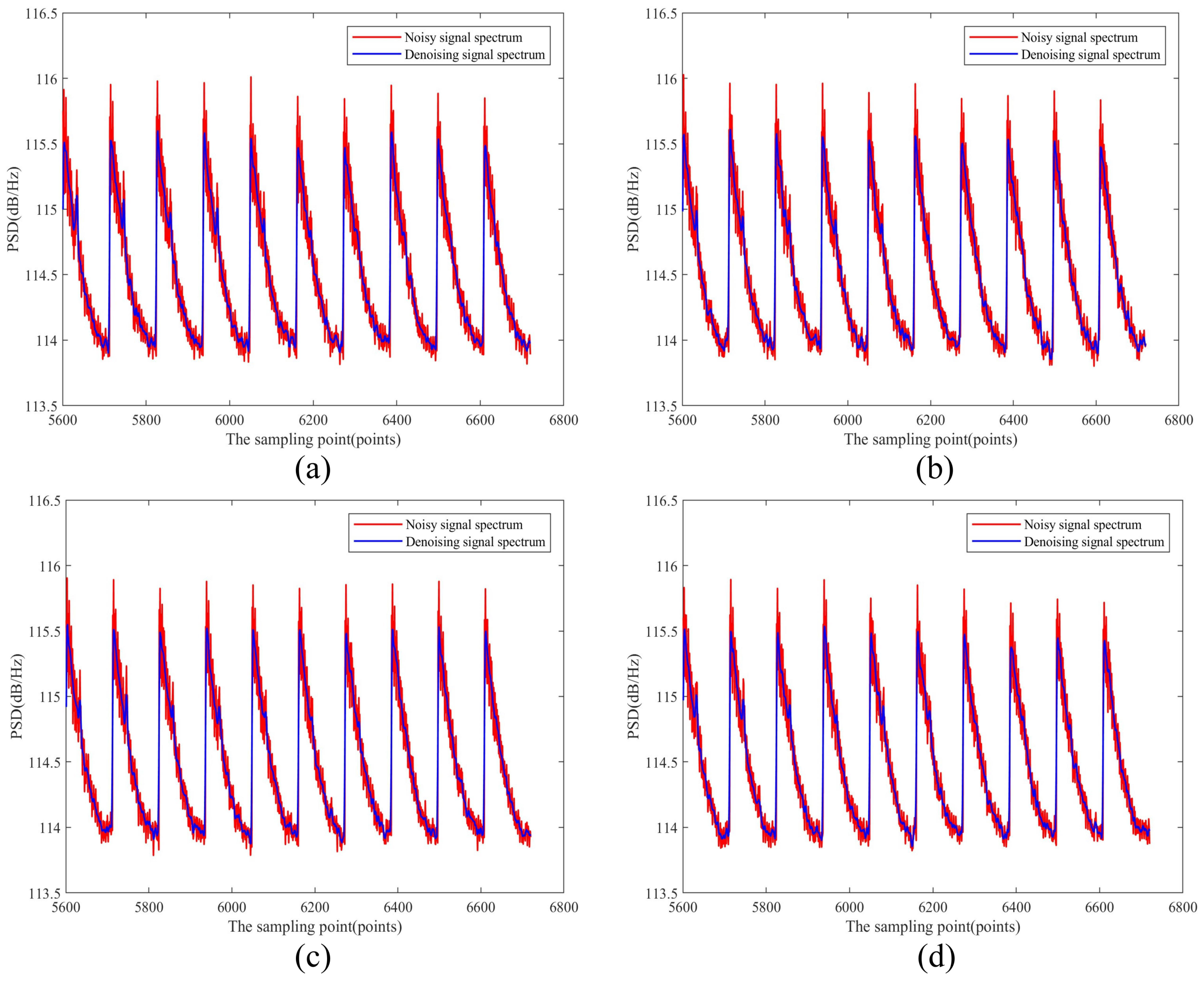
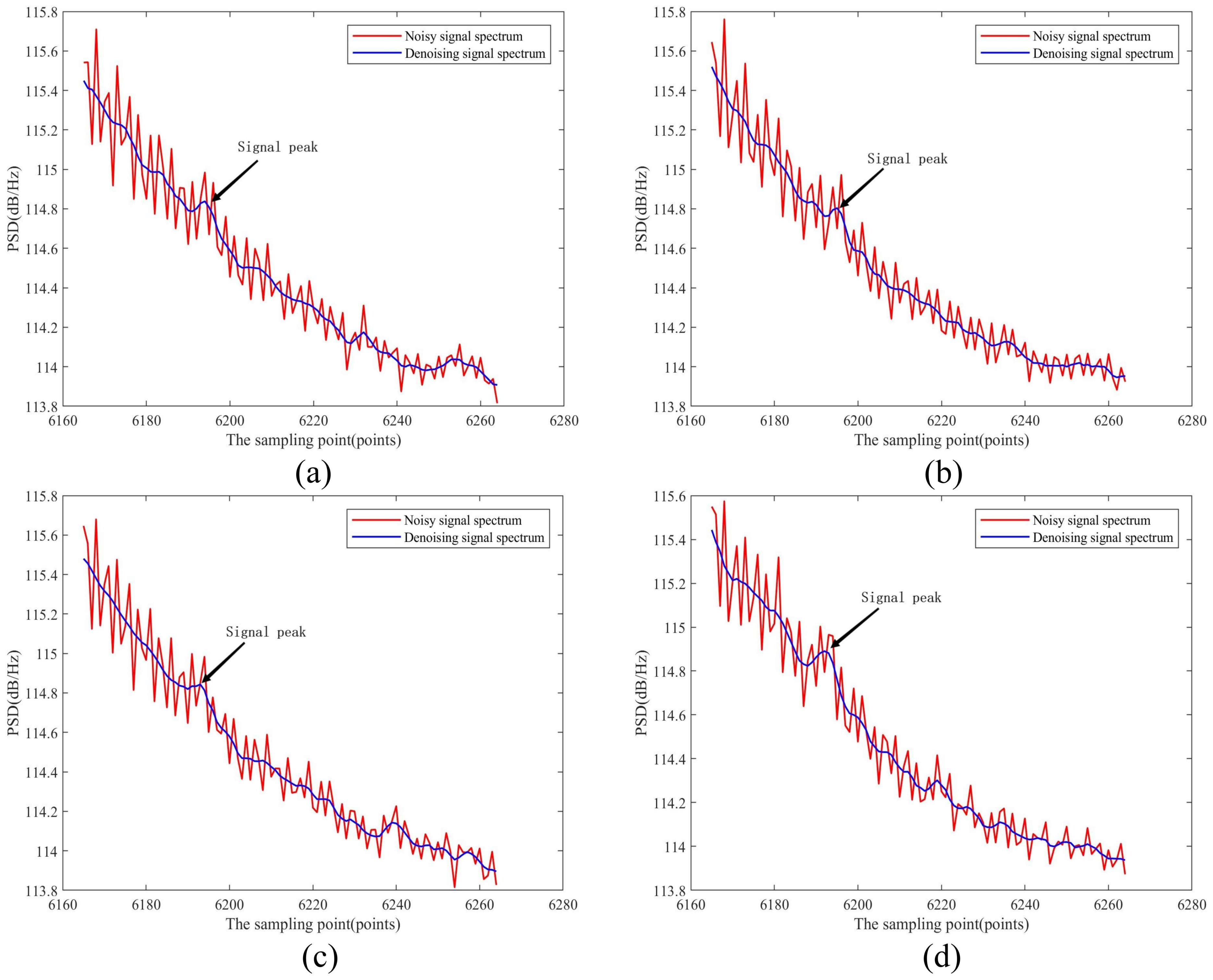
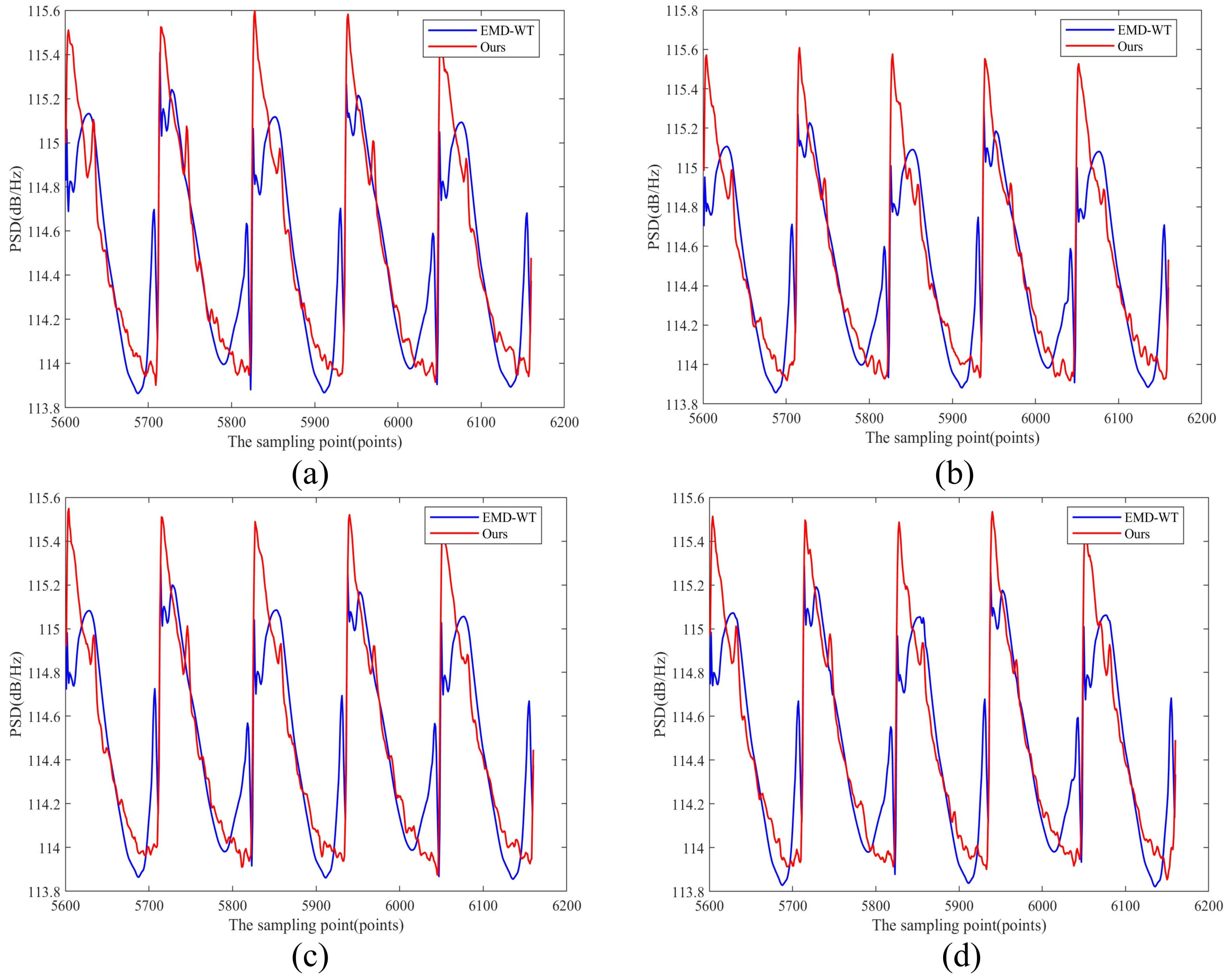
4.4. Real CDWL Signal Denoising Experiment
5. Conclusions
Author Contributions
Funding
Data Availability Statement
Conflicts of Interest
References
- Kane, T.J.; Kozlovsky, W.J.; Byer, R.L.; Byvik, C.E. Coherent laser radar at 1.06 μm using Nd:YAG lasers. Opt. Lett. 1987, 12, 239–241. [Google Scholar] [CrossRef] [PubMed]
- Proctor, F.; Hamilton, D. Evaluation of Fast-Time Wake Vortex Prediction Models. In Proceedings of the 47th AIAA Aerospace Sciences Meeting including The New Horizons Forum and Aerospace Exposition, Orlando, FL, USA, 5–8 January 2009. [Google Scholar] [CrossRef]
- Wang, C.; Xia, H.; Shangguan, M.; Wu, Y.; Wang, L.; Zhao, L.; Qiu, J.; Zhang, R. 1.5 μm polarization coherent lidar incorporating time-division multiplexing. Opt. Express 2017, 25, 20663–20674. [Google Scholar] [PubMed]
- Li, R.; Wu, S.; Sun, K.; Wang, Q.; Wang, X.; Qin, S.; Fan, M.; Ma, L.; Hao, Y.; Zheng, X. Profiling of particulate matter transport flux based on dual-wavelength lidar and ensemble learning algorithm. Opt. Express 2024, 32, 28892–28913. [Google Scholar] [CrossRef] [PubMed]
- Yuan, J.; Wu, Y.; Shu, Z.; Su, L.; Tang, D.; Yang, Y.; Dong, J.; Yu, S.; Zhang, Z.; Xia, H. Real-Time Synchronous 3-D Detection of Air Pollution and Wind Using a Solo Coherent Doppler Wind Lidar. Remote Sens. 2022, 14, 2809. [Google Scholar] [CrossRef]
- Yue, B.; Yu, S.; Li, M.; Wei, T.; Yuan, J.; Zhang, Z.; Dong, J.; Jiang, Y.; Yang, Y.; Gao, Z.; et al. Local-Scale Horizontal CO2 Flux Estimation Incorporating Differential Absorption Lidar and Coherent Doppler Wind Lidar. Remote Sens. 2022, 14, 5150. [Google Scholar] [CrossRef]
- Liu, X.; Zhang, H.; Wu, S.; Wang, Q.; He, Z.; Zhang, J.; Li, R.; Liu, S.; Zhang, X. Effects of buildings on wind shear at the airport: Field measurement by coherent Doppler lidar. J. Wind. Eng. Ind. Aerodyn. 2022, 230, 105194. [Google Scholar] [CrossRef]
- Xia, H.; Chen, Y.; Yuan, J.; Su, L.; Yuan, Z.; Huang, S.; Zhao, D. Windshear Detection in Rain Using a 30 km Radius Coherent Doppler Wind Lidar at Mega Airport in Plateau. Remote Sens. 2024, 16, 924. [Google Scholar] [CrossRef]
- Yuan, J.; Su, L.; Xia, H.; Li, Y.; Zhang, M.; Zhen, G.; Li, J. Microburst, Windshear, Gust Front, and Vortex Detection in Mega Airport Using a Single Coherent Doppler Wind Lidar. Remote Sens. 2022, 14, 1626. [Google Scholar] [CrossRef]
- Banakh, V.A.; Smalikho, I.N.; Rahm, S. Estimation of the refractive index structure characteristic of air from coherent Doppler wind lidar data. Opt. Lett. 2014, 39, 4321–4324. [Google Scholar] [CrossRef]
- Su, L.; Lu, C.; Yuan, J.; Wang, X.; He, Q.; Xia, H. Measurement report: The promotion of the low-level jet and thermal effects on the development of the deep convective boundary layer at the southern edge of the Taklimakan Desert. Atmos. Chem. Phys. 2024, 24, 10947–10963. [Google Scholar] [CrossRef]
- Luo, Z.; Song, X.; Yin, J.; Bu, Z.; Chen, Y.; Yu, Y.; Zhang, Z. Comparison and Verification of Coherent Doppler Wind Lidar and Radiosonde Data in the Beijing Urban Area. Adv. Atmos. Sci. 2024, 41, 2203–2214. [Google Scholar] [CrossRef]
- Frehlich, R. Simulation of Coherent Doppler Lidar Performance in the Weak-Signal Regime. J. Atmos. Ocean. Technol. 1996, 13, 646–658. [Google Scholar] [CrossRef]
- Frehlich, R. Velocity Error for Coherent Doppler Lidar with Pulse Accumulation. J. Atmos. Ocean. Technol. 2004, 21, 905–920. [Google Scholar] [CrossRef]
- Wu, D.; Tang, J.; Liu, Z.; Hu, Y. Simulation of coherent Doppler wind lidar measurement from space based on CALIPSO lidar global aerosol observations. J. Quant. Spectrosc. Radiat. Transf. 2013, 122, 79–86. [Google Scholar] [CrossRef]
- Rösner, B.; Egli, S.; Thies, B.; Beyer, T.; Callies, D.; Pauscher, L.; Bendix, J. Fog and Low Stratus Obstruction of Wind Lidar Observations in Germany—A Remote Sensing-Based Data Set for Wind Energy Planning. Energies 2020, 13, 3859. [Google Scholar] [CrossRef]
- Krishnamurthy, R.; Choukulkar, A.; Calhoun, R.; Fine, J.M.; Oliver, A.; Barr, K.S. Coherent Doppler lidar for wind farm characterization. Wind. Energy 2013, 16, 189–206. [Google Scholar]
- Cheng, X.; Mao, J.; Li, J.; Zhao, H.; Zhou, C.; Gong, X.; Rao, Z. An EEMD-SVD-LWT algorithm for denoising a lidar signal. Measurement 2021, 168, 108405. [Google Scholar] [CrossRef]
- Wang, Z.; Ding, H.; Wang, B.; Liu, D. New Denoising Method for Lidar Signal by the WT-VMD Joint Algorithm. Sensors 2022, 22, 5978. [Google Scholar] [CrossRef]
- Zhang, X.; Jiang, S. Application of Fourier Transform and Butterworth Filter in Signal Denoising. In Proceedings of the 2021 6th International Conference on Intelligent Computing and Signal Processing (ICSP), Xi’an, China, 9–11 April 2021; pp. 1277–1281. [Google Scholar] [CrossRef]
- Wahab, M.F.; Gritti, F.; O’Haver, T.C. Discrete Fourier transform techniques for noise reduction and digital enhancement of analytical signals. TrAC Trends Anal. Chem. 2021, 143, 116354. [Google Scholar] [CrossRef]
- Zhai, M.Y. Seismic data denoising based on the fractional Fourier transformation. J. Appl. Geophys. 2014, 109, 62–70. [Google Scholar] [CrossRef]
- Wu, S.; Liu, Z.; Liu, B. Enhancement of lidar backscatters signal-to-noise ratio using empirical mode decomposition method. Opt. Commun. 2006, 267, 137–144. [Google Scholar] [CrossRef]
- Wu, C.; Xing, W.; Xia, L.; Huang, H.; Xu, C. Improvement of detection performance on single photon lidar by EMD-based denoising method. Optik 2019, 181, 760–767. [Google Scholar] [CrossRef]
- Fang, H.T.; Huang, D.S. Noise reduction in lidar signal based on discrete wavelet transform. Opt. Commun. 2004, 233, 67–76. [Google Scholar] [CrossRef]
- Li, X.; Huang, Y. Lidar signal de-noising based on discrete wavelet transform. Chin. Opt. Lett. 2007, 5, S260–S263. [Google Scholar]
- Liu, X.; Yang, S.; Gao, Y.; Li, J.; Li, C.; Xu, Z.; Fan, C. Reduction of lidar ranging error in turbulent water based on WT-ICA method. Opt. Commun. 2024, 569, 130747. [Google Scholar] [CrossRef]
- Huang, N.E.; Shen, Z.; Long, S.R.; Wu, M.C.; Shih, H.H.; Zheng, Q.; Yen, N.C.; Tung, C.C.; Liu, H.H. The empirical mode decomposition and the Hilbert spectrum for nonlinear and non-stationary time series analysis. Proc. R. Soc. Lond. Ser. A Math. Phys. Eng. Sci. 1998, 454, 903–995. [Google Scholar] [CrossRef]
- Tian, P.; Cao, X.; Liang, J.; Zhang, L.; Yi, N.; Wang, L.; Cheng, X. Improved empirical mode decomposition based denoising method for lidar signals. Opt. Commun. 2014, 325, 54–59. [Google Scholar] [CrossRef]
- Chang, J.; Zhu, L.; Li, H.; Xu, F.; Liu, B.; Yang, Z. Noise reduction in Lidar signal using correlation-based EMD combined with soft thresholding and roughness penalty. Opt. Commun. 2018, 407, 290–295. [Google Scholar] [CrossRef]
- Torres, M.E.; Colominas, M.A.; Schlotthauer, G.; Flandrin, P. A complete ensemble empirical mode decomposition with adaptive noise. In Proceedings of the 2011 IEEE International Conference on Acoustics, Speech and Signal Processing (ICASSP), Prague, Czech Republic, 22–27 May 2011; pp. 4144–4147. [Google Scholar] [CrossRef]
- Tarek, K.; Abderrazek, D.; Khemissi, B.M.; Cherif, D.M.; Lilia, C.; Nouredine, O. Comparative study between cyclostationary analysis, EMD, and CEEMDAN for the vibratory diagnosis of rotating machines in industrial environment. Int. J. Adv. Manuf. Technol. 2020, 109, 2747–2775. [Google Scholar] [CrossRef]
- Li, Y.; Li, Y.; Chen, X.; Yu, J.; Yang, H.; Wang, L. A New Underwater Acoustic Signal Denoising Technique Based on CEEMDAN, Mutual Information, Permutation Entropy, and Wavelet Threshold Denoising. Entropy 2018, 20, 563. [Google Scholar] [CrossRef]
- Hu, M.; Zhang, S.; Dong, W.; Xu, F.; Liu, H. Adaptive denoising algorithm using peak statistics-based thresholding and novel adaptive complementary ensemble empirical mode decomposition. Inf. Sci. 2021, 563, 269–289. [Google Scholar] [CrossRef]
- Colominas, M.A.; Schlotthauer, G.; Torres, M.E. Improved complete ensemble EMD: A suitable tool for biomedical signal processing. Biomed. Signal Process. Control 2014, 14, 19–29. [Google Scholar] [CrossRef]
- Liu, Z.; Chang, J.; Li, H.; Zhang, L.; Chen, S. Signal Denoising Method Combined With Variational Mode Decomposition, Machine Learning Online Optimization and the Interval Thresholding Technique. IEEE Access 2020, 8, 223482–223494. [Google Scholar] [CrossRef]
- Qi, B.; Yang, G.; Guo, D.; Wang, C. EMD and VMD-GWO parallel optimization algorithm to overcome Lidar ranging limitations. Opt. Express 2021, 29, 2855–2873. [Google Scholar] [CrossRef]
- Zhang, L.; Chang, J.; Li, H.; Liu, Z.X.; Zhang, S.; Mao, R. Noise Reduction of LiDAR Signal via Local Mean Decomposition Combined with Improved Thresholding Method. IEEE Access 2020, 8, 113943–113952. [Google Scholar] [CrossRef]
- Gu, L.; Fei, Z.; Xu, X. Enhancement method of weak Lidar signal based on adaptive variational modal decomposition and wavelet threshold denoising. Infrared Phys. Technol. 2022, 120, 103991. [Google Scholar] [CrossRef]
- Kameyama, S.; Ando, T.; Asaka, K.; Hirano, Y.; Wadaka, S. Performance of Discrete-Fourier-Transform-Based Velocity Estimators for a Wind-Sensing Coherent Doppler Lidar System in the Kolmogorov Turbulence Regime. IEEE Trans. Geosci. Remote Sens. 2009, 47, 3560–3569. [Google Scholar] [CrossRef]
- Wu, S.; Liu, B.; Liu, J.; Zhai, X.; Feng, C.; Wang, G.; Zhang, H.; Yin, J.; Wang, X.; Li, R.; et al. Wind turbine wake visualization and characteristics analysis by Doppler lidar. Opt. Express 2016, 24, A762–A780. [Google Scholar] [CrossRef]
- Zhang, J.; Li, Z.; Huang, J.; Cheng, M.; Li, H. Study on Vibration-Transmission-Path Identification Method for Hydropower Houses Based on CEEMDAN-SVD-TE. Appl. Sci. 2022, 12, 7455. [Google Scholar] [CrossRef]
- Lv, H. Noise suppression of microseismic data based on a fast singular value decomposition algorithm. J. Appl. Geophys. 2019, 170, 103831. [Google Scholar] [CrossRef]
- Lei, B.; Yi, P.; Xiang, J.; Xu, W. A SVD-Based Signal De-Noising Method With Fitting Threshold for EMAT. IEEE Access 2021, 9, 21123–21131. [Google Scholar] [CrossRef]
- Bommidi, B.S.; Teeparthi, K.; Kosana, V. Hybrid wind speed forecasting using ICEEMDAN and transformer model with novel loss function. Energy 2023, 265, 126383. [Google Scholar] [CrossRef]
- Zhang, F.; Guo, J.; Yuan, F.; Shi, Y.; Li, Z. Research on Denoising Method for Hydroelectric Unit Vibration Signal Based on ICEEMDAN–PE–SVD. Sensors 2023, 23, 6368. [Google Scholar] [CrossRef] [PubMed]
- Cheng, K.; Khokhar, M.S.; Ayoub, M.; Jamali, Z. Nonlinear dimensionality reduction in robot vision for industrial monitoring process via deep three dimensional Spearman correlation analysis (D3D-SCA). Multimed. Tools Appl. 2020, 80, 5997–6017. [Google Scholar]
- Kim, Y.; Kim, T.H.; Ergün, T. The instability of the Pearson correlation coefficient in the presence of coincidental outliers. Financ. Res. Lett. 2015, 13, 243–257. [Google Scholar] [CrossRef]
- Ebhota, V.C.; Srivastava, V. An Adaptive Vector Median Filtering Approach to Enhance the Prediction Efficiency of Signal Power Loss. J. Commun. 2020, 15, 866–875. [Google Scholar]
- Li, H.; Chang, J.; Xu, F.; Liu, Z.; Yang, Z.; Zhang, L.; Zhang, S.; Mao, R.; Dou, X.; Liu, B. Efficient Lidar Signal Denoising Algorithm Using Variational Mode Decomposition Combined with a Whale Optimization Algorithm. Remote Sens. 2019, 11, 126. [Google Scholar] [CrossRef]
- Sun, G.; Li, K. EMG Denoising Based on CEEMDAN-PE-WT Algorithm. In Intelligent Robotics and Applications; Yang, H., Liu, H., Zou, J., Yin, Z., Liu, L., Yang, G., Ouyang, X., Wang, Z., Eds.; Singapore: Berlin/Heidelberg, Germany, 2023; pp. 137–146. [Google Scholar]
- Yu, L.; Zhang, M. Unsupervised gas pipeline network leakage detection method based on improved graph deviation network. J. Loss Prev. Process Ind. 2024, 91, 105396. [Google Scholar] [CrossRef]
- Lin, M.Y.; Tai, C.C.; Tang, Y.W.; Su, C.C. Partial discharge signal extracting using the empirical mode decomposition with wavelet transform. In Proceedings of the 2011 7th Asia-Pacific International Conference on Lightning, Chengdu, China, 1–4 November 2011; pp. 420–424. [Google Scholar] [CrossRef]
- Alyasseri, Z.A.A.; Khader, A.T.A.; Al-betar, M.A. Electroencephalogram Signals Denoising using Various Mother Wavelet Functions: A Comparative Analysis. In Proceedings of the International Conference on Imaging, Signal Processing and Communication, Penang, Malaysia, 26–28 July 2017. [Google Scholar]


| Transmitter | Transceiver | Data Acquisition | |||
|---|---|---|---|---|---|
| Wavelength | 1550 nm | Laser mode | Pulse | Sampling frequency | 1 GHz |
| Pulse energy | 145 µJ | Scan mode | Conical | Sampling points | 400 |
| Pulse repetition | 10 KHz | Elevation angle | 60° | Range resolution | 60 m |
| Pulse width | 400 ns | Step angle | 90° | Gate number | 128 |
| Trends | |
|---|---|
| positive correlation | |
| 0 | irrelevant |
| negative correlation |
| Signal | CEEMDAN-PE-WT | NGO-VMD | EMD-WT | WT | SVD-ICEEMDAN-SCC-MF (Ours) | |
|---|---|---|---|---|---|---|
| Blocks | −5 | 1.2838 (2.5620) | −3.4867 (4.4372) | 6.7147 (1.3710) | −4.6555 (5.0763) | 9.2925 (1.0189) |
| 0 | 6.1068 (1.4701) | 3.9012 (1.8954) | 10.3173 (0.9055) | 0.9083 (2.6752) | 12.7184 (0.6868) | |
| 5 | 10.5029 (0.8864) | 6.6384 (1.3831) | 10.7627 (0.8603) | 6.4205 (1.4182) | 14.1945 (0.5795) | |
| 10 | 15.8144 (0.4809) | 12.0596 (0.7409) | 14.6569 (0.5494) | 12.3039 (0.7204) | 16.6830 (0.4351) | |
| 15 | 19.3774 (0.3191) | 16.3799 (0.4506) | 17.2319 (0.4085) | 17.0252 (0.4183) | 19.8713 (0.3014) | |
| Heavy sine | −5 | 1.6675 (2.5468) | −3.5589 (4.6485) | 8.1924 (1.2016) | −4.6197 (5.2524) | 15.5117 (0.5174) |
| 0 | 6.3061 (1.4930) | 1.8292 (2.4998) | 12.8485 (0.7030) | 0.4070 (2.9446) | 16.5291 (0.4602) | |
| 5 | 11.4302 (0.8277) | 6.9385 (1.3882) | 16.6291 (0.4549) | 6.1674 (1.5171) | 21.8651 (0.2490) | |
| 10 | 17.2320 (0.4244) | 11.6688 (0.8052) | 22.3915 (0.2343) | 12.7069 (0.7145) | 23.0056 (0.2183) | |
| 15 | 22.4048 (0.2340) | 16.9834 (0.4367) | 23.9941 (0.1948) | 18.3387 (0.3736) | 26.6361 (0.1437) |
Disclaimer/Publisher’s Note: The statements, opinions and data contained in all publications are solely those of the individual author(s) and contributor(s) and not of MDPI and/or the editor(s). MDPI and/or the editor(s) disclaim responsibility for any injury to people or property resulting from any ideas, methods, instructions or products referred to in the content. |
© 2025 by the authors. Licensee MDPI, Basel, Switzerland. This article is an open access article distributed under the terms and conditions of the Creative Commons Attribution (CC BY) license (https://creativecommons.org/licenses/by/4.0/).
Share and Cite
Zhao, Y.; Song, W.; Hu, N.; Zhou, X.; Luo, J.; Huang, J.; Tao, Q. A Novel Joint Denoising Strategy for Coherent Doppler Wind Lidar Signals. Remote Sens. 2025, 17, 1291. https://doi.org/10.3390/rs17071291
Zhao Y, Song W, Hu N, Zhou X, Luo J, Huang J, Tao Q. A Novel Joint Denoising Strategy for Coherent Doppler Wind Lidar Signals. Remote Sensing. 2025; 17(7):1291. https://doi.org/10.3390/rs17071291
Chicago/Turabian StyleZhao, Yuefeng, Wenkai Song, Nannan Hu, Xue Zhou, Jiankang Luo, Jinrun Huang, and Qianqian Tao. 2025. "A Novel Joint Denoising Strategy for Coherent Doppler Wind Lidar Signals" Remote Sensing 17, no. 7: 1291. https://doi.org/10.3390/rs17071291
APA StyleZhao, Y., Song, W., Hu, N., Zhou, X., Luo, J., Huang, J., & Tao, Q. (2025). A Novel Joint Denoising Strategy for Coherent Doppler Wind Lidar Signals. Remote Sensing, 17(7), 1291. https://doi.org/10.3390/rs17071291