Technical Note

The 2023 Major Baltic Inflow Event Observed by Surface Water and Ocean Topography (SWOT) and Nadir Altimetry

1
GFZ Helmholtz Centre for Geosciences, Telegrafenberg, D-14473 Potsdam, Germany
2
Institute of Meteorology, Freie Universität Berlin, Carl-Heinrich-Becker-Weg 6-10, D-12165 Berlin, Germany
*
Author to whom correspondence should be addressed.
Remote Sens. 2025, 17(7), 1289; https://doi.org/10.3390/rs17071289
Submission received: 10 February 2025 / Revised: 26 March 2025 / Accepted: 31 March 2025 / Published: 4 April 2025

Abstract

:
The Baltic Sea is an intra-continental marginal sea that is vertically stratified with a strong halocline isolating the saline bottom layer from the brackish surface layer. The surface layer is eutrophic, and abiotic zones lacking oxygen are common in the deeper regions. While freshwater is constantly flowing into the North Sea, oxygen-rich bottom waters can only occasionally enter the Baltic Sea following a special sequence of transient weather conditions. These so-called Major Baltic Inflow events can be monitored via the sea level gradients between the Kattegat and the Western Baltic Sea. Innovative interferometric altimetry from the Surface Water and Ocean Topography (SWOT) mission gave us the first opportunity to directly observe the sea level signal associated with the inflow event in December 2023. Recent high-rate multi-mission nadir altimetry observations support the SWOT findings for scales larger than 50 km. The SWOT observations are compared to the simulations with the regional 3D HBMnoku ocean circulation model operated by the German Federal Maritime and Hydrographic Agency (BSH). The model explains more than 80% of the variance observed by SWOT and up to 90% of the variance observed by the nadir altimeters. However, the north–south gradients of the two datasets differ by about 10% of the overall gradient. Comparisons with tide gauges suggest possible model deficiencies on daily to sub-daily time scales. In addition, the SWOT data have many fine scale structures, such as eddies and fronts, which cannot be adequately modeled.

Graphical Abstract

1. Introduction

The Baltic Sea is an intra-continental marginal sea situated in northern Europe, which is connected to the Atlantic Ocean via the North Sea. Both, physical and biological conditions in the Baltic Sea are critically governed by the salinity distribution, which arises from large-scale energy and water cycles [1,2]. The vertical salinity distribution is characterized by a distinct estuarine-like two-layer structure, where a fresh surface layer fed by river runoff is constantly draining out of the Baltic Sea into the Kattegat, Skagerrak, and subsequently the North Sea and North Atlantic. The much more saline deep-water layer is fed by occasional inflow events from the Kattegat through the Danish Straits (Little Belt, Great Belt, The Sound), with major bathymetric flow obstacles being Darss Sill (18 m) and Drogden Sill (7 m) (cf. Figure 1). Those inflow events are the major source of oxygen for the bottom water and thus critically govern the marine productivity in the central basins of the Baltic Sea.
Baltic inflow events have been studied in great detail for many decades, revealing important insights into their dynamics [3,4,5,6]. During the summer season, baroclinically driven inflow events advect water masses of higher salinity and temperature over those sills into the Arkona Sea. Summer events typically involve comparably small water masses of intermediate density, which stratify in the halocline. These events are not able to substitute bottom water and thus to ventilate the deepest layers. On the other hand, strong westerly winds associated with winter storms are able to move large amounts of cold and saline surface waters from the Kattegat into the Baltic Sea. These waters are dense enough to evolve into bottom gravity currents, which may extend well into the deepest parts of the Baltic Sea. Particularly important are so-called Major Baltic Inflow (MBI) events, which are characterized by the transient barotropic inflow of saline water over the sills lasting for more than 5 days. They are preconditioned by the succession of strong easterly wind followed by strong westerly gales. During the pre-inflow period, the easterly winds cause outflow of Baltic Sea water through the Danish Straits. Subsequently, the westerly winds force the inflow of substantial amounts of North Sea water over Darss and Drogden Sill, which can subsequently spread into the bottom layer to the deep eastern Basins of the Baltic Sea. The exact sequence of meteorological conditions is relatively rare, and not all MBIs ventilate the deep central Baltic Sea. The last very strong MBI event was observed in 2014, and the most recent moderate MBI events were in 2016 and 2023 [7].
The water exchange across the Danish Straits has been studied successfully with numerical ocean circulation models [6,8]. A prominent example of such a numerical model is BSH-HBMnoku, which is operationally run by the German Federal Maritime and Hydrographic Agency (BSH) [9]. By means of multiple nesting steps, BSH-HBMnoku provides particularly high spatial resolution in the western Baltic Sea.
For many decades, satellite altimetry has been an indispensable observation tool to study offshore ocean dynamics. Since the launch of Topex/Poseidon (T/P) in 1992, the sea-surface height directly underneath the satellite in the nadir direction is measured every 10 days on a dedicated repeated track pattern. This pattern samples all ocean basins at all latitudes lower than 66° [10]. However, between the tracks, large areas (~130 km at 55°N for T/P) of the ocean surface remain unsampled, and the temporal sampling is not adequate for processes with synoptic time scales. Since 1992, 16 radar altimetry missions have been launched with different inclinations, repeat periods and lifetimes. By combining data from all ten radar altimeters active in 2023, scales down to a few days and 50 km can be resolved. Accuracy issues close to the coast have hampered the use of satellite altimetry in coastal areas for many years. However, based on dedicated coastal altimetry processing [11,12,13,14], and taking advantage of the improved accuracy and along-track resolution of recent synthetic-aperture radar (SAR) altimeter missions, radar altimetry is nowadays used frequently in coastal areas. Nadir altimetry has been successfully used to study oceanic processes in the Belt Sea and the Western Baltic Sea before [15,16,17,18,19,20].
The potential to monitor transient processes on the mesoscale and the synoptic scales by satellite altimetry has improved tremendously with the launch of the Surface Water Ocean Topography (SWOT) mission [21] in the year 2022, roughly 30 years after the first T/P measurements. With its innovative Interferometric Synthetic-Aperture Radar (InSAR) system, SWOT is able to provide 2D scans of the instantaneous sea-surface height, thereby not only providing along-track information at discrete ground tracks, but also cross-track information that characterizes the sea-surface elevation gradients and its associated geostrophic ocean currents in a much more complete fashion.
In the article at hand, we aim to assess the potential value of nadir altimetry and especially the novel SWOT observations for studying MBI events. By utilizing the latest available data releases, we discuss the transient sea level signature of a moderate MBI event that took place during a series of storm events in the Western Baltic Sea in December 2023. The SWOT-derived sea level is compared to classical nadir altimetry and tide gauge data. The corresponding sea level signatures are studied using tide gauges, nadir and SWOT altimetry and model simulations from the BSH-HBMnoku. The north–south sea level differences observed by SWOT are contrasted by the ones observed by nadir altimetry and tide gauges. The focus is on the extra information provided by SWOT altimetry especially on eddy scales and on potential modeling deficits during such dynamic situations that are characterized by rather high-wind stress curls in the area.

2. Data and Processing

This study focuses on the new Ka-band Radar Interferometer (KaRIn) observations from the SWOT mission during the recent MBI event. The observations are compared with the sea level output of a numerical regional ocean circulation model. For comparison, we use independent in situ data from tide gauges as well as measurements from all available nadir altimetry missions. These datasets and the processing applied are described below.

2.1. SWOT Observations

The SWOT Radar Altimetry Mission, which was launched in December 2022, combines an innovative wide-swath Ka-band Radar Interferometer (KaRIn) instrument with a conventional Ku-band nadir altimeter. While conventional altimetry missions provide 1D measurements below the satellite’s orbit, the SWOT mission provides 2D measurements along two parallel swaths of about 50 km width with a 20 km nadir gap. Compared to nadir altimetry, the spatial resolution is improved tremendously to 2 by 2 km for the low-resolution ocean product. We use the KaRIn Level 2 Expert ocean products, version C [22], which provide already corrected sea surface height anomalies as well as all applied instrumental and geophysical corrections. The set of corrections selected for our analysis from the original Level 2 dataset is shown in Table 1.
Since we are interested in sub-daily to weekly time scales, we base our analyses primarily on instantaneous sea level (SLi), which includes ocean tides and barotropic signals. SLi is provided by the BSH’s operational forecast model BSH-HBMnoku and can be derived from the height of the satellite as determined by orbit determination (H) and the altimeter range measurements (Robs):
S L i = H ( R o b s + Δ i o n + Δ d r y + Δ w e t + Δ s o l i d + Δ s s b ) h M S S + h M D T ,
after applying corrections for the atmospheric delay by the ionosphere (Δion), the dry (Δdry) and wet (Δwet) troposphere, as well as for solid Earth effects (Δsolid) and the sea state bias (Δssb). The SLi is referenced to the equipotential surface defined by the difference between the mean sea surface (hMSS) and the mean dynamic topography (hMDT) for the period from 1993 to 2012. However, when comparing SWOT and various nadir overflights, which are typically hours to days apart, we rely on the Sea Level Anomaly (SLA) data:
S L A = S L i h o t i d h D A C h M D T ,
where corrections for the ocean tides (hotid) and the dynamic atmosphere (hDAC) are subtracted for dealiasing and the vertical reference is the mean sea surface.
For comparisons with tide gauge data, SWOT KaRIn data contaminated by echoes from land need to be excluded. We therefore use the median of all valid data within 5 km of the gauge locations and more than 1 km offshore. During the moderate MBI event in December 2023, measurements are available from four SWOT overflights between Kattegat and the Western Baltic (18 to 30 December 2023).

2.2. Nadir Altimetry

High-rate nadir radar altimetry is used to validate the KaRIn data and to highlight the additional information provided by the novel KaRIn instrument. In 2023, ten nadir altimetry missions were active and provided data in the region: Cryosat-2, Saral, Sentinel-3A, Sentinel-3B, Jason-3, Sentinel-6 MF, HaiYang-2B, HaiYang-2C, HaiYang-2D, and SWOT nadir [10]. High-rate Level 2 range data for these missions are available for further processing and inter-mission harmonization in the Altimeter Data System (ADS) developed at the GFZ [23]. In analogy to the SWOT KaRIn data, we extracted and processed the two quantities SLA and SLi from the ADS system based on intercalibrated high-rate Level 2 processing standard F data using the product standard ocean retrackers. The comparisons with the BSH operational forecast model are based on SLi (cf. Equation (1)), and the comparisons with SWOT KaRIn are based on SLA (cf. Equation (2)). The applied geophysical correction models are as close as possible to those chosen for the SWOT KaRIn processing and are listed in Table 1. The main differences between the missions are for the sea state bias correction, where we use the values provided with the original Geophysical Data Records (GDR). For each nadir altimetry mission, regional intermission biases derived from the mean differences to the BSH-HBMnoku model in December 2023 are applied.
Table 1. Correction models applied to SWOT KaRIn and high-rate multi-mission nadir altimetry data. Corrections used only for the calculation of the instantaneous sea level are labeled SLi, and those used only for the calculation of sea level anomalies are labeled SLA.
Correction Model
orbitCNES-SSALTO, POE-F
ionosphereGIM model [24]
wet troposphereECMWF model (GDR internal)
dry troposphereECMWF model (GDR internal)
Earth tideIERS [25]
pole tideDesai [26]
ocean loading tideFES 2014b [27]
sea state biasGDR internal
vertical reference (SLi)CLS_CNES 2022 (MSS and MDT) [28,29]
ocean tide (SLA)FES 2014b [27]
DAC (SLA)MOG2D-G [30]
vertical reference (SLA)CLS_CNES 2022 (MSS) [28]
The use of the high-rate data allows more valid data to be retrieved in coastal regions than is possible with the standard low-rate 1 Hz data. The high-rate data are provided at 20 Hz, for the Saral mission at 40 Hz. This corresponds to a nominal along-track resolution of 350 m (175 m for Saral). To reduce the inherent noise, the along-track data are boxcar-filtered to a scale of 3.5 km (Saral, Sentinel-3A/B, Sentinel-6 MF) or rather 5 km (all other missions). The filter excludes all data deviating by more than 20 cm from the local median within the smoothing window. However, the effective horizontal resolution of the nadir altimeters is much lower. Due to the size of the nadir altimeter footprints, the resolvable wavelengths are estimated to be closer to 55 km for the conventional pulse-limited Ku-band altimeters (Jason-3, HaiYang-2B/C/D, SWOT) and 40 km for the Ka-band mission Saral and 35 km for SAR altimeters (Cryosat-2, Sentinel-3A/B, Sentinel-6 MF) [14]. Due to the high number of active radar altimeter missions in December 2023, overflights occur almost every day, reaching up to eight overflights on 19 and 29 December. For comparison with the SWOT data, we cluster all nadir data available the day before and after the respective SWOT overflights.

2.3. Tide Gauges

All water exchange between the Baltic Sea and the Kattegat takes place through the Danish Straits. During inflow events, the flow through the Straits is hydraulically controlled and the north–south height differences along the Danish Straits are good proxies for the meridional flow conditions [6,31]. In contrast, the zonal flow through the Western Baltic Sea is rather geostrophically balanced, so we use the south–north sea level differences as proxies for the inflow. In order to characterize the flow conditions during the SWOT overflights, we present near-real-time tide gauge data from 12 stations provided by Copernicus Marine Service (CMEMS) [32]. The names of these stations and the corresponding Straits and regions are provided in Table 2, and their locations are given in Figure 1. The stations are operated by the Danish Meteorological Institute (DMI), the Swedish Meteorological and Hydrological Institute (SMHI), and the German Waterways and Shipping Office Stralsund (WSA) and provide sea level heights above the Baltic Sea Chart Datum 2000 (BSCD2000) [33].
The SMHI data are available hourly, whereas the WSA and the DMI data are available every 10 min. As there were outliers at the Gedser station, all data deviating more than 10 cm from the median within a 2 h period were discarded. The 10 min data are sub-sampled every hour for consistency. As we are comparing with the SLi derived from SWOT and from the BSH-HBMnoku model, the tide gauge data are not detided.

2.4. BSH-HBMnoku Model

The High-Resolution Model for the Baltic Sea—Baltic Operational Oceanography System (Hiromb–BOOS model—HBM) is a baroclinic 3D ocean circulation model that was jointly developed by the German Federal Maritime and Hydrographic Agency (BSH) and European partners. For the operational forecasts of ocean state, currents, sea ice and sea levels of the North Sea and the Baltic Sea, the BSH uses the model configuration BSH-HBMnoku, which has a horizontal resolution of ~5 km and a nested high-resolution zone (~0.9 km) along the German coastline (6–15°E, 53–56.5°N) and up to 36 vertical layers. The model is forced by hourly 10 m wind, air pressure, air humidity, and cloud cover and 2 m air temperature from the operational regional atmospheric model ICON provided by the German Weather Service (DWD). River run-off is provided daily and sea surface temperature is assimilated twice daily. At the open boundaries in the northern North Sea (61°N) and in the English Channel (4°W), monthly climatological temperature and salinity values, 19 partial ocean tides, and wind surge from BSH’s North East Atlantic model are prescribed [9].
For comparison to the observational data, we use the high-resolution (~0.9 km) sea level elevation provided every hour. For the validation of the model versus tide gauge readings, the model time series are extracted for the grid point next to the tide gauge station, which results in distances of up to a 1 km maximum. To compare model and altimeter data, we linearly interpolate the hourly sea level values from the model to the time of the satellite overflight. Finally, the model data are bilinearly interpolated to the SWOT KaRIn postings and the positions of the high-rate nadir altimetry.
The BSH-HBMnoku is referenced to an equipotential surface, which should correspond with the official German quasigeoid, which coincides in the area with the BSCD2000, which is the reference for the tide gauges. However, it is quite common that numerical ocean circulation models do not adequately capture the mean ocean dynamic topography, which can lead to regional offsets to the tide gauge data.
Due to the differences in the vertical references, the sea level elevations from BSH-HBMnoku are about 15 cm lower than those from SWOT KaRIn. To center the maps between SWOT and model, an offset of 14.3 cm is applied, which is the average offset between the BSH-HBMnoku and all ten SWOT overflights in the area in December 2023.

2.5. Relative Explained Variance of the Observations by BSH-HBMnoku

The paper investigates a rare transient event using a novel remote sensing technique, with an emphasis on the graphical presentation of the research results. As a measure of the agreement between the observations (tide gauge, SWOT and nadir altimetry) and the numerical simulations, we use the statistical metric of relative explained variance (REV). The REV measures the proportion of the total observed variance accounted for by the model and is equal to one when there is perfect agreement between observations and the model. It is calculated from the variance of the observations (Var(SLobs)) and of the unexplained variance (Var(SLobs − SLmod)):
R E V = 1 V a r   S L o b s S L m o d V a r   S L o b s .
For comparison with the tide gauge data, the REV is based on temporal variances derived from all data available in December 2023. For the comparison with SWOT KaRIn and nadir altimetry, the REV is based on spatial variances derived from each mission separately for all overflights in December 2023. In December 2023, there was valid data from 10 overflights for SWOT KaRIn and from between 11 and 16 overflights for the individual nadir altimeter missions.

3. Results

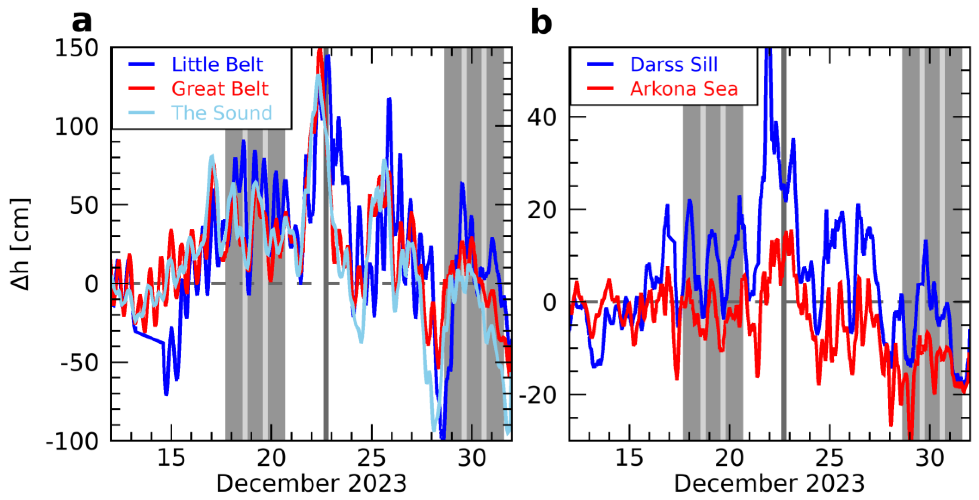
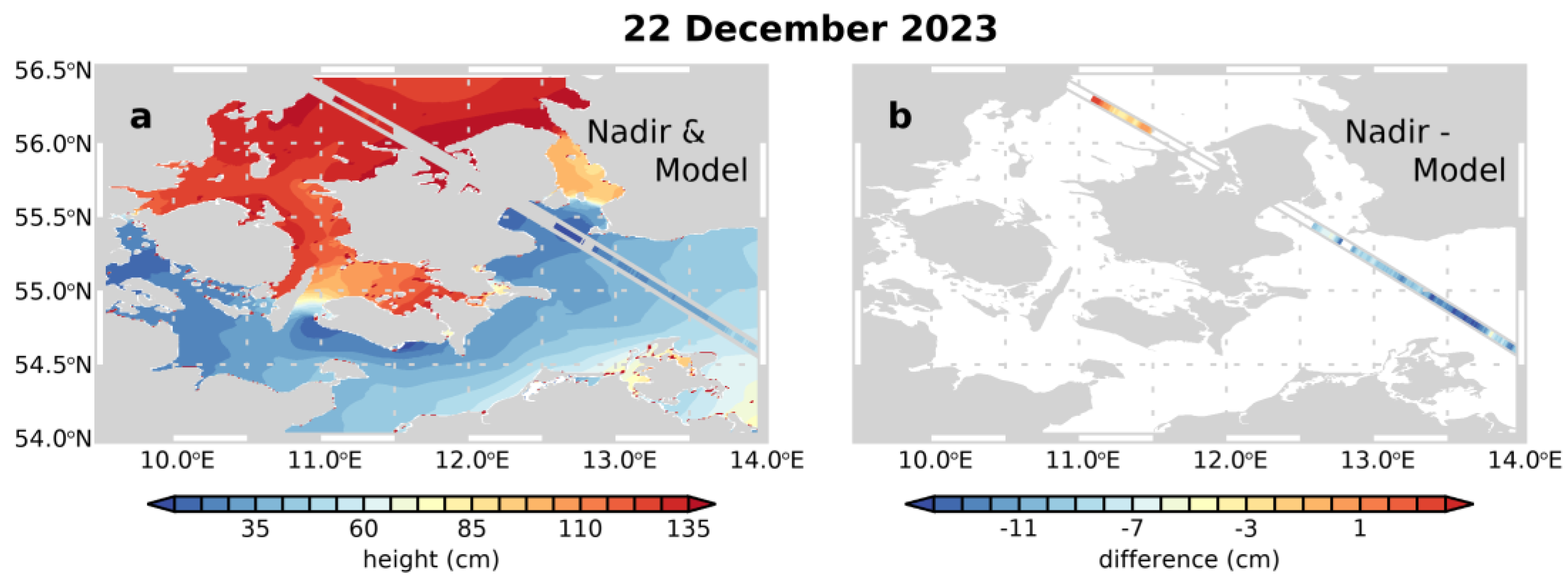
3.1. Sea-Level Signatures of the Major Baltic Inflow Event

The weather conditions leading to the moderate MBI in December 2023, as well as the corresponding volume and salt transports at Fehmarn Belt, Darss Sill and the Arkona Sea, have been described by [7]. Sea level readings from the Landsort Norra tide gauge in the Central Baltic Sea indicate that the mean Baltic sea level rose by almost 60 cm between 15 and 29 December, which corresponds to a volume increase of almost 200 km3. According to their analysis, almost 40% (75 km3) of this was salty and oxygen-rich water originating from the North Sea.
Figure 2a shows the sea level differences derived from tide gauges between the Kattegat and the Western Baltic Sea along the Danish Straits, where the flow is assumed to be hydraulically controlled [6,31]. The sea level differences (Δh) between the three Danish Straits are in good agreement, with the Great Belt and The Sound being in closer agreement than the Little Belt. On 16 December, the sea level in the north was about 30 cm higher than in the south, marking the beginning of the MBI. Maximum differences of about 150 cm occurred in all three Straits on 22 December. A second pronounced inflow event, indicated by sea level differences of up to 120 cm in the Little Belt, occurred from 25 to 27 December. On 28 December, the sea level difference changed sign again, indicating the end of the inflow from the Kattegat through the Danish Straits into the Baltic Sea. The higher-frequency signal, which is clearly distinguishable throughout the time series, is related mainly to the half-daily tides in the Kattegat.
The sea level differences (Δh) across the Western Baltic Sea at the Darss Sill and across the Arkona Sea are shown in Figure 2b. Assuming geostrophic flow, the positive south–north sea level differences correspond to eastward geostrophic currents associated with MBI events. Sea level differences near the Darss Sill reached more than 50 cm, suggesting an eastward barotropic transport from 21 to 23 December. This is consistent with observations from an autonomous offshore station at Darss Sill, which recorded the arrival of saline water on 21 December [7]. Sea level differences across the Arkona Sea reached ~30 cm on 22 and 23 December, indicating an eastward barotropic transport. However, since the Arkona Sea is much deeper and vertically stratified, barotropic transports cannot be estimated directly from the sea level differences.
A proven technique for monitoring sea level changes on spatial scales of more than 50 km is classical nadir altimetry. During the course of the MBI event, the area was overflown every day by nadir altimeters with a maximum of eight overflights on 19 and on 29 December. Figure 3a shows the instantaneous sea level SLi on 22 December as observed by the Sentinel-6 MF mission equipped with a Ku-band SAR altimeter and as simulated by the BSH-HBMnoku model. This overflight is just at the peak of the MBI event and features a strongly positive sea level in the Kattegat area and a negative between Darss Sill and Arkona Sea. The agreement between observation and model is excellent. The total along-track sea level difference from altimetry amounts to more than 130 cm. At the same time, the sea level differences observed by the tide gauges along the Danish Straits are in the range of 100–120 cm, which is in good agreement considering that the measurements are from different locations. The differences between the nadir altimetry and BSH-HBMnoku are shown in Figure 3b. The north–south sea level differences observed by the nadir altimeter are by 10 cm greater than those simulated for this extreme situation. Although the nadir measurement monitors the large-scale sea level gradient very well, it is obvious that it is not possible to obtain an insight into the flow conditions based on the 1D sea level observations alone.
In the following, we will focus on the four SWOT overflights during the course of the 2023 MBI event (cf. vertical lines in Figure 2). Two overflights took place at the beginning of the MBI event coinciding with distinct sea level gradients in the Danish Straits as observed by the tide gauges. The other two occurred at the end of the MBI event with only slightly positive sea level gradients.
The instantaneous sea level SLi derived from KaRIn and Ku-nadir for the two SWOT overflights at the beginning of the MBI event on 18 and 19 December are shown in Figure 4, together with the corresponding model data and the differences between the two datasets. While the first overflight highlights the situation in The Sound and the Arkona Sea, the second overflight is further west in the Great Belt and Darss Sill region. The extreme sea level values observed by SWOT close to the coast indicate processing errors or signal land contamination in these challenging regions.
On 18 December, the sea level gradient between Kattegat and the Western Baltic Sea builds up, and the north–south sea level difference (Δh) along The Sound is moderately positive and close to the tide gauge observations (20 cm). On 19 December, the SWOT data from both KaRIn and Ku-nadir suggest anomalous sea level differences between Kattegat and the Western Baltic Sea of ~60 cm. The corresponding BSH-HBMnoku model fields show a very similar situation, with north–south sea level differences increasing from 18 December to 19 December. However, according to the SWOT KaRIn data, the north–south sea level differences (Δh) are ~10 cm smaller than those modeled. In comparison to the model’s predictions, the SWOT observations suggest lower sea levels in the Kattegat area, higher sea levels in the northern part of the Little Belt, and a slightly stronger eastward transport over the Darss Sill.
The next available SWOT overflights are right at the end of the MBI event and cover The Sound and the Little Belt area. The SLi for the two SWOT overflights on 29 and 30 December are shown in Figure 5, together with the corresponding model data and the differences between the two datasets. For these overflights, the sea level in the Western Baltic Sea has increased by 40–60 cm and decreased by 10–20 cm in the Kattegat since the last overflights 10 days before, and the north–south sea level differences (Δh) have reversed to negative values (~−20 cm). On 29 December, both SWOT and the model suggest west–east rather than north–south sea level gradients, and sea level differences along The Sound are only slightly negative. SWOT observed lower sea levels in the Kattegat and higher levels in the Western Baltic Sea than simulated by BSH-HBMnoku. On 30 December, the sea level patterns observed by SWOT in the Little Belt area are similar to those simulated but about 5 cm higher. A notable exception is the region just south of the Little Belt, where SWOT observed lower sea levels (~5 cm) than simulated (cf. Figure 5f).

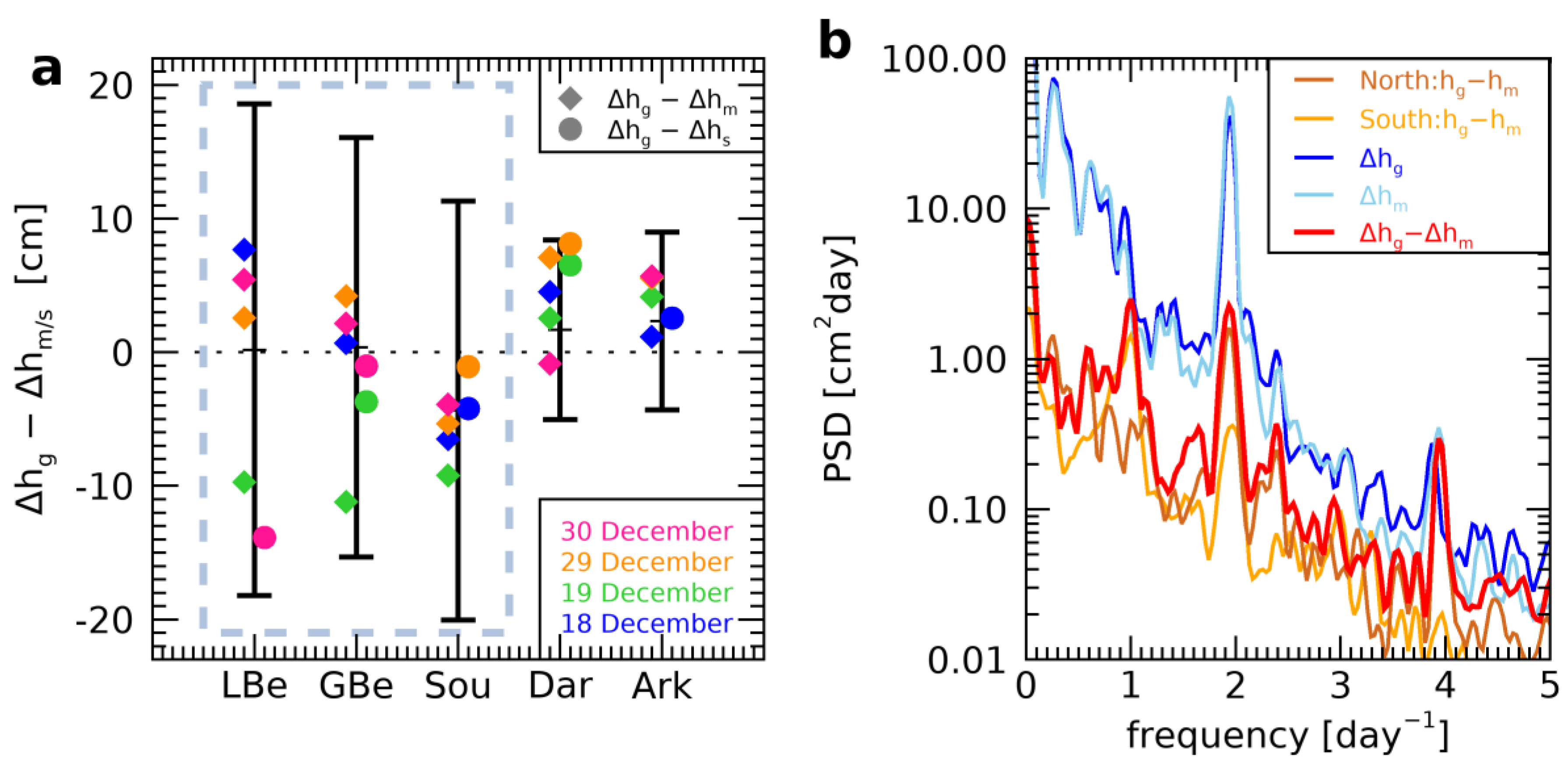
3.2. Comparison of SWOT to Nadir Altimetry Data

The analyses in Section 3 have shown the potential of SWOT to observe transient processes like the MBI event. However, on spatial scales of 50 to 200 km, there are differences of up to 10 cm between SWOT KaRIn and BSH-HBMnoku simulations. These imply differences in gradient between the Kattegat and the Western Baltic Sea, which could be used to characterize the inflow conditions. It is important to check the accuracy of the SWOT data on these scales so that they can be used to improve the model in the future. To check the consistency of the along- and across-track sea level gradients from SWOT KaRIn data and BSH-HBMnoku, we compare them to independent nadir altimetry and tide gauge data.
A direct comparison of the instantaneous sea level SLi from SWOT and nadir altimetry is complicated by the ubiquitous sea level changes between the mission overflights, which are typically hours to days apart from each other. Instead, we use SLA observations, which are referenced to the long-term mean and are dealiased for transient sea level signals of less than 20 days (ocean tides and dynamic atmospheric effects subtracted). Figure 6a,b show all SLA observations derived from KaRIn and nadir sensors for two 3-day periods at the beginning and the end of the MBI event. For both periods, SWOT KaRIn and nadir SLA agree very well with few exceptions. At the beginning of the MBI event, the SLA from SWOT KaRIn and from most nadir altimeters is about 20 cm above the long-term mean in the Kattegat and about 20 cm below in the Western Baltic Sea. At the end of the MBI event, the SLA from SWOT KaRIn is 10 to 30 cm above the mean over most of the area and close to the temporal mean in the Kattegat region. For this period, most nadir missions observe a lower SLA than SWOT KaRIn in the eastern part of the region. The cause could be either an offset in the SWOT KaRIn measurements or inaccurate regional mission biases of the respective nadir altimeters.
To further investigate the similarities and differences in the transient sea level signal captured by SWOT KaRIn and by nadir altimeters, we contrast the SLi of both altimeter datasets with the corresponding BSH-HBMnoku simulations. As a measure of the agreement between the remote sensing observations and the model, we have calculated the relative explained variance (REV, (cf. Equation (3)) by the BSH-HBMnoku for each mission separately from all overflights during December 2023. The REV values confirm the good agreement between observations and the model. The REV is 0.81 for the SWOT KaRIn mission and even higher for most of the classical nadir missions (between 0.77 and 0.94).
The SLi differences of the SWOT KaRIn and nadir versus the BSH-HBMnoku model are shown in Figure 6c,d for the same 3-day periods as before. Although the SLi can change considerably over the course of these three days, we can still investigate possible systematic differences between the model and the observations. For the first period at the beginning of the MBI event, the nadir altimeter data confirm the large-scale differences between the SWOT observations and BSH-HBMnoku. For the second period at the end of the MBI event, the agreement is very good in the Kattegat region, suggesting model deficiencies. SWOT KaRIn and nadir altimeters are less consistent in the region between Darss Sill and the Arkona Sea. It is not clear whether this is more indicative of SWOT errors or of varying model performance during the three days considered for the comparison. The prominent high track, marked with an arrow in Figure 6d, belongs to the HaiYang-2D mission, which does not provide sufficiently stable data to accurately estimate the intermission bias. A very close agreement between KaRIn and nadir data is found south of the Little Belt off the German coast. This suggests that the local dynamics (e.g., related to wind surge or flow along the Little Belt) are not adequately simulated.

4. Discussion

Comparison of tide gauges and altimeters is an established technique for estimating the accuracy of remote sensing measurements [13,34,35]. Unfortunately, for this study, a sound comparison between these two datasets is hampered by the very limited SWOT overflights close to the tide gauges during the MBI event. Instead, we examine the characteristic differences between tide gauge readings and model simulations, with a focus on the north–south SLi differences. The derived statistical values are compared with the differences between tide gauge and the SWOT KaRIn observations.
The tide gauge observations and the BSH-HBMnoku simulations are in very good agreement. The REV value by BSH-HBMnoku at the tide gauges is between 0.92 and 0.97 in December 2023. The north–south sea level difference (Δh) along the Danish Straits and at Darss Sill is captured very well by the model but less well in the Arkona Sea. For the Danish Straits and Darss Sill, the REV value of Δh is 0.94 to 0.95, and for the Arkona Sea it is 0.81..
The mean and 2 σ range of the difference Δhgauge − Δhmodel is shown in Figure 7a for the Danish Straits, Darss Sill and Arkona Sea. The corresponding Δhgauge − Δhmodel and Δhgauge − Δhswot differences are indicated by diamonds and circles, respectively. The mean offset of Δhgauge − Δhmodel is close to zero for the Little Belt and the Great Belt. The offset amounts to about 2 cm for Darss Sill and the Arkona Sea, but these values are not statistically significant. The offset for The Sound is −4.4 ± 3.4 cm. This offset is dominated by a model level 5.5 cm higher than the tide gauge readings at the Viken station in the Kattegat. A probable cause may be an inconsistent vertical datum of the Viken station. The Swedish tide gauges are subject to the Fennoscandian uplift. As the vertical rates are not known with sufficient accuracy for each station, we have not corrected for this effect, but they may well amount to a 5 cm correction relative to the BSCD2000 [36]. The Δhgauge − Δhswot differences are within the 2σ range of the Δhgauge − Δhmodel differences and are close to each other in most cases. Exceptions are the Great Belt on 19 December and the Little Belt on 30 December. On 19 December, the sea level gradient along all Danish Straits seems to be overestimated by the model. On 30 December, the high levels recorded by SWOT in the northern part of the Little Belt are probably not realistic.
Even though the agreement between the model and the tide gauges is already excellent, we further study the spectral differences between the tide gauges in the Danish Straits and BSH-HBMnoku. The power spectrum of the north–south height differences Δhgauge, Δhmodel and Δhgauge − Δhmodel in the Danish Straits is shown in Figure 7b. The model deviates from the tide gauges mainly in the half-daily and daily bands. An analysis of the height differences shows that the differences in the Kattegat (North) are mainly in the half-daily band, while the differences in the Western Baltic Sea are mainly in the daily band. This suggests that the quarter- and half-daily ocean tides in the BSH-HBMnoku model could be further improved in the Kattegat region, as already discussed by [9]. The energy in the daily band originates from the Western Baltic Sea and is most likely related to deficiencies in the modeling of Baltic seiches, which have periods of 23 to 27 h in this region [15,37,38].

5. Conclusions

The recently launched SWOT mission provides a new set of spatial sea level observations for small-scale studies. During the course of the moderate MBI event in December 2023, there were six SWOT overflights in the Kattegat–Western Baltic Sea area. Unfortunately, the KaRIn data are not available for two overflights, and the maximum of the MBI event was not covered. Nevertheless, there are two snapshots showing the large-scale sea level gradients at the beginning of MBI event and two right at the end, which exhibit the sea level patterns related to the concurrent moderate MBI event in December 2023 with unprecedented detail.
In general, MBI events can only be monitored by sparsely distributed tide gauges and by salinity and ocean current measurements at a few moorings [4,7]. Large-scale altimetry has previously been used to study the occurrence of MBI events [39]. However, as far as we are aware, high-rate nadir altimetry has not yet been used for observing MBI events. With ten active nadir altimetry missions currently in orbit, the area is covered by a total of 65 overflights, allowing the monitoring of the dominant flow processes in the area [40] and providing additional information for spatial scales larger than 50 km. On 22 December, during the maximum sea level gradients in the Danish Straits, Sentinel-6 MF observed a large-scale sea level difference of more than 130 cm between the western Kattegat and the western Arkona Sea, which is almost 10% larger than simulated. However, not all missions provide stable and valid data in coastal regions, and the spatial resolution of the 1D sea level measurements is not sufficient to resolve and understand the transient processes in this area [14,31]. The good agreement between the nadir and SWOT KaRIn altimetry provides confidence in the KaRIn data, especially considering that the observations may be separated by up to two days. Finally, tide gauge data can be used to detect unreliable SWOT KaRIn data.
SWOT KaRIn observations and the simulations with the regional 3D BSH-HBMnoku ocean circulation model are in good agreement for most aspects. Currently, BSH-HBMnoko is already able to explain 80% of the SWOT KaRIn data variance. However, there are differences between the two on spatial scales of 50 to 200 km, which appear to be related to model deficiencies on daily to sub-daily time scales. In addition, the SWOT data have many fine-scale structures like eddies and fronts that are not adequately modeled. The validation of these features is beyond the scope of this study, but the features appear to be plausible. This study shows that SWOT KaRIn altimetry provides valuable additional information about the transient processes in the region. Although the 2023 MBI event was only moderate, the underlying processes are the same as for very strong MBI events. The temporal sampling rate is not adequate for the process under consideration, but the SWOT observations together with high-rate nadir altimetry can significantly improve the existing in situ monitoring and open up the prospect of improving the model predictions by assimilating this novel data.

Author Contributions

Conceptualization, S.E., H.D. and T.S.; methodology, S.E. and T.S.; software, S.E. and T.S.; data curation, S.E., T.S. and R.S.; writing—original draft preparation, S.E.; writing—review and editing, S.E., T.S., H.D. and R.S.; visualization, S.E. All authors have read and agreed to the published version of the manuscript.

Funding

RS acknowledges funding by the TIDUS project within the NEROGRAV research unit (DFG Research Unit 2736, Grant: TH864/15-2).

Data Availability Statement

The SWOT L2_LR_SSH data are provided by the SWOT project, 2023. SWOT Level-2 KaRIn Low Rate SSH Expert (v2.0) is available at. https://doi.org/10.24400/527896/A01-2023.015 (accesssed on 1 December 2024). High-rate Level 2 nadir altimetry data from the Cryosat-2, Saral, Sentinel-3A, Sentinel-3B, Jason-3, Sentinel-6 MF, HaiYang-2B, HaiYang-2C, HaiYang-2D and the SWOT mission are corrected and processed within GFZ’s Altimeter Data System ADS. The high-rate instantaneous sea level and Sea Level Anomaly data from nadir altimetry processed by GFZ’s ADS and used for this study can be provided upon request by the authors. The Level 2 GDR-F altimeter products of Saral, Jason-3 and SWOT nadir were produced and distributed by Aviso+ (https://www.aviso.altimetry.fr/, accessed on 1 December 2024), as part of the Ssalto ground processing segment. The paper contains modified Copernicus Sentinel data for Sentinel-3A and Sentinel-3B (https://dataspace.copernicus.eu/explore-data/data-collections/sentinel-data/sentinel-3, accessed on 1 December 2024), SRAL, Level 2 Marine, No-Time-Critical (NTC), baseline 52, and for Sentinel-6 MF (https://user.eumetsat.int/data-access, accessed on 1 December 2024), Level 2, High-Resolution (HR) Non-Time-Critical (NTC), baseline F08. Cryosat-2 L2 NOP-IOP-GOP SAR data, Version Baseline D is available at: https://doi.org/10.5270/CR2-pbm8gdx (accessed on 1 December 2024). Level 2 SDR data from China’s ocean satellites HaiYang-2B/C/D were obtained from https://osdds.nsoas.org.cn (accessed on 1 December 2024). The tide gauge data were collated within the Copernicus Marine Service (in situ) and EMODnet collaboration framework. “Baltic Sea—near real-time (NRT) in situ quality controlled observations” (https://doi.org/10.48670/moi-00032, accessed on 10 February 2025) are made freely available by the E.U. Copernicus Marine Service (CMEMS) and the programs that contribute to it.. The BSH-HBMnoku model data “Modellierte Wasserstandsauslenkung des operationellen Zirkulationsmodells des BSH in der deutschen Bucht und der westlichen Ostsee (horizontale Auflösung ca. 900 m) 2023 - Serie” is freely available from the German Federal Maritime and Hydrographic Agency (BSH) at https://data.bsh.de/OpenData/OperationalModel/ (accessed on 1 December 2024). Data analysis and plotting was performed in Interactive Data Language (IDL9.01) software available from NV5 Geospatial (https://www.nv5geospatialsoftware.com/Products/IDL, accessed on 1 December 2024).

Acknowledgments

We thank Joachim Schwabe (BKG Leipzig/Germany) for his most valuable help with tide gauge datum issues, Swantje Bastin (BSH Hamburg/Germany) for providing information about the BSH-HBMnoku vertical reference and Mira Esselborn for her support in creating the graphical abstract. The authors would like to thank AVISO, CNES, ESA, EUMETSAT, NASA and NOAA for providing high-quality GDR data for Cryosat-2, Saral, Jason-3, SWOT, Sentinel-3A/B and Sentinel-6 MF and NSOAS for producing and providing the HaiYang-2 Level 2 altimeter SDR data free of charge.

Conflicts of Interest

The authors declare no conflicts of interest. The funders had no role in the design of the study; in the collection, analyses, or interpretation of data; in the writing of the manuscript; or in the decision to publish the results.

Abbreviations

The following abbreviations are used in this manuscript:
GDRGeophysical Data Record
HBMHigh-Resolution Model for the Baltic Sea—Baltic Operational Oceanography System
KaRInKa-band Radar Interferometer
MBIMajor Baltic Inflow
REVRelative Explained Variance
SARSynthetic Aperture Radar
SLASea Level Anomaly
SLiInstantaneous Sea Level
SWOTSurface Water and Ocean Topography Mission

References

  1. Weisse, R.; Dailidiene, I.; Hünicke, B.; Kahma, K.; Madsen, K.; Omstedt, A.; Parnell, K.; Schöne, T.; Soomere, T.; Zhang, W.; et al. Sea Level Dynamics and Coastal Erosion in the Baltic Sea Region. Earth Syst. Dyn. 2021, 12, 871–898. [Google Scholar] [CrossRef]
  2. Lehmann, A.; Myrberg, K.; Post, P.; Chubarenko, I.; Dailidiene, I.; Hinrichsen, H.-H.; Hüssy, K.; Liblik, T.; Meier, H.E.M.; Lips, U.; et al. Salinity Dynamics of the Baltic Sea. Earth Syst. Dyn. 2022, 13, 373–392. [Google Scholar] [CrossRef]
  3. Lass, H.U.; Matthäus, W. On Temporal Wind Variations Forcing Salt Water Inflows into the Baltic Sea. Tellus A Dyn. Meteorol. Oceanogr. 1996, 48, 663–671. [Google Scholar] [CrossRef]
  4. Mohrholz, V. Major Baltic Inflow Statistics–Revised. Front. Mar. Sci. 2018, 5, 384. [Google Scholar] [CrossRef]
  5. Mohrholz, V.; Naumann, M.; Nausch, G.; Krüger, S.; Gräwe, U. Fresh Oxygen for the Baltic Sea—An Exceptional Saline Inflow after a Decade of Stagnation. J. Mar. Syst. 2015, 148, 152–166. [Google Scholar] [CrossRef]
  6. Stanev, E.V.; Pein, J.; Grashorn, S.; Zhang, Y.; Schrum, C. Dynamics of the Baltic Sea Straits via Numerical Simulation of Exchange Flows. Ocean Model. 2018, 131, 40–58. [Google Scholar] [CrossRef]
  7. Purkiani, K.; Jochumsen, K.; Fischer, J.-G. Observation of a Moderate Major Baltic Sea Inflow in December 2023. Sci. Rep. 2024, 14, 16577. [Google Scholar] [CrossRef]
  8. Pham, N.T.; Staneva, J.; Bonaduce, A.; Stanev, E.V.; Grayek, S. Interannual Sea Level Variability in the North and Baltic Seas and Net Flux through the Danish Straits. Ocean Dyn. 2024, 74, 669–684. [Google Scholar] [CrossRef]
  9. Brüning, T.; Li, X.; Schwichtenberg, F.; Lorkowski, I. An Operational, Assimilative Model System for Hydrodynamic and Biogeochemical Applications for German Coastal Waters. Hydrogr. Nachrichten 2021, 118, 6–15. [Google Scholar] [CrossRef]
  10. Abdalla, S.; Kolahchi, A.A.; Adusumilli, S.; Bhowmick, S.A.; Alou-Font, E.; Amarouche, L.; Andersen, O.B.; Antich, H.; Aouf, L.; Arbic, B.; et al. Altimetry for the Future: Building on 25 Years of Progress. Adv. Space Res. 2021, 68, 319–363. [Google Scholar] [CrossRef]
  11. Cipollini, P.; Calafat, F.M.; Jevrejeva, S.; Melet, A.; Prandi, P. Monitoring Sea Level in the Coastal Zone with Satellite Altimetry and Tide Gauges. Surv. Geophys. 2017, 38, 33–57. [Google Scholar] [CrossRef] [PubMed]
  12. Vignudelli, S.; Birol, F.; Benveniste, J.; Fu, L.-L.; Picot, N.; Raynal, M.; Roinard, H. Satellite Altimetry Measurements of Sea Level in the Coastal Zone. Surv. Geophys. 2019, 40, 1319–1349. [Google Scholar] [CrossRef]
  13. Esselborn, S.; Schöne, T.; Illigner, J.; Weiß, R.; Artz, T.; Huang, X. Validation of Recent Altimeter Missions at Non-Dedicated Tide Gauge Stations in the Southeastern North Sea. Remote Sens. 2022, 14, 236. [Google Scholar] [CrossRef]
  14. Pujol, M.-I.; Dupuy, S.; Vergara, O.; Román, A.S.; Faugère, Y.; Prandi, P.; Dabat, M.-L.; Dagneaux, Q.; Lievin, M.; Cadier, E.; et al. Refining the Resolution of DUACS Along-Track Level-3 Sea Level Altimetry Products. Remote Sens. 2023, 15, 793. [Google Scholar] [CrossRef]
  15. Metzner, M.; Gade, M.; Hennings, I.; Rabinovich, A.B. The Observation of Seiches in the Baltic Sea Using a Multi Data Set of Water Levels. J. Mar. Syst. 2000, 24, 67–84. [Google Scholar] [CrossRef]
  16. Liebsch, G.; Novotny, K.; Dietrich, R.; Shum, C.K. Comparison of Multimission Altimetric Sea-Surface Heights with Tide Gauge Observations in the Southern Baltic Sea. Mar. Geod. 2002, 25, 213–234. [Google Scholar] [CrossRef]
  17. Madsen, K.S.; Høyer, J.L.; Tscherning, C.C. Near-Coastal Satellite Altimetry: Sea Surface Height Variability in the North Sea–Baltic Sea Area. Geophys. Res. Lett. 2007, 34, L14601. [Google Scholar] [CrossRef]
  18. Madsen, K.S.; Høyer, J.L.; Suursaar, Ü.; She, J.; Knudsen, P. Sea Level Trends and Variability of the Baltic Sea From 2D Statistical Reconstruction and Altimetry. Front. Earth Sci. 2019, 7, 243. [Google Scholar] [CrossRef]
  19. Passaro, M.; Müller, F.L.; Oelsmann, J.; Rautiainen, L.; Dettmering, D.; Hart-Davis, M.G.; Abulaitijiang, A.; Andersen, O.B.; Høyer, J.L.; Madsen, K.S.; et al. Absolute Baltic Sea Level Trends in the Satellite Altimetry Era: A Revisit. Front. Mar. Sci. 2021, 8, 647607. [Google Scholar] [CrossRef]
  20. Elken, J.; Barzandeh, A.; Maljutenko, I.; Rikka, S. Reconstruction of Baltic Gridded Sea Levels from Tide Gauge and Altimetry Observations Using Spatiotemporal Statistics from Reanalysis. Remote Sens. 2024, 16, 2702. [Google Scholar] [CrossRef]
  21. Fu, L.-L.; Pavelsky, T.; Cretaux, J.-F.; Morrow, R.; Farrar, J.T.; Vaze, P.; Sengenes, P.; Vinogradova-Shiffer, N.; Sylvestre-Baron, A.; Picot, N.; et al. The Surface Water and Ocean Topography Mission: A Breakthrough in Radar Remote Sensing of the Ocean and Land Surface Water. Geophys. Res. Lett. 2024, 51, e2023GL107652. [Google Scholar] [CrossRef]
  22. SWOT Project, SWOT Level-2 KaRIn Low Rate SSH Expert (v2.0), 2024, CNES. Available online: https://www.aviso.altimetry.fr/en/data/products/sea-surface-height-products/global/swot-karin-low-rate-ocean-products.html (accessed on 1 December 2024).
  23. Schöne, T.; Esselborn, S.; Rudenko, S.; Raimondo, J.-C. Radar Altimetry Derived Sea Level Anomalies—The Benefit of New Orbits and Harmonization. In System Earth via Geodetic-Geophysical Space Techniques; Flechtner, F.M., Gruber, T., Güntner, A., Mandea, M., Rothacher, M., Schöne, T., Wickert, J., Eds.; Springer: Berlin/Heidelberg, Germany, 2010; pp. 317–324. ISBN 978-3-642-10227-1. [Google Scholar]
  24. Dach, R.; Schaer, S.; Arnold, D.; Kalarus, M.S.; Prange, L.; Stebler, P.; Villiger, A.; Jäggi, A. CODE Final Product Series for the IGS. In Dach Rolf Schaer Stefan Arnold Daniel Kalarus Maciej Sebastian Prange Lars Stebler Pascal Villiger Arturo Jäggi Adrian 2020 CODE Final Prod. Ser. IGS Datensatz Astron; The University of Bern: Bern, Switzerland, 2020. [Google Scholar]
  25. Petit, G.; Luzum, B. IERS Conventions (2010); IERS Technical Note; Verlag des Bundesamts für Kartographie und Geodäsie: Frankfurt am Main, Germany, 2010; p. 179. ISBN 3-89888-989-6. [Google Scholar]
  26. Desai, S.; Wahr, J.; Beckley, B. Revisiting the Pole Tide for and from Satellite Altimetry. J. Geod. 2015, 89, 1233–1243. [Google Scholar] [CrossRef]
  27. Lyard, F.H.; Allain, D.J.; Cancet, M.; Carrère, L.; Picot, N. FES2014 Global Ocean Tide Atlas: Design and Performance. Ocean Sci. 2021, 17, 615–649. [Google Scholar] [CrossRef]
  28. Schaeffer, P.; Pujol, M.-I.; Veillard, P.; Faugere, Y.; Dagneaux, Q.; Dibarboure, G.; Picot, N. The CNES CLS 2022 Mean Sea Surface: Short Wavelength Improvements from CryoSat-2 and SARAL/AltiKa High-Sampled Altimeter Data. Remote Sens. 2023, 15, 2910. [Google Scholar] [CrossRef]
  29. Jousset, S.; Mulet, S.; Greiner, E.; Wilkin, J.; Vidar, L.; Dibarboure, G.; Picot, N. New Global Mean Dynamic Topography CNES-CLS-22 Combining Drifters, Hydrological Profiles and High Frequency Radar Data. ESS Open Arch. 2023, preprint. [Google Scholar] [CrossRef]
  30. Carrère, L.; Lyard, F. Modeling the Barotropic Response of the Global Ocean to Atmospheric Wind and Pressure Forcing-Comparisons with Observations. Geophys. Res. Lett. 2003, 30, 1275. [Google Scholar] [CrossRef]
  31. Omstedt, A.; Elken, J.; Lehmann, A.; Leppäranta, M.; Meier, H.E.M.; Myrberg, K.; Rutgersson, A. Progress in Physical Oceanography of the Baltic Sea during the 2003–2014 Period. Prog. Oceanogr. 2014, 128, 139–171. [Google Scholar] [CrossRef]
  32. Le Traon, P.Y.; Reppucci, A.; Alvarez Fanjul, E.; Aouf, L.; Behrens, A.; Belmonte, M.; Bentamy, A.; Bertino, L.; Brando, V.E.; Kreiner, M.B.; et al. From Observation to Information and Users: The Copernicus Marine Service Perspective. Front. Mar. Sci. 2019, 6, 234. [Google Scholar] [CrossRef]
  33. Schwabe, J.; Ågren, J.; Liebsch, G.; Westfeld, P.; Hammarklint, T.; Mononen, J.; Andersen, O.B. The Baltic Sea Chart Datum 2000 (BSCD2000): Implementation of a Common Reference Level in the Baltic Sea. Int. Hydrogr. Rev. 2020, 23, 63–82. [Google Scholar]
  34. Mitchum, G.T. Comparison of TOPEX Sea Surface Heights and Tide Gauge Sea Levels. J. Geophys. Res. Oceans 1994, 99, 24541–24553. [Google Scholar] [CrossRef]
  35. Fenoglio-Marc, L.; Schöne, T.; Illigner, J.; Becker, M.; Manurung, P. Khafid Sea Level Change and Vertical Motion from Satellite Altimetry, Tide Gauges and GPS in the Indonesian Region. Mar. Geod. 2012, 35, 137–150. [Google Scholar] [CrossRef]
  36. Männel, B.; Schöne, T.; Bradke, M.; Schuh, H. Vertical Land Motion at Tide Gauges Observed by GNSS: A New GFZ-TIGA Solution. In Geodesy for a Sustainable Earth: Proceedings of the 2021 Scientific Assembly of the International Association of Geodesy, Beijing, China, 28 June–2 July 2021; Freymueller, J.T., Sánchez, L., Eds.; Springer International Publishing: Cham, Switzerland, 2023; pp. 279–287. [Google Scholar] [CrossRef]
  37. Lorenz, M.; Viigand, K.; Gräwe, U. Untangling the Waves: Decomposing Extreme Sea Levels in a Non-Tidal Basin, the Baltic Sea. Nat. Hazards Earth Syst. Sci. 2024; preprint. [Google Scholar] [CrossRef]
  38. Jönsson, B.; Döös, K.; Nycander, J.; Lundberg, P. Standing Waves in the Gulf of Finland and Their Relationship to the Basin-Wide Baltic Seiches. J. Geophys. Res. Oceans 2008, 113, C03004. [Google Scholar] [CrossRef]
  39. Stramska, M.; Aniskiewicz, P. Satellite Remote Sensing Signatures of the Major Baltic Inflows. Remote Sens. 2019, 11, 954. [Google Scholar] [CrossRef]
  40. Elyouncha, A.; Broström, G.; Johnsen, H. Synergistic Utilization of Spaceborne SAR Observations for Monitoring the Baltic Sea Flow Through the Danish Straits. Earth Space Sci. 2024, 11, e2024EA003794. [Google Scholar] [CrossRef]
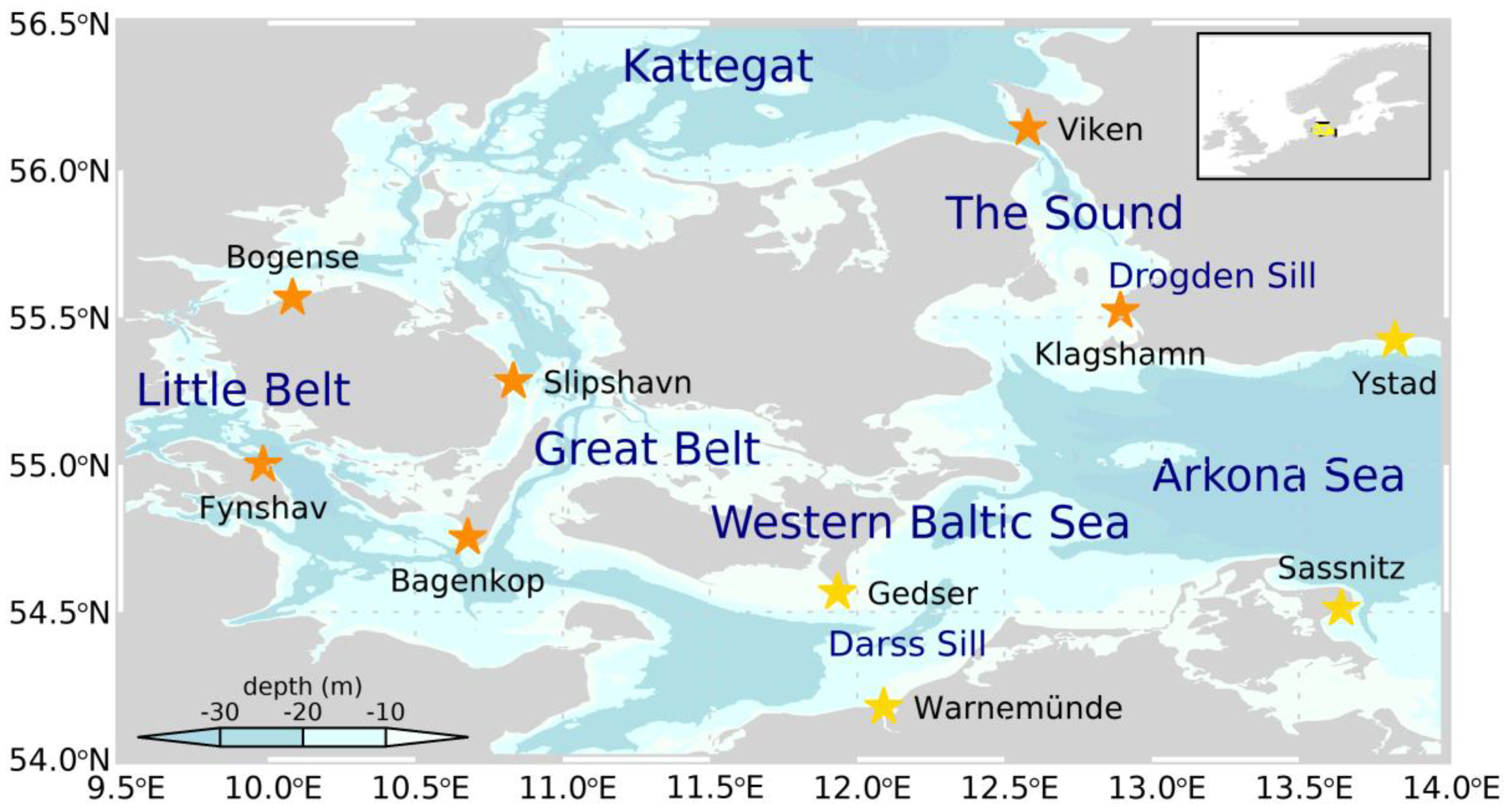
Figure 1. Map showing the geographical terms used in this paper. The Danish Straits include Little Belt, Great Belt and The Sound. Tide gauges in the Danish Straits are shown in orange, and those in the Western Baltic Sea are shown in yellow.
Remotesensing 17 01289 g001
Figure 2. Sea level difference (Δh) based on tide gauges: (a) hNorth-hSouth along the Danish Straits, where positive values imply transport to the south. (b) hSouth-hNorth across the Western Baltic Sea near Darss Sill and across the Arkona Sea, where positive differences imply barotropic transport to the East. The time series are 3 h boxcar-filtered. SWOT overflights are indicated by light gray vertical lines, the Sentinel-6 MF overflight is indicated by a gray vertical line, and periods where nadir altimetry compared with SWOT overflights are shaded gray.
Remotesensing 17 01289 g002
Figure 3. (a) Instantaneous sea level (SLi) on 22 December 2023 17:05 UTC observed by Sentinel-6 MF nadir altimetry and simulated by the BSH-HBMnoku model. (b) Sea level differences between nadir altimetry and model.
Remotesensing 17 01289 g003
Figure 4. Instantaneous sea level (SLi) (a,d) from SWOT (KaRIn and nadir) measurements, (b,e) from the BSH-HBMnoku model, and (c,f) difference SWOT minus BSH-HBMnoku (ac) on 18 December 2023 16:26 UTC (df) and 19 December 2023 16:27 UTC.
Remotesensing 17 01289 g004
Figure 5. Instantaneous sea level (SLi) (a,d) from SWOT (KaRIn and nadir) measurements, (b,e) from the BSH-HBMnoku model, and (c,f) difference in SWOT minus BSH-HBMnoku (ac) on 29 December 2023 14:49 UTC (df) and 30 December 2023 14:50 UTC.
Remotesensing 17 01289 g005
Figure 6. (a,b) Sea level anomalies (SLA) from SWOT KaRIn and all available nadir altimetry for two 3-day periods: (a) inflow (17–20 December 2023 16:30 UTC) and (b) post-inflow (28–31 December 2023 14:50 UTC). (c,d) Difference in instantaneous sea level (SLi) from altimetry (all nadir and SWOT KaRIn) vs. BSH-HBMnoku model for (c) inflow and (d) post-inflow. Tide gauge locations are indicated by green stars, an exceptionally high HaiYang-2D track by a black arrow.
Remotesensing 17 01289 g006
Figure 7. Comparison of the north–south height difference (Δh) from the gauge, model and SWOT. (a) Mean and 2σ range of Δhgauge − Δhmodel in December 2003 for Little Belt (LBe), Great Belt (GBe), The Sound (Sou), Darss Sill (Dar) and Arkona Sea (Ark). Symbols show the values during SWOT overflights, diamonds for Δhgauge − Δhmodel, and circles for Δhgauge − Δhswot. Overflights are color-coded. The gray stitched box marks the data from the Danish Straits used for the power spectra. (b) Power spectral density averaged over the three Danish Straits. Spectra of Δh from gauges (blue), the model (light blue) and Δhgauge − Δhmodel (red), and gauge–model height difference in the North (brown) and in the South (orange).
Remotesensing 17 01289 g007
Table 2. List of the tide gauges used for the three Danish Straits and across the Darss Sill and the Arkona Sea. The northern gauges are in the first row, and the southern in the second.
Little BeltGreat BeltThe Sound Darss SillArkona Sea
BogenseSlipshavnVikenGedserYstad
FynshavBagenkopKlagshamnWarnemündeSassnitz
Disclaimer/Publisher’s Note: The statements, opinions and data contained in all publications are solely those of the individual author(s) and contributor(s) and not of MDPI and/or the editor(s). MDPI and/or the editor(s) disclaim responsibility for any injury to people or property resulting from any ideas, methods, instructions or products referred to in the content.

