Expansion of Output Spatial Extent in the Wavenumber Domain Algorithms for Near-Field 3-D MIMO Radar Imaging

Abstract

Microwave camera provides 3-D high-resolution radar images at video frame rates, enabling the capture of dynamic target features. Multiple-input–multiple-output (MIMO) array-based 3-D radar imaging system requires fewer antennas, which effectively reduces hardware costs. Due to the limited computational resources of the miniaturized MIMO microwave camera, real-time processing of a large amount of 3-D echo data requires an imaging algorithm that has both real-time performance and large output spatial extent. This paper presents the limited output spatial extent and spatial aliasing in existing MIMO wavenumber domain algorithms through theoretical derivation and simulation. To suppress aliasing while expanding the output spatial extent, an optimization approach for the wavenumber domain algorithms is proposed. The improved wavenumber domain algorithms divide the target area into multiple sub-blocks, and a broader range of imaging results is obtained through independent imaging of the sub-blocks and a spatial aliasing suppression filter. Simulation results show that the improved wavenumber domain algorithms effectively suppress the aliasing energy of each sub-block while maintaining the advantage of low time complexity. Expansion of output spatial extent in existing MIMO wavenumber domain algorithms is achieved.

1. Introduction

Near-field microwave imaging technology demonstrates significant target penetration capabilities and robust environmental adaptability, making it advantageous in applications such as concealed objects detection [1,2,3], medical diagnostics [4], and human-machine interaction [5]. Among various near-field 3-D imaging systems, microwave camera [6] provides high resolution radar images at video frame rates, capturing the dynamic scattering characteristics of targets and addressing the growing demand for real-time detection. Nevertheless, video frame rates radar imaging requires systems with ultrahigh echo processing capabilities, which imposes rigorous requirements on both the architectural design of radar systems and the computational efficiency of imaging algorithms.

Near-field imaging radar systems typically use wideband illumination and 2-D apertures to achieve the range resolution and the cross-range resolution, respectively. Traditional 3-D imaging systems achieve cross-range resolution with 2-D transceiver arrays [7,8,9]. To avoid wavenumber spectrum aliasing caused by spatial undersampling, such systems require an extremely large number of antenna elements and corresponding hardware resources, which results in very high system costs.

The transmit and receive arrays of MIMO radar form larger virtual arrays through spatial convolution, effectively reducing the number of elements required by the system [10,11]. MIMO-Synthetic Aperture Radar (SAR) and 2-D MIMO arrays are two widely researched near-field 3-D microwave imaging systems. MIMO-SAR [12,13,14,15] combines 1-D MIMO arrays with synthetic aperture technology to achieve cross-range resolution, requiring fewer antennas. However, synthetic aperture requires the 1-D array to scan along the height direction, and the time consumption associated with motion limits the efficiency of imaging sampling. Two-D MIMO [16,17,18,19] forms cross-range virtual apertures through spatial convolution, requiring moderate element consumption. The imaging sampling process does not require relative motion between the array and the targets, making it better suited for microwave cameras. With the development of metasurface technology, the complexity and cost of 2-D MIMO arrays will be further reduced [20]. The cross MIMO array, a 2-D MIMO configuration with transmitters and receivers uniformly distributed along the azimuth and height directions, respectively, exhibits non-sparsity and wide wavenumber coverage [21]. Accordingly, the subsequent discussion on 3-D MIMO imaging algorithms focuses on the cross-MIMO array.

MIMO radar 3-D imaging algorithms can be categorized into time domain and wavenumber domain methods. The back-projection algorithm (BPA), commonly used in SAR [22,23], reconstructs images by coherently accumulating echo signals. With the precise calculation of distances between transceivers and grid points, BPA is applicable to most MIMO array configurations [24]. Moreover, the image reconstruction extent of BPA can also be freely selected based on the definition of the grid coordinates. Kirchhoff Migration Algorithm (KMA) describes image reconstruction with the wave equations [25]. The modified version, MKMA [26] has been widely used in 3-D MIMO radar imaging. As a time-domain imaging algorithm, MKMA is similarly compatible with most MIMO array configurations. However, due to the large volume of echo data in the MIMO radar 3-D imaging system, the time complexity of BPA and KMA is $O\left(N^5\right)$. This poses challenges in meeting the real-time requirements of microwave camera systems with limited computational resources. Fast-factorized BPA and KMA [27,28] reduce the time complexity to $O\left(N^3{log}_{2}N\right)$ through sub-aperture partitioning and iterative processing. However, the errors generated during aperture fusion increase as the number of sub-apertures, resulting in a deterioration of reconstruction quality.

In near-field imaging scenarios, the errors induced by approximating equivalent phase center for transceivers are significant, thus algorithms such as Range-Doppler, Chirp-Scaling, and $\omega -K$ cannot be directly applied to MIMO radar imaging. Range Migration Algorithm (RMA) compensates for the wavefront curvature in the wavenumber domain through Stolt interpolation. It is an extension of the $\omega -K$ algorithm from SAR imaging to MIMO radar 3-D imaging [29]. Paraxial-RMA [30] and Cross-RMA [31] are adaptations of RMA for cross MIMO arrays. Paraxial-RMA simplifies the decoupling between wavenumber variables and spatial coordinates variables using the paraxial approximation, effectively reducing the time complexity to $O\left(N^3{log}_{2}N\right)$. However, as the azimuth and height angles increase, the errors from paraxial approximation become more pronounced, leading to a defocusing problem and degrading imaging quality. Cross-RMA obtains an accurate reconstruction solution closely resembling that of the BPA by combining variable substitution, Stolt interpolation, and coherent summation. As a cost, the time complexity increases to $O\left(N^4{log}_{2}N\right)$. Phase Shift Migration Algorithm (PSMA) is another wavenumber domain algorithm [32] for MIMO radar 3-D imaging. It performs wavefront correction and focusing in the distance direction by independently summing over each range plane. Compared to RMA, PSMA avoids the interpolation error, achieving a higher reconstruction accuracy, though with a time complexity of $O\left(N^4{log}_{2}N\right)$. Similar to PSMA, the Fast Wavenumber Domain 3-D Near-Field Imaging Algorithm [33] also uses coherent summation for wavefront correction and focusing in the distance direction. However, the distance approximation leads to a decrease in reconstruction accuracy, and a time complexity of $O\left(N^4{log}_{2}N\right)$ does not offer a significant advantage.

As mentioned above, time domain algorithms offer flexibility in adjusting the image reconstruction extent, but they come with higher time complexity. In contrast, the wavenumber domain algorithms typically have lower time complexity, making them more suitable for microwave cameras with limited computational resources. However, the azimuth and height dimension focusing process in the wavenumber domain algorithms requires Fourier and inverse Fourier transforms. The output spatial extent is limited to the physical aperture coverage of the 2-D MIMO array. Nevertheless, the Unambiguous Sampling Range (USR) is determined by both the antenna spacing and the wavenumber angular range. When USR exceeds the physical aperture, existing MIMO wavenumber domain algorithms are unable to correctly reconstruct scattering information. To address this, this paper proposes a method to expand the output spatial extent. It retains the advantage of the low time complexity of the wavenumber domain algorithms while achieving an extended output spatial extent in azimuth and height dimensions. The innovative contributions of this work are as follows:

• A method for adjusting the central output image in existing wavenumber domain algorithms is proposed.
• The spatial aliasing phenomenon in existing wavenumber domain algorithms is analyzed, and an algorithm for suppression is designed.
• An approach for expanding output spatial extent in existing wavenumber domain algorithms is proposed while preserving the advantage of low computational complexity.

The rest of this article is organized as follows. Section 2 introduces the imaging geometry of the 2-D MIMO array and theoretically calculates the output spatial extent of existing MIMO wavenumber domain algorithms. For targets within USR, the spatial aliasing phenomena in the output image are derived. Section 3 presents the implementation procedures of the sub-block imaging algorithm and the spatial aliasing filter. Time complexities of the algorithms are also provided in Section 3. Section 4 presents the simulation results. Section 5 summarizes the results and concludes this paper.

2. Imaging Model and Spatial Aliasing

2.1. Imaging Model

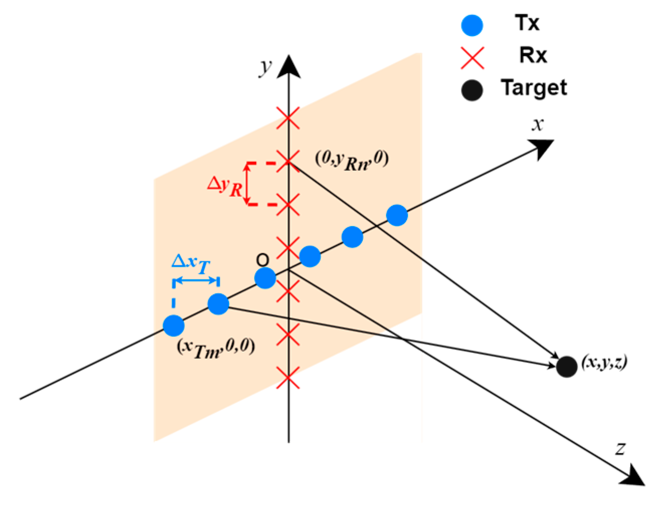
Two-D cross MIMO array consists of $N_T$ transmitters and $N_R$ receivers, with coordinates $\left(x_{Tm},\mathrm{0,0}\right)$ and $\left(0,y_{Rn},0\right)$, respectively. The coordinates of the targets are $\left(x,y,z\right)$. The imaging geometry is shown in Figure 1.

Assuming that the scattering characteristics satisfy the Born approximation, the echo signal of the $n$th receiver from the $m$th transmitter at the $k$th frequency step can be expressed as:

$$s\left(x_{Tm},y_{Rn},k\right)={\displaystyle \iiint o\left(x,y,z\right)}{e}^{-jk{R}_{Tm}}{e}^{-jk{R}_{Rn}}dxdydz$$

(1)

$o\left(x,y,z\right)$ represents the reflectivity map of the scatterers in the scene, $k=2\pi /\lambda$ is the spatial wavenumber, with $\lambda$being the wavelength. The slant ranges from the target to the $n$th receiver and the $m$th transmitter can be expressed as:

$$\left\{\begin{array}{l}{R}_{Tm}=\sqrt{{\left(x-x_{Tm}\right)}^2+{\left(y\right)}^2+{\left(z\right)}^2}\\ R_{Rn}=\sqrt{{\left(x\right)}^2+{\left(y-y_{Rn}\right)}^2+{\left(z\right)}^2}\end{array}\right.$$

(2)

In existing MIMO wavenumber domain algorithms, Equation (1) is converted into a 3-D wavenumber domain using a 2-D Fourier transform. Wavefront correction and focusing in range direction are performed through interpolation, summation, inverse Fourier transform along range direction, and other operations. Focusing on azimuth and height dimensions is always achieved using a 2-D inverse Fourier transform. Thus, the reconstruction process of wavenumber domain algorithms can be expressed as:

$$\widehat{o}\left(x,y,z\right)={\mathcal{F}}_{2D}^{-1}\left[T_k\left({\mathcal{F}}_{2D}\left\{s\left(x_{Tm},y_{Rn},k\right)\right\}\right)\right]$$

(3)

$T_k\left(·\right)$ represents wavefront correction and range compression, and ${\mathcal{F}}_{2D}$ and ${\mathcal{F}}_{2D}^{-1}$ represent 2-D Fourier transform and inverse 2D Fourier transform, respectively. The execution order relative to ${\mathcal{F}}_{2D}^{-1}$ varies across different algorithms.

The wavenumber domain algorithms achieve the transformation between spatial and wavenumber domains through Fast Fourier transform (FFT) and inverse FFT (IFFT), offering the advantage of low time complexity. However, due to the characteristics of the Fourier transform, its output spatial extent is correspondingly limited.

After converting Equation (1) to a 3-D wavenumber domain by ${\mathcal{F}}_{2D}$, the wavenumber ranges in azimuth and height dimensions, $B_{kx}$ and $B_{ky}$, are determined by the adjacent transmitter spacing $∆x_T$ and adjacent receiver spacing ${∆y}_R$, respectively:

$$\left\{\begin{array}{l}{B}_{kx}=\max \left(k_{x_T}\right)-\min \left(k_{x_T}\right)={\displaystyle \frac{2\pi }{\mathrm{\Delta }{x}_T}}\\ B_{ky}=\max \left(k_{y_R}\right)-\min \left(k_{y_R}\right)={\displaystyle \frac{2\pi }{\mathrm{\Delta }{y}_R}}\end{array}\right.$$

(4)

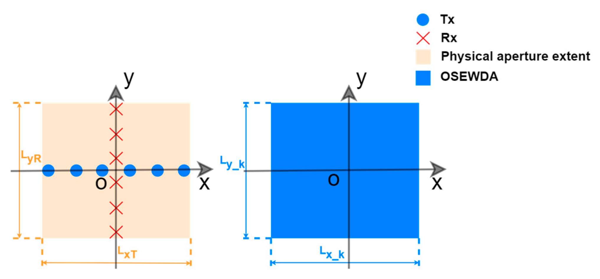
$k_{x_T}$ and $k_{y_R}$ represent the discrete wavenumber variables in azimuth and height dimensions, respectively. Similarly, based on the correspondence between wavenumber spectrum and spatial spectrum before and after ${\mathcal{F}}_{2D}^{-1}$, the output spatial extent in azimuth and height dimensions, $L_{x\_k}$ and $L_{y\_k}$ can be expressed as:

$$\left\{\begin{array}{l}{L}_{x\_k}=\left(N_T-1\right){\displaystyle \frac{2\pi }{B_{kx}}}=L_{xT}\\ L_{y\_k}=\left(N_R-1\right){\displaystyle \frac{2\pi }{B_{ky}}}=L_{yR}\end{array}\right.$$

(5)

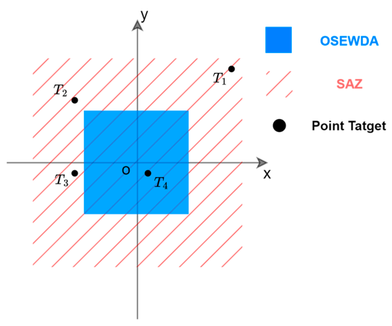
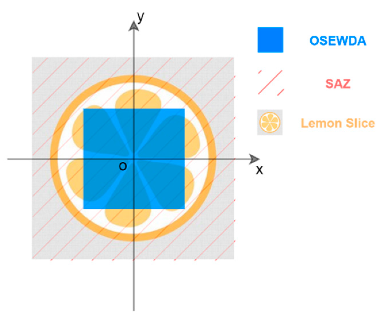
$L_{x\_k}$ and $L_{y\_k}$ are equal to the physical apertures of the 2-D cross MIMO array in azimuth and height directions, $L_{xT}$ and $L_{yR}$, respectively, as shown in Figure 2. Specifically, the Output Spatial Extent in azimuth and height dimensions of existing MIMO Wavenumber Domain Algorithms (OSEWDA) are determined by the physical aperture.

2.2. Spatial Aliasing

However, USR along both dimensions is jointly determined by the element spacing and beam angle range. The reflectivity features within USR, but outside OSEWDA, cannot be accurately reconstructed by the existing wavenumber domain algorithms. As a direct consequence, the spatial aliasing phenomenon is mathematically analyzed.

The matched filter for MIMO radar can be expressed as:

$$o\left(x,y,z\right)={\displaystyle \iiint s\left(x_{Tm},y_{Rn},k\right)}{e}^{jk{R}_{Tm}}{e}^{jk{R}_{Rn}}d{x}_{Tm}d{y}_{Rn}dk$$

(6)

The echo signal and the matched filter are complex conjugates in the spatial domain. By computing the derivative of the echo phase $\varphi \left(o\left(x,y,z\right)\right)$ with respect to $x_{Tm}$ and $y_{Rn}$, the azimuth wavenumber $k_x\left(x,y,z\right)$ and the height wavenumber $k_y\left(x,y,z\right)$ of the target located at $\left(x,y,z\right)$ can be expressed as:

$$\varphi \left(o\left(x,y,z\right)\right)=-k{R}_{Tm}-k{R}_{Rn}$$

(7)

$$\left\{\begin{array}{l}{k}_{x_T}\left(x,y,z\right)={\displaystyle \frac{\partial \varphi \left(o\left(x,y,z\right)\right)}{\partial x_{Tm}}}=-k{\displaystyle \frac{\left(x_{Tm}-x\right)}{R_{Tm}}}\\ k_{y_R}\left(x,y,z\right)={\displaystyle \frac{\partial \varphi \left(o\left(x,y,z\right)\right)}{\partial y_{Rn}}}=-k{\displaystyle \frac{\left(y_{Rn}-y\right)}{R_{Rn}}}\end{array}\right.$$

(8)

Thus, the condition for the wavenumber spectrum not to alias is:

$$\left\{\begin{array}{l}{\displaystyle \frac{B_{kx}}{2}}\ge \max \left(abs\left[k_{x_T}\left(x,y,z\right)\right]\right)\\ {\displaystyle \frac{B_{ky}}{2}}\ge \max \left(abs\left[k_{y_R}\left(x,y,z\right)\right]\right)\end{array}\right.$$

(9)

Given a fixed $z=z_0$, $k_x\left(x,y,z\right)$ and $k_y\left(x,y,z\right)$ monotonically decrease with respect to $x_{Tm}$ and $y_{Rn}$, respectively. The upper bound of the target’s wavenumber bandwidth is:

$$\left\{\begin{array}{l}\max \left(abs\left[k_{x_T}\left(x,y,z_0\right)\right]\right)={\displaystyle \frac{2\pi }{{\lambda }_{f\min }}}{\displaystyle \frac{\max \left[abs\left(x_{Tm}-x\right)\right]}{\sqrt{{\left(\max \left[abs\left(x_{Tm}-x\right)\right]\right)}^2+{\left(z_0\right)}^2}}}\\ \max \left(abs\left[k_{y_R}\left(x,y,z_0\right)\right]\right)={\displaystyle \frac{2\pi }{{\lambda }_{f\min }}}{\displaystyle \frac{\max \left[abs\left(y_{Rn}-y\right)\right]}{\sqrt{{\left(\max \left[abs\left(y_{Rn}-y\right)\right]\right)}^2+{\left(z_0\right)}^2}}}\end{array}\right.$$

(10)

Substituting Equations (4) and (10) into Equation (9), USR along azimuth and height dimensions, $L_{x\_avi}$ and $L_{y\_avi}$, can be expressed as:

$$\begin{array}{l}\left\{\begin{array}{l}{L}_{x\_avi}=2z_0\sqrt{{\displaystyle \frac{{\lambda }_{f\min }^2}{\left(4\mathrm{\Delta }{x}_T^2-{\lambda }_{f\min }^2\right)}}}-L_{x\_k},\mathrm{\Delta }{x}_T>{\displaystyle \frac{{\lambda }_{f\min }}{2}}\\ L_{x\_avi}=+\infty ,0<\mathrm{\Delta }{x}_T\le {\displaystyle \frac{{\lambda }_{f\min }}{2}}\end{array}\right.\\ \left\{\begin{array}{l}{L}_{y\_avi}=2z_0\sqrt{{\displaystyle \frac{{\lambda }_{f\min }^2}{\left(4\mathrm{\Delta }{y}_R^2-{\lambda }_{f\min }^2\right)}}}-L_{y\_k},\mathrm{\Delta }{y}_R>{\displaystyle \frac{{\lambda }_{f\min }}{2}}\\ L_{y\_avi}=+\infty ,0<\mathrm{\Delta }{y}_R\le {\displaystyle \frac{{\lambda }_{f\min }}{2}}\end{array}\right.\end{array}$$

(11)

Assuming the target is illuminated by the beam angles of all the array elements, Equation (11) represents that $L_{x\_avi}$ and $L_{y\_avi}$ are determined by the element spacing $∆x_T$ and ${∆y}_R$, the target’s range coordinate $z_0$, the minimum wavelength ${\lambda }_{f \mathrm{m}\mathrm{i}\mathrm{n}}$, and $L_{x\_k}$, $L_{y\_k}$.

When $L_{x\_avi}$ and $L_{y\_avi}$ do not exceed $L_{x\_k}$ and $L_{y\_k}$, USR is fully covered by OSEWDA. The reflectivity map within the array’s wavenumber illumination range can be fully reconstructed by the wavenumber domain algorithms.

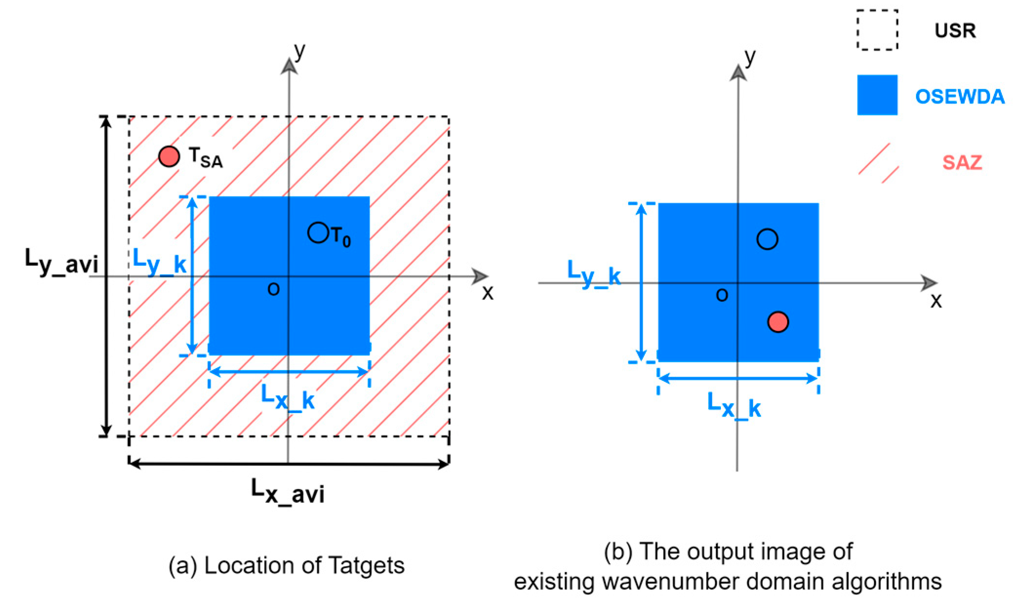
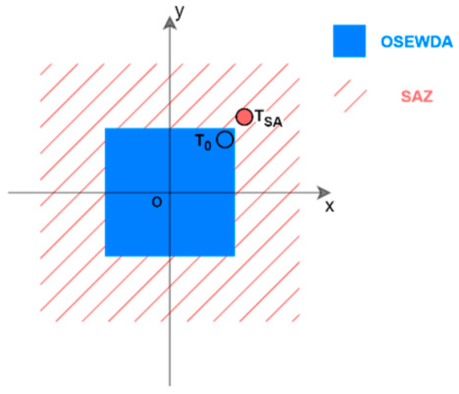
When $L_{x\_avi}$ and $L_{y\_avi}$ exceed $L_{x\_k}$ and $L_{y\_k}$, the targets within OSEWDA can also be accurately reconstructed by the algorithm: $T_0$ will be correctly mapped from the spatial location in Figure 3a to the output image in Figure 3b. For targets located outside OSEWDA but within USR, the reflectivity cannot be correctly reconstructed and will instead be aliased periodically in the output image. The reconstruction results within OSEWDA will also be affected. Since the phenomenon is analogous to spectral aliasing, the region outside OSEWDA but within USR is referred to as a “Spatial Aliasing Zone (SAZ)”. For example, in Figure 3a, $T_{SA}$ located within region SAZ has spatial coordinates that fall outside the extent of the output image. However, a response will be incorrectly reconstructed in the output image in Figure 3b.

To explain the spatial aliasing phenomenon, consider an ideal point target $T_{SA}$ located at $\left(x_{SA},y_{SA},z_{SA}\right)$ within SAZ, and derive its response in the wavenumber domain algorithm.

The echo signal of $T_{SA}$ can be expressed as:

$$s\left(x_{Tm},y_{Rn},k\right)=o\left(x_{SA},y_{SA},z_{SA}\right)e^{-jk\sqrt{{\left(x_{SA}-x_{Tm}\right)}^2+{\left(y_{SA}\right)}^2+{\left(z_{SA}\right)}^2}}{e}^{-jk\sqrt{{\left(x_{SA}\right)}^2+{\left(y_{SA}-y_{Rn}\right)}^2+{\left(z_{SA}\right)}^2}}$$

(12)

After performing 2-D FFT along azimuth and height directions, Equation (12) is transformed into:

$$\begin{array}{l}S\left(k_{x_T},k_{y_R},k\right)=o\left(x_{SA},y_{SA},z_{SA}\right)e^{-j\sqrt{k^2-k_{x_T}^2}\sqrt{{\left(y_{SA}\right)}^2+{\left(z_{SA}\right)}^2}}{e}^{-j\sqrt{k^2-k_{y_R}^2}\sqrt{{\left(x_{SA}\right)}^2+{\left(z_{SA}\right)}^2}}\times \\ e^{-j{k}_{x_T}\left(\left(x_{SA}-q{L}_{x\_k}\right)-x_{Tm}\right)}{e}^{-j{k}_{x_T}q{L}_{x\_k}}{e}^{-j{k}_{y_R}\left(\left(y_{SA}-p{L}_{y\_k}\right)-y_{Rn}\right)}{e}^{-j{k}_{y_R}p{L}_{y\_k}}\end{array}$$

(13)

$q$ and $p$ are integers, and $\left(x_0-q{L}_{x\_k}\right)ϵ\left[-L_{x\_k}/2,L_{x\_k}/2\right]$, $\left(y_0-p{L}_{y\_k}\right)ϵ\left[-L_{y\_k}/2,L_{y\_k}/2\right]$. Since $T_{SA}$ is located within the SAZ, $q$ and $p$ are not simultaneously zero. According to the Paraxial-RMA processing flow, a paraxial approximation is applied to Equation (13), resulting in:

$$\begin{array}{l}S\left(k_{x_T},k_{y_R},k\right)\approx o\left(x_{SA},y_{SA},z_{SA}\right)e^{-j2\left(\sqrt{k^2-k_{x_T}^2}+\sqrt{k^2-k_{y_R}^2}\right)z_{SA}}\times \\ e^{-j{k}_{x_T}\left(\left(x_{SA}-q{L}_{x\_k}\right)-x_{Tm}\right)}{e}^{-j{k}_{x_T}q{L}_{x\_k}}{e}^{-j{k}_{y_R}\left(\left(y_{SA}-p{L}_{y\_k}\right)-y_{Rn}\right)}{e}^{-j{k}_{y_R}p{L}_{y\_k}}\end{array}$$

(14)

After performing Stolt interpolation along $k$ direction and applying 3-D Inverse FFT (IFFT), the 3-D reconstruction result $\widehat{o}\left(x,y,z\right)$ is obtained. Assuming wavenumber spectrum in $k_{x_T}-k_{y_R}$ plane is approximated as a rectangle, the response of $T_{SA}$ can be written as:

$$\begin{array}{l}{\widehat{o}}_{\left(x_{SA},y_{SA},z_{SA}\right)}\left(x,y,z\right)\approx \delta \left(z-z_{SA}\right)\mathrm{sinc}\left({\displaystyle \frac{B_{kx}\left(x_{SA},y_{SA},z_{SA}\right)}{2}}\left[x-\left(x_{SA}-p{L}_{x\_k}\right)\right]\right)\times \\ \mathrm{sinc}\left({\displaystyle \frac{B_{ky}\left(x_{SA},y_{SA},z_{SA}\right)}{2}}\left[y-\left(y_{SA}-q{L}_{y\_k}\right)\right]\right)e^{j\left(x-x_{SA}\right)k_{xc}\left(x_{SA},y_{SA},z_{SA}\right)}{e}^{j\left(y-y_{SA}\right)k_{\mathrm{y}c}\left(x_{SA},y_{SA},z_{SA}\right)}\end{array}$$

(15)

The position where $T_{SA}$ is focused in the output image is no longer the coordinate $\left(x_{SA},y_{SA},z_{SA}\right)$, but $\left(x_{SA}-p{L}_{x\_k},y_{SA}-q{L}_{y\_k},z_{SA}\right)$.

Although the paraxial approximation in deriving point target response leads to defocusing, it can still be shown that within SAZ, the response will exhibit aliasing in the output image, which occurs with a periodicity of $L_{x\_k}$ and $L_{y\_k}$ along azimuth and height directions. Furthermore, the reconstruction quality of targets within OSEWDA will be affected.

3. Algorithm Formulation

To mitigate spatial aliasing and expand the image output spatial extent in azimuth and height dimensions, an optimization approach for the wavenumber domain algorithms is proposed, based on a sub-block imaging algorithm and spatial aliasing filter.

The preliminary reconstruction of each sub-block is achieved by the sub-block imaging algorithm. Then, the output image is matched with the corresponding spatial aliasing filter, and the complete reconstruction of the sub-block is accomplished. The aforementioned process is applied to $N_{sub}$ sub-blocks and the output image of expanded spatial extent is obtained by stitching results.

The implementation of sub-block imaging and spatial aliasing filters are presented separately below.

3.1. Sub-Block Imaging Algorithm

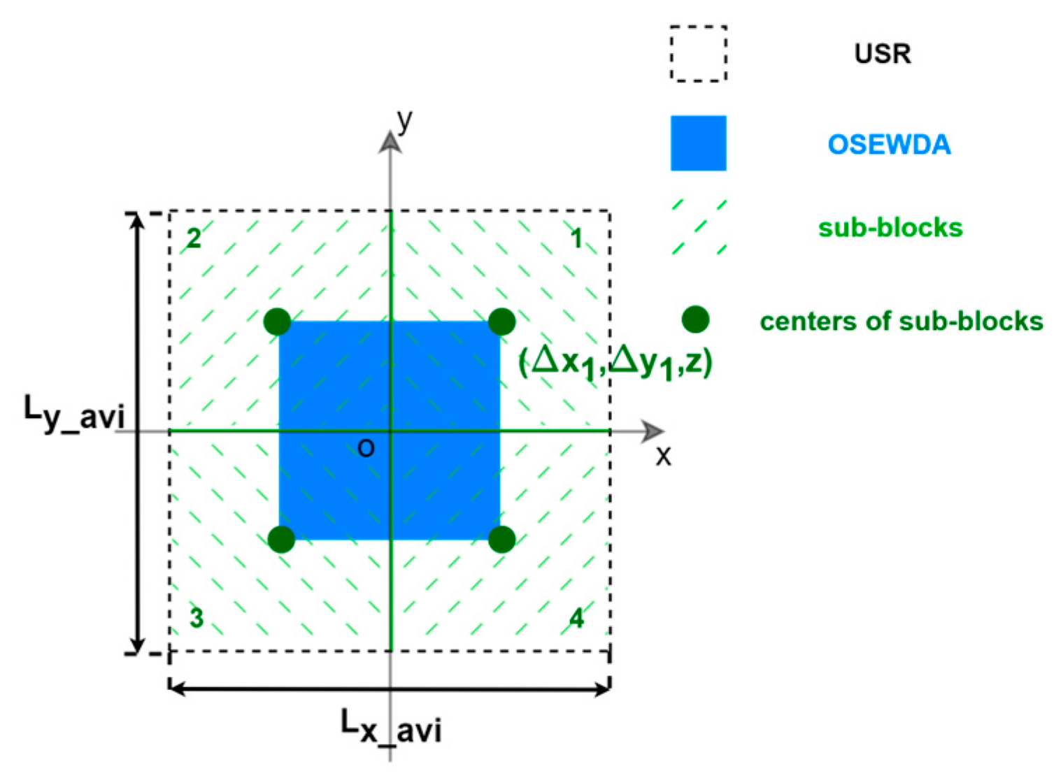
USR is divided into multiple sub-blocks, each with the same size as OSEWDA. Independent imaging is performed on each sub-block using the wavenumber domain algorithm, and the preliminary expansion of output spatial extent is achieved by stitching the sub-images, as shown in Figure 4.

The offset between each sub-block and the center of the OSEWDA requires corresponding adjustments to the wavenumber domain algorithms. Taking sub-block 1, with center coordinates $\left({∆x}_1,{∆y}_1\right)$ as shown in Figure 4 as an example, its echo expression is given by:

$$\begin{array}{l}S\left(k_{x_T},k_{y_R},k\right)={\displaystyle \iiint o\left(x_1+\mathrm{\Delta }{x}_1,y_1+\mathrm{\Delta }{y}_1,z\right)}{e}^{-j\sqrt{k^2-k_{x_T}^2}\sqrt{{\left(y_1+\mathrm{\Delta }{y}_1\right)}^2+{\left(z\right)}^2}}{e}^{-j\sqrt{k^2-k_{y_R}^2}\sqrt{{\left(x_1+\mathrm{\Delta }{x}_1\right)}^2+{\left(z\right)}^2}}\times \\ e^{-j{k}_{x_T}\left(x_1+\mathrm{\Delta }{x}_1\right)}{e}^{-j{k}_{y_R}\left(y_1+\mathrm{\Delta }{y}_1\right)}d\left(x_1+\mathrm{\Delta }{x}_1\right)d\left(y_1+\mathrm{\Delta }{y}_1\right)dz\end{array}$$

(16)

$x_1$ and $y_1$ represent the offsets relative to $\left({∆x}_1,{∆y}_1\right)$ for the target within sub-block 1, and extents being $\left(-L_{x\_k}/2,L_{x\_k}/2\right)$ and $\left(-L_{y\_k}/2,L_{y\_k}/2\right)$, respectively. The phase ${\varphi }_{Shift}$ represented by Equation (18) is matched in the 3-D wavenumber domain:

$$S_{Shifted}\left(k_{x_T},k_{y_R},k\right)=S\left(k_{x_T},k_{y_R},k\right)e^{j{\varphi }_{Shift}\left(\mathrm{\Delta }{x}_1,\mathrm{\Delta }{y}_1\right)}$$

(17)

$${\varphi }_{Shift}\left(\mathrm{\Delta }{x}_1,\mathrm{\Delta }{y}_1\right)=k_{x_T}\mathrm{\Delta }{x}_1+k_{y_R}\mathrm{\Delta }{y}_1$$

(18)

The coordinate variables coupled with $k_{x_T}$ and $k_{y_R}$ are transformed into $x_1$ and $y_1$ in Equation (17). Based on the extent of targets with sub-block 1, $xϵ\left[{∆x}_1+\left(-L_{x\_k}/2,L_{x\_k}/2\right)\right]$ and $yϵ\left[{∆y}_1+\left(-L_{y\_k}/2,L_{y\_k}/2\right)\right]$, $T_{k\_Shift}$ can be executed for wavefront correction and range focusing.

$$S_{Shifted}\left(k_{x_T},k_{y_R},z\right)=T_{k\_Shifted}\left(S_{Shifted}\left(k_{x_T},k_{y_R},k\right)\right)$$

(19)

Finally, a 2-D inverse Fourier transform is performed to complete the reconstruction of sub-block 1:

$${\widehat{o}}_{s1}\left(x,y,z\right)={\mathcal{F}}_{2D}^{-1}\left[S_{Shifted}\left(k_{x_T},k_{y_R},z\right)\right]$$

(20)

By repeating the aforementioned process, imaging results for other sub-blocks are obtained, thereby expanding the output spatial extent through stitching.

3.2. Spatial Aliasing Filter

The sub-block imaging algorithm can preliminarily expand the output spatial extent, but spatial aliasing leads to a degradation in reconstruction quality. A spatial aliasing filter based on wavenumber spectrum spatial transformation correction and rectangular window weighting is proposed.

Based on Equation (8), the wavenumber bandwidth and the wavenumber centers in azimuth and height dimensions are given by Equations (21) and (22), respectively.

$$\left\{\begin{array}{l}{B}_{kx}\left(x,y,z\right)=k{\displaystyle \frac{\left(x+L_{xT}/2\right)}{\sqrt{{\left(x+L_{xT}/2\right)}^2+{\left(y\right)}^2+{\left(z\right)}^2}}}-k{\displaystyle \frac{\left(x-L_{xT}/2\right)}{\sqrt{{\left(x-L_{xT}/2\right)}^2+{\left(y\right)}^2+{\left(z\right)}^2}}}\\ B_{ky}\left(x,y,z\right)=k{\displaystyle \frac{\left(y+L_{yR}/2\right)}{\sqrt{{\left(x\right)}^2+{\left(y+L_{yR}/2\right)}^2+{\left(z\right)}^2}}}-k{\displaystyle \frac{\left(y-L_{yR}/2\right)}{\sqrt{{\left(x\right)}^2+{\left(y-L_{yR}/2\right)}^2+{\left(z\right)}^2}}}\end{array}\right.$$

(21)

$$\left\{\begin{array}{l}{k}_{xc}\left(x,y,z\right)={\displaystyle \frac{k}{2}}\left[{\displaystyle \frac{\left(x+L_{xT}/2\right)}{\sqrt{{\left(x+L_{xT}/2\right)}^2+{\left(y\right)}^2+{\left(z\right)}^2}}}+{\displaystyle \frac{\left(x-L_{xT}/2\right)}{\sqrt{{\left(x-L_{xT}/2\right)}^2+{\left(y\right)}^2+{\left(z\right)}^2}}}\right]\\ k_{\mathrm{y}c}\left(x,y,z\right)={\displaystyle \frac{k}{2}}\left[{\displaystyle \frac{\left(y+L_{yR}/2\right)}{\sqrt{{\left(x\right)}^2+{\left(y+L_{yR}/2\right)}^2+{\left(z\right)}^2}}}+{\displaystyle \frac{\left(y-L_{yR}/2\right)}{\sqrt{{\left(x\right)}^2+{\left(y-L_{yR}/2\right)}^2+{\left(z\right)}^2}}}\right]\end{array}\right.$$

(22)

Equations (21) and (22) show that wavenumber bandwidth and the wavenumber centers vary with the spatial coordinates of the target. Matching a rectangular filter with the center of the sub-block as a reference results in energy loss. Spatially variant correction can unify wavenumber spectrum centers of the objects. By matching a rectangular filter centered at the origin, the energy of the target block can be preserved. On the contrary, the wavenumber spectrum center of targets in SAZ cannot be shifted to the origin, resulting in energy suppression.

Taking $T_0$ in the sub-block 1 with coordinates $\left(x_0,y_0,z_0\right)$ as an example, approximating the wavenumber spectrum as a rectangle, the response obtained after processing the sub-block imaging algorithm is given by:

$$\begin{array}{l}{\widehat{o}}_{s1}\left(x,y,z\right)\approx \delta \left(z-z_0\right)e^{j\left(x-x_0\right)k_{xc}\left(x_0,y_0,z_0\right)}{e}^{j\left(y-y_0\right)k_{\mathrm{y}c}\left(x_0,y_0,z_0\right)}\times \\ \mathrm{sinc}\left({\displaystyle \frac{B_{kx}\left(x_0,y_0,z_0\right)}{2}}\left(x-x_0\right)\right)\mathrm{sinc}\left({\displaystyle \frac{B_{ky}\left(x_0,y_0,z_0\right)}{2}}\left(y-y_0\right)\right)\end{array}$$

(23)

The exponential terms, $\mathrm{e}\mathrm{x}\mathrm{p}\left(j{k}_{xc}\left(x,y,z\right)x\right)$ and $\mathrm{e}\mathrm{x}\mathrm{p}\left(j{k}_{yc}\left(x,y,z\right)y\right)$, are introduced by the wavenumber center shift along $k_x$ and $k_y$, respectively [34]. Analogous to the de-skewing process in chirp signal, the exponential terms $exp\left(-j{\phi }_{xc}\right)exp\left(-j{\phi }_{yc}\right)$ are matched to the output expressed by Equation (20) in the 3-D spatial domain:

$${\widehat{o}}_{C1}\left(x,y,z\right)={\widehat{o}}_{s1}\left(x,y,z\right)e^{-j{\phi }_{xc}}{e}^{-j{\phi }_{yc}}$$

(24)

The wavenumber spectrum centers of objects in sub-block 1 are corrected to the origin. Here, ${\phi }_{xc}\left(x,y,z\right)$ and ${\phi }_{yc}\left(x,y,z\right)$ satisfy:

$$\begin{array}{l}{\left({\displaystyle \frac{\partial {\phi }_{xc}}{\partial x}}\right)}_{x=x_0}=k_{xc}\left(x_0,y_0,z_0\right)\\ {\left({\displaystyle \frac{\partial {\phi }_{yc}}{\partial y}}\right)}_{y=y_0}=k_{yc}\left(x_0,y_0,z_0\right)\end{array}$$

(25)

Substituting Equation (22) into Equation (25) yields:

$$\begin{array}{l}{\phi }_{xc}={\displaystyle \frac{k}{2}}\left[\sqrt{{\left(x+L_{xT}/2\right)}^2+{\left(y\right)}^2+{\left(z\right)}^2}+\sqrt{{\left(x-L_{xT}/2\right)}^2+{\left(y\right)}^2+{\left(z\right)}^2}\right]\\ {\phi }_{yc}={\displaystyle \frac{k}{2}}\left[\sqrt{{\left(x\right)}^2+{\left(y+L_{yR}/2\right)}^2+{\left(z\right)}^2}+\sqrt{{\left(x\right)}^2+{\left(y-L_{yR}/2\right)}^2+{\left(z\right)}^2}\right]\end{array}$$

(26)

However, applying Equation (24) to the response of target $T_{SA}$ expressed by Equation (15) in 3-D spatial domain:

$$\begin{array}{l}{\widehat{o}}_{C1}\left(x,y,z\right)=\\ {\widehat{o}}_{\left(x_{SA},y_{SA},z_{SA}\right)}\left(x,y,z\right)e^{-j{\phi }_{xc}}{e}^{-j{\phi }_{yc}}=\\ \delta \left(z-z_{SA}\right)e^{j\left[k_{xc}\left(x_{SA},y_{SA},z_{SA}\right)x-{\phi }_{xc}\left(x,y,z\right)\right]}{e}^{j\left[k_{\mathrm{y}c}\left(x_{SA},y_{SA},z_{SA}\right)y-{\phi }_{yc}\left(x,y,z\right)\right]}\times \\ \mathrm{sinc}\left({\displaystyle \frac{B_{kx}\left(x_{SA},y_{SA},z_{SA}\right)}{2}}\left[x-\left(x_{SA}-p{L}_{x\_k}\right)\right]\right)e^{-j{k}_{xc}\left(x_{SA},y_{SA},z_{SA}\right)x_{SA}}\times \\ \mathrm{sinc}\left({\displaystyle \frac{B_{ky}\left(x_{SA},y_{SA},z_{SA}\right)}{2}}\left[y-\left(y_{SA}-q{L}_{y\_k}\right)\right]\right)e^{-j{k}_{\mathrm{y}c}\left(x_{SA},y_{SA},z_{SA}\right)y_{SA}}\end{array}$$

(27)

The derivatives of ${\phi }_{xc}$ and ${\phi }_{yc}$ at $\left(x_{SA}-p{L}_{x\_k},y_{SA}-q{L}_{y\_k},z_{SA}\right)$ do not equal the origin, since $p$ and $q$ are not simultaneously zero. Following the spatially variant correction described in Equation (24), the wavenumber center of $T_{SA}$ is adjusted to:

$$\begin{array}{l}{k}_{xc\_Shifted}\left(x_{SA},y_{SA},z_{SA}\right)=k_{xc}\left(x_{SA},y_{SA},z_{SA}\right)-k_{xc}\left(\left(x_{SA}-p{L}_{x\_k}\right),\left(y_{SA}-q{L}_{y\_k}\right),z_{SA}\right)\\ k_{\mathrm{y}c\_Shifted}\left(x_{SA},y_{SA},z_{SA}\right)=k_{yc}\left(x_{SA},y_{SA},z_{SA}\right)-k_{yc}\left(\left(x_{SA}-p{L}_{x\_k}\right),\left(y_{SA}-q{L}_{y\_k}\right),z_{SA}\right)\end{array}$$

(28)

After spatially variant correction, the image $o_{c1}\left(x,y,z\right)$ is subjected to a 2-D Fourier transform along azimuth and height directions, and the rectangular filter $w\left(k_{x_T},k_{y_R},z\right)$ is applied to suppress aliasing in 2-D wavenumber domain and 1-D spatial domain:

$$O_{filtered}\left(k_{x_T},k_{y_R},z\right)={\mathcal{F}}_{2D}\left({\widehat{o}}_{C1}\left(x,y,z\right)\right)w\left(k_{x_T},k_{y_R},z\right)$$

(29)

$$w\left(k_{x_T},k_{y_R},z\right)=\mathrm{rect}\left({\displaystyle \frac{k_{x_T}}{\max \left(B_{kx}\left(x_0,y_0,z\right)\right)/2}}\right)\mathrm{rect}\left({\displaystyle \frac{k_{y_R}}{\max \left(B_{ky}\left(x_0,y_0,z\right)\right)/2}}\right)$$

(30)

After Equation (29), the energy of $T_0$ in the sub-block 1 is preserved, while the energy of $T_{\mathrm{S}\mathrm{A}}$ in SAZ is attenuated. The amount of attenuation varies with the spatial coordinates. The image of sub-block 1 after matching the spatial aliasing filter is:

$${\widehat{o}}_{sf\_1}\left(x,y,z\right)={\mathcal{F}}_{2D}^{-1}\left(O_{filtered}\left(k_{x_T},k_{y_R},z\right)\right)$$

(31)

By concatenating the images of different sub-blocks, the complete expansion of output spatial extent is achieved:

$${\widehat{o}}_{combined}\left(x,y,z\right)=\mathrm{concat}\left({\widehat{o}}_{sf\_1},{\widehat{o}}_{sf\_2},\cdots {\widehat{o}}_{sf\_N_{sub}}\right)$$

(32)

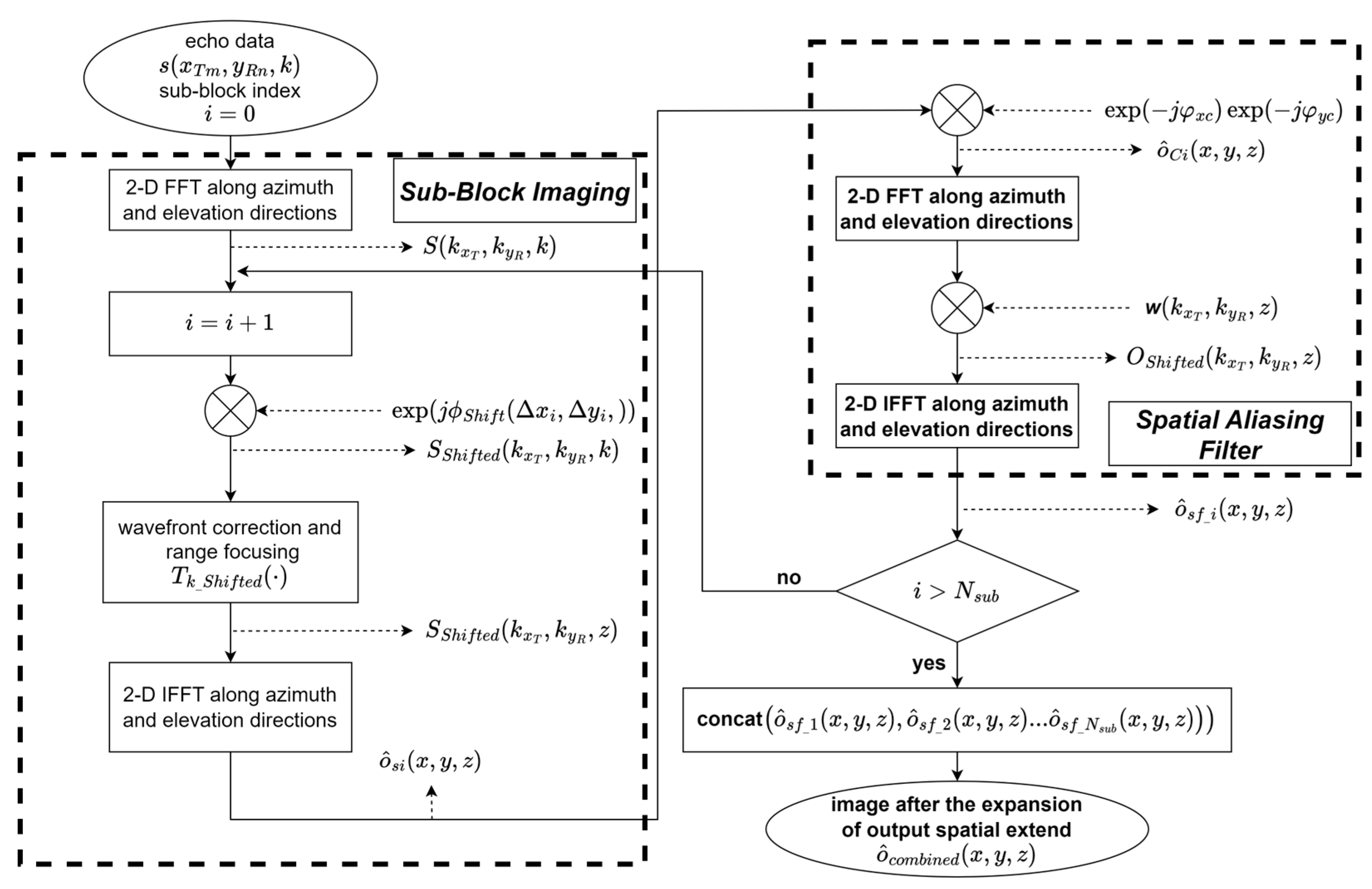
Based on the preceding description, implementation of the expansion algorithm is shown in Figure 5. The echo data $s\left(x_{Tm},y_{Rn},k\right)$ is first utilized to perform sub-block imaging algorithm, resulting in preliminary reconstruction of sub-block 1 ${\widehat{o}}_{s1}\left(x,y,z\right)$. Then, the spatial aliasing filter is applied to ${\widehat{o}}_{s1}\left(x,y,z\right)$, yielding the final reconstruction of subblock 1 ${\widehat{o}}_{sf\_1}\left(x,y,z\right)$. The process is repeated to obtain ${\widehat{o}}_{sf\_2}\left(x,y,z\right)$ to ${\widehat{o}}_{sf\_N_{sub}}\left(x,y,z\right)$ for all other sub-blocks. Finally, the output images are stitched to obtain the expanded image ${\widehat{o}}_{combined}\left(x,y,z\right)$.

It should be noted that after spatially variant correction, the wavenumber spectra of target sub-block and SAZ may overlap. The condition for the proposed filter to completely eliminate the energy in SAZ is:

$$\begin{array}{l}{\displaystyle \frac{B_{kx}\left(x_0,y_0,z_0\right)}{2}}<\mathrm{abs}\left(k_{xc\_Shifted}\left(x_{SA},y_{SA},z_{SA}\right)\right)-{\displaystyle \frac{B_{kx}\left(x_{SA},y_{SA},z_{SA}\right)}{2}}\\ or\\ {\displaystyle \frac{B_{ky}\left(x_0,y_0,z_0\right)}{2}}<\mathrm{abs}\left(k_{\mathrm{y}c\_Shifted}\left(x_{SA},y_{SA},z_{SA}\right)\right)-{\displaystyle \frac{B_{ky}\left(x_{SA},y_{SA},z_{SA}\right)}{2}}\end{array}$$

(33)

3.3. Computation Complexity

To evaluate efficiency of the algorithms, Floating-Point Operation (FLOP) are used to measure the computational complexity [35]. Prior to multi sub-blocks reconstruction, the FLOPs required for the reconstruction of OSEWDA using BPA, Paraxial-RMA, and Cross-RMA are denoted as $C_{BPA}$, $C_{Paraxial-RMA}$ and $C_{Cross-RMA}$, respectively, as specified in Appendix A. $N_{ker}$ denotes the kernel length of 1-D interpolation. $N_K$ represents the number of frequencies. $N_x,N_{y,}$ and $N_z$ represent the output image sizes along $x,y$, and $z$ directions, respectively.

In the imaging for more than one sub-block, the FLOPs generated by steps 2 to 4 of BPA will increase by a factor of $N_{sub}$, resulting in a total computational cost of:

$$C_{N_{sub}-BPA}=5N_T{N}_R{N}_K{\log }_2{N}_K+N_{sub}\left[\left(4N_{ker}+6\right)N_T{N}_R{N}_x{N}_y{N}_z\right]$$

(34)

According to Figure 5, some additional operations are incorporated into the image reconstruction of a specific sub-block for Paraxial-RMA and Cross-RMA: 1. In the sub-block imaging algorithm, a phase factor matching step, as shown in Equation (17), is added, with FLOPs of $6N_T{N}_R{N}_K$; 2. The spatial aliasing filter involves two complex multiplication operations in Equations (24) and (29), with FLOPs of $12N_T{N}_R{N}_z$; 3. 2-D FFT and IFFT for spatial-to-wavenumber domain conversion is added, with FLOPs of $10N_T{N}_R{N}_z{log}_2\left(N_T{N}_R\right)$. The sum FLOPs of the additional operations is denoted as:

$$C_{RMA-add}=6N_T{N}_R{N}_K+12N_T{N}_R{N}_z+10N_T{N}_R{N}_z{\log }_2\left(N_T{N}_R\right)$$

(35)

In the imaging for $N_{sub}$ sub-blocks, the total FLOPs of the two modified RMAs can be expressed as:

$$C_{Modified-RMA}=N_{sub}\left(C_{RMA}+C_{RMA-add}\right)$$

(36)

$C_{RMA}$ can be either $C_{Paraxial-RMA}$ or $C_{Cross-RMA}$.

Based on the analysis of FLOPs for different algorithm, a comparison is provided in

Table 1. Computational complexity comparison of different algorithms.

Algorithm	FLOPs	Approximate Complexity
BPA	$N_T{N}_R\left(5N_K{\mathrm{l}\mathrm{o}\mathrm{g}}_2{N}_K+\left(4N_{ker}+6\right)N_x{N}_y{N}_z\right)$	$O\left(N^5\right)$
Paraxial-RMA	$5N_T{N}_R\left(N_K{\mathrm{l}\mathrm{o}\mathrm{g}}_2\left(N_T{N}_R\right)+N_z{\mathrm{l}\mathrm{o}\mathrm{g}}_2\left(N_T{N}_R{N}_z\right)\right)+2N_T{N}_R{N}_z\left(2N_{ker}-1\right)$	$O\left(N^3{log}_2\left(N\right)\right)$
Cross-RMA	$\begin{array}{c}5N_T{N}_R{N}_K{\mathrm{l}\mathrm{o}\mathrm{g}}_2\left(N_T{N}_R\right)+2N_T{N}_R{N}_{\mathrm{z}}\left(4N_{ker}+3\right)+\\ N_T{N}_R{N}_z^2\left(14+5{\mathrm{l}\mathrm{o}\mathrm{g}}_2\left(N_T{N}_R\right)\right)\end{array}$	$O\left(N^4{log}_2\left(N\right)\right)$
$N_{Sub}$-BPA	$N_T{N}_R\left(5N_K{\mathrm{l}\mathrm{o}\mathrm{g}}_2{N}_k+\left(4N_{ker}+6\right)N_{sub}{N}_x{N}_y{N}_z\right)$	$O\left(N_{Sub}{N}^5\right)$
Modified Paraxial-RMA	$N_{sub}\left[\begin{array}{c}5N_T{N}_R\left(N_K{\mathrm{l}\mathrm{o}\mathrm{g}}_2\left(N_T{N}_R\right)+N_z{\mathrm{l}\mathrm{o}\mathrm{g}}_2\left(N_T{N}_R{N}_z\right)\right)+\\ 2N_T{N}_R{N}_z\left(2N_{ker}+5\right)+6N_T{N}_R{N}_K+\\ 10N_T{N}_R{N}_z{\mathrm{l}\mathrm{o}\mathrm{g}}_2\left(N_T{N}_R\right)\end{array}\right]$	$O\left({N_{Sub}N}^3{log}_2\left(N\right)\right)$
Modified Cross-RMA	$N_{sub}\left[\begin{array}{c}5N_T{N}_R{N}_K{\mathrm{l}\mathrm{o}\mathrm{g}}_2\left(N_T{N}_R\right)+2N_T{N}_R{N}_{\mathrm{z}}(4N_{ker}+9)+\\ N_T{N}_R{N}_z^2\left(14+5{\mathrm{l}\mathrm{o}\mathrm{g}}_2\left(N_T{N}_R\right)\right)+6N_T{N}_R{N}_K+\\ +10N_T{N}_R{N}_z{\mathrm{l}\mathrm{o}\mathrm{g}}_2\left(N_T{N}_R\right)\end{array}\right]$	$O\left({N_{Sub}N}^4{log}_2\left(N\right)\right)$

. Considering that the discrete sampling quantities $N_T$, $N_R$, $N_K$, $N_x$, $N_y,$ and $N_z$ are of the same order of magnitude as $N$, the algorithm’s approximate complexity is represented in the third column of Table 1.

After the output spatial extent is expanded, the computational complexity of BPA and wavenumber domain algorithms increases by approximately a factor of $N_{Sub}$. However, the modified wavenumber algorithms remain significantly lower than that of $N_{Sub}$-BPA.

4. Experiments

The aliasing suppression and output spatial extent expansion capability of the modified wavenumber domain algorithms are demonstrated by simulations in this section. The hardware platform for simulations is equipped with a 13th Gen Intel(R) Core(TM) i5-13500 processor, with a clock speed of 2.50 GHz and 32 GB of RAM.

The Stepped Frequency Continuous Wave (SFCW) is the signal model used in the simulations. The array configuration follows the 2-D cross MIMO array shown in Figure 1. The parameter settings are provided in

Table 2. Parameter setup for the experiments.

Parameter Description	Parameter Value
Center frequency	140 GHz
Bandwidth	20 GHz
Number of stepped frequencies	256
Number of transmitters	100
Transmitting interval	0.00153 m
Number of receivers	100
Receiving interval	0.00153 m

.

4.1. Simulation of Sub-Block Imaging Algorithm

In Simulation A, the imaging scene is set up with a lemon slice-shaped target, which is of the same size as OSEWDA. The center of lemon slice is $\left(0.0755,0.0755,0.224\right) \mathrm{m}$, as shown in Figure 6. The orange pixels represent ideal point targets with a reflectivity of 1, and the other locations have a reflectivity of 0.

The echo data from Simulation A is processed using Cross-RMA, Paraxial-RMA, and BPA, along with the corresponding sub-block imaging algorithms. The output spatial extents of the sub-block imaging algorithms have the centers aligned with the lemon slice. The first row of Figure 7 shows that the targets within OSEWDA are correctly reconstructed using the algorithms without center shift of output spatial extent. However, accurate reconstruction fails to occur for targets outside of OSEWDA, thereby inducing spatial aliasing in the output images of Paraxial-RMA and Cross-RMA. After applying the sub-block imaging algorithms, the center of the output spatial extent is shifted from $\left(0, 0, 0.224\right) \mathrm{m}$ to $\left(0.0755, 0.0755, 0.224\right) \mathrm{m}$. The lemon slice is fully covered by the modified output spatial extent, resulting in a complete reconstruction, as shown in the second row of Figure 7. To evaluate reconstruction accuracy of the wavenumber domain algorithms after center shift, the correlation coefficient $r$ between the output image and the BPA output image [31] is computed with:

$$r={\displaystyle {\sum }_{i,j,k}\left|\frac{{\widehat{o}}_{RMA}(x_i,y_j,z_k)}{\sqrt{{\displaystyle {\sum }_{i,j,k}{\left|{\widehat{o}}_{RMA}(x_i,y_j,z_k)\right|}^2}}}\cdot \frac{{\widehat{o}}_{BPA}(x_i,y_j,z_k)}{\sqrt{{\displaystyle {\sum }_{i,j,k}{\left|{\widehat{o}}_{BPA}(x_i,y_j,z_k)\right|}^2}}}\right|}$$

(37)

In Simulation A, ${\widehat{o}}_{RMA}$ can be either the output image of Paraxial-RMA or Cross-RMA after center shift. ${\widehat{o}}_{BPA}$ represents the output image of BPA after center shift. The $r$ corresponding to Paraxial-RMA and Cross-RMA are 0.0926 and 0.9949, respectively.

After the center shift, the shape of the lemon slice-shaped target is roughly reconstructed in the output image of Paraxial-RMA. The errors introduced by paraxial approximation result in poor consistency with the output image of BPA. With higher reconstruction accuracy, the consistency between the output images of Cross-RMA and BPA is very strong after center shift.

4.2. Simulation of Spatial Aliasing Filter

In Simulation B-I, point targets $T_0$ and $T_{SA}$ are set up inside and outside the OSEWDA, respectively, as shown in Figure 8. The coordinates of $T_0$ and $T_{SA}$ are $\left(0.0694, 0.0694, 0.224\right)\mathrm{m}$ and $\left(0.0801, 0.0801, 0.224\right)\mathrm{m}$, with a reflectivity of 1 for both.

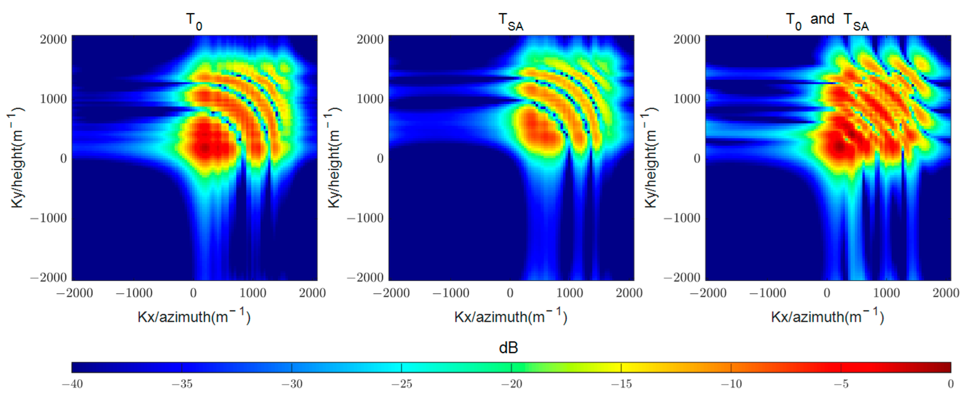
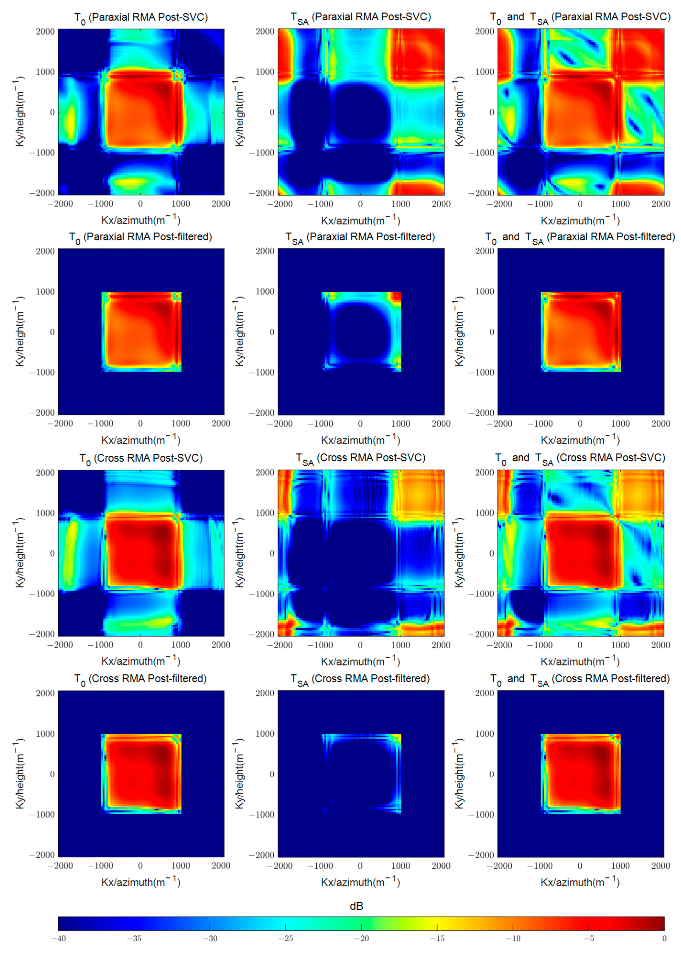
The echo data from Simulation B-I is processed using Paraxial-RMA and Cross-RMA, along with the corresponding improved algorithms that incorporate spatial aliasing filter. Simulation B-I generates three echo signals, with the scene setups as follows: containing only $T_0$, containing only $T_{SA}$, and containing both $T_0$ and $T_{SA}$.

Figure 9 shows that the wavenumber spectra of $T_0$ and $T_{SA}$ overlap significantly. Direct matching of rectangular window in the wavenumber domain cannot achieve energy separation.

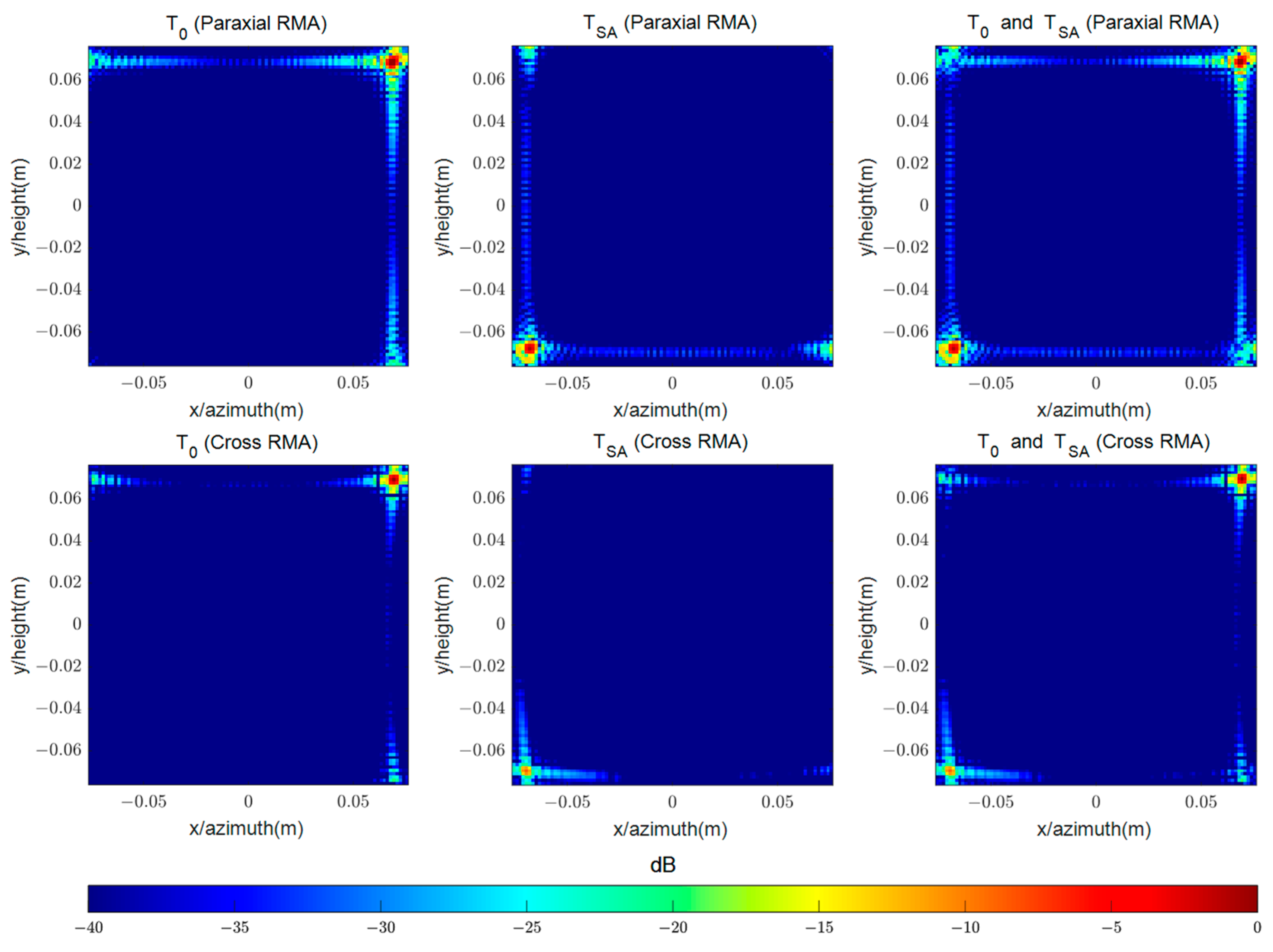
Figure 10 shows that the output images of Paraxial-RMA and Cross-RMA contain both the correct reconstruction of $T_0$ and the aliased response of $T_{SA}$.

Figure 11 shows the wavenumber spectra after matching proposed spatial aliasing filter. Spatial variation correction separates the wavenumber spectra of $T_0$ and $T_{SA}$.

Table 3. Spectral energy suppression in wavenumber domain by the proposed spatial aliasing filter.

	Target	${\mathit{T}}_0$	${\mathit{T}}_{\mathit{S}\mathit{A}}$
Algorithm
Paraxial-RMA		0.27652 dB	14.5541 dB
Cross-RMA		0.32588 dB	17.0123 dB

indicates that after matching the rectangular window, the wavenumber spectral energy of $T_0$ is relatively well preserved, while the energy of $T_{SA}$ is effectively suppressed. The aliasing suppression capability of the proposed filter is first demonstrated by the attenuation of wavenumber spectral energy:

$$\mathrm{Power}\mathrm{Attenuation}=10{\log }_{10}\left({\displaystyle \frac{{\displaystyle \sum _{k_{x_T}}{\displaystyle \sum _{k_{y_R}}{\displaystyle \sum _{z\text{'}}{\left(O_{filtered}\left(k_{x_T},k_{y_R},z\text{'}\right)\right)}^2}}}}{{\displaystyle \sum _{k_{x_T}}{\displaystyle \sum _{k_{y_R}}{\displaystyle \sum _{z\text{'}}{\left({\mathcal{F}}_{2D}\left[o_C\left(x\text{'},y\text{'},z\text{'}\right)\right]\right)}^2}}}}}\right)$$

(38)

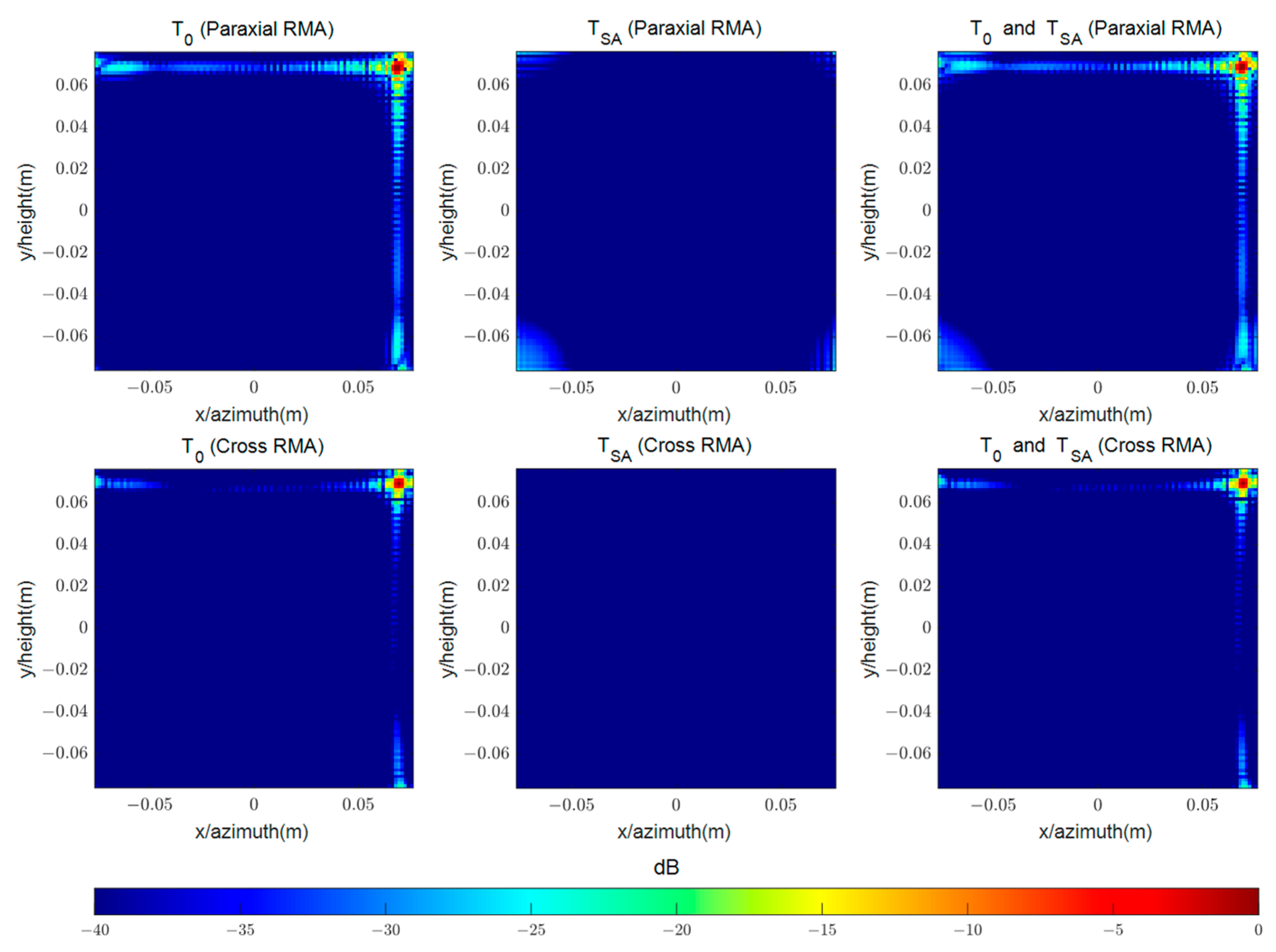
Figure 12 shows the output images after matching spatial aliasing filter. The aliasing suppression capability is further demonstrated by the attenuation of peak amplitude:

$$\mathrm{Attenuation}=20{\log }_{10}\left({\displaystyle \frac{\underset{x\text{'},y\text{'},z\text{'}}{\max }\left(\mathrm{abs}\left[o_{filtered}\left(x\text{'},y\text{'},z\text{'}\right)\right]\right)}{\underset{x\text{'},y\text{'},z\text{'}}{\max }\left(\mathrm{abs}\left[o_C\left(x\text{'},y\text{'},z\text{'}\right)\right]\right)}}\right)$$

(39)

Table 4. Peak amplitude suppression in the output images by the proposed spatial aliasing filter.

	Target	${\mathit{T}}_0$	${\mathit{T}}_{\mathit{S}\mathit{A}}$
Algorithm
Paraxial-RMA		0.40124 dB	29.2975 dB
Cross-RMA		0.28343 dB	29.0126 dB

indicates that the peak amplitude level of $T_0$’s output image exhibits almost no attenuation, while level of $T_{\mathrm{S}\mathrm{A}}$ is effectively suppressed.

Simulation B-I demonstrates the suppression of spatial aliasing by the proposed filter. To assess the performance at different spatial locations, Simulation B-II keeps the other parameters from Simulation B-I unchanged, with only the azimuth and height coordinates of the point target being modified.

Figure 13 and Figure 14 illustrate the suppression levels of the wavenumber spectral energy and the image peak amplitude achieved by the filter for targets at different positions, respectively. Table 5 and Table 6 present the statistical results of Figure 13 and Figure 14, respectively.

Table 5. Statistical result of wavenumber spectrum energy suppression by the proposed spatial aliasing filter.

	Locations of Target	Sub-Block to Be Imaged			SAZ
Algorithm
		Min	Avg	Max	Min	Avg	Max
Paraxial-RMA		0.061 dB	1.015 dB	4.052 dB	7.744 dB	19.117 dB	26.781 dB
Cross-RMA		0.009 dB	0.462 dB	2.018 dB	9.422 dB	23.364 dB	29.609 dB

Table 5. Statistical result of wavenumber spectrum energy suppression by the proposed spatial aliasing filter.

	Locations of Target	Sub-Block to Be Imaged			SAZ
Algorithm
		Min	Avg	Max	Min	Avg	Max
Paraxial-RMA		0.061 dB	1.015 dB	4.052 dB	7.744 dB	19.117 dB	26.781 dB
Cross-RMA		0.009 dB	0.462 dB	2.018 dB	9.422 dB	23.364 dB	29.609 dB

Table 6. Statistical Result of Peak Amplitude Suppression by the Proposed Spatial Aliasing Filter.

	Locations of Target	Sub-Block to Be Imaged			SAZ
Algorithm
		Min	Avg	Max	Min	Avg	Max
Paraxial-RMA		0.033 dB	1.083 dB	4.606 dB	11.731 dB	24.894 dB	35.038 dB
Cross-RMA		0.009 dB	0.622 dB	3.126 dB	13.722 dB	31.134 dB	53.143 dB

Table 6. Statistical Result of Peak Amplitude Suppression by the Proposed Spatial Aliasing Filter.

	Locations of Target	Sub-Block to Be Imaged			SAZ
Algorithm
		Min	Avg	Max	Min	Avg	Max
Paraxial-RMA		0.033 dB	1.083 dB	4.606 dB	11.731 dB	24.894 dB	35.038 dB
Cross-RMA		0.009 dB	0.622 dB	3.126 dB	13.722 dB	31.134 dB	53.143 dB

In the sub-block to be imaged, spatial aliasing filter achieves an average wavenumber spectrum energy suppression level of 1.015 dB and 0.462 dB for Paraxial-RMA and Cross-RMA, respectively. The corresponding attenuation of peak amplitude is 1.083 dB and 0.622 dB.

In SAZ, spatial aliasing filter achieves an average wavenumber spectrum energy suppression level of 19.117 dB and 23.364 dB for the Paraxial-RMA and Cross-RMA, respectively. The corresponding attenuation of peak amplitude is 24.894 dB and 31.134 dB.

Simulation B-II demonstrates that the proposed filter exhibits repeatability in both the sub-block to be imaged and SAZ. In other words, the responses of the former and the latter are preserved and suppressed, respectively. In addition, the filter demonstrates better performance in Cross-RMA, which has better reconstruction accuracy.

4.3. Simulation of Output Spatial Extent Expansion

In simulation C-I, point targets $T_1$ to $T_4$ are located at different quadrants, and the coordinates are $\left(0.138, 0.138, 0.224\right) \mathrm{m}$, $\left(-0.0923, 0.0923, 0.224\right) \mathrm{m}$, $\left(-0.0923, -0.0160, 0.224\right) \mathrm{m}$, and $\left(0.0160, -0.0160, 0.224\right) \mathrm{m}$, as shown in Figure 15. The reflectivity of the targets is set to 1.

The echo of Simulation C-I is processed using Paraxial-RMA, Cross-RMA, and the improved algorithms, resulting in the output images in Figure 16. In the improved Paraxial-RMA and Cross-RMA, the extended extent is divided into four sub-blocks, each located in a different quadrant. The output images in the first and second rows, which are normalized with respect to the maximum values of the output images from Paraxial-RMA and Cross-RMA, are shown in Figure 16.

In the first column of Figure 16, only target $T_4$ within OSEWDA is correctly reconstructed, while the responses of other targets are aliased in the output image. Employing the proposed sub-block imaging algorithm expands the output spatial extent, allowing targets $T_1$ to $T_4$ to be reconstructed. However, aliasing remains in the images, as shown in the second column. In the third column, the proposed filter is applied to each sub-block of the images in the second column, resulting in the suppression of aliased energy.

The output image of BPA is shown in the first column of Figure 17. The correlation coefficient $r$ corresponding to Paraxial-RMA and Cross-RMA are 0.2202 and 0.9746, respectively. To better illustrate correlation coefficient, the difference between output image of BPA and the improved Paraxial-RMA is shown in the second column of Figure 17. The third column presents the difference between output image of BPA and the improved Cross-RMA.

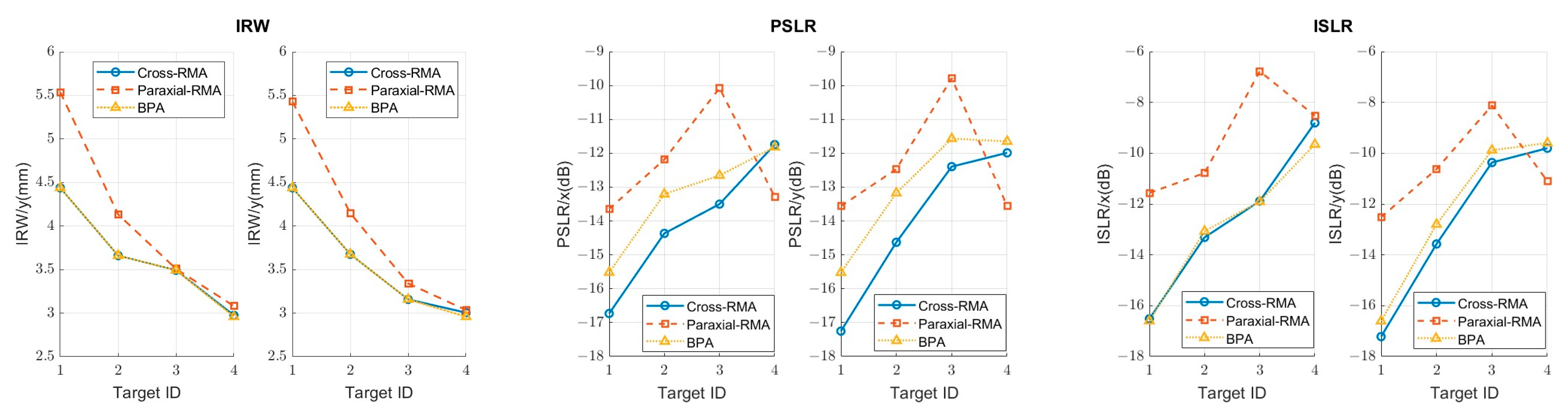
The Impulse Response Width (IRW), Peak Sidelobe Ratio (PSLR), and Integrated Sidelobe Ratio (ISLR) of targets $T_1$ to $T_4$ in the third column of Figure 16, as well as the output image of BPA, are provided in Figure 18.

The analysis of Figure 18 reveals differences in IRW, PSLR, and ISLR between BPA and Paraxial-RMA, as well as the differences between BPA and Cross-RMA, as shown in Table 7. The differences are formally quantified through:

$$Dif\left(Parameter\right)={\displaystyle \frac{{\displaystyle \sum _{i=1}^{4}abs\left[BP{A}_{Parameter}\left(i\right)-RM{A}_{Parameter}\left(i\right)\right]}}{4}}$$

(40)

$Parameter$ can be IRW, PSLR, or ISLR. $i$ represents the ID of targets.

Table 7. The Metrics Difference between BPA and Paraxial-RMA, as well as the Metrics Difference between BPA and Cross-RMA.

Algorithm	Paraxial-RMA			Cross-RMA
Parameter	IRW	PSLR	ISLR	IRW	PSLR	ISLR
Difference with BPA/x	0.427 mm	1.734 dB	3.396 dB	0.00381 mm	0.823 dB	0.299 dB
Difference with BPA/y	0.507 mm	1.590 dB	2.379 dB	0.0915 mm	1.087 dB	0.519 dB

Table 7. The Metrics Difference between BPA and Paraxial-RMA, as well as the Metrics Difference between BPA and Cross-RMA.

Algorithm	Paraxial-RMA			Cross-RMA
Parameter	IRW	PSLR	ISLR	IRW	PSLR	ISLR
Difference with BPA/x	0.427 mm	1.734 dB	3.396 dB	0.00381 mm	0.823 dB	0.299 dB
Difference with BPA/y	0.507 mm	1.590 dB	2.379 dB	0.0915 mm	1.087 dB	0.519 dB

Table 7 shows that within a certain difference, the RMA algorithms exhibit qualities close to BPA in point target response. Moreover, Cross-RMA exhibits smaller parameter differences compared to Paraxial-RMA.

In Simulation C-II, a lemon slice with dimensions of 0.302 m × 0.302 m is set, with its center at $\left(0, 0, 0.224\right) \mathrm{m}$, as shown in Figure 19. The orange pixels represent ideal point targets with a reflectivity of 1, and the other locations have a reflectivity of 0.

The echo data from Simulation C-II is processed using the same procedure as Simulation C-I, and the output image is shown in Figure 20. The first column shows that both Cross-RMA and Paraxial-RMA fail to reconstruct planar targets larger than the OSEWDA. Employing the proposed sub-block imaging algorithm expands the output spatial extent, but aliasing remains in the images, as shown in the second column. Finally, the large-sized planar target is reconstructed by matching proposed spatial aliasing filter to the output images of each sub-block, as shown in the last column.

The output image of BPA is shown in the first column of Figure 21. The correlation coefficient $r$ corresponding to Paraxial-RMA and Cross-RMA are 0.3533 and 0.9795, respectively. The difference between output image of BPA and the improved Paraxial-RMA is shown in the second column of Figure 21. The third column presents the difference between output image of BPA and the improved Cross-RMA.

Figure 20 and Figure 21 demonstrate that the proposed extended algorithm maintains reconstruction performance in planar target imaging.

The computation time of different algorithms are presented in

Table 8. Time consumption of different algorithm.

Algorithm	Paraxial-RMA		Cross-RMA		BPA
	1 Block	4 Blocks	1 Block	4 Blocks	1 Block	4 Blocks
Time Consumption/s	0.222	1.329	12.239	50.670	1228.122	4719.616

. A cubic kernel with a length of 4 is used for the interpolation operations.

Table 8 shows that the time consumption of BPA for imaging one sub-block is 5532 and 100 times that of Paraxial-RMA and Cross-RMA, respectively. After the sub-blocks were expanded to 4, the time consumption of algorithms increased by approximately 3 times. The RMA algorithms maintain the advantage of low time consumption compared to BPA.

In Simulation C-III, a handgun model with dimensions of 0.302 m × 0.302 m is set, with its center at $\left(0, 0, 0.224\right) \mathrm{m}$, as shown in Figure 22. The orange pixels represent ideal point targets with a reflectivity of 1, and the other locations have a reflectivity of 0.

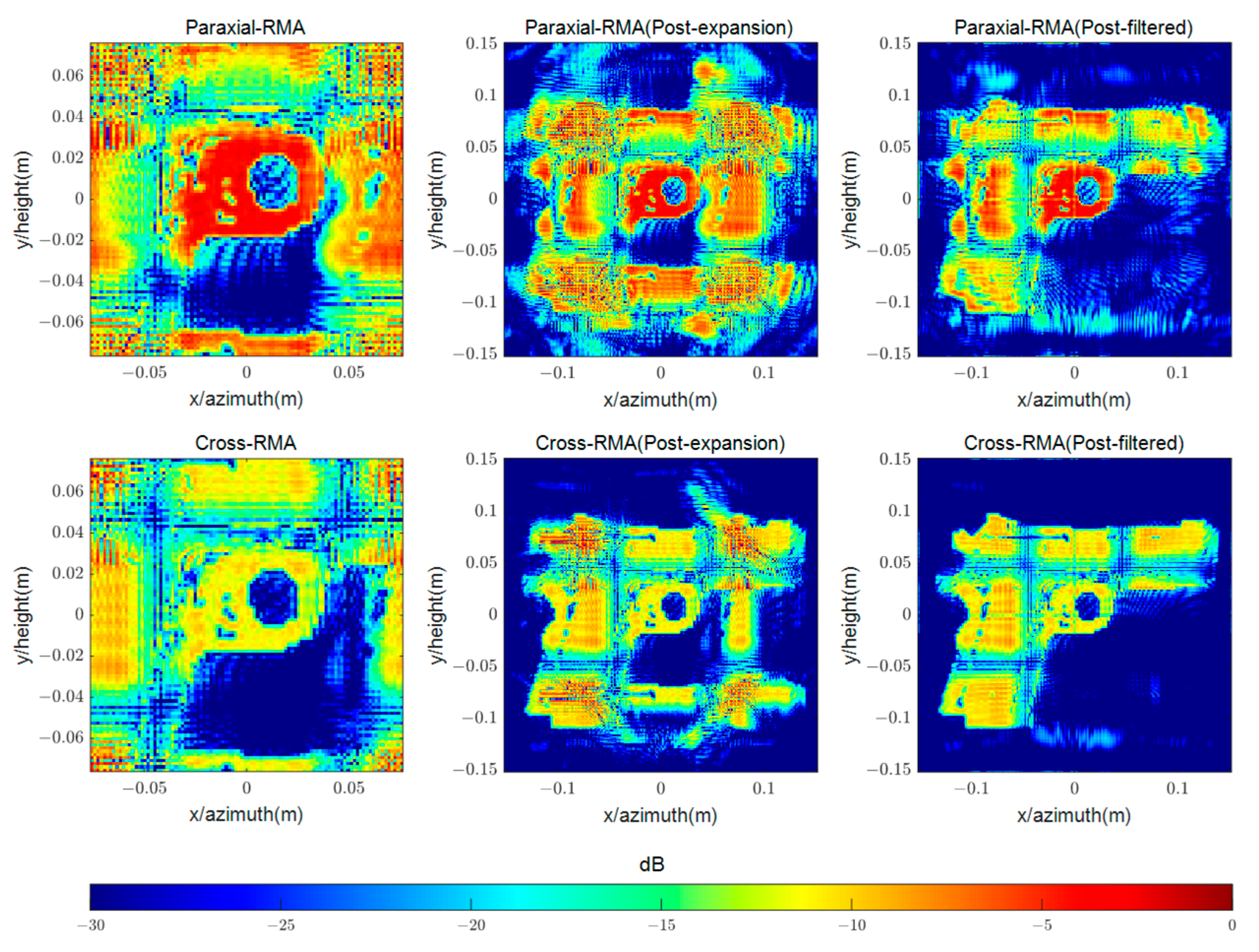
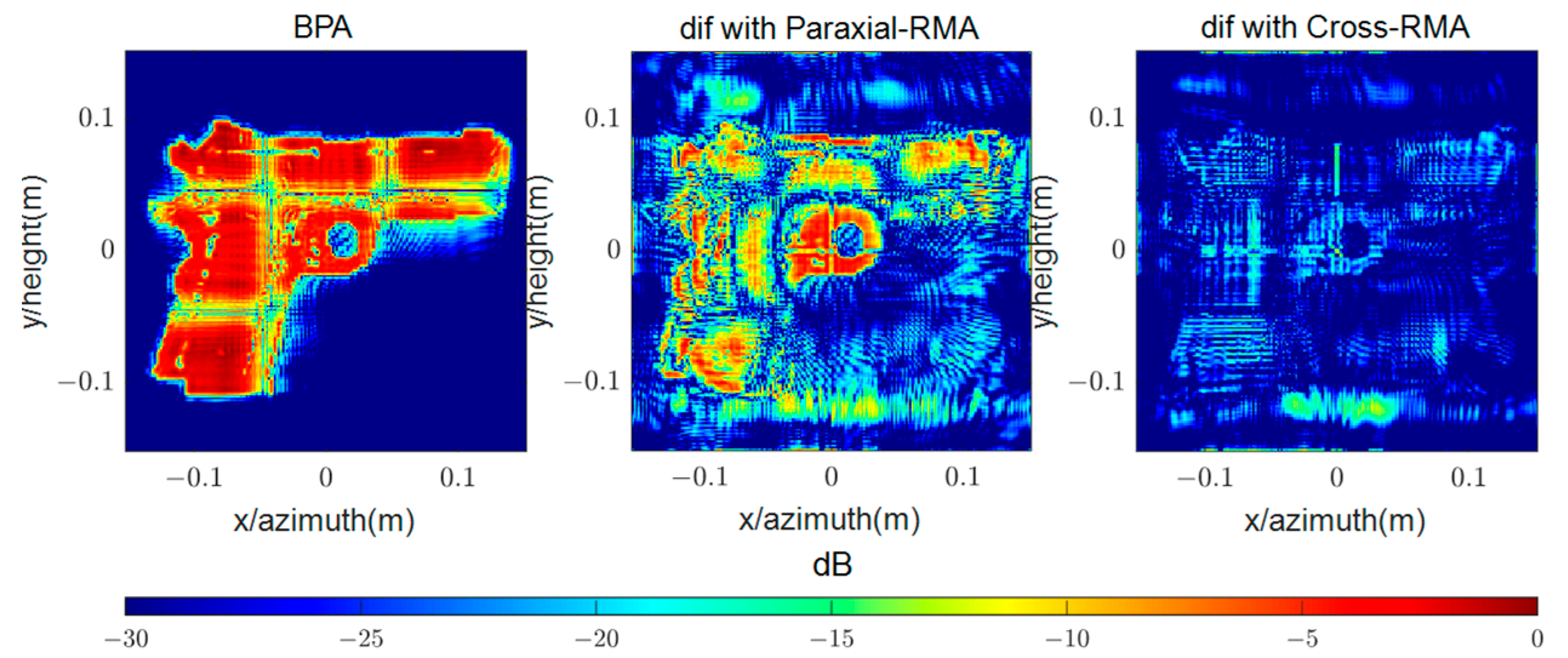
The echo data from Simulation C-III is processed using the same procedure as Simulation C-I, and the output image is shown in Figure 23 and Figure 24.

The correlation coefficient $r$ corresponding to Paraxial-RMA and Cross-RMA are 0.2518 and 0.9843, respectively. Experiments II and III indicate that the expansion capability of the proposed algorithm can be reproduced on planar targets of different shapes.

5. Conclusions

The theoretical derivation in this paper addresses the inconsistency between the output spatial extent of existing wavenumber domain imaging algorithms and the USR of MIMO array. Targets within SAZ cannot be correctly reconstructed, and aliasing is introduced into the output image.

An optimization for expanding output spatial extent in the wavenumber domain algorithms has been proposed. The proposed optimization consists of sub-block imaging algorithm and spatial aliasing filter. Simulation results show that sub-block imaging algorithm shifts center of the output spatial extent and produces reconstruction images of the side-view regions. The proposed filter suppresses the response from SAZ. Finally, the improved wavenumber domain algorithms retain the advantage of low time complexity while significantly expanding the output spatial extent.