A Novel Deep Unfolding Network for Multi-Band SAR Sparse Imaging and Autofocusing

Abstract

The sparse imaging network of synthetic aperture radar (SAR) is usually designed end to end and has a limited adaptability to radar systems of different bands. Meanwhile, the implementation of the sparse imaging algorithm depends on the sparsity of the target scene and usually adopts a fixed $L_1$ regularization solution, which has a mediocre reconstruction effect on complex scenes. In this paper, a novel SAR imaging deep unfolding network based on approximate observation is proposed for multi-band SAR systems. Firstly, the approximate observation module is separated from the optimal solution network model and selected according to the multi-band radar echo. Secondly, to realize the SAR imaging of non-sparse scenes, $L_p$ regularization is used to constrain the uncertain transform domain of the target scene. The adaptive optimization of $L_p$ parameters is realized by using a data-driven approach. Furthermore, considering that phase errors may be introduced in the real SAR system during echo acquisition, an error estimation module is added to the network to estimate and compensate for the phase errors. Finally, the results from both simulated and real data experiments demonstrate that the proposed method exhibits outstanding performance under 0.22 THz and 9.6 GHz echo data: high-resolution SAR focused images are achieved under four different sparsity conditions of 20%, 40%, 60%, and 80%. These results fully validate the strong adaptability and robustness of the proposed method to diverse SAR system configurations and complex target scenarios.

1. Introduction

Synthetic aperture radar (SAR) is a type of advanced microwave imaging equipment offering all-day, all-weather operation, which has been widely used in military and civilian fields [1,2,3]. Its resolution is generally determined by the range and azimuth bandwidth, but it is also affected by other factors, such as system noise and atmospheric interference, etc. The effect is usually manifested in SAR echoes in the form of phase errors, leading to the defocusing of SAR images and a reduction in image resolution [4,5,6,7,8,9,10,11,12,13]. Moreover, in practical scenarios, SAR systems encounter the issue of sparse sampling due to complex operation environments [14]. Therefore, it is necessary to study the SAR imaging method under the condition of sparse sampling and phase errors.

For the sparse sampling problem, sparsity-driven SAR imaging has been widely studied in recent years. According to the compressed sensing (CS) theory, high-dimensional signals can be recovered from sparse sampling through the use of an effective algorithm [15]. With the development of CS theory in the field of SAR imaging, sparse SAR imaging methods are superior to conventional SAR imaging methods in terms of sampling rate and autofocusing [16,17]. Sparse recovery algorithms can be classified into three categories [18]. The greedy tracking algorithm, represented by Orthogonal Matching Pursuit (OMP) [19,20], has a high computational efficiency and needs to determine sparse prior information of reconstruction results. The non-convex optimization algorithm, represented by the sparse Bayesian algorithm [21,22], determines the sparse prior model of the signal and uses the maximum likelihood criterion to estimate the parameters of the prior model to obtain sparse recovery results. However, it involves more matrix inverse operations and has a low computational efficiency. The convex relaxation optimization algorithm, represented by the Iterative Shrinkage Threshold Algorithm (ISTA) [23], Approximate Message Passing (AMP) [24], and Alternating Direction Method of Multipliers (ADMM) [25], utilizes the relaxation $l_1(0\le p\le 1)$ of the normal form of the $L_0$ paradigm in the CS framework, effectively avoiding NP-hard problems. However, all the above CS-SAR imaging algorithms need to pull two-dimensional imaging scenes and two-dimensional echo data into one-dimensional column vectors [26]. With the increase in observation scenes, the dimension of observation matrix becomes very large, which makes them have great limitations in practical applications.

To reduce the dimension of observation matrix and improve imaging efficiency, some CS-SAR imaging methods are proposed based on an approximate observation matrix. In [27], a sparse SAR imaging method based on approximate observation operators is investigated, which combines the traditional SAR imaging algorithm based on matched filtering with CS theory. In [28], the idea of an approximate observation matrix is introduced into FMCW-SAR and applied to real sparse SAR imaging. In [29], a stripmap SAR sparse imaging and autofocusing method is realized through the combination of approximate observation matrix and $L_1$ sparse regularization methods. However, all of the above methods are affected by data characteristics such as noise levels and sparsity, and the numerical stability and convergence of the algorithm implementation are dependent on parameter settings, requiring the manual adjustment of parameters for different imaging scenes to ensure quality, especially in cases where a high resolution is required, which relies heavily on manual expertise.

With the popularity of deep learning, deep unfolding methods [30,31,32], which combine the iterative process of traditional algorithms with interpretable deep networks, have become more prevalent in CS fields. In the CS-SAR imaging field, some methods have been preliminary employed [33,34,35,36,37,38]. In [33], a complex-valued ADMM-Net method is proposed to improve the stability of the ADMM and realize sparse aperture ISAR imaging and autofocusing. In [34], an autofocusing network, AF-AMP-Net, is proposed to obtain high cross-range resolution for sparse aperture ISAR. In [35], a non-iterative autofocus scheme based on deep learning and a minimum-entropy criterion is proposed. However, these methods are not based on raw data for imaging processing and do not reduce system complexity or sampling rates. In [36], a deep neural network architecture (SAE-Net) is designed to achieve both SAR imaging and autofocus. However, it is based on the traditional CS model and is difficult to apply to resolve real SAR large-scene imaging problem. In [37], a SAR sparse imaging deep unfolding network based on an approximate observation matrix is proposed, which does not consider motion error and range migration correction. In [38], a deep network based on traditional CS models and a data-driven approach is proposed for 3D millimeter wave radar imaging. The network is a fixed embedded structure, which is not suitable for radar systems of different bands. In general, the combination of deep learning technology and traditional sparse SAR imaging technology can effectively improve the image quality [39,40]. But the traditional sparse SAR imaging methods usually assume that the target scene is sparse, that is, there are fewer target points. Due to the complexity of SAR observation scenes, the effect of deep unfolding network reconstruction based on this assumption is not ideal.

To solve the problem of multi-band SAR sparse imaging and autofocusing in complex scenes, a novel deep unfolding network is proposed. The network combines the approximate observation operator with the ADMM solver to reconstruct the image. The approximate observation operator module and the network model are designed separately, and the model optimization does not depend on the fixed band radar data. Moreover, to realize the SAR imaging of complex scenes, the uncertain transform domain of the target scene is constrained by the non-fixed $L_p$ norm. In addition, the network’s parameters are adaptively learned in a data-driven way, avoiding the influence of empirical parameter settings on SAR image quality. The superiority of the proposed method is verified by 0.22 THz and 9.6 GHz bands of airborne SAR simulated and real imaging experiments. The main contributions of our work can be summarized as follows:

• For complex scenes where targets and background are difficult to distinguish, and where sparse sampling, information loss, or significant interference from factors such as vegetation and buildings exist, a deep unfolding network based on multi-band SAR sparse imaging and autofocus is proposed. By decoupling the approximate observation module from the optimal solution network, the proposed network can dynamically adapt to the characteristics of SAR echoes across different bands, significantly enhancing multi-band imaging capabilities;
• A non-fixed $L_p$ regularization is used to constrain the uncertain transform domain of the target scene. The $L_p$ parameter and network’s parameters are trained in a data-driven way, which overcomes the difficulties of parameter adaptation and the sparse transformation of the target scene in traditional iterative methods;
• An error estimation module is added to the network to estimate and compensate for the phase errors introduced in the raw echo data for real SAR systems

This paper is organized as follows. Section 2 describes the SAR signal measurement model and the conventional CS-SAR imaging model. Section 3 presents the solution to the imaging model and elaborates on the details of the proposed SAR imaging network. Experimental results for both simulated and measured data in different bands are given in Section 4. Finally, conclusions are drawn in Section 5.

2. Sparsity-Driven SAR Measurement and Imaging Modeling

2.1. SAR Signal Measurement Model

In this paper, we focus on strip SAR imaging, whose model is shown in Figure 1. Assume the radar platform is moving at a velocity $v$ along the azimuth direction, with the range direction perpendicular to the azimuth direction and the height axis denoted as $z$. The closest slant range between the radar and the target is $R_0$, and the angle between the target and the zero-Doppler plane is $\beta$. To realize a large bandwidth signal and acquire a high-resolution image, a linear frequency modulation (LFM) signal is transmitted [39]. Then the corresponding baseband echo signal can be expressed as [41]

$${\displaystyle \genfrac{}{}{0pt}{}{s\left(\eta ,t\right)=\sum _{i=1}^I{g}_i{\omega }_a{\omega }_r}{\exp \left\{-\frac{j4\pi f_c{R}_i\left(\eta \right)}{c}\right\}\exp \left\{j\pi K_r{\left(t-\frac{2R_i\left(\eta \right)}{c}\right)}^2\right\}}}$$

(1)

where $I$ is the total number of scattering points in the observed scene, $g_i$ is the reflection coefficient of the i’th scattering point, $\eta$ and $t$ are the slow time and fast time, respectively, and ${\omega }_a$ and ${\omega }_r$ are the window functions along the slow time and fast time, respectively. $f_c$ is the carrier frequency, $c$ is the speed of light, $R_i\left(\eta \right)$ is the instantaneous slant range of the i’th scattering point, and $K_r$ is the chirp rate.

In addition, the echo data can be expressed in a matrix-vector form as follows [41]:

$${\mathbf{y}}_{\mathrm{T}}=\mathbf{W}\mathbf{x}+\mathbf{n}$$

(2)

where ${\mathbf{y}}_{\mathrm{T}}\in {\mathbb{C}}^{MN\times 1}$ is the vectorized form of the fully sampled echo matrix ${\mathbf{Y}}_{\mathrm{T}}\in {\mathbb{C}}^{M\times N}$, M and N stand for the number of samples in the slow time and the fast time, respectively. $\mathbf{W}\in {\mathbb{C}}^{MN\times PQ}$ is the exact observation matrix, and $P$ and $Q$ represent the number of scattering points in the range and azimuth directions, respectively. $\mathbf{x}\in {\mathbb{C}}^{PQ\times 1}$ is the vectorized form of the backscatter coefficient matrix $\mathbf{X}\in {\mathbb{C}}^{P\times Q}$ of the imaging scene. $\mathbf{n}\in {\mathbb{C}}^{MN\times 1}$ is the Gaussian noise matrix.

When the airborne SAR system is in a complex environment, part of the SAR echo data will be lost, and there will be phase errors in the SAR echo data, resulting in performance degradation of the traditional imaging method. To simplify the model, only azimuthal sparse sampling and phase error are considered in this paper, and the SAR echo signal model in Equation (2) can be rewritten as

$$\mathbf{y}=\mathbf{E}\mathbf{S}\mathbf{W}\mathbf{x}+\mathbf{n}$$

(3)

where $\mathbf{y}\in {\mathbb{C}}^{LN\times 1}$ is the vectorized form of the presence of phase error and the sparse sampling echo matrix $\mathbf{Y}\in {\mathbb{C}}^{L\times N}$, $L$ stands for the number of slow-time samplings, and $L<M$. $\mathbf{S}\in {\mathbb{C}}^{LN\times MN}$ is a block downsampling matrix, $\mathbf{S}={\mathbf{I}}_{\mathrm{N}}⨂\mathbf{D}$, and ${\mathbf{I}}_{\mathrm{N}}$ is a unit matrix of size $N\times N$. $\mathbf{D}\in {\mathbb{C}}^{L\times M}$ is a downsampling matrix, and $\mathit{⨂}$ denotes the Kronecker product. $\mathbf{E}\in {\mathbb{C}}^{LN\times LN}$ is a block phase error matrix, $\mathbf{E}={\mathbf{I}}_{\mathrm{N}}⨂\mathsf{\Phi }$, and $\mathsf{\Phi }$ is a phase error matrix, $\mathsf{\Phi }=\mathrm{d}\mathrm{i}\mathrm{a}\mathrm{g}\left[exp\left(j\mathsf{\varphi }\right)\right]$; $\mathsf{\varphi }\in {\mathbb{C}}^{L\times 1}$ is an error vector.

Based on the aforementioned SAR signal model, the sparse sampling problem can be addressed through CS theory [27]. CS theory demonstrates that a high-dimensional signal can be recovered from a small number of samples, provided that the signal exhibits sparsity in a certain transform domain. In the following section, the CS-SAR imaging model is introduced.

2.2. CS-SAR Imaging Model

The sparse SAR imaging model is to recover the observation scene x from the sparse echo signal y, i.e., it is necessary to solve the SAR echo signal model based on Equation (3).

$$\mathbf{x}=\underset{\mathbf{x}}{\mathrm{argmin}}\left\{{‖\mathbf{y}-\mathbf{E}\mathbf{S}\mathbf{W}\mathbf{x}‖}_2^2+\lambda {‖\mathbf{T}\left|\mathbf{x}\right|‖}_p\right\}$$

(4)

In the second term, $\lambda$ is a sparse regularization coefficient; T is a feature matrix representing the internal features of the observed scene, such as edges, contours, and continuity; and $p$ is a sparse regularization corresponding to $l_p(0\le p\le 1)$.

In conventional CS-SAR imaging, the signal sparsity is represented by the $l_0$-norm, which indicates the number of nonzero elements of the signal [42]. The optimization problem under the sparsity constraints based on the $l_0$-norm is NP-hard. Among them, the $l_1$-norm is a good approximation of the non-convex $l_0$-norm, which can be used to solve the optimization problem of $\mathit{x}$ based on the $l_1$-norm of the ADMM. In the ADMM, an auxiliary variable $\mathit{z}$ is introduced, at which point the above optimization problem is equivalent [36]:

$${\displaystyle \genfrac{}{}{0pt}{}{\underset{\mathbf{x},\mathbf{z}}{\min }\left\{{‖\mathbf{y}-\mathbf{E}\mathbf{S}\mathbf{W}\mathbf{x}‖}_2^2+\lambda {‖\mathbf{T}\left|\mathbf{z}\right|‖}_1\right\}}{s.t.\mathbf{x}-\mathbf{z}=0}}$$

(5)

Equation (5)’s augmented Lagrangian function is:

$$\begin{array}{cc}{\mathit{L}}_{\rho }\left(\mathit{x},\mathit{z},\mathit{\alpha }\right)=& {‖\mathit{y}-\mathit{E}\mathit{S}\mathit{W}\mathit{x}‖}_2^2+\lambda {‖\mathit{T}\left|\mathit{z}\right|‖}_1\\ & +{\mathit{\alpha }}^H\left(\mathit{x}-\mathit{z}\right)+{\displaystyle \frac{\rho }{2}}{‖\mathit{x}-\mathit{x}‖}_2^2\end{array}$$

(6)

where $\rho$ denotes the penalty parameter, and $\mathit{\alpha }$ denotes the Lagrange multiplier. The ADMM divides the problem solution into the following three parts for iterative solution:

$$\left\{\begin{array}{c}{\mathbf{x}}^{\left(k\right)}=\underset{x}{\mathrm{argmin}}{\mathit{L}}_{\rho }\left({\mathit{x}}^{\left(k-1\right)},{\mathbf{z}}^{\left(k-1\right)},{\mathit{\alpha }}^{\left(k-1\right)}\right)\\ {\mathbf{z}}^{\left(k\right)}=\underset{z}{\mathrm{argmin}}{\mathit{L}}_{\rho }\left({\mathbf{x}}^{\left(k\right)},{\mathbf{z}}^{\left(k-1\right)},{\mathit{\alpha }}^{\left(k-1\right)}\right)\\ {\mathit{\alpha }}^{\left(k\right)}={\mathit{\alpha }}^{\left(k-1\right)}+\eta \left({\mathbf{x}}^{\left(k\right)}-{\mathit{z}}^{\left(k\right)}\right)\end{array}\right.$$

(7)

where $k$ is the number of iterations of the algorithm, and $\eta$ is the Lagrangian update step. The first two optimization problems can be solved by calculating the first-order derivative of the augmented Lagrangian function ${\mathit{L}}_{\rho }\left(\mathbf{x},\mathbf{z},\mathit{\alpha }\right)$ for $\mathbf{x}$ and $\mathbf{z}$, respectively. Moreover, by equating the first-order derivatives to zero, Equation (7) can obtain its solution as follows [36]:

$$\left\{\begin{array}{c}{\mathbf{x}}^{\left(k\right)}={\left({\mathbf{W}}^H{\mathbf{S}}^H{\mathbf{E}}^H\mathbf{E}\mathbf{S}\mathbf{W}+\rho {\mathbf{I}}_{\mathrm{M}\mathrm{N}}\right)}^{-1}\\ \hspace{1em}\hspace{1em} \left({\mathbf{W}}^H{{\mathbf{S}}^H\mathbf{E}}^H\mathbf{y}+\rho \left({\mathbf{z}}^{\left(\mathrm{k}-1\right)}-{\mathit{\alpha }}^{\left(\mathrm{k}-1\right)}\right)\right)\\ {\mathbf{z}}^{\left(k\right)}=S\left({\mathbf{x}}^{\left(k\right)}+{\mathit{\alpha }}^{\left(k\right)};{\displaystyle \frac{\lambda }{\rho }}\right)\\ {\mathit{\alpha }}^{\left(k\right)}={\mathit{\alpha }}^{\left(k-1\right)}+\eta \left({\mathbf{x}}^{\left(k\right)}-{\mathbf{z}}^{\left(k\right)}\right)\end{array}\right.$$

(8)

In Equation (8), the subscript H denotes the conjugate transpose, and $S$ is a soft threshold function corresponding to the sparse regularization of the $l_1$-norm: $S\left(x,t\right)={\displaystyle \frac{x}{\left|x\right|}}\mathrm{m}\mathrm{a}\mathrm{x}(\left|x\right|-t,0)$. After performing k iterations on Equation (8) until the output threshold is satisfied, the image x is obtained.

3. Proposed Methodology

3.1. SAR Imaging and Autofocusing

At present, the sparse imaging network of synthetic aperture radar (SAR) usually adopts the end-to-end design, which has limited adaptability to different band radar systems [32]. In this paper, the imaging operator part of the network model is designed separately, and its parameters do not participate in the optimization of the network model. After the completion of the network optimization, the corresponding approximate observation operator can be selected in the multi-band radar imaging task according to the actual radar system, which improves the universality of the network model. For radar data processing in different bands, different radar systems are used to construct the corresponding approximate observation operators. In order to achieve better single-band radar imaging, the imaging operator can also be trained as a network parameter to optimize the single-band radar imaging task of the network model.

As stated in the above section, the solution of the CS-SAR imaging problem involves the inversion and multiple iterations of the exact measurement matrix $\mathbf{W}$. Due to the large scale of the matrix $\mathbf{W}$, the computing and storage capabilities required are high, which greatly reduces the computational efficiency of SAR imaging algorithms. To solve this problem, this paper adopts the matched filtering (MF) SAR imaging method [43], such as the Chirp Scaling algorithm, which constructs the approximate measurement operator by decoupling the azimuth and range processing. The exact observation matrix $\mathbf{W}$ is replaced by the approximate observation operator, i.e., $\mathbf{W}\approx G\left\{·\right\}$, whose corresponding inverse transformation is $I\left\{·\right\}$, which represent the inverse imaging operator and the imaging operator, respectively, in the following procedure [43]:

$$\begin{array}{c}G\left\{·\right\}={\mathbf{F}}_{\mathrm{a}}^{-1}\left\{{\mathbf{F}}_{\mathrm{r}}^{-1}\left\{{\mathbf{F}}_{\mathrm{r}}\left\{{\mathbf{F}}_{\mathrm{a}}\left\{·\right\}⨀{\mathbf{H}}_3^{\mathrm{*}}\right\}⨀{\mathbf{H}}_2^{\mathrm{*}}\right\}⨀{\mathbf{H}}_1^{\mathrm{*}}\right\}\\ I\left\{·\right\}={\mathbf{F}}_{\mathrm{a}}^{-1}\left\{{\mathbf{F}}_{\mathrm{r}}^{-1}\left\{{\mathbf{F}}_{\mathrm{r}}\left\{{\mathbf{F}}_{\mathrm{a}}\left\{·\right\}⨀{\mathbf{H}}_1\right\}⨀{\mathbf{H}}_2\right\}⨀{\mathbf{H}}_3\right\}\end{array}$$

(9)

where $⨀$ is the Hadarmard product; ${\mathbf{F}}_r$, ${\mathbf{F}}_a$, ${\mathbf{F}}_r^{-1}$ and ${\mathbf{F}}_a^{-1}$ are the Fourier transform and inverse Fourier transform operators along the range direction and azimuth direction, respectively; and ${\mathbf{H}}_1$, ${\mathbf{H}}_2$, and ${\mathbf{H}}_3$ are phase terms for RCMC, range compression, secondary range compression and consistent RCMC, and azimuthal compression and additional phase correction, respectively. ${\mathbf{H}}_1^{*}$, ${\mathbf{H}}_2^{*}$, and ${\mathbf{H}}_3^{*}$ are the conjugate terms of the corresponding phase terms [43]. Then, the solution model in Equation (4) is rewritten accordingly as

$$\mathbf{x}=\underset{\mathbf{x}}{\mathrm{argmin}}\left\{{‖\mathbf{y}-\mathbf{E}\mathbf{S}G\left\{\mathbf{x}\right\}‖}_2^2+\lambda {‖\mathbf{T}\left|\mathbf{x}\right|‖}_1\right\}$$

(10)

The solution of the sparse SAR imaging model based on the approximate observation operator reduces the scale of the SAR echo measurement matrix and the computational amount. However, the matrix vectorization solution of the traditional CS-SAR imaging still generates an order of magnitude higher computation than that of the MF method, which is difficult to adapt to the real-time processing of SAR images of large scenes. In order to reduce the computational and storage burden of imaging processing, based on the nature of the Kronecker product [44], the first sub-equation of Equation (8) is rewritten as

$$\begin{array}{ll}{\mathit{x}}^{\left(k\right)}=& G^H\left\{{\left({\mathit{I}}_N⨂\mathit{D}+\rho {\mathit{I}}_{MN}\right)}^{-1}\right.\\ & \left. \left({\mathit{S}}^H{\mathit{E}}^H\mathit{y}+\rho \left(G\left\{{\mathit{z}}^{\left(k-1\right)}\right\}-G\left\{{\mathit{\alpha }}^{\left(k-1\right)}\right\}\right)\right)\right\}\end{array}$$

(11)

Its vector expression is written in the corresponding matrix form for ease of computation:

$$\begin{array}{ll}{\mathbf{X}}^{\left(k\right)}=& G^H\left\{{\left(mask+\rho {\mathbf{I}}_{M\times N}\right)}^{-1}\right.\\ & \left. \left({\mathbf{D}}^H{\mathsf{\Phi }}^H\mathbf{Y}+\rho G\left\{{\mathbf{Z}}^{\left(k-1\right)}-{\mathbf{U}}^{\left(k-1\right)}\right\}\right)\right\}\end{array}$$

(12)

where $\mathbf{X}$ is the matrix form of $\mathbf{x}$; $\mathbf{Y}$ is the matrix form of $\mathbf{y}$; $\mathbf{Z}$ is the matrix form of $\mathbf{z}$; $\mathbf{U}$ is the matrix form of $\mathit{\alpha }$; $G^H\{·\}=I\{·\}$, $mask$ is a sparse sampling matrix, whose elements have the value of either 1 or 0, which represents whether the corresponding sample is available or not; and $\mathbf{I}$ is an all-one matrix. At this point, the iterative matrix of the image is obtained, serving as an important step in the X module.

In addition, the phase error term $\mathsf{\Phi }$ should also be estimated and compensated for during the imaging process for focused SAR imaging. This is an optimization problem, i.e., [41]:

$${\mathsf{\Phi }}^{\left(k\right)}=\underset{\mathsf{\Phi }}{\mathrm{argmin}}\left\{{‖\mathbf{Y}-\mathsf{\Phi }\mathbf{D}G\left\{\mathbf{X}\right\}‖}_2^2+\lambda {‖\mathbf{T}\left|\mathbf{x}\right|‖}_1\right\}$$

(13)

Therefore, after the iterative optimization of the SAR image scene $\mathit{X}$ based on the reconstruction algorithm, this paper utilizes the solution method in the literature [45] for the estimation of phase error compensation.

$$\begin{array}{ll}{\mathsf{\Phi }}^{\left(k\right)}=& \mathrm{d}\mathrm{i}\mathrm{a}\mathrm{g}\left\{\mathrm{e}\mathrm{x}\mathrm{p}\left\{\mathrm{j}\mathrm{a}\mathrm{n}\mathrm{g}\mathrm{l}\mathrm{e}\right.\right.\\ & \left.\left.\left\{{\sum }_{\mathrm{n}=1}^{\mathrm{N}}\left({\left({\mathsf{\Phi }}^{\left(k-1\right)}\mathbf{D}\odot G\left\{{\mathbf{X}}^{\left(k\right)}\right\}\right)}^{\mathrm{*}}\odot \mathbf{Y}\right)\right\}\right\}\right\}\end{array}$$

(14)

where ${\mathsf{\Phi }}^{\left(k-1\right)}$ is the phase error estimated from the previous iteration, here a diagonal matrix. A related module is introduced to estimate and compensate for the phase error, and the phase error is eliminated by k iterations of Equation (14).

As mentioned above, by combining sparse SAR image reconstruction with an autofocus iterative solution, SAR autofocusing imaging is realized. However, there are still some problems with this approach. The soft threshold function $S\left(·\right)$ based on $l_1$-norm corresponds to the sparse regularization of the “1” regularizer. This method often relies on the sparsity of the scene, that is, the threshold function is closely related to the sparsity of the output image. In general, the rarer the image, the higher the threshold, making it difficult to adapt to complex scenes.

In order to better adapt to the reconstruction of complex scenes, this paper uses a nonlinear operator P as a non-fixed $L_p$ regularization to replace the soft threshold function $S\left(·\right)$, which is used to constrain the uncertain transform domain of the target scene. The traditional $L_1$ regularization is to process the data of the model by determining the norm and the hyperparameter of the fixed value in the preset mathematical form. The P operator is introduced as a data-driven adaptive module, which can dynamically adjust the regularization mode and parameters. Through the end-to-end learning of nonlinear sparse transform and dynamic parameters, the algorithm can flexibly adapt to the sparse characteristics of different scenes. This design breaks through the dependence of traditional compressed sensing methods on the hypothesis of scene sparsity and provides a new idea for the practical application of multi-scene SAR. The corresponding solution of Equation (4) can be rewritten as

$$\left\{\begin{array}{l}{\mathbf{X}}^{\left(k\right)}=I\left\{{\left(mask+\rho {\mathbf{I}}_{M\times N}\right)}^{-1}\right.\\ \hspace{1em}\hspace{1em} \left. \left({\mathbf{D}}^H{\mathsf{\Phi }}^H\mathbf{Y}+\rho G\left\{{\mathbf{Z}}^{\left(k-1\right)}-{\mathbf{U}}^{\left(k-1\right)}\right\}\right)\right\}\\ {\mathbf{Z}}^{\left(k\right)}=P\left({\mathbf{X}}^{\left(k\right)}+{\mathbf{U}}^{\left(k\right)}\right)\\ {\mathbf{U}}^{\left(k\right)}={\mathbf{U}}^{\left(k-1\right)}+\eta \left({\mathbf{X}}^{\left(k\right)}-{\mathbf{Z}}^{\left(k\right)}\right)\end{array}\right.$$

(15)

For the second sub-equation of Equation (15), the gradient descent algorithm is utilized to approximate the solution, viz:

$${\displaystyle \genfrac{}{}{0pt}{}{{\mathbf{Z}}^{\left(k, i\right)}={\left(1-l_r\rho \right)\mathbf{Z}}^{\left(k, i-1\right)}+l_r\rho \left({\mathbf{X}}^{\left(k\right)}+{\mathbf{U}}^{\left(k\right)}\right)}{-{\sum }_{l=1}^L{l}_r{T}_l^H{H}_l{T}_l\left({\mathbf{Z}}^{\left(k, i-1\right)}\right)}}$$

(16)

where $l_r$ is the step size of the gradient descent algorithm, and $T_l$ and $T_l^H$ stand for convolution layer 1 and convolution layer 2, respectively. $H_l$ denotes the corresponding nonlinear transformation in a regularized function, and the iterations are indexed by $i\in \{\mathrm{1,2},\dots ,N_t\}$. Equation (16) shows the iterative calculation steps of the Z module.

Therefore, by jointly solving the sparse SAR reconstruction and autofocus problems, SAR autofocusing imaging under the condition of sparse sampling and phase error can be realized. However, the parameters $\rho$, $\eta$ of the algorithm solution need to be pre-set, and it is difficult to choose an appropriate parameter to adapt to the reconstruction needs of complex scenes.

3.2. Construction of the Proposed Network

Based on the advantages of data-driven deep networks, we design the proposed algorithmic model as a corresponding network.

Firstly, the parameters in the network are set to be learnable. Through training, the corresponding gradient updates are carried out using backpropagation in deep networks to optimize the parameters. Secondly, the data-driven characterization of different sparse transformations overcomes the lack of reconstruction accuracy of traditional methods based on $L_1$ regularization [33] for complex scene reconstruction. It should be noted that the parameters in the algorithmic network do not need to be set manually based on experience but can be learned from data, which avoids the difficulty of parameter setting and improves the adaptability and robustness of the algorithm to different scenes.

In addition, the traditional network is usually end to end to realize the reconstruction of the echo to the image, mapping the input echo to the reconstruction result as a corresponding function through training. The corresponding network design is complex and often less adapted to radar systems of different bands. In this paper, there is a separable network design for different radar systems, which separates the design of the imaging operator from the network design. That is, we utilize a network design that combines the sparse reconstruction of raw echoes with conventional MF algorithms, and the reconstruction of the echoes is separable from the imaging process, so as to select the appropriate imaging operators for different radar systems.

The detailed network structure is shown in Figure 2. After the input, the echo signal enters the initial stage $X^{\left(0\right)}$ and interacts with the subsequent module through the inverse operator connection of the approximate operator in Equation (9). The network proposed in this paper consists of four modules and is structured into K stages. At each stage, all four modules perform their corresponding computations. Taking the one stage as an example, the X-module is responsible for azimuth feature extraction, including approximation operators; the Z-module performs range-direction optimization and sparse constraints; the U-module handles dynamic parameter updating; and the $\mathsf{\Phi }$-module is dedicated to phase error estimation and self-focusing. The final image is obtained after the four modules complete K stages iterations. The operation diagram corresponding to the computational details of each module is shown in Figure 3, utilizing the deep network to realize the solution of the iterative scheme derived in Section 2. The components and roles of these four modules are described in detail below.

• X-module: It mainly contains four inputs, the input echo y and the upper layer of module outputs $\mathsf{\Phi }$, Z, and U. The forward propagation process of the data refers to the first sub-equation in Equation (15) above. The parameter ρ in the network reconstruction layer is a learnable parameter that can be optimized and updated by backpropagation during the training process. It should be noted that during the network design process, the approximate observation module in the X-module is designed separately for better adaptation to different radar systems. The phase parameters of the approximate observation operators do not participate in the training learning. The X module primarily completes the initial imaging of the region, providing a data reference for subsequent optimization;
• Z-module: After completing the iterations in the X-module, the results are input into the Z-module. It mainly contains two inputs, which are the output of the X-module in this iteration, and the output of the U-module in the previous iteration. The module mainly consists of two convolutional layers ($C_1$ and $C_2$) and a nonlinear layer activation layer $H$, which represent convolutional feature extraction and nonlinear activation operations, respectively. The specific calculation process refers to Equation (16). In this paper, the nonlinear activation layer $H$ is implemented by a piecewise linear function [32], which contains a series of control points ${\left\{p_i^k,q_i^k\right\}}_{i=1}^J$. ${\left\{p_i^k\right\}}_{i=1}^J$ is uniformly set in the corresponding position located in [−1, 1], and ${\left\{q_i^k\right\}}_{i=1}^J$ represents the value of the corresponding position of the $p_i^k$ of the kth iteration. Its corresponding parameters can be updated to learn from the training data. By combining the X-module of this iteration and the U-module of the last iteration, the range-oriented optimization and sparse constraint of the image are completed, so as to effectively suppress range-oriented noise and interference and improve the robustness of the image;
• U-module: It is mainly used to update parameters, and the specific calculation process refers to the third sub-equation of Equation (15), where parameter η is also a learnable parameter, and its forward propagation and input–output relation are shown in Figure 3. The U-module dynamically updates the differences between azimuth-oriented feature $X^{\left(k\right)}$ and range-oriented feature $Z^{\left(k\right)}$ by learning parameters $\eta$, balances sparse constraints and data fidelity, prevents overfitting or underfitting, and feeds back the update results to the next stage, supports multi-stage iterative optimization, and improves imaging accuracy and network stability;
• $\Phi$-module: It is primarily used to estimate phase errors, which are determined based on the optimized reconstructed image. This process evaluates whether the input echo contains phase errors. The specific calculation method is detailed in Equation (14). The phase error matrix ${\Phi }^{\left(k\right)}$ is estimated by minimizing the difference between the observed data $Y$ and the reconstructed scene $G\left\{X^{\left(k\right)}\right\}$. Specifically, ${\Phi }^{\left(k\right)}$ is a diagonal matrix whose diagonal elements represent the phase error correction factors for each sampling point. The forward propagation process and the input–output relationship are illustrated in Figure 3. The corrected phase parameter ${\Phi }^{\left(k\right)}$ is then fed back to the $X$-module, enabling multi-stage iterative optimization. This feedback mechanism estimates the phase error in this stage and feeds it back to the iteration in the next stage, and it accurately removes its influence through multiple estimates to improve the imaging quality. However, it is worth noting that the module has a limited ability to estimate large-range errors. In the future, the ability to correct large-range errors can be improved by introducing more complex error models (such as polynomial models) or joint optimization strategies.

Figure 2. Network structure.

Figure 2. Network structure.

Figure 3. Structures of the modules in the one stage of the network.

Figure 3. Structures of the modules in the one stage of the network.

3.3. Network and Experimental Background

• Loss Functions: In this paper, the loss function of the proposed network is defined as

  $${Loss}_N={\displaystyle \frac{1}{N}}\sum _{\mathrm{n}=1}^N{\displaystyle \frac{{‖{\mathbf{X}}_{\mathrm{r}\mathrm{e}}-{\mathbf{X}}_{\mathrm{l}\mathrm{a}}‖}_{\mathrm{F}}}{{‖{\mathbf{X}}_{\mathrm{l}\mathrm{a}}‖}_{\mathrm{F}}}}$$

  (17)

  where ${\mathbf{X}}_{re}$ is the reconstructed scene output by the network, ${\mathbf{X}}_{la}$ is the labeled image generated by the fully sampled echo using the traditional MF algorithm, and $N$ represents the number of echoes included in the dataset. ${‖·‖}_F$ is the Frobenius norm. The loss function uses the normalized Frobenius norm to measure the difference between the reconstructed image and the traditional matched filter (MF) label globally, ensuring that the target and the background scattering intensity match accurately. Normalization eliminates amplitude differences and improves training stability. MF results are labeled to inherit physical model interpretability and optimize MF defects. Loss-guided network modules (such as sparse optimization of the X/Z-module and phase correction of the $\mathsf{\Phi }$-module) cooperate to improve the imaging quality and system adaptability to complex scenes.
• Structural Parameters: The parameters in the network mainly include two categories; one is the parameters of $\mathsf{\rho }$, $\mathsf{\eta }$, and the other is the parameters of the convolutional layer and nonlinear layer of the network. In the algorithm for solving Equation (15), there are unknown parameters: the penalty parameter $\rho$ and the Lagrangian update step size $\eta$. $\rho$ and $\eta$ balance data fidelity and sparse constraints, control multiplier update speed, and affect reconstruction accuracy, convergence speed, and image detail. Reasonable selection can improve imaging quality and algorithm robustness. In this paper, the parameter is optimized by the model-training situation and is not a fixed value. Compared with the traditional fixed parameterization method, the proposed method can optimize the parameters during network training, so as to better adapt to different imaging tasks. Although it can find optimal solutions based on network learning, their initial values must be set before the algorithm iteration is performed. The penalty function ρ and update step are set according to the default of the classical ADMM algorithm, and the network convergence is the fastest and the training is stable [33]. These parameters are designed to be learnable, and the optimized model parameters do not need to be reset for different scenes.
• Backpropagation and gradient calculation: Since both SAR echo data and SAR image data are complex forms, a back propagation (BP) algorithm is used to train the network through the loss function and complex domain. For any complex matrix $\mathit{O}$ with a real-valued function $f\left(\mathit{O}\right)$ in the corresponding SAR complex data, the derivative of $f\left(\mathit{O}\right)$ with respect to $\mathit{O}$ can be calculated by the complex derivation formula:

  $${\displaystyle \frac{\partial f\left(\mathit{O}\right)}{\partial \mathit{O}}}={\displaystyle \frac{\partial f\left(\mathit{O}\right)}{\partial Re\left\{\mathit{O}\right\}}}+j{\displaystyle \frac{\partial f\left(\mathit{O}\right)}{\partial Im\left\{\mathit{O}\right\}}}$$

  (18)

  where $Re\left\{\mathit{O}\right\}$ and $Im\left\{\mathit{O}\right\}$ denote the real and imaginary parts of the complex matrix $\mathit{O}$, respectively. Using the derivation formula can then be used to solve for the gradient in the complex domain. The parameters can be updated according to the computed loss function. In this paper the adam optimizer is used for the gradient update.
• Network Configuration: The total number of iterations K is set to 4. The regularization term $N_t$ is set to 1. The convolution channel L is set to 16. The control point J is set to 10. The size of the convolution kernel is 5 × 5. The learning rate is initially set to 0.001, adjusted using the adaptive learning rate, and updated every 50 epochs.
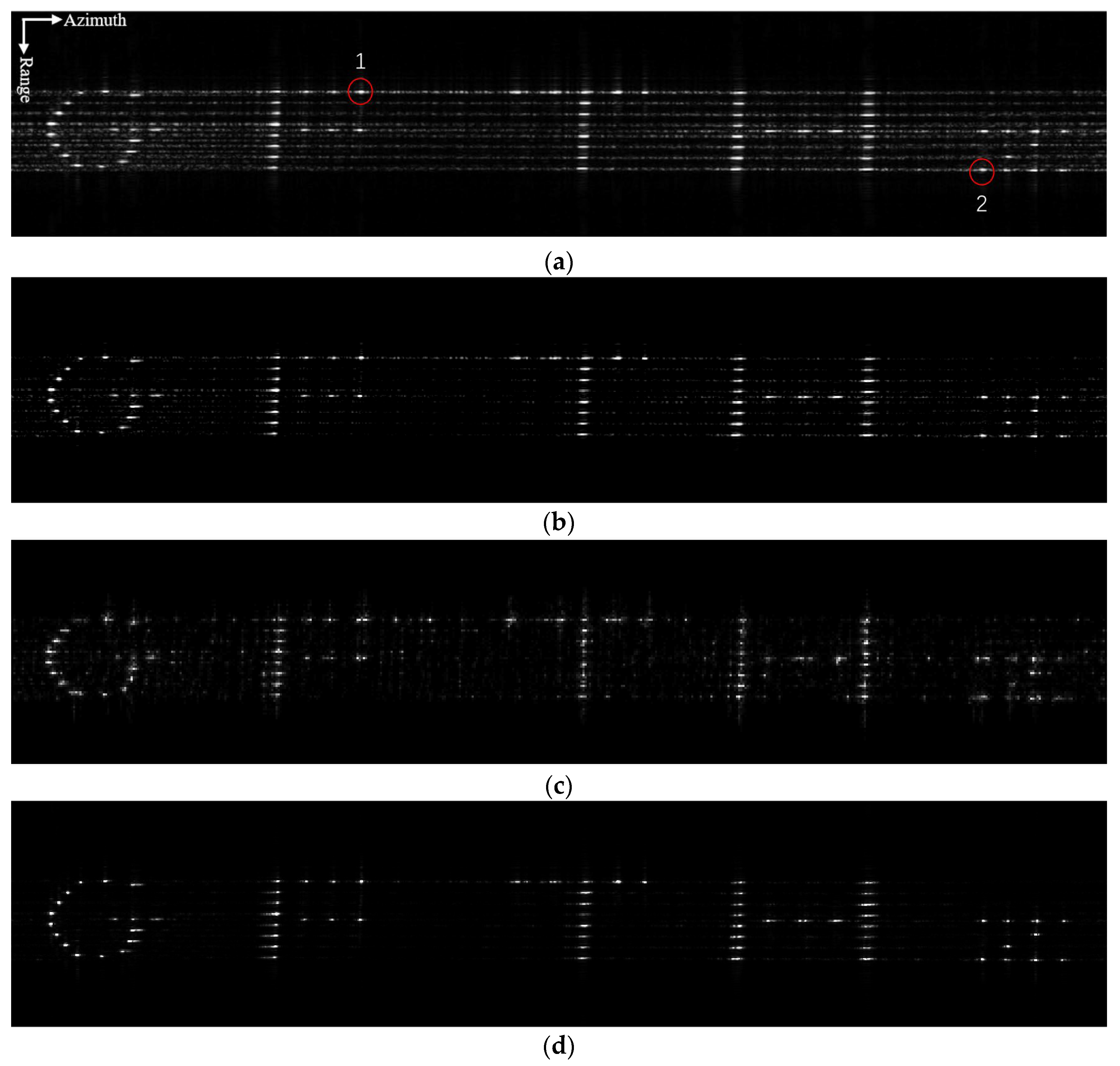
• Experimental Data: Due to the small amount of measured radar data, it is difficult to train the network with measured echoes. Therefore, the network model is trained through using SAR simulation echoes of random point targets and complex surface targets. The specific radar parameter settings used in the training dataset are shown in

  Table 1. SAR system parameters for training data.

  Parameter	Value
  Carrier frequency	9.6 GHz
  Signal bandwidth	60 MHz
  Pulse width	4 μs
  Fast-time sampling	80 MHz
  Synthetic aperture time	1.6 s
  Radar platform velocity	80 m/s
  Pulse repetition frequency	40 Hz

  :

6.

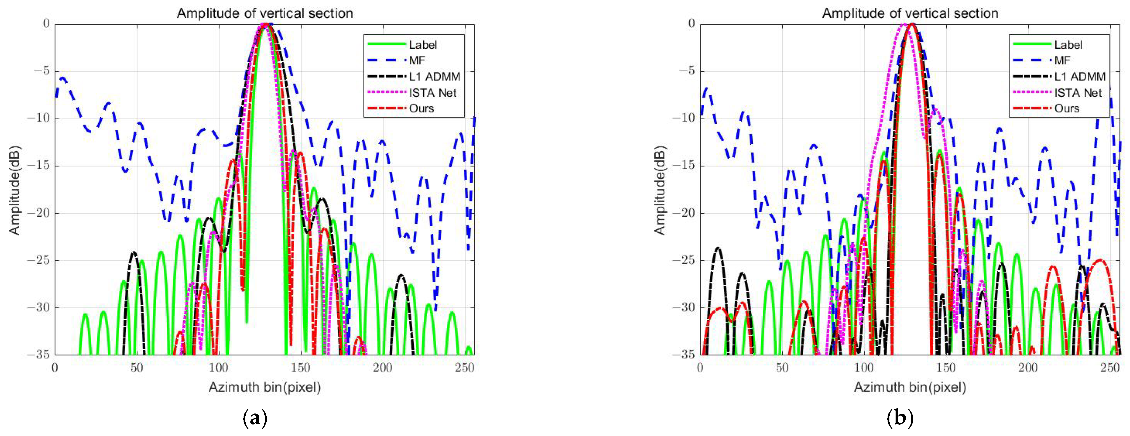
Evaluation Index: For a quantitative evaluation of the reconstruction results, this paper adopts different evaluation criteria according to different scenarios of point targets and surface targets. For the evaluation of the quality of point target reconstruction, some basic point target analysis indexes [38], such as impulse response width (IRW) and peak sidelobe ratio (PSLR), are selected to conduct a quantitative evaluation of the reconstructed point target. In addition, normalized mean square error (NMSE), peak signal-to-noise ratio (PSNR), structural similarity (SSIM), and image entropy (En) are used to evaluate the reconstruction quality of surface targets. Reconstructed image indicators corresponding to surface targets are defined as follows [41]:

$$\mathrm{N}\mathrm{M}\mathrm{S}\mathrm{E}={\displaystyle \frac{{‖{\mathbf{X}}_{\mathrm{r}\mathrm{e}}-{\mathbf{X}}_{\mathrm{l}\mathrm{a}}‖}_{\mathrm{F}}^2}{{‖{\mathbf{X}}_{\mathrm{l}\mathrm{a}}‖}_{\mathrm{F}}^2}}$$

(19)

where ${\mathit{X}}_{re}$ and ${\mathit{X}}_{la}$ are, as described in the previous section, the reconstructed and labeled scenes, respectively. The definition of PSNR is as follows [41]:

$$\mathrm{P}\mathrm{S}\mathrm{N}\mathrm{R}=10{\mathrm{l}\mathrm{o}\mathrm{g}}_{10}\left({\displaystyle \frac{1}{\mathrm{M}\mathrm{S}\mathrm{E}}}\right)$$

(20)

where $\mathrm{M}\mathrm{S}\mathrm{E}={\displaystyle \frac{{‖{\mathbf{X}}_{\mathrm{r}\mathrm{e}}-{\mathbf{X}}_{\mathrm{l}\mathrm{a}}‖}_{\mathrm{F}}^2}{{\mathrm{N}}_{\mathrm{X}}}}$, and $N_X$ is the total number of pixel points in the scene. The definition of SSIM is as follows [41]:

$$\mathrm{S}\mathrm{S}\mathrm{I}\mathrm{M}={\displaystyle \frac{\left(2{\mu }_{{\mathrm{x}}_{\mathrm{r}\mathrm{e}}}{\mu }_{{\mathrm{x}}_{\mathrm{l}\mathrm{a}}}+C_1\right)\left(2{\sigma }_{{\mathrm{x}}_{\mathrm{r}\mathrm{e}}{\mathrm{x}}_{\mathrm{l}\mathrm{a}}}+C_2\right)}{\left({\mu }_{{\mathrm{x}}_{\mathrm{r}\mathrm{e}}}^2+{\mu }_{{\mathrm{x}}_{\mathrm{l}\mathrm{a}}}^2+C_1\right)\left({\sigma }_{{\mathrm{x}}_{\mathrm{r}\mathrm{e}}}^2+{\mathsf{\sigma }}_{{\mathrm{x}}_{\mathrm{l}\mathrm{a}}}^2+C_2\right)}}$$

(21)

where ${\mu }_{{\mathrm{x}}_{\mathrm{r}\mathrm{e}}}$, ${\mu }_{{\mathrm{x}}_{\mathrm{l}\mathrm{a}}}$, ${\sigma }_{{\mathrm{x}}_{\mathrm{r}\mathrm{e}}}$, ${\sigma }_{{\mathrm{x}}_{\mathrm{l}\mathrm{a}}}$, ${\sigma }_{{\mathrm{x}}_{\mathrm{r}\mathrm{e}}{\mathrm{x}}_{\mathrm{l}\mathrm{a}}}$ are the local means, standard deviations, and cross-covariance for images ${\mathbf{X}}_{\mathrm{r}\mathrm{e}}$ and ${\mathbf{X}}_{\mathrm{l}\mathrm{a}}$. $C_1$ and $C_2$ are set as $C_1={{(K}_{1}L)}^2$, $C_2={{(K}_{2}L)}^2$, where $K_1=0.01$, $K_2=0.03$, and L is the range of pixel values of the image, which is set to 0~1.

$$\mathrm{E}\mathrm{n}=-\sum _{i,j}^{I,J}{\displaystyle \frac{{\left|{\mathbf{X}}_{i,j}\right|}^2\log \left({\left|{\mathbf{X}}_{i,j}\right|}^2\right)}{\sum _{i,j}^{I,J}{\left|{\mathbf{X}}_{i,j}\right|}^2}}+\log \left(\sum _{i,j}^{I,J}{\left|{\mathbf{X}}_{i,j}\right|}^2\right)$$

(22)

where $\sum _{i,j}^{I,J}{\left|{\mathbf{X}}_{i,j}\right|}^2$ represents the total energy of the reconstruction result.

For the evaluation of point target image quality, a numerical comparison can be made directly with the theoretical value. For the evaluation of surface targets, this can be known from the definition of index parameters, in which NMSE and PSNR can evaluate the quality of image reconstruction. SSIM represents the advantages and disadvantages of feature reconstruction, and En is used to evaluate the quality of image focusing. The smaller the NMSE and En, the better the image quality; and the larger PSNR and SSIM, the better the image quality.

4. Results

To verify the superiority of the proposed method, we conduct experiments on both simulated and real SAR echo data of different bands. In this article, the traditional MF method (i.e., the Chirp Scaling algorithm), the modified $l_1$-ADMM algorithm, and ISTA-NET are compared with the proposed method. The traditional $l_1$-ADMM brings huge computational costs, which consequently makes the large-scale reconstruction task computationally impossible. And ISAT-NET still needs more iterations when dealing with high-dimensional data or complex scenes. And the performance of the ISAT-NET method depends on the quality and distribution of the training data, which makes it less adaptable to the scene. Therefore, a modified $l_1$-ADMM imaging method combined with a approximate observation operator is used as a comparison method.

4.1. Experiment with Simulation Data

In the simulation experiment, random azimuthal phase errors $\left(-\pi /2,\pi /2\right)$ are added to the echoes, and the reconstruction results under different sampling rates are tested.

In the simulation point target test, we perform echo simulation on some random point target scenes (i.e., these scenes only contain random scattering points, and do not involve the reconstruction of complex surface targets) and use the generated echoes to reconstruct the target scene by different methods, and the reconstruction results are shown in Figure 4.

The specific experimental results are shown in Figure 4. It can be seen from the reconstructed images that the conventional MF method has a defocusing problem under the condition of a sparse azimuth sampling, which leads to the degradation of azimuth resolution, especially under the condition of a low sampling rate. In addition, the image quality is also affected by the error of the surrounding scattering points, resulting in the appearance of false scattering points near the target scattering point. The modified $l_1$-ADMM method can reduce the defocusing problem caused by sparse sampling, but the method is affected by the imaging scene and the algorithm threshold setting. In order to achieve a better processing effect, you need to set different thresholds for different scenarios. Although the ISTA-NET method can handle sparse reconstruction problems, its convergence speed is slow. In sparse sampling scenarios, ISTA is more sensitive to noise and phase errors, and the reconstruction results are prone to artifacts and resolution loss. In contrast, the proposed method can solve the defocusing problems caused by sparse sampling and phase errors. And it does not need to manually set the corresponding threshold.

In order to further analyze the reconstruction effect of different methods, the evaluation indexes, such as PSLR and IRW, are used to analyze the point target in the center right of Figure 4 under different sampling rates. The point target profiles are given in Figure 5, and the specific point target analysis values are shown in

Table 2. Point target performance values comparison under different sampling rates.

Sample	Method	IRW/m [Azimuth]	PSLR/dB [Azimuth]
100%	label	2.6401	−13.2603
20%	MF	5.2509	−5.6680
	$l_1$-ADMM	4.3346	−18.4429
	ISTA-Net	3.0911	−13.5845
	Ours	3.2715	−13.3593
40%	MF	3.6671	−5.6551
	$l_1$-ADMM	3.0002	−23.6377
	ISTA-Net	3.2071	−9.0388
	Ours	2.6147	−13.7778
60%	MF	2.8678	−8.9854
	$l_1$-ADMM	2.5160	−15.6035
	ISTA-Net	3.9686	−6.6601
	Ours	2.6205	−13.1205
80%	MF	2.7052	−10.2679
	$l_1$-ADMM	2.5646	−13.9712
	ISTA-Net	4.3519	−5.9550
	Ours	2.5999	−13.8977

The bold text represents the optimal value under the current sampling rate.

. It can be seen that in the azimuth direction, the image quality of the MF method is seriously degraded due to the phase error and sparse sampling. In particular, with a sampling rate of 20%, its IRW is only 5.4103 m, and the PLSR is −7.2782 dB, which are much different from the theoretical values. As the sampling rate increases, its IRW and PLSR are not up to the theoretical values, although they are improved. Compared with the traditional method, the $l_1$-ADMM method shows some improvement, but there are still defocus issues and even spurious points. Specifically, its IRW improves with the sampling rate, and it meets the requirement when the sampling rate is greater than 60%. In addition, its PLSR is the best in all methods, which shows that $l_1$-ADMM has a better suppression effect on the sidelobes. ISTA-NET’s method gives a better IRW and PSLR at low sampling rates, while when the sampling rate increases, both its IRW and PSLR deteriorate, which may be due to the occurrence of overfitting. For the proposed method, at a sampling rate of 20%, its IRW is closest to the theoretical value of 2.6401 m in all methods, although it does not meet the theoretical resolution requirements, and when the sampling rate is increased to 40%, the IRW meets the requirements. In addition, the PLSR of the proposed method is close to the theoretical value and is basically unaffected by the change in sampling rate. In a word, the proposed method has the best performance.

4.2. Results with Simulation Surface Data

In order to test the adaptability of the network to complex scenarios, the MSAR dataset in [46] is selected to simulate the surface target echo data test. The reconstruction results of different methods are shown in Figure 6, and the image reconstruction is evaluated based on evaluation metrics, such as loss, PSNR, SSIM, and En.

From the results of the surface target simulation data processing, the MF method is affected by phase error and sparse sampling, and the image after processing is seriously defocused, which makes it difficult to distinguish the target. The $l_1$-ADMM method is less affected by the sparse sampling defocus, but the image quality degrades seriously in the presence of phase error. ISTA-NET image quality is better compared to the previous two, but the presence of bokeh can lead to a loss of detail. In addition, the scene reconstructed by the $l_1$-ADMM method is darker, and some weaker target features may be lost in the reconstruction process due to different threshold settings. For example, for the scene at the yellow box in Figure 6, whose partially enlarged image is displayed in Figure 6d, it is difficult to identify its scene targets. In contrast, the proposed method can overcome the influence of phase error in echo well, can reconstruct target features including weak scattering points, and is less affected by a sparse sampling rate.

In order to further analyze the quality of image reconstruction, the imaging results obtained by different reconstruction methods are quantitatively analyzed, and the results are shown in

Table 3. Surface target performance values comparison under different sampling rates.

Sample	Method	Loss	PSNR	SSIM	En
20%	MF	1.5895	28.3058	0.6919	12.1035
	$l_1$-ADMM	0.7336	34.3397	0.6896	8.7402
	ISTA-Net	0.2675	31.2446	0.9400	10.8770
	Ours	0.2103	39.1558	0.9564	10.6137
40%	MF	1.2071	30.2254	0.7549	12.0185
	$l_1$-ADMM	0.6644	34.6875	0.7301	9.1305
	ISTA-Net	0.2317	31.3368	0.9530	10.9314
	Ours	0.2152	40.8972	0.9716	10.5412
60%	MF	1.1441	30.6756	0.7641	12.0557
	$l_1$-ADMM	0.6061	34.5714	0.7533	9.5090
	ISTA-Net	0.2508	31.0499	0.9275	10.7917
	Ours	0.2117	41.9421	0.9779	10.5807
80%	MF	0.8484	32.4294	0.8227	11.9008
	$l_1$-ADMM	0.5602	34.6928	0.7687	9.7558
	ISTA-Net	0.2246	31.2109	0.9695	10.6674
	Ours	0.1644	41.5840	0.9827	10.7998

The bold text represents the optimal value under the current sampling rate.

. In terms of loss, PSNR, and SSIM, the proposed method has the best performance in image feature reconstruction compared with the other three methods. For example, at a sampling rate of 20%, the loss, PSNR, and SSIM are 0.3017, 39.1558 dB, and 0.9564, respectively, which are better than the image reconstruction values of MF,$l_1$-ADMM, and ISTA-NET. Due to the lack of sparse representation ability, the $l_1$-ADMM method ignores background information in the reconstruction process. This may cause the weak scattering targets in scenes not to be reconstructed, which results in the loss of target scene information, causing a decrease in the entropy value of the image. Therefore, the $l_1$-ADMM method has the lowest entropy value in terms of En. In Table 3, the main reason why the image quality of ISTA-Net does not deteriorate with the increase in sampling rate is due to the difference in image sparsity. When the network processes highly sparse images, it can already meet the sparse reconstruction conditions of compressed sensing under low sampling rates, but high sampling will introduce redundant information, resulting in network confusion or overfitting noise, which will degrade the quality. For analysis accuracy, the phase estimation module is analyzed below. The estimated results of the actual phase error and error estimation module are shown in Figure 7. It can be seen from Figure 7a that the phase error estimated by the $\Phi$-module is basically equal to the actual error. Figure 7b shows the estimated error between the two. From the figure, we can see the relative error result after the $\Phi$-module estimates and eliminates the original error. In this case, the residual is only $(-\pi /4,\pi /4)$. The proposed method can effectively suppress the phase error under the limited number of iterations, and the estimated error is within the acceptable range of the actual SAR system, and the imaging effect is obviously better than the existing methods. The residuals can be further optimized by introducing adaptive convergence criteria or higher-order phase models.

In contrast, the proposed method can not only eliminate the defocusing caused by the phase error but also retain scene detail information in the reconstruction process. Therefore, the proposed method has the best reconstruction performance under the comprehensive index.

5. Discussion

5.1. Experiment with Measured Data

In order to verify the effectiveness of the proposed method in this paper, the measured data of different bands are processed. When testing radar-measured data of different bands, it is only necessary to adjust and match the corresponding phase parameter data, rather than train the radar data of different bands one by one. It should be noted that the data size of the training network is fixed, so for data of different specifications, some methods can be used to unify its data size, such as cropping or complementary zero. Specifically, this sampling rate is set to 20%, with some phase error in the azimuth direction.

The SAR data of the stationary ground scene were acquired in Mianyang City, Sichuan Province, China, on June 2011 by the X-band airborne dual-antenna SAR system, which was developed by the Institute of Electronics, Chinese Academy of Sciences. The system parameters for the measured radar data are shown in

Table 4. SAR system parameters in X-band.

Parameter	Value
Carrier frequency	9.6 GHz
Signal bandwidth	492 MHz
Pulse width	13 μs
Fast-time sampling	600 MHz
Synthetic aperture time	0.6 s
Radar platform velocity	105 m/s
Pulse repetition frequency	3125 Hz

.

For the surface target experimental data, three scene echoes are selected for testing, and their experimental results are shown in Figure 8. As can be seen from Figure 8, the image reconstruction quality of the traditional MF method for the three scenes is not good due to the sampling sparsity and phase error. For example, the objects in scenario 1 are indistinguishable, and the objects in scenario 2 appear defocused, reducing the image resolution. Among them, the target outline in scenario 3 is indistinguishable. Compared with the traditional MF method, the $l_1$-ADMM method can reconstruct the target scene to a certain extent, but its reconstruction performance is greatly affected by the empirical threshold. In order not to lose the target feature information, the threshold value for reconstructing the surface target scene should be smaller than that for reconstructing the point target scene, that is, the threshold needs to be set according to the scene type. The ISTA-NET method provides a large improvement in the clarity of imaging over the previous two. The reconstruction effect is even better than the method proposed in this paper in the imaging of scenario 1, but its scene adaptation is poor and the imaging quality in scenario 2 and scenario 3 is degraded. In contrast, the reconstruction performance of the proposed method is best, and one does not need to set the threshold according to the scene type.

In order to quantitatively analyze the reconstruction results of different methods, reconstruction indexes such as PSNR, SSIM and En are given in

Table 5. X-band performance values comparison.

	Method	Loss	PSNR	SSIM	En
Scene 1	MF	0.6742	24.8196	0.7872	12.1657
	$l_1$-ADMM	0.4685	28.2208	0.9068	12.1259
	ISTA-Net	0.2408	30.1058	0.9118	12.0311
	Ours	0.3564	30.0314	0.9201	11.9226
Scene 2	MF	0.3307	29.2021	0.8762	12.0678
	$l_1$-ADMM	0.2128	31.8285	0.9132	11.9612
	ISTA-Net	0.2319	30.7637	0.9152	11.9130
	Ours	0.1765	33.6248	0.9656	11.8108
Scene 3	MF	0.4739	28.6183	0.8667	11.9115
	$l_1$-ADMM	0.2370	32.2342	0.9191	11.6393
	ISTA-Net	0.1721	31.9417	0.9276	11.5030
	Ours	0.1649	35.3073	0.9733	11.3485

The bold text represents the optimal value under the current sampling rate.

. Among them, the proposed method performs better than the other three methods in scenarios 2–3. For example, scenario 3 has the smallest loss and the highest PSNR and SSIM, which are 0.1649, 35.3073, and 0.9733, respectively. And due to the characteristics of ISTA-NET in terms of strong recovery of sparsity, the image loss obtained by ISTA-NET is lower in scenario 1. However, the method proposed in this paper focuses on the robustness of a wide range of scenes and performs more comprehensively in complex scenes. In addition, it can be seen from the entropy value that the entropy of the proposed method is the lowest, which seems to be different from the simulation results. Different from sparse scenarios, in order to obtain richer background information when dealing with complex scenarios, the threshold of $l_1$-ADMM is set lower than the simulation data in the previous section. This also shows that the $l_1$-ADMM method needs parameters to be reset according to different scenes. In contrast, the proposed method does not need the threshold value to be reset but optimizes the parameters during the training process and has a better scene adaptation and robustness compared to ISTA-NET.

5.2. Results with Measured Data in THz Band

To verify the validity of the proposed method, real airborne THz-SAR-measured data were gathered. The data were acquired by the 0.22-THz airborne stripmap SAR system developed by the Beijing Institute of Radio Measurement. The system parameters for the measured radar data are shown in

Table 6. SAR system parameters in THZ band.

Parameter	Value
Carrier frequency	214 GHz
Signal bandwidth	900 MHz
Pulse width	0.15 μs
Fast-time sampling	1.12 GHz
Synthetic aperture time	0.1 s
Radar platform velocity	67 m/s
Pulse repetition frequency	1250 Hz

. The data scene was a GFTHz-shaped real scene consisting of strong scattering point targets.

The experimental results of different methods are shown in Figure 9. As can be seen from Figure 9, the image reconstructed by the traditional MF method has serious defocus in the azimuth, resulting in a decline in image resolution. Compared with the traditional MF method, the $l_1$-ADMM method can improve the imaging effect, but because of the existence of phase error, the image information is destroyed, and some point targets cannot be reconstructed, such as the letters F and T. While the ISTA-NET method is able to reconstruct the image, the target edges are not sharp enough and produce more severe noise, making it difficult to ensure details in the imaging. In contrast, the proposed method has the best effect in image reconstruction. However, it should be noted that the training of the network model in this paper is optimized for a certain range of azimuth phase error. Therefore, the reconstruction effect of the proposed method is not ideal for some point targets with large azimuth phase errors, while the reconstruction effect of the proposed method is good for some point targets with small errors. Therefore, the proposed method is best combined with the error compensation method based on measurement data, so that the imaging effect will be better.

In order to further analyze the imaging quality of the target, the point targets in the red circle in Figure 9. are selected for quantitative analysis, and their profiles and quantitative indexes are shown in Figure 10 and

Table 7. THz-band performance values comparison.

Method	IRW/m		PSLR/dB
	Target 1	Target 2	Target 1	Target 2
Theory	0.0998		−13.2600
MF	0.1662	0.2104	−9.7297	−8.6605
$l_1$-ADMM	0.1506	0.1680	−11.9509	−11.1654
ISTA-NET	0.0850	0.1891	−2.8339	−2.2068
Ours	0.0999	0.1035	−15.9870	−11.3810

The bold text represents the optimal value under the current sampling rate.

, respectively. It can be seen that for point target 2, the IRW and PSLR of the MF method are 0.2104 and −8.6605 dB, respectively, which are significantly different from the theoretical values of 0.0998 and 13.2600. In addition, the IRW and PLSR of the $l_1$-ADMM method are improved compared with the MF method, being 0.1610 and −11.1654 dB, respectively, but they do not reach the theoretical value. The IRW and PSLR of ISTA-NET show deterioration compared to the $l_1$-ADMM algorithm, being 0.1891 and −2.2068 dB, respectively, which can lead to severe detail loss. In contrast, the IRW and PSLR of the proposed method agree well with the theoretical values, which proves the effectiveness of the proposed method in sparse imaging and error compensation. This is because the design idea of modular separation in this paper significantly reduces the computational complexity and improves the generalization ability for radar systems in different bands, while retaining the efficiency of traditional imaging algorithms (such as CS). By introducing $L_p$ regularization, the algorithm can automatically optimize parameters through end-to-end training, thus reducing the dependence on manual parameter tuning. Therefore, compared with traditional methods, the algorithm proposed in this paper uses data-driven self-optimization parameters to improve the robustness and adaptability of imaging in different scenes and different bands. The suboptimal parameters brought by manual parameter adjustment are avoided. Despite the above advantages, this method still has some defects. When processing images with large phase errors, the current phase error compensation module will have a large error. At the same time, there is a high demand for data and computing power in the training stage. If there is any problem with the training data, the imaging results will be greatly affected.

6. Conclusions

To solve the problem that existing sparse SAR imaging networks have a poor adaptive ability in different bands, a novel deep unfolding network for multi-band SAR sparse imaging and autofocusing based on approximate observation is proposed. Firstly, the approximate observation operator module is designed separately from the sparse imaging optimization network to adapt to radar systems of different bands. Compared with the fixed $l_1$ regularization, the proposed method adopts network training to achieve an adaptive optimization based on $l_p$ parameters to characterize the uncertain transformation domain of the target scene, which has a better reconstruction effect for complex scenes. In view of the phase errors that may be introduced in the SAR echo acquisition process, an error compensation module is added in the imaging optimization process, and the imaging and autofocusing of the target scene are realized at the same time. Finally, airborne SAR simulation and real imaging experiments in the 0.22 THz and 9.6 GHz bands are performed to verify the effectiveness of the proposed method in multi-band scenarios. In the experiment, four sparse levels of 20%, 40%, 60%, and 80% are used to compare and analyze the imaging performance of different methods in complex scenes. The results show that the proposed method is superior to the existing methods in key evaluation indexes such as loss, PSNR, SSIM, and En. In summary, the deep spread network proposed in this paper has significant advantages in the sparse imaging and self-focusing of multi-band SAR. The introduction of approximate observation operators and $P$ operators realizes a dynamic adaptation to different band radar systems and different scenes and successfully reduces the dependence on manual parameter tuning. The introduction of a phase error compensation module further enhances the robustness of the algorithm in low sampling rate and strong noise environments, and it provides a more efficient and reliable solution for the practical application of multi-band and multi-scene SAR.

The proposed method has high training requirements for imaging and incurs a significant computational cost. In addition, the shortcoming of the proposed method is that the current phase error compensation module can only estimate and compensate for a small range of phase errors, and it cannot well estimate and compensate for a large range of errors. In the future, it is necessary to add a larger range of more complex errors in the network-training process, so as to realize the estimation of and compensation for arbitrary errors. For example, the incorporation of an adaptive convergence criterion or a higher-order phase model can further optimize the phase error.