Bayesian FDOA Positioning with Correlated Measurement Noise

Abstract

In this paper, the problem of source localization using only frequency difference of arrival (FDOA) measurements is considered. A new FDOA-only localization technique is developed to determine the position of a narrow-band source. In this scenario, time difference of arrival (TDOA) measurements are not normally useful because they may have large errors due to the received signal having a small bandwidth. Conventional localization algorithms such as the two-stage weighted least squares (TSWLS) method, which jointly exploits TDOA and FDOA measurements for positioning, are thus no longer applicable since they will suffer from the thresholding effect and yield meaningless localization results. FDOA-only localization is non-trivial, mainly due to the high nonlinearity inherent in FDOA equations. Even with two FDOA measurements being available, FDOA-only localization still requires finding the roots of a high-order polynomial. For practical scenarios with more sensors, a divide-and-conquer (DAC) approach may be applied, but the positioning solution is suboptimal due to ignoring the correlation between FDOA measurements. To address these challenges, in this work, we propose a Bayesian approach for FDOA-only source positioning. The developed method, referred to as the Gaussian division method (GDM), first converts one FDOA measurement into a Gaussian mixture model (GMM) that specifies the prior distribution of the source position. Next, the GDM assumes uncorrelated FDOA measurements and fuses the remaining FDOAs sequentially by invoking nonlinear filtering techniques to obtain an initial positioning result. The GDM refines the solution by taking into account and compensating for the information loss caused by ignoring that the FDOAs are in fact correlated. Extensive simulations demonstrate that the proposed algorithm provides improved performance over existing methods and that it can attain the Cramér–Rao lower bound (CRLB) accuracy under moderate noise levels.

1. Introduction

Passive localization refers to determining the source position without transmitting illuminating signals. It relies solely on analyzing the signals emitted by the source to estimate its location, and it has advantages such as good concealment and a large coverage area. Passive localization has wide applications in diverse areas, including but not limited to wireless communications, navigation, surveillance, and search and rescue [1,2,3,4,5].

Currently, passive localization systems typically exploit one or more types of signal measurements, such as the angle of arrival (AOA)  [6,7,8], received signal strength (RSS) [9,10,11], time of arrival (TOA) [12,13,14], phase difference of arrival (PDOA) [15,16,17], TDOA [18,19,20], and FDOA [21,22,23], to locate the source of interest. Among them, TDOA-FDOA localization is an effective scheme, generally involving the use of multiple moving observers [24,25,26,27,28]. The system captures the signals from the source and computes the cross-ambiguity function (CAF) between the signals received at different observers to extract the desired TDOA and FDOA measurements [29]. Subsequently, techniques like the TSWLS method [30,31] can be employed for positioning. Although this scheme is capable of accurately locating wide-band sources, its performance may greatly deteriorate for narrow-band sources. The underlying reason is that the measurement error of TDOA is inversely proportional to the signal bandwidth [32]. When the source signal is band-limited, TDOA measurement errors increase significantly, which could render the conventional TDOA-FDOA positioning algorithms no longer applicable due to the thresholding effect. However, FDOA measurements are usually still useful in this case, because the FDOA measurement noise can be mitigated by increasing the measurement interval [33]. FDOA-only localization thus becomes critical for source localization in the absence of TDOAs [34].

FDOA measurements are related to the unknown source position in a highly nonlinear manner. This strong nonlinearity makes FDOA-only positioning a nontrivial task. In the literature, efforts have been made to find a reliable way to address this problem. Specifically, when three observers are present, two FDOAs are available for positioning. In this case, the problem can be cast into finding the intersection point of the two curves specified by the two FDOA measurements. This requires finding the roots of a 22nd-order polynomial [35]. This root finding-based approach is numerically challenging and, moreover, difficult to extend to more general scenarios with four or more observers. However, the FDOA-random-sample-consensus (FDOAR) algorithm [36] utilizes a pair of carefully selected FDOA measurements to find the source position estimate, while the location information from other measurements is simply discarded. The Gauss–Newton (GN) iterative algorithm in [37] requires a good initial solution guess of the source position, but this may not be easily obtained in many scenarios. Closed-form solutions [38,39] derived from pseudo-linearizing the FDOA measurement equations also exist. However, due to the introduction of quite a few nuisance parameters, the method is only applicable when the number of observers is sufficiently large so as to guarantee the identifiability of all the unknowns. This significantly limits their practical applications. Geometric methods [40,41,42], which determine the source position by intersecting iso-FDOA curves (i.e., the loci of constant FDOA) in Cartesian or polar coordinate systems, offer lower precision compared to other approaches.

Bayesian filtering techniques such as those developed in [43] are readily available for solving nonlinear target tracking problems. We follow a similar idea and adapt Bayesian inference to tackle the FDOA-only localization task. The developed algorithm, called the GDM, first finds a GMM representation of the prior distribution of the source position based on one of the FDOA measurements. This explores the universal approximation capability of the GMM to achieve good coverage of the irregular area of interest specified by one FDOA [44]. Next, the GDM updates the GMM by fusing the remaining FDOA measurements to accomplish the desired localization. This is achieved in two steps. In the first step, the correlation between the FDOAs is neglected to facilitate the sequential processing of the measurements by invoking standard nonlinear filtering techniques. The second step refines the initial positioning result by taking into account the fact that the FDOA measurements are in fact correlated.

The proposed algorithm offers several key advantages:

(1)

It addresses the FDOA-only localization problem using a Bayesian inference framework, circumventing the need to find roots for high-order polynomials and therefore avoiding spurious solutions. Our approach utilizes a GMM representation of the prior distribution of the source position, which eliminates the requirement of obtaining good initial estimates, as in common iterative methods.

(2)

The algorithm does not introduce any nuisance parameters and can thus be employed directly in scenarios with three or more observers.

(3)

Empirical results confirm that, at low and moderate noise levels, the proposed method attains performance closely approaching the CRLB.

The remainder of this paper is organized as follows: Section 2 describes the localization problem considered. Section 3 proposes the Bayesian positioning method, namely, the GDM algorithm. Section 4 presents the GMM initialization process. Section 5 analyzes the algorithm’s performance, and Section 6 evaluates our algorithm’s performance via simulation experiments. Finally, Section 7 concludes this work.

2. Problem Formulation

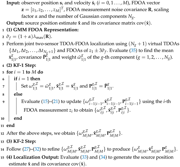
Consider the FDOA-only localization problem shown in Figure 1. Any point on an iso-FDOA curve can produce the same true FDOA. Thus, it corresponds to the set of locations that the source must lie in. The system has $M+1$ moving observers for locating a stationary source on the two-dimensional (2D) plane. The true source position $\mathbf{x}={[x_t,y_t]}^T$ is to be estimated. Due to the relative motion between the source and the observers, the signal received at the i-th observer that is located at ${\mathbf{s}}_i={[x_i,y_i]}^T$ and moving with a velocity of ${\dot{\mathbf{s}}}_i={[{\dot{x}}_i,{\dot{y}}_i]}^T$, $i=0,1,\dots ,M$ experiences a Doppler shift equal to

$$f_i^o\left(\mathbf{x}\right)={\displaystyle \frac{f_c}{c}}{\mathbf{r}}_i^T\left(\mathbf{x}\right){\dot{\mathbf{s}}}_i.$$

(1)

where c is the signal propagation speed, $f_c$ denotes the carrier frequency of the source signal, and ${\mathbf{r}}_i\left(\mathbf{x}\right)$ is the line-of-sight (LOS) vector pointing from the i-th observer ${\mathbf{s}}_i$ to the source $\mathbf{x}$, i.e.,

$$\begin{array}{cc}\hfill & {\mathbf{r}}_i\left(\mathbf{x}\right)=(\mathbf{x}-{\mathbf{s}}_i)/r_i\left(\mathbf{x}\right),\hfill \end{array}$$

(2a)

$$\begin{array}{cc}\hfill & r_i\left(\mathbf{x}\right)=\parallel \mathbf{x}-{\mathbf{s}}_i\parallel ,\hfill \end{array}$$

(2b)

where the notation $\parallel ·\parallel$ represents the Euclidean norm.

Without the loss of generality, we designate the first observer as the reference observer ${\mathbf{s}}_0$ such that the FDOA measurement between the i-th and the reference observer, denoted as $z_i$ ($i=1,2,\dots ,M$), can be written as

$$\begin{array}{cc}\hfill & z_i=h_i\left(\mathbf{x}\right)+n_i,\hfill \end{array}$$

(3a)

$$\begin{array}{cc}\hfill & h_i\left(\mathbf{x}\right)=f_i^o\left(\mathbf{x}\right)-f_0^o\left(\mathbf{x}\right),\hfill \end{array}$$

(3b)

where $n_i$ is the additive measurement noise assumed to be a zero-mean Gaussian random variable.

Stacking the M FDOA measurements yields

$$\mathbf{z}=\mathbf{h}\left(\mathbf{x}\right)+\mathbf{n},$$

(4)

where $\mathbf{z}={[z_1,z_2,\cdots ,z_M]}^T$, $\mathbf{h}\left(\mathbf{x}\right)={[h_1\left(\mathbf{x}\right),h_2\left(\mathbf{x}\right),\cdots ,h_M\left(\mathbf{x}\right)]}^T$, and $\mathbf{n}={[n_1,n_2,\cdots ,n_M]}^T$. The noise vector follows a multivariate Gaussian distribution with zero mean and covariance matrix $\mathbf{R}\in {\mathbb{R}}^{M\times M}$ being equal to [31]

$$\mathbf{R}=\mathbb{E}\left[\mathbf{n}{\mathbf{n}}^T\right]={\sigma }_f^2\left[\begin{array}{cccc}1& 0.5& \cdots & 0.5\\ 0.5& 1& \cdots & 0.5\\ ⋮& ⋮& \ddots & ⋮\\ 0.5& 0.5& \cdots & 1\end{array}\right],$$

(5)

where ${\sigma }_f$ is the noise standard deviation. It can be seen in (5) that the noise covariance $\mathbf{R}$ has non-zero off-diagonal elements. This indicates that the FDOA measurements are actually correlated. The correlation comes from the subtraction needed to form FDOAs (see (3b)), which causes the Doppler measurement noise at the reference observer ${\mathbf{s}}_0$ to be shared by all the FDOAs.

By using the fact that the measurement vector $\mathbf{z}$ is Gaussian-distributed with mean $\mathbf{h}\left(\mathbf{x}\right)$ and covariance $\mathbf{R}$, the FDOA-only localization can be realized by solving the following maximum likelihood estimation (MLE) problem:

$$\widehat{\mathbf{x}}=\underset{\mathbf{x}}{argmin}{(\mathbf{z}-\mathbf{h}\left(\mathbf{x}\right))}^T{\mathbf{R}}^{-1}(\mathbf{z}-\mathbf{h}\left(\mathbf{x}\right)).$$

(6)

where $\widehat{\mathbf{x}}$ denotes the source position estimate.

The optimization problem in (6) does not admit a closed-form solution because the FDOA measurement functions $h_i\left(\mathbf{x}\right)$ are highly nonlinear with respect to the unknown source position $\mathbf{x}$. To address this difficulty, in the next section, we develop a Bayesian localization method. This approach also accounts for the correlated nature of measurement noise.

3. Bayesian FDOA-Only Localization

In this section, we introduce the proposed Bayesian FDOA-only localization algorithm, the GDM. From the Bayesian perspective, the source position estimate can be found by computing the mean of the source position posterior $p\left(\mathbf{x}\right|\mathbf{z})$. That is, $\widehat{\mathbf{x}}$ is now equal to

$$\widehat{\mathbf{x}}\approx \int \mathbf{x}p\left(\mathbf{x}\right|\mathbf{z})d\mathbf{x}.$$

(7)

The key task of Bayesian FDOA-only localization then reduces to finding the posterior $p\left(\mathbf{x}\right|\mathbf{z})$.

By Bayes’ theorem, the posterior distribution $p\left(\mathbf{x}\right|\mathbf{z})$ is

$$\begin{array}{cc}\hfill & p\left(\mathbf{x}\right|\mathbf{z})\propto p(\mathbf{z}\left|\mathbf{x}\right)p\left(\mathbf{x}\right),\hfill \end{array}$$

(8a)

$$\begin{array}{cc}\hfill & p\left(\mathbf{z}\right|\mathbf{x})=\mathcal{N}(\mathbf{z};\mathbf{h}\left(\mathbf{x}\right),\mathbf{R}),\hfill \end{array}$$

(8b)

where $p\left(\mathbf{x}\right)$ denotes the prior distribution of the source position $\mathbf{x}$, and $p\left(\mathbf{z}\right|\mathbf{x})$ is the FDOA measurement likelihood. $\mathcal{N}(\mathbf{x};\mathit{\mu },\mathit{S})$ indicates that $\mathbf{x}$ is Gaussian-distributed with mean $\mathit{\mu }$ and covariance $\mathit{S}$.

To evaluate (8a), we need to specify the prior distribution $p\left(\mathbf{x}\right)$ first. Fortunately, we can exploit the notion that the source should be located with a high probability close to 1 in the $\pm 3\sigma$ region of the iso-FDOA curve determined by any FDOA measurement. We thus utilize the FDOA measurement $z_1$ to derive the desired source position prior $p\left(\mathbf{x}\right)$. In particular, $p\left(\mathbf{x}\right)$ is represented using a GMM model. Details on this initialization process can be found in the next section, Section 4.

Mathematically, the source position prior $p\left(\mathbf{x}\right)$ can now be re-written as

$$\overline{p}\left(\mathbf{x}|z_1\right)=\sum _{g=1}^{N_g}{\overline{\omega }}_{1|1}^g\mathcal{N}\left(\mathbf{x};{\overline{\mathbf{x}}}_{1|1}^g,{\overline{\mathbf{P}}}_{1|1}^g\right).$$

(9)

It is in fact the posterior of the source position given by the FDOA measurement $z_1$. $\overline{p}\left(\mathbf{x}|z_1\right)$ is essentially a weighted sum of $N_g$ Gaussian components. The g-th Gaussian component has mean ${\overline{\mathbf{x}}}_{1|1}^g$, covariance ${\overline{\mathbf{P}}}_{1|1}^g$, and weight ${\overline{\omega }}_{1|1}^g$, where ${\overline{\omega }}_{1|1}^g>0$ and ${\sum }_{g=1}^{N_g}{\overline{\omega }}_{1|1}^g=1$.

By replacing $p\left(\mathbf{x}\right)$ with $\overline{p}\left(\mathbf{x}|z_1\right)$, the desired source position posterior in (8a) may be found by invoking nonlinear filtering techniques. This is achieved in two steps. In the first step, it is assumed that the FDOA measurements are uncorrelated with a diagonal covariance. This enables the fusion of the available FDOAs in a sequential manner. Simulation experiments show that a good initial source position estimate can indeed be obtained. In the second step, the initial localization result is updated by compensating for the information loss caused by ignoring the measurement correlation. This design is flexible and scalable in the sense that, if the number of observers is large, we may carry out the first step only but still attain a good localization output with low computational burden. If the computational resource allows, the second step can be executed for improved performance.

The algorithm development starts with defining $\mathcal{I}$ as an auxiliary variable to indicate that the measurements collected in $\mathbf{z}$ are assumed to be independently distributed. We then introduce a pseudo-likelihood $p\left(\mathbf{z}\right|\mathbf{x},\mathcal{I})$ into (8a) to arrive at

$$\begin{array}{cc}\hfill p\left(\mathbf{x}\right|\mathbf{z})& \propto {\displaystyle \frac{p\left(\mathbf{z}\right|\mathbf{x})}{p\left(\mathbf{z}\right|\mathbf{x},\mathcal{I})}}p\left(\mathbf{z}\right|\mathbf{x},\mathcal{I})p\left(\mathbf{x}\right)\hfill \\ & \propto {\displaystyle \frac{p\left(\mathbf{z}\right|\mathbf{x})}{p\left(\mathbf{z}\right|\mathbf{x},\mathcal{I})}}p\left(\mathbf{x}\right|\mathbf{z},\mathcal{I})p\left(\mathbf{z}\right|\mathcal{I})\hfill \\ \hfill & \propto {\displaystyle \frac{p\left(\mathbf{z}\right|\mathbf{x})}{p\left(\mathbf{z}\right|\mathbf{x},\mathcal{I})}}p\left(\mathbf{x}\right|\mathbf{z},\mathcal{I}).\hfill \end{array}$$

(10)

This implies that the proposed algorithm first finds the source position posterior $p\left(\mathbf{x}\right|\mathbf{z},\mathcal{I})$ under the assumption that the FDOAs are uncorrelated and then refines it using the likelihood ratio ${\displaystyle \frac{p\left(\mathbf{z}\right|\mathbf{x})}{p\left(\mathbf{z}\right|\mathbf{x},\mathcal{I})}}$.

One possible choice for the pseudo-likelihood $p\left(\mathbf{z}\right|\mathbf{x},\mathcal{I})$ is a multivariate Gaussian distribution with the same mean as the true likelihood $p\left(\mathbf{z}\right|\mathbf{x})$ but a diagonal covariance. More specifically, we set

$$\begin{array}{cc}\hfill & p\left(\mathbf{z}\right|\mathbf{x},\mathcal{I})=\mathcal{N}(\mathbf{z};\mathbf{h}\left(\mathbf{x}\right),\mathbf{D}),\hfill \end{array}$$

(11a)

$$\begin{array}{cc}\hfill & \mathbf{D}={\widehat{\sigma }}_f^2·{\mathbf{I}}_M,\hfill \end{array}$$

(11b)

where ${\widehat{\sigma }}_f$ (${\widehat{\sigma }}_f\ne {\sigma }_f$) is the assumed FDOA measurement noise standard deviation, and ${\mathbf{I}}_M$ represents an $M\times M$ identity matrix. The selection of ${\widehat{\sigma }}_f$ is discussed at the end of Section 3.2. Due to the diagonal structure of the covariance matrix $\mathbf{D}$, the pseudo-likelihood $p\left(\mathbf{z}\right|\mathbf{x},\mathcal{I})$ can be factorized into

$$p\left(\mathbf{z}\right|\mathbf{x},\mathcal{I})=\prod _{i=1}^{M}p\left(z_i\right|\mathbf{x},\mathcal{I})=\prod _{i=1}^M\mathcal{N}(z_i;h_i\left(\mathbf{x}\right),{\widehat{\sigma }}_f^2).$$

(12)

3.1. KF-1 Step: Evaluating $p\left(\mathbf{x}\right|\mathbf{z},\mathcal{I})$

Again, by Bayes’ theorem, $p\left(\mathbf{x}\right|\mathbf{z},\mathcal{I})$ can be expressed as

$$\begin{array}{cc}\hfill p\left(\mathbf{x}|\mathbf{z},\mathcal{I}\right)& =p\left(\mathbf{x}|z_M,\cdots ,z_2,z_1,\mathcal{I}\right)\hfill \\ \hfill & ={\displaystyle \frac{p\left(z_M,\cdots ,z_2|\mathbf{x},z_1,\mathcal{I}\right)p\left(\mathbf{x}|z_1,\mathcal{I}\right)}{p\left(z_M,\cdots ,z_2|z_1,\mathcal{I}\right)}}\hfill \\ \hfill & \propto \prod _{i=2}^{M}p\left(z_i|\mathbf{x},\mathcal{I}\right)\overline{p}\left(\mathbf{x}\right|z_1,\mathcal{I}).\hfill \end{array}$$

(13)

It is important to point out that, when computing the source posterior $p\left(\mathbf{x}\right|\mathbf{z},\mathcal{I})$ using (13), the source position prior $\overline{p}\left(\mathbf{x}\right|z_1,\mathcal{I})$ still takes the form of a GMM model as in (9), which is derived using the initialization method in Section 4, but, in this case, the FDOA $z_1$ has the assumed variance ${\widehat{\sigma }}_f^2$ instead of ${\sigma }_f^2$. This will also be compensated in the second step of the proposed algorithm (see Section 3.2).

After putting ${\omega }_{1|1}^{g,\mathcal{I}}={\overline{\omega }}_{1|1}^g$, ${\widehat{\mathbf{x}}}_{1|1}^{g,\mathcal{I}}={\overline{\mathbf{x}}}_{1|1}^g$, and ${\mathbf{P}}_{1|1}^{g,\mathcal{I}}={\overline{\mathbf{P}}}_{1|1}^g$, we substitute (9) and express (13) as

$$\begin{array}{cc}\hfill p\left(\mathbf{x}|\mathbf{z},\mathcal{I}\right)& \propto \sum _{g=1}^{N_g}{\omega }_{1|1}^{g,\mathcal{I}}\prod _{i=2}^M\mathcal{N}(z_i;h_i\left(\mathbf{x}\right),{\widehat{\sigma }}_f^2)\mathcal{N}(\mathbf{x};{\widehat{\mathbf{x}}}_{1|1}^{g,\mathcal{I}},{\mathbf{P}}_{1|1}^{g,\mathcal{I}})\hfill \\ \hfill & =\sum _{g=1}^{N_g}{\omega }_{M|M}^{g,\mathcal{I}}\mathcal{N}(\mathbf{x};{\widehat{\mathbf{x}}}_{M|M}^{g,\mathcal{I}},{\mathbf{P}}_{M|M}^{g,\mathcal{I}}).\hfill \end{array}$$

(14)

The second equality can be realized by invoking one standard nonlinear filtering technique to fuse the FDOA measurements sequentially. The desired source position posterior $p\left(\mathbf{x}\right|\mathbf{z},\mathcal{I})$ takes the form of a GMM model, as the source position prior.

For completeness, in the following, the detailed computation procedure for finding the triplet $\{{\omega }_{M|M}^{g,\mathcal{I}},{\widehat{\mathbf{x}}}_{M|M}^{g,\mathcal{I}},{\mathbf{P}}_{M|M}^{g,\mathcal{I}}\}$ in (14) in a sequential manner is given. The cubature Kalman filter (CKF) originally developed in [45] is used for nonlinear filtering.

Suppose that we have fused the first $(i-1)$ FDOA measurements. The source position posterior has the same functional form as in (14) but with triplet $\{{\omega }_{i-1|i-1}^{g,\mathcal{I}},{\widehat{\mathbf{x}}}_{i-1|i-1}^{g,\mathcal{I}},{\mathbf{P}}_{i-1|i-1}^{g,\mathcal{I}}\}$. We proceed to explore the i-th FDOA to update the triplet of the source position posterior. We denote the updated triplet using $\{{\omega }_{i|i}^{g,\mathcal{I}},{\widehat{\mathbf{x}}}_{i|i}^{g,\mathcal{I}},{\mathbf{P}}_{i|i}^{g,\mathcal{I}}\}$. The process follows the prediction–correction framework.

(1)

State prediction:

$$\begin{array}{cc}\hfill {\widehat{\mathbf{x}}}_{i|i-1}^{g,\mathcal{I}}& ={\widehat{\mathbf{x}}}_{i-1|i-1}^{g,\mathcal{I}},g=1,2,\dots ,N_g,\hfill \end{array}$$

(15a)

$$\begin{array}{cc}\hfill {\mathbf{P}}_{i|i-1}^{g,\mathcal{I}}& ={\mathbf{P}}_{i-1|i-1}^{g,\mathcal{I}},g=1,2,\dots ,N_g,\hfill \end{array}$$

(15b)

where ${\widehat{\mathbf{x}}}_{i|i-1}^{g,\mathcal{I}}$ and ${\mathbf{P}}_{i|i-1}^{g,\mathcal{I}}$ denote the predicted mean and covariance of the g-th Gaussian component. The above state prediction comes from that in the considered localization problem, and the source is stationary. Let $\sqrt{{\mathbf{P}}_{i|i-1}^{g,\mathcal{I}}}$ be the Cholesky decomposition of ${\mathbf{P}}_{i|i-1}^{g,\mathcal{I}}$ such that $\left(\sqrt{{\mathbf{P}}_{i|i-1}^{g,\mathcal{I}}}\right){\left(\sqrt{{\mathbf{P}}_{i|i-1}^{g,\mathcal{I}}}\right)}^T={\mathbf{P}}_{i|i-1}^{g,\mathcal{I}}$.

(2)

Cubature point generation:

$${\mathbf{X}}_{k,i|i-1}^{g,\mathcal{I}}=\sqrt{{\mathbf{P}}_{i|i-1}^{g,\mathcal{I}}}{\mathbf{\xi }}_k+{\widehat{\mathbf{x}}}_{i|i-1}^{g,\mathcal{I}},g=1,2,\dots ,N_g,k=1,2,\dots ,2n_x,$$

(16)

where ${\mathbf{\xi }}_k$ denotes the k-th cubature point. According to [45], it is the k-th column of matrix $\sqrt{n_x}[{\mathbf{I}}_{n_x},-{\mathbf{I}}_{n_x}]$, where ${\mathbf{I}}_{n_x}$ is an $n_x\times n_x$ identity matrix, and $n_x$ ($n_x=2$ for the considered 2D localization problem) denotes the dimension of the unknown source position vector $\mathbf{x}$.

(3)

Cubature point propagation:

$$z_{k,i|i-1}^g=h_i\left({\mathbf{X}}_{k,i|i-1}^{g,\mathcal{I}}\right),g=1,2,\dots ,N_g,k=1,2,\dots ,2n_x,$$

(17)

where ${\mathbf{X}}_{k,i|i-1}^{g,\mathcal{I}}$ is the transformed cubature point in (16), and $h_i(·)$ is the i-th FDOA measurement function defined in (3b).

(4)

FDOA measurement prediction:

$${\widehat{z}}_{i|i-1}^g={\displaystyle \frac{1}{2n_x}}\sum _{k=1}^{2n_x}{z}_{k,i|i-1}^g,g=1,2,\dots ,N_g,$$

(18)

where $z_{k,i|i-1}^g$ is the propagated cubature point in (17).

(5)

Kalman gain computation:

$$\begin{array}{cc}\hfill & {\sigma }_{zz,i|i-1}^{g,2}={\displaystyle \frac{1}{2n_x}}\sum _{k=1}^{2n_x}{(z_{k,i|i-1}^g-{\widehat{z}}_{i|i-1}^g)}^2+{\widehat{\sigma }}_f^2,\hfill \end{array}$$

(19a)

$$\begin{array}{cc}\hfill & {\mathbf{P}}_{xz,i|i-1}^g={\displaystyle \frac{1}{2n_x}}\sum _{k=1}^{2n_x}(z_{k,i|i-1}^g-{\widehat{z}}_{i|i-1}^g)({\mathbf{X}}_{k,i|i-1}^{g,\mathcal{I}}-{\widehat{\mathbf{x}}}_{i|i-1}^{g,\mathcal{I}}),\hfill \end{array}$$

(19b)

$$\begin{array}{cc}\hfill & {\mathbf{K}}_{i|i-1}^g={\displaystyle \frac{1}{{\sigma }_{zz,i|i-1}^{g,2}}}{\mathbf{P}}_{xz,i|i-1}^g,\hfill \end{array}$$

(19c)

where $z_{k,i|i-1}^g$ is the propagated cubature point in (17), ${\widehat{z}}_{i|i-1}^g$ is the predicted FDOA measurement in (18), ${\widehat{\sigma }}_f$ is the assumed FDOA measurement noise standard deviation defined in (11b), ${\mathbf{X}}_{k,i|i-1}^{g,\mathcal{I}}$ is the transformed cubature point in (16), and ${\widehat{\mathbf{x}}}_{i|i-1}^{g,\mathcal{I}}$ is the predicted state vector given in (15a).

(6)

Mean and covariance update:

$$\begin{array}{cc}\hfill & {\widehat{\mathbf{x}}}_{i|i}^{g,\mathcal{I}}={\widehat{\mathbf{x}}}_{i|i-1}^{g,\mathcal{I}}+{\mathbf{K}}_{i|i-1}^g(z_i-{\widehat{z}}_{i|i-1}^g),g=1,2,\dots ,N_g,\hfill \end{array}$$

(20a)

$$\begin{array}{cc}& {\mathbf{P}}_{i|i}^{g,\mathcal{I}}={\mathbf{P}}_{i|i-1}^{g,\mathcal{I}}-{\sigma }_{zz,i|i-1}^{g,2}{\mathbf{K}}_{i|i-1}^g{\left({\mathbf{K}}_{i|i-1}^g\right)}^T,g=1,2,\dots ,N_g,\hfill \end{array}$$

(20b)

where $z_i$ is the i-th FDOA measurement. The above equations update the predicted mean and covariance $\{{\widehat{\mathbf{x}}}_{i|i-1}^{g,\mathcal{I}},{\mathbf{P}}_{i|i-1}^{g,\mathcal{I}}\}$ to $\{{\widehat{\mathbf{x}}}_{i|i}^{g,\mathcal{I}},{\mathbf{P}}_{i|i}^{g,\mathcal{I}}\}$ using the Kalman gain ${\mathbf{K}}_{i|i-1}^g$ in (19c), the predicted FDOA measurement ${\widehat{z}}_{i|i-1}^g$ in (18), and the innovation variance ${\sigma }_{zz,i|i-1}^{g,2}$ in (19a).

(7)

Component weight update:

$${\omega }_{i|i}^{g,\mathcal{I}}\propto {\omega }_{i|i-1}^{g,\mathcal{I}}·\mathcal{N}(z_i,{\widehat{z}}_{i|i-1}^g,{\sigma }_{zz,i|i-1}^{g,2}),$$

(21)

Here, ${\sigma }_{zz,i|i-1}^{g,2}$ is the innovation variance given in (19a). The component weight ${\omega }_{i|i}^{g,\mathcal{I}}$ needs to be normalized such that ${\sum }_{i=1}^{N_g}{\omega }_{i|i}^{g,\mathcal{I}}=1$.

So far, we have shown in (15)–(21) how the algorithm fuses one FDOA measurement. The above process starts with $\{{\omega }_{1|1}^{g,\mathcal{I}},{\widehat{\mathbf{x}}}_{1|1}^{g,\mathcal{I}},{\mathbf{P}}_{1|1}^{g,\mathcal{I}}\}$ and continues when all FDOAs have been explored and the triplet $\{{\omega }_{M|M}^{g,\mathcal{I}},{\widehat{\mathbf{x}}}_{M|M}^{g,\mathcal{I}},{\mathbf{P}}_{M|M}^{g,\mathcal{I}}\}$ in (14) has been found.

Note that, in the KF-1 step, no matrix inversion operation is needed, not even in the computation of the Kalman gain, thanks to the assumption that the FDOAs are independent. This greatly reduces the computational load of this step.

3.2. KF-2 Step: State Refinement Using Measurement Noise Correlations

In this subsection, we use the likelihood ratio $p\left(\mathbf{z}\right|\mathbf{x})/p(\mathbf{z}|\mathbf{x},\mathcal{I})$ to correct the intermediate source position posterior $p\left(\mathbf{x}\right|\mathbf{z},\mathcal{I})$ obtained in the KF-1 step to enhance the localization performance. For this purpose, by putting $p\left(\mathbf{x}\right|\mathbf{z},\mathcal{I})$ in (14) into (10), using $p\left(\mathbf{z}\right|\mathbf{x})=\mathcal{N}(\mathbf{z};\mathbf{h}\left(\mathbf{x}\right),\mathbf{R})$ in (8b) and $p\left(\mathbf{z}\right|\mathbf{x},\mathcal{I})=\mathcal{N}(\mathbf{z};\mathbf{h}\left(\mathbf{x}\right),\mathbf{D})$ in (11a), we arrive at

$$\begin{array}{cc}\hfill p\left(\mathbf{x}|\mathbf{z}\right)& \propto \sum _{g=1}^{N_g}{\omega }_{M|M}^{g,\mathcal{I}}{\displaystyle \frac{\mathcal{N}\left(\mathbf{z};\mathbf{h}\left(\mathbf{x}\right),\mathbf{R}\right)}{\mathcal{N}\left(\mathbf{z};\mathbf{h}\left(\mathbf{x}\right),\mathbf{D}\right)}}\mathcal{N}(\mathbf{x};{\widehat{\mathbf{x}}}_{M|M}^{g,\mathcal{I}},{\mathbf{P}}_{M|M}^{g,\mathcal{I}})\hfill \\ \hfill & \propto \sum _{g=1}^{N_g}{\omega }_{M|M}^{g,\mathcal{I}}\mathcal{N}(\mathbf{z};\mathbf{h}\left(\mathbf{x}\right),\mathbf{\Sigma })\mathcal{N}(\mathbf{x};{\widehat{\mathbf{x}}}_{M|M}^{g,\mathcal{I}},{\mathbf{P}}_{M|M}^{g,\mathcal{I}})\hfill \\ \hfill & =\sum _{g=1}^{N_g}{\omega }_{M|M}^g\mathcal{N}(\mathbf{x};{\widehat{\mathbf{x}}}_{M|M}^g,{\mathbf{P}}_{M|M}^g).\hfill \end{array}$$

(22)

To derive the second line in (22), we substituted the expression for the quotient of two multivariate Gaussian densities [46,47], which is

$$\begin{array}{cc}\hfill {\displaystyle \frac{\mathcal{N}\left(\mathbf{z};\mathbf{h}\left(\mathbf{x}\right),\mathbf{R}\right)}{\mathcal{N}\left(\mathbf{z};\mathbf{h}\left(\mathbf{x}\right),\mathbf{D}\right)}}& ={\displaystyle \frac{\sqrt{\left|\mathbf{D}\right|}}{\sqrt{\left|\mathbf{R}\right|}}}{\displaystyle \frac{exp(-0.5\parallel \mathbf{z}-\mathbf{h}\left(\mathbf{x}\right){\parallel }_{{\mathbf{R}}^{-1}})}{exp(-0.5\parallel \mathbf{z}-\mathbf{h}\left(\mathbf{x}\right){\parallel }_{{\mathbf{D}}^{-1}})}}\hfill \\ \hfill & \propto \mathcal{N}(\mathbf{z};\mathbf{h}(\mathbf{x}),\mathbf{\Sigma }).\hfill \end{array}$$

(23)

where ${\parallel \mathbf{x}\parallel }_{\mathbf{S}}={\mathbf{x}}^T\mathbf{S}\mathbf{x}$ defines the weighted quadratic norm, and the covariance matrix is

$$\mathbf{\Sigma }={({\mathbf{R}}^{-1}-{\mathbf{D}}^{-1})}^{-1}.$$

(24)

We can see from (22) that $\{{\omega }_{M|M}^{g,\mathcal{I}},{\widehat{\mathbf{x}}}_{M|M}^{g,\mathcal{I}},{\mathbf{P}}_{M|M}^{g,\mathcal{I}}\}$ can be further refined to $\{{\omega }_{M|M}^g,{\widehat{\mathbf{x}}}_{M|M}^g,{\mathbf{P}}_{M|M}^g\}$ using the new measurement likelihood $\mathcal{N}(\mathbf{z};\mathbf{h}(\mathbf{x}),\mathbf{\Sigma })$ for source position determination using (7). This fully compensates for the information loss due to using $p\left(\mathbf{z}\right|\mathbf{x},\mathcal{I})=\mathcal{N}(\mathbf{z};\mathbf{h}\left(\mathbf{x}\right),\mathbf{D})$ rather than $p\left(\mathbf{z}\right|\mathbf{x})=\mathcal{N}(\mathbf{z};\mathbf{h}\left(\mathbf{x}\right),\mathbf{R})$ for initialization (see the discussion below (12)) and as the measurement likelihood in the KF-1 step.

Note that $\mathbf{\Sigma }$ in (24) must be positive definite to ensure the validity of the proposed GDM algorithm. One approach is to set $\mathbf{D}$ based on the eigenvalue decomposition (EVD) of the measurement noise covariance $\mathbf{R}$, which is expressed as $\mathbf{R}=\mathbf{U}\mathbf{\Lambda }{\mathbf{U}}^T$, where $\mathbf{\Lambda }$ is the diagonal matrix collecting the eigenvalues of $\mathbf{R}$ on its diagonal, and $\mathbf{U}$ is the orthogonal matrix consisting of the eigenvectors of $\mathbf{R}$. Then, from (24), we obtain

$${\mathbf{\Sigma }}^{-1}=\mathbf{U}\left({\mathbf{\Lambda }}^{-1}-{\displaystyle \frac{1}{{\widehat{\sigma }}_f^2}}{\mathbf{I}}_M\right){\mathbf{U}}^T,$$

(25)

where we used $\mathbf{D}={\widehat{\sigma }}_f^2·{\mathbf{I}}_M$ in (11b). Let ${\lambda }_{max}\left(\mathbf{R}\right)$ be the largest eigenvalue of $\mathbf{R}$; then, to guarantee that $\mathbf{\Sigma }$ is positive definite, it is required that ${\widehat{\sigma }}_f^2>{\lambda }_{max}\left(\mathbf{R}\right)$. Therefore, it is reasonable to define

$$\begin{array}{cc}\hfill & {\widehat{\sigma }}_f^2=(1+\alpha ){\lambda }_{max}\left(\mathbf{R}\right),\hfill \end{array}$$

(26a)

$$\begin{array}{cc}\hfill & \mathbf{D}=(1+\alpha ){\lambda }_{max}\left(\mathbf{R}\right)·{\mathbf{I}}_M,\hfill \end{array}$$

(26b)

where $\alpha >0$ is a user-defined positive scaling factor.

The KF-2 step evaluates the last equality in (22), which updates the KF-1 filtering result $\{{\omega }_{M|M}^{g,\mathcal{I}},{\widehat{\mathbf{x}}}_{M|M}^{g,\mathcal{I}},{\mathbf{P}}_{M|M}^{g,\mathcal{I}}\}$ to yield $\{{\omega }_{M|M}^g,{\widehat{\mathbf{x}}}_{M|M}^g,{\mathbf{P}}_{M|M}^g\}$ using the measurement likelihood $\mathcal{N}(\mathbf{z};\mathbf{h}(\mathbf{x}),\mathbf{\Sigma })$. Again, by invoking the CKF for nonlinear filtering, the computation process can be summarized below. Let $\sqrt{{\mathbf{P}}_{M|M}^{g,\mathcal{I}}}$ be the Cholesky decomposition of ${\mathbf{P}}_{M|M}^{g,\mathcal{I}}$ such that $\left(\sqrt{{\mathbf{P}}_{M|M}^{g,\mathcal{I}}}\right){\left(\sqrt{{\mathbf{P}}_{M|M}^{g,\mathcal{I}}}\right)}^T={\mathbf{P}}_{M|M}^{g,\mathcal{I}}$.

(1)

Cubature point computation:

$${\mathbf{X}}_{k,M|M}^{g,\mathcal{I}}=\sqrt{{\mathbf{P}}_{M|M}^{g,\mathcal{I}}}{\mathbf{\xi }}_k+{\widehat{\mathbf{x}}}_{MM}^{g,\mathcal{I}},g=1,2,\dots ,N_g,k=1,2,\dots ,2n_x,$$

(27)

where ${\mathbf{\xi }}_k$ is the k-th cubature point in (16).

(2)

Cubature point propagation:

$${\mathbf{z}}_{k,M|M}^g=\mathbf{h}\left({\mathbf{X}}_{k,M|M}^{g,\mathcal{I}}\right),g=1,2,\dots ,N_g,$$

(28)

where $\mathbf{h}(·)$ is the vector FDOA measurement function defined in (4).

(3)

FDOA measurement prediction:

$${\widehat{\mathbf{z}}}_{M|M}^g={\displaystyle \frac{1}{2n_x}}\sum _{k=1}^{2n_x}{\mathbf{z}}_{k,M|M}^g,g=1,2,\dots ,N_g,$$

(29)

(4)

Kalman gain computation:

$$\begin{array}{cc}\hfill & {\mathbf{P}}_{zz,M|M}^g={\displaystyle \frac{1}{2n_x}}\sum _{k=1}^{2n_x}({\mathbf{z}}_{k,M|M}^g-{\widehat{\mathbf{z}}}_{M|M}^g){({\mathbf{z}}_{k,M|M}^g-{\widehat{\mathbf{z}}}_{M|M}^g)}^T+\mathbf{\Sigma },\hfill \end{array}$$

(30a)

$$\begin{array}{cc}\hfill & {\mathbf{P}}_{xz,M|M}^g={\displaystyle \frac{1}{2n_x}}\sum _{k=1}^{2n_x}({\mathbf{X}}_{k,M|M}^{g,\mathcal{I}}-{\widehat{\mathbf{x}}}_{M|M}^{g,\mathcal{I}}){({\mathbf{z}}_{k,M|M}^g-{\widehat{\mathbf{z}}}_{M|M}^g)}^T,\hfill \end{array}$$

(30b)

$$\begin{array}{cc}\hfill & {\mathbf{K}}_{M|M}^g={\mathbf{P}}_{xz,M|M}^g{\left({\mathbf{P}}_{zz,M|M}^g\right)}^{-1}.\hfill \end{array}$$

(30c)

(5)

Mean and covariance update:

$$\begin{array}{cc}\hfill & {\widehat{\mathbf{x}}}_{M|M}^g={\widehat{\mathbf{x}}}_{M|M}^{g,\mathcal{I}}+{\mathbf{K}}_{M|M}^g(\mathbf{z}-{\widehat{\mathbf{z}}}_{M|M}^g),g=1,2,\dots ,N_g,\hfill \end{array}$$

(31a)

$$\begin{array}{cc}\hfill & {\mathbf{P}}_{M|M}^g={\mathbf{P}}_{M|M}^{g,\mathcal{I}}-{\mathbf{K}}_{M|M}^g{\mathbf{P}}_{zz,M|M}^g{\mathbf{K}}_{M|M}^{g,T},g=1,2,\dots ,N_g,\hfill \end{array}$$

(31b)

where $\mathbf{z}$ is the FDOA measurement vector in (4).

(6)

Component weight update:

$${\omega }_{M|M}^g\propto {\omega }_{M|M}^{g,\mathcal{I}}·\mathcal{N}(\mathbf{z};{\widehat{\mathbf{z}}}_{M|M}^g,{\mathbf{P}}_{zz,M|M}^g).$$

(32)

The weights need to be normalized such that ${\sum }_{g=1}^{N_g}{\omega }_{M|M}^g=1$.

3.3. Final Output of the Proposed GDM Algorithm

The FDOA-only localization output is the mean of the posterior $p\left(\mathbf{x}\right|\mathbf{z})$. Thus, taking expectation on both sides of (22) yields the source position estimate $\widehat{\mathbf{x}}$, which is

$$\widehat{\mathbf{x}}=\sum _{i=1}^{N_g}{\omega }_{M|M}^g{\widehat{\mathbf{x}}}_{M|M}^g,$$

(33)

and the estimation covariance is given by

$$\mathrm{cov}\left(\widehat{\mathbf{x}}\right)=\sum _{i=1}^{N_g}{\omega }_{M|M}^g\left[\left({\widehat{\mathbf{x}}}_{M|M}^g-\widehat{\mathbf{x}}\right){\left({\widehat{\mathbf{x}}}_{M|M}^g-\widehat{\mathbf{x}}\right)}^T+{\mathbf{P}}_{M|M}^g\right],$$

(34)

in which $\{{\widehat{\mathbf{x}}}_{M|M}^g,{\mathbf{P}}_{M|M}^g\}$ can be found in (31), and ${\omega }_{M|M}^g$ is given in (32).

4. GMM Representation of the Source Position Prior

Here, we address the GMM representation of the source position prior based on one FDOA measurement, which is needed by the proposed localization algorithm to start the fusion of FDOAs (see the discussion below (21)). The desired source position prior is given in (9), which requires the computation of the weight ${\overline{\omega }}_{1|1}^g$, mean ${\overline{\mathbf{x}}}_{1|1}^g$, and covariance ${\overline{\mathbf{P}}}_{1|1}^g$ for each Gaussian component. It is worthwhile to re-emphasize that the initialization is carried out under the assumed measurement noise variance ${\widehat{\sigma }}_f^2$ instead of the true variance ${\sigma }_f^2$. Their difference is accounted for in the KF-2 step of the developed algorithm (see Section 3.2).

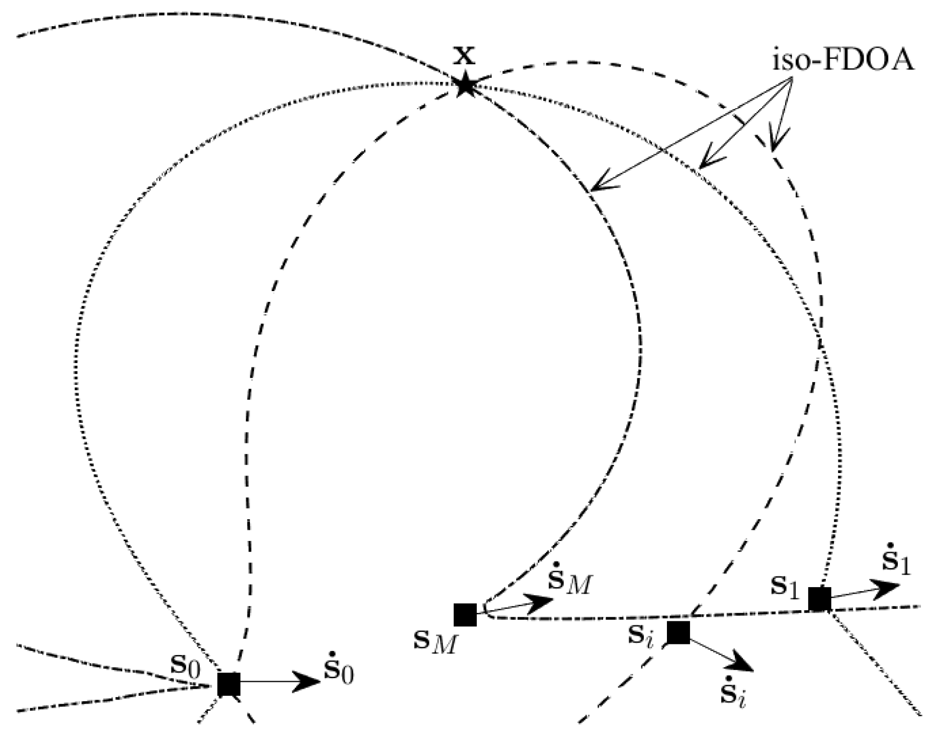
As depicted in Figure 2, let $\{{\mathbf{p}}_{11}^g,{\mathbf{p}}_{12}^g\}$ be two neighboring points on the $(z_1+3{\widehat{\sigma }}_f)$ iso-FDOA curve, and let $\{{\mathbf{p}}_{21}^g,{\mathbf{p}}_{22}^g\}$ be another two neighboring points on the $(z_1-3{\widehat{\sigma }}_f)$ iso-FDOA curve. The region circumscribed by these four points will be covered by the g-th Gaussian component. The center of the region determines the mean of the g-th Gaussian component ${\overline{\mathbf{x}}}_{1|1}^g$, the weight of the Gaussian component ${\overline{\omega }}_{1|1}^g$ is proportional to the area of this region, and the covariance of the Gaussian component ${\overline{\mathbf{P}}}_{1|1}^g$ depends on the orientation of the enclosing ellipse. Mathematically, we have [43]

$$\begin{array}{cc}\hfill & {\overline{\mathbf{x}}}_{1|1}^g={\displaystyle \frac{1}{2}}({\mathbf{y}}_1^g+{\mathbf{y}}_2^g),\hfill \end{array}$$

(35a)

$$\begin{array}{cc}\hfill & {\overline{\mathbf{P}}}_{1|1}^g=[{\mathbf{e}}_1^g,{\mathbf{e}}_2^g]\left[\begin{array}{cc}{d}_1^2\left(g\right)& 0\\ 0& d_2^2\left(g\right)\end{array}\right]\left[\begin{array}{c}{\left({\mathbf{e}}_1^g\right)}^T\\ {\left({\mathbf{e}}_2^g\right)}^T\end{array}\right],\hfill \end{array}$$

(35b)

$$\begin{array}{cc}\hfill & {\overline{\omega }}_{1|1}^g\propto \sqrt{\left|{\overline{\mathbf{P}}}_{1|1}^g\right|},\hfill \end{array}$$

(35c)

where ${\mathbf{y}}_1^g=({\mathbf{p}}_{11}^g+{\mathbf{p}}_{21}^g)/2$, ${\mathbf{y}}_2^g=({\mathbf{p}}_{12}^g+{\mathbf{p}}_{22}^g)/2$, ${\mathbf{e}}_1^g=({\mathbf{y}}_2^g-{\mathbf{y}}_1^g)/\parallel {\mathbf{y}}_2^g-{\mathbf{y}}_1^g\parallel$, ${\mathbf{e}}_2^g$ is a unit vector orthogonal to ${\mathbf{e}}_1^g$ such that ${\left({\mathbf{e}}_2^g\right)}^T{\mathbf{e}}_1^g=0$ and $\parallel {\mathbf{e}}_2^g\parallel =1$. The lengths of the semi-major and semi-minor axes are given by

$$\begin{array}{cc}\hfill & d_1\left(g\right)={\displaystyle \frac{1}{2}}{({\mathbf{y}}_2^g-{\mathbf{y}}_1^g)}^T{\mathbf{e}}_1^g,\hfill \end{array}$$

(36a)

$$\begin{array}{cc}\hfill & d_2\left(g\right)={\displaystyle \frac{1}{2}}{({\mathbf{y}}_3^g-{\mathbf{y}}_4^g)}^T{\mathbf{e}}_2^g,\hfill \end{array}$$

(36b)

where ${\mathbf{y}}_3^g=({\mathbf{p}}_{11}^g+{\mathbf{p}}_{12}^g)/2$ and ${\mathbf{y}}_4^g=({\mathbf{p}}_{21}^g+{\mathbf{p}}_{22}^g)/2$.

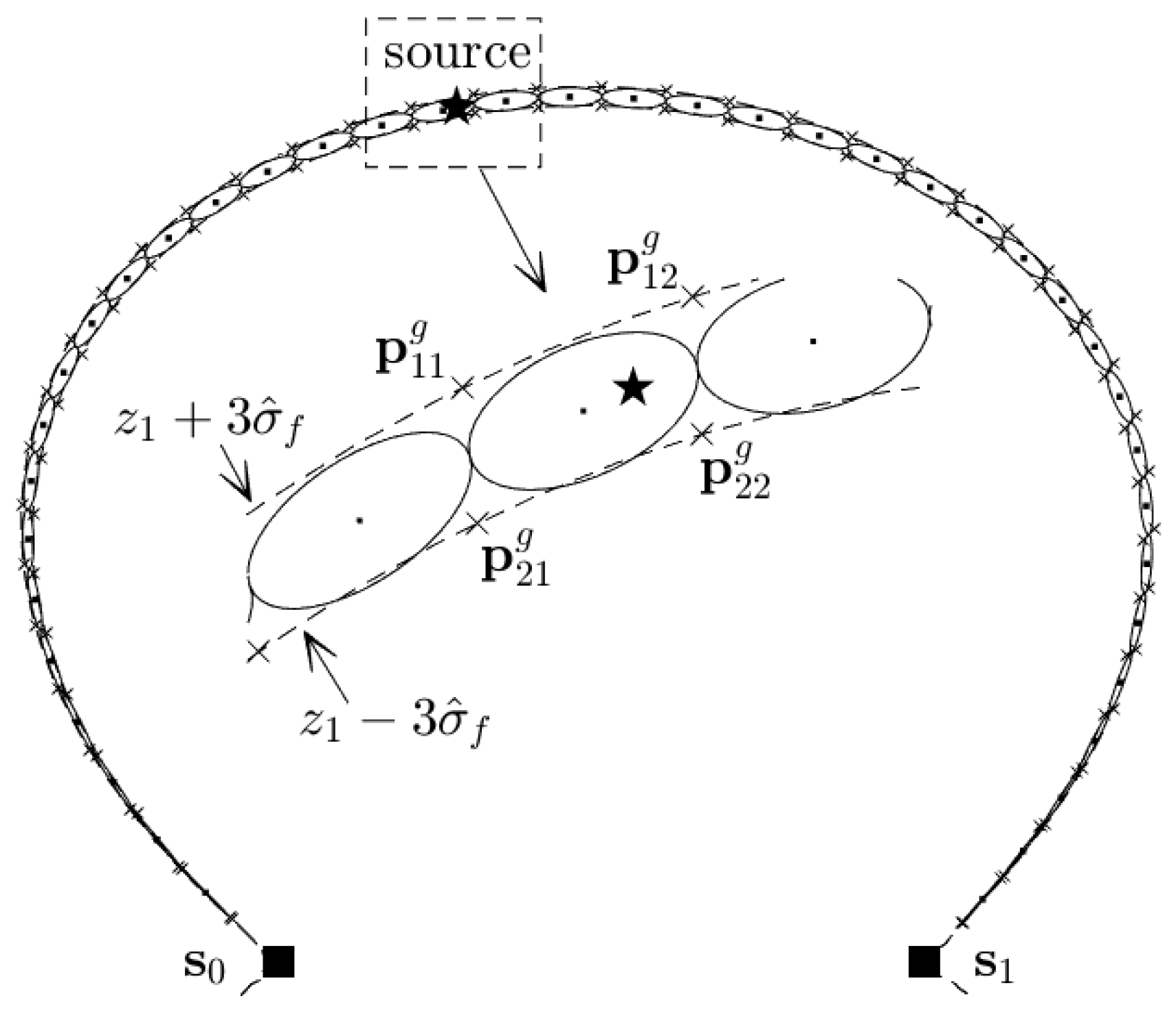
To obtain $\{{\mathbf{p}}_{11}^g,{\mathbf{p}}_{12}^g\}$ and $\{{\mathbf{p}}_{21}^g,{\mathbf{p}}_{22}^g\}$, we resort to the joint TDOA-FDOA localization method for a scenario with two sensors (in our case, ${\mathbf{s}}_0$ and ${\mathbf{s}}_1$) from [48]. Specifically, we first produce $(N_g+1)$ linearly spaced virtual TDOAs ranging from $-{\displaystyle \frac{1}{c}}\parallel {\mathbf{s}}_1-{\mathbf{s}}_0\parallel$ to ${\displaystyle \frac{1}{c}}\parallel {\mathbf{s}}_1-{\mathbf{s}}_0\parallel$ such that we obtain a set of virtual TDOAs, $\{\Delta t_1,\Delta t_2,\dots ,\Delta t_{N_g+1}\}$, where $\Delta t_g<\Delta t_{g+1}$. Then, as shown in Figure 3, the iso-TDOA curves represent the loci of constant TDOA, and ${\mathbf{p}}_{11}^g$ (or ${\mathbf{p}}_{21}^g$) is then found using joint TDOA-FDOA localization [48], with a TDOA of $\Delta t_g$ and an FDOA of $z_1+3{\widehat{\sigma }}_f$ (or $z_1-3{\widehat{\sigma }}_f$). However, ${\mathbf{p}}_{12}^g$ (or ${\mathbf{p}}_{22}^g$) is obtained using a TDOA of $\Delta t_{g+1}$ and an FDOA of $z_1+3{\widehat{\sigma }}_f$ (or $z_1-3{\widehat{\sigma }}_f$).

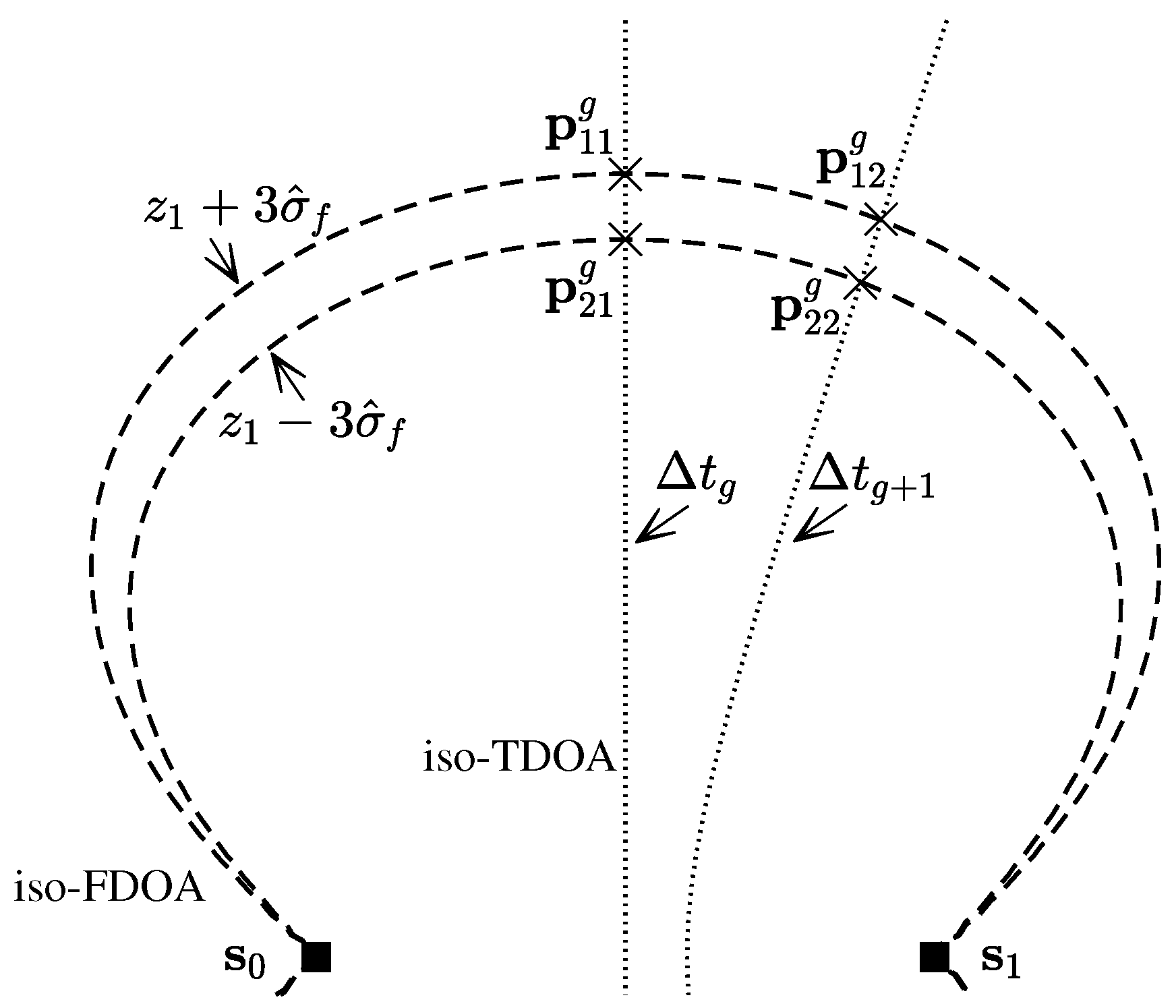
At the end of this section, we summarize the proposed GDM algorithm for FDOA-only localization in Algorithm 1.

Algorithm 1: The GDM Localization Algorithm

5. Algorithm Performance Analysis

5.1. Computational Complexity Analysis

The proposed GDM algorithm has three steps: GMM-based initialization, KF-1, and KF-2. Initially, $N_g$ Gaussian components are generated by solving the $2(N_g+1)$ intersections between the iso-FDOA and iso-TDOA curves using the algebraic localization method in [48]. Since all matrix operations involve computations of fixed dimensionality, this stage needs $\mathcal{O}\left(N_g\right)$ computational complexity. In the KF-1 step, the eigenvalue decomposition of the $M\times M$ measurement noise covariance matrix $\mathbf{R}$ is performed to derive the diagonal covariance in (11), requiring $21M^3$ multiplications and $10M^3$ additions. Subsequently, each Gaussian component undergoes $M-1$ CKF updates, incurring a complexity of $\mathcal{O}\left(N_{g}M\right)$. The total complexity of this stage is therefore $\mathcal{O}(M^3+N_{g}M)$. In the KF-2 step, computing the covariance matrix in (24) involves three matrix inversions, which has in total $2M^3$ multiplications and $2M^3+M^2$ additions. The final CKF update requires $21M^3+11M^2+39M+16$ multiplications and $10M^3+11M^2+28M+11$ additions, leading to a complexity of $\mathcal{O}\left(N_g{M}^3\right)$ for this stage. Collectively, the GDM algorithm induces an overall computational complexity of $\mathcal{O}\left(N_g{M}^3\right)$.

5.2. CRLB of the Algorithm

The CRLB is fundamental in estimation theory because it provides the minimum estimation error that any unbiased estimator can achieve [49]. Based on the Gaussian assumption of the measurement noise, the FDOA measurement likelihood function is given in (8b). From (4), the CRLB for source localization is given by

$$\mathrm{CRLB}\left(\mathbf{x}\right)={\left[{\left({\displaystyle \frac{\partial \mathbf{h}\left(\mathbf{x}\right)}{\partial \mathbf{x}}}\right)}^T{\mathbf{R}}^{-1}\left({\displaystyle \frac{\partial \mathbf{h}\left(\mathbf{x}\right)}{\partial \mathbf{x}}}\right)\right]}^{-1},$$

(37)

where

$${\displaystyle \frac{\partial \mathbf{h}\left(\mathbf{x}\right)}{\partial \mathbf{x}}}={\displaystyle \frac{f_c}{c}}·\left[\begin{array}{c}-\left({\mathbf{r}}_0^T{\dot{\mathbf{s}}}_0\right){\mathbf{r}}_0^T/r_0+{\dot{\mathbf{s}}}_0^T/r_0+\left({\mathbf{r}}_1^T{\dot{\mathbf{s}}}_1\right){\mathbf{r}}_1^T/r_1-{\dot{\mathbf{s}}}_1^T/r_1\\ -\left({\mathbf{r}}_0^T{\dot{\mathbf{s}}}_0\right){\mathbf{r}}_0^T/r_0+{\dot{\mathbf{s}}}_0^T/r_0+\left({\mathbf{r}}_2^T{\dot{\mathbf{s}}}_2\right){\mathbf{r}}_2^T/r_2-{\dot{\mathbf{s}}}_2^T/r_2\\ ⋮\\ -\left({\mathbf{r}}_0^T{\dot{\mathbf{s}}}_0\right){\mathbf{r}}_0^T/r_0+{\dot{\mathbf{s}}}_0^T/r_0+\left({\mathbf{r}}_M^T{\dot{\mathbf{s}}}_M\right){\mathbf{r}}_M^T/r_M-{\dot{\mathbf{s}}}_M^T/r_M\end{array}\right],$$

(38)

and the definitions of ${\mathbf{r}}_i$ and $r_i$ can be found in (2). Here, we omitted the reliance of ${\mathbf{r}}_i$ and $r_i$ on the source position $\mathbf{x}$ for notational simplicity.

6. Simulations

To validate the theoretical development and assess the performance of the proposed Bayesian FDOA-only localization algorithm, we conduct extensive Monte Carlo simulations. These experiments benchmark our algorithm against two established techniques, namely, the FDOAR method [36] and the iterative GN approach [37]. Furthermore, to demonstrate the superiority of the proposed FDOA-only method over the TSWLS [30] algorithm, which is based on jointly exploiting the TDOA and FDOA measurements for positioning, two TDOA noise levels are considered: (i) a low TDOA noise level, where ${\sigma }_t=0.35{\sigma }_f$, and (ii) a high TDOA noise level, with ${\sigma }_t=300{\sigma }_f$. To evaluate the impact of the initial solution quality on the final localization result of the iterative GN algorithm, the initial solutions are centered at the true source position but subject to an additive zero-mean Gaussian error whose covariance is equal to $20\mathrm{CRLB}\left(\mathbf{x}\right)$. The number of iterations for the GN is set to 3. Meanwhile, to investigate the effect of including the KF-2 step in the GDM algorithm on the source positioning accuracy, the simulation results relying solely on the KF-1 step are included for comparison.

A stationary target, positioned at $\mathbf{x}={[3,10]}^T$ km, is considered in this section. It transmits signals with a carrier frequency of $f_c=3$ GHz. The speed of signal propagation is $c=3\times {10}^8$ m/s.

Table 1. Positions and velocities of the observers.

Observer No.	Position (m)	Velocity (m/s)
1	${\mathbf{s}}_1={[0,0]}^T$	${\dot{\mathbf{s}}}_1={[100,0]}^T$
2	${\mathbf{s}}_2={[2000,0]}^T$	${\dot{\mathbf{s}}}_2={[110,4]}^T$
3	${\mathbf{s}}_3={[1500,1000]}^T$	${\dot{\mathbf{s}}}_3={[138,24]}^T$
4	${\mathbf{s}}_4={[-500,500]}^T$	${\dot{\mathbf{s}}}_4={[75,27]}^T$
5	${\mathbf{s}}_5={[3000,5000]}^T$	${\dot{\mathbf{s}}}_5={[142,-5]}^T$
6	${\mathbf{s}}_6={[-1000,1000]}^T$	${\dot{\mathbf{s}}}_6={[76,-39]}^T$
7	${\mathbf{s}}_7={[-500,6000]}^T$	${\dot{\mathbf{s}}}_7={[92,43]}^T$
8	${\mathbf{s}}_8={[1500,3000]}^T$	${\dot{\mathbf{s}}}_8={[82,9]}^T$
9	${\mathbf{s}}_9={[1000,-1000]}^T$	${\dot{\mathbf{s}}}_9={[117,-27]}^T$

summarizes the spatial coordinates and velocities of the observers. The number of Gaussian components in the GMM model is $N_g=20$, and the scaling factor in (26a) is $\alpha ={10}^{-6}$. A total number of L = 10,000 Monte Carlo runs are conducted. The performance of the algorithm is quantified using the positioning root mean square error (RMSE), defined to be

$$\mathrm{RMSE}\left(\mathbf{x}\right)=\sqrt{{\displaystyle \frac{1}{L}}{\sum }_{l=1}^L{\parallel \mathbf{x}-{\widehat{\mathbf{x}}}_l\parallel }^2},$$

(39)

where ${\widehat{\mathbf{x}}}_l$ denotes the target position estimate in the l-th ensemble run.

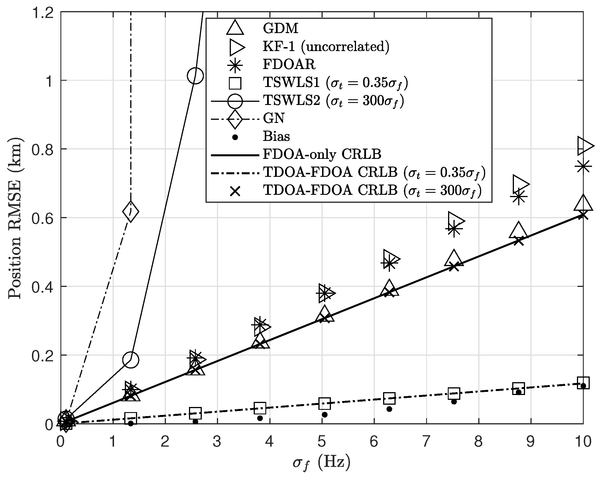
As shown in Figure 4, we compare the localization performance of the proposed GDM against that of several benchmark algorithms under varying measurement noise levels. To demonstrate the advantages of our proposed algorithm over the FDOAR algorithm in the over-determined scenarios, this simulation uses the first four observation stations listed in Table 1. The measurement noise standard deviation varies from 0.1 to 10 Hz. The results highlight the robustness of our approach across the considered FDOA noise levels. The figure also shows that the GDM attains performance close to the CRLB at low and moderate FDOA noise levels. The estimation bias of the proposed GDM algorithm is small compared to the RMSE.

Furthermore, in Figure 4, we can observe that the positioning performance of using the KF-1 step only is suboptimal because it fails to account for the correlation between the FDOA measurements. The FDOAR algorithm exhibits degraded localization performance as the measurement noise increases. However, it cannot achieve the CRLB, not even under low-noise conditions. This is because it does not utilize all the available FDOAs for positioning.

The CRLBs of the joint TDOA-FDOA localization at different levels of TDOA noise are included in Figure 4 for comparison. It can be seen that, under low TDOA noise (${\sigma }_t=0.35{\sigma }_f$), the RMSE of the TSWLS method aligns with the CRLB, signifying its optimal performance in the presence of low noise. Conversely, in the presence of significant TDOA noise (${\sigma }_t=300{\sigma }_f$), the CRLBs for the FDOA-only and TDOA-FDOA positioning become very close to each other, as expected. However, the performance of the TSWLS method evidently deviates from the CRLB. This reveals that the TSWLS method is very sensitive to the increased TDOA noise level. However, the GN method diverges, even at low noise levels, mainly because of a relatively large initialization error. This highlights the significant impact of initial value quality on the performance of the iterative GN method.

The average execution times of various localization methods are summarized in

Table 2. Average computation times of different methods.

Method	Average Time (ms)
GDM	2.62
KF-1 (uncorrelated)	0.81
FDOAR	2.82
GN	0.108
TSWLS1	0.11
TSWLS2	0.063

. The experiment was performed on an Intel Core i9-13900H processor, with a clock frequency of 2.60 GHz. As shown in Table 2, the proposed GDM algorithm exhibits longer computation times than existing methods, though it maintains practical feasibility for real-time applications. The increased computational cost of the GDM arises primarily from its GMM implementation, which necessitates updating all components whenever a new set of FDOAs is obtained. While acceleration techniques for GMMs have been thoroughly studied [50,51,52], our primary contribution focuses on introducing the GDM framework for FDOA-only localization rather than computational optimization.

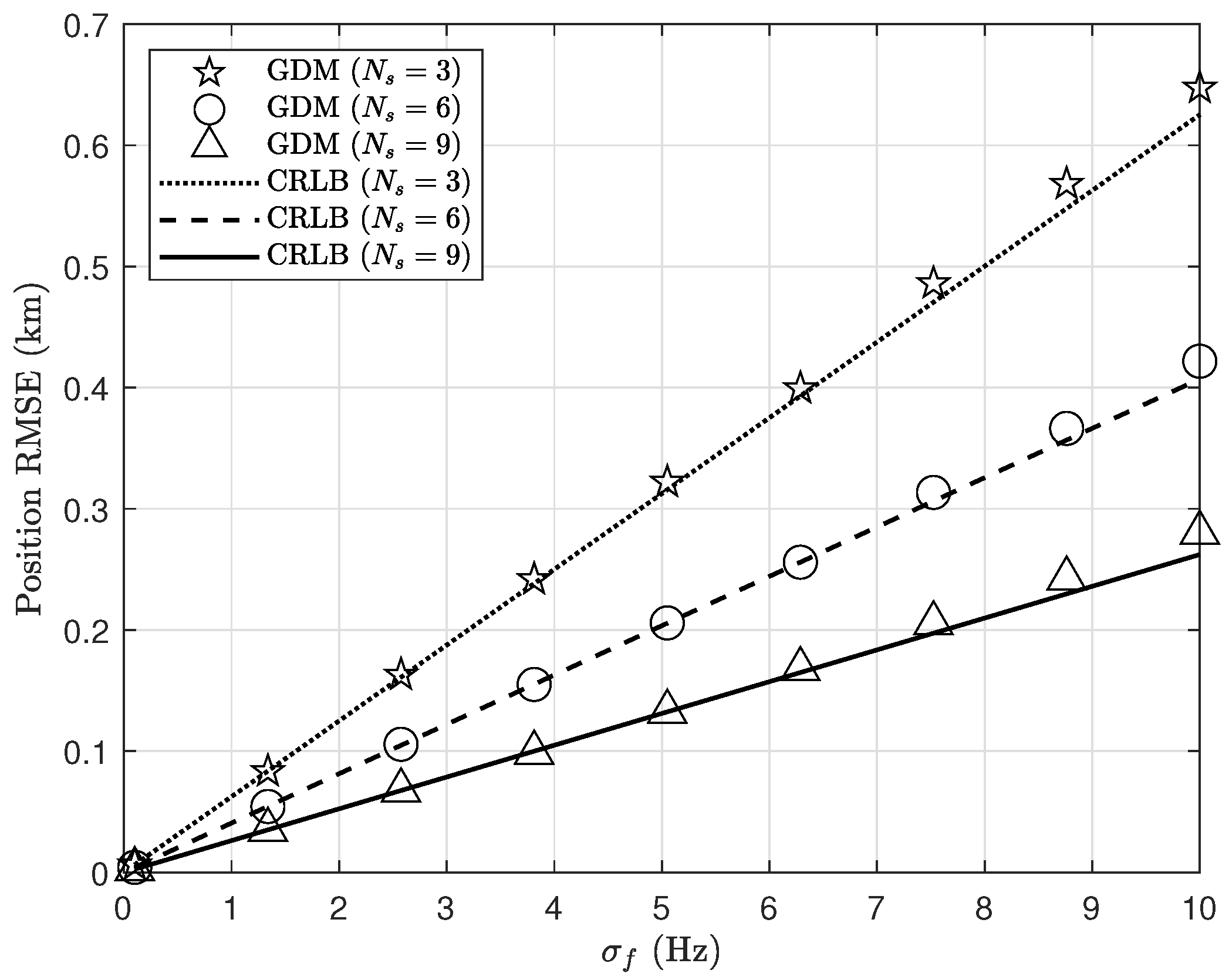
In Figure 5, we evaluate the performance of the proposed GDM under varying numbers of observers, denoted as $N_s$ ($N_s=3,6,9$). The positions and velocities of the observers are detailed in Table 1. Figure 5 demonstrates that the GDM achieves the CRLB accuracy under varying numbers of observers. This scalability is crucial for practical applications where the number of available observers may vary.

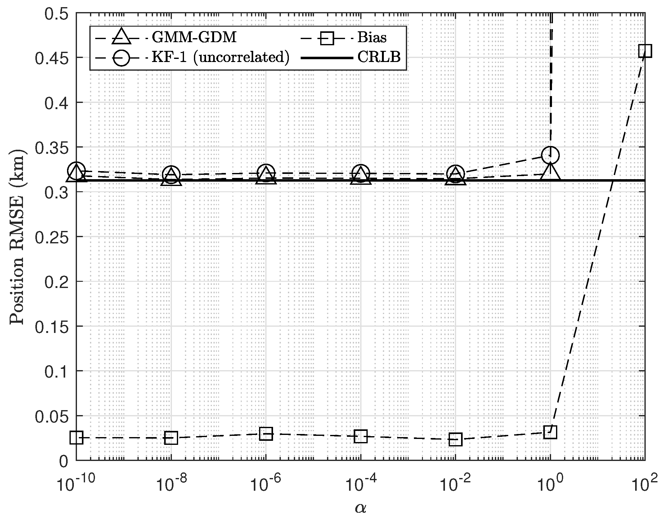
The scaling factor $\alpha$ in (26b) ensures the positive definiteness of ${\mathbf{\Sigma }}^{-1}$. In Figure 6, the estimation performance of the developed algorithm is evaluated under different scaling factor values ($\alpha ={10}^{-10},{10}^{-8},{10}^{-6},{10}^{-4},{10}^{-2},{10}^0$ and ${10}^2$), with the standard deviation of the FDOA measurement noise fixed at 5 Hz. The proposed GDM algorithm achieves the CRLB even when $\alpha$ is as small as ${10}^{-10}$, demonstrating the numerical stability of the GDM. However, when $\alpha$ becomes too large, the diagonal elements of $\mathbf{D}$ also increase, causing the localization results of KF-1 to greatly deteriorate, eventually leading to deviation from the CRLB. This suggests that $\alpha$ should be chosen from a reasonable range.

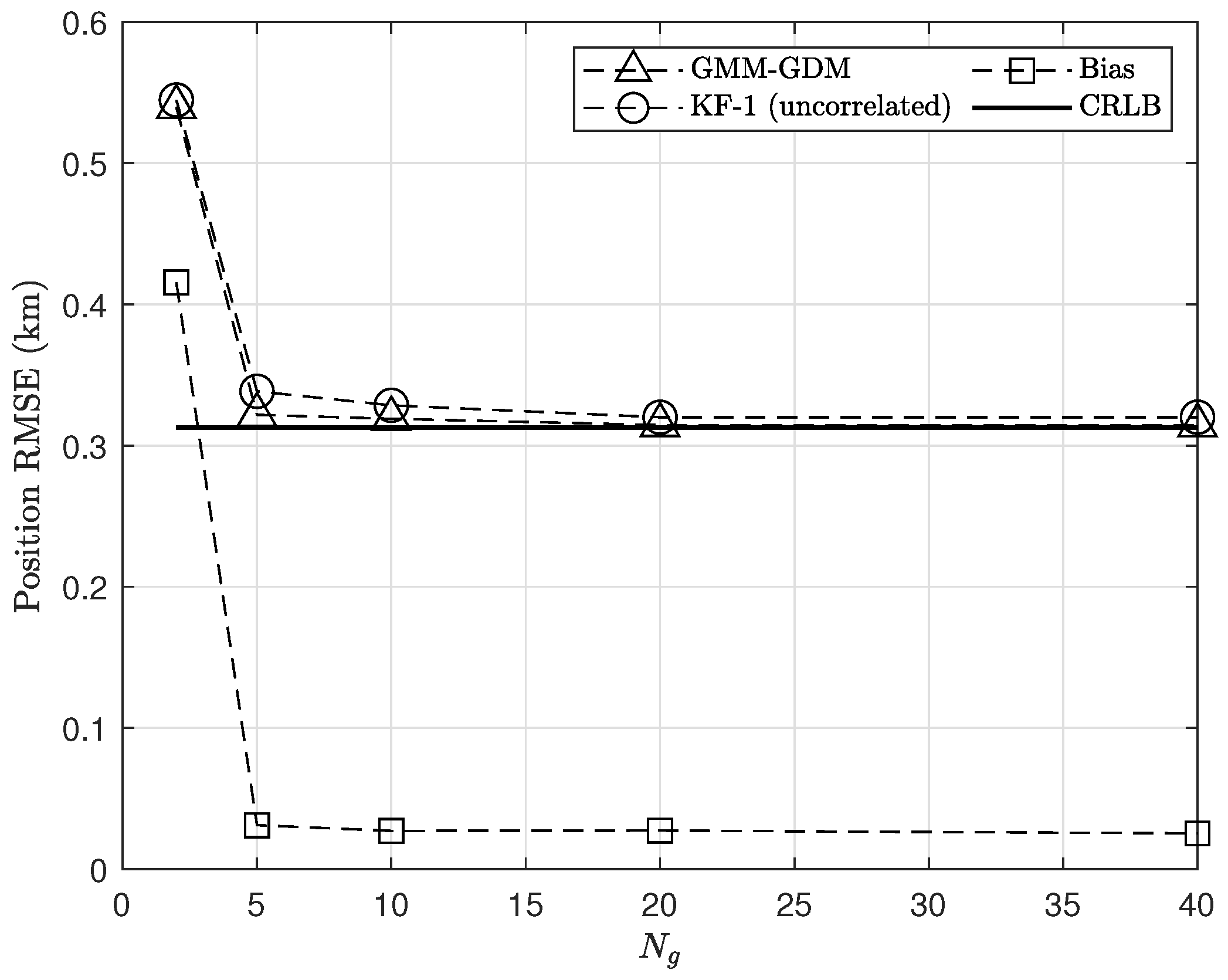
Using a larger number of initial Gaussian components during the GMM initialization phase should better approximate the true but unknown source position prior. However, an excessive number of components increases the computational burden. In Figure 7, the localization performance of the proposed GDM is evaluated under different numbers of Gaussian components $N_g$ (specifically at 2, 5, 10, 20, and 40), with the FDOA measurement noise again fixed at ${\sigma }_f=5$ Hz. The results indicate that the localization accuracy of the GDM improves with an increasing number of Gaussian components. But it already achieves near CRLB accuracy when $N_g=5$. This demonstrates the algorithm’s ability to deliver satisfactory localization precision without incurring excessive computational demands. Furthermore, this study reveals that, during the update of the source position posterior using the FDOA measurements sequentially, the weights of the Gaussian components far from the target’s actual position would significantly decrease. Consequently, by pruning the Gaussian components with small weights, computational efficiency can be further improved. This type of operation has been described in existing work such as [53] and will not be elaborated here.

7. Conclusions

This paper addresses the challenge of single stationary target localization exclusively using FDOA measurements. The inherent strong nonlinearity in FDOA measurement models presents substantial challenges for numerical solution development and implementation. To overcome these limitations, we employ the GMM for a probabilistic representation of the initial FDOA measurement, constructing a high-confidence spatial probability region where the target resides. The differential framework utilizing a common reference station induces intrinsic measurement noise correlations, necessitating specialized sequential updating mechanisms for subsequent FDOA measurements.

The core contribution of this work is the GDM, a novel Bayesian localization framework featuring a dual-phase Kalman implementation that systematically exploits measurement noise correlations. The first phase (KF-1) employs sequential Bayesian filtering with GMM-derived priors to generate coarse estimates under measurement noise independence assumptions. Subsequent refinement in the second phase (KF-2) incorporates explicit correlation modeling through likelihood ratio correction, effectively compensating for information loss during the initial decoupling process and yielding optimized posterior probability distributions.

Comprehensive numerical simulations validate three principal advantages of our approach: (1) capability for precise localization with minimal infrastructure requirements (as few as three stations in a 2D scenario), (2) enhanced robustness against significant measurement noise levels, and (3) computational efficiency suitable for real-time implementation. The methodology’s generalizability is demonstrated by its applicability beyond FDOA systems to broader nonlinear estimation problems, particularly those involving correlated measurement architectures.