Landslide Segmentation in High-Resolution Remote Sensing Images: The Van–UPerAttnSeg Framework with Multi-Scale Feature Enhancement

Abstract

Among geological disasters, landslides are a common and extremely destructive disaster. Their rapid identification is crucial for disaster analysis and response. However, traditional methods of landslide recognition mainly rely on visual interpretation and manual recognition of remote sensing images, which are time-consuming and susceptible to subjective factors, thereby limiting the accuracy and efficiency of recognition. To overcome these limitations, for high-resolution remote sensing images, this method first uses online equalization sampling and enhancement strategy to sample high-resolution remote sensing images to ensure data balance and diversity. Then, it adopts an encoder–decoder structure, where the encoder is a visual attention network (Van) that focuses on extracting discriminative features of different scales from landslide images. The decoder consists of a pyramid pooling module (PPM) and feature pyramid network (FPN), combined with a convolutional block attention module (CBAM) module. Through this structure, the model can effectively integrate features of different scales, achieving precise positioning and recognition of landslide areas. In addition, this study introduces a sliding window algorithm based on Gaussian fusion as a post-processing method, which optimizes the prediction of landslide edge in high-resolution remote sensing images and ensures the context reasoning ability of the model. In the validation set, this method achieved a significant landslide recognition effect with a Dice score of 84.75%, demonstrating high accuracy and efficiency. This result demonstrates the importance and effectiveness of the research method in improving the accuracy and efficiency of landslide recognition, providing strong technical support for analysis and response to geological disasters.

1. Introduction

As a common geological disaster, a landslide poses a serious threat to the safety of human life and property. Not only does it cause huge direct economic losses, but it can also cause long-term casualties and environmental damage [1]. A landslide occurs when soil or rock formations on a slope move downward, either as a cohesive mass or in fragments, along a particular weak surface or zone. This movement is triggered by various natural factors, including river erosion, groundwater activity, rainwater saturation, and earthquakes, as well as human activities such as slope excavation and construction [2]. The occurrence of landslides is highly uncertain, involving a variety of factors such as lithology, faults, altitude, and slope, which makes it extremely difficult to predict the exact time and location of the landslides [3]. Therefore, post-disaster assessment of landslides is particularly important, as it not only reveals the specific damage caused by landslides but also provides a scientific basis for the formulation of post-disaster response strategies and emergency rescue plans [4]. Through post-disaster evaluation, we can learn more about the scope, extent, and affected area of landslide disasters, which provides an important reference for post-disaster reconstruction and recovery [5]. At the same time, the assessment results can also provide guidance and support for future disaster prevention efforts, helping us to better understand and respond to landslide disasters. Therefore, post-disaster landslide evaluation is a major focus of geological disaster research at present.

With the development of remote sensing technology, landslide recognition technology is becoming more and more accurate, and identifying the landslide area contained in remote sensing images plays an important role in post-disaster assessment. The traditional method is often to recognize the landslide area of the remote sensing image employing manual visual judgment [6]. For example, in 2009, Tsai, Fand, et al. [7] used multi-temporal satellite images to conduct a post-disaster assessment of landslides in southern Taiwan by comparing them with other geospatial data; they accurately identified the impact range of landslides. In 2010, F. Fiorucci et al. [8] conducted a visual analysis of the landslide in the Apennines Mountains through aerial orthophoto and satellite images, and finally determined the impact range of the landslide and analyzed the causes of the landslide. Although the visual interpretation method can accurately identify the extent of the impact of the landslide, the uncertainty caused by manual interpretation is very high.

With recent advancements in computer technology, many methods have emerged in this regard, mainly in machine learning and deep learning, and common machine learning algorithms include logistic regression [9], support vector machines [10], random forests [11]. Since 2005, Tolga Can et al. [12] have been using logistic regression analysis to analyze the factors that cause landslides, and the frequency of use is increasing. In 2013, Biswajeet Pradhan et al. compared decision trees, support vector machines, and adaptive neural fuzzy inference systems to evaluate landslides, and concluded that the sensitivity of the model to the landslide domain on the map is reliable. In 2017, Wei Chen et al. [13] compared machine learning methods such as the logistic model tree [14], random forest, and categorical regression tree (CART) model, and proved the reliability of their methods in landslide sensitivity spatial prediction.

The development of computers has driven the development of machine learning, and a range of deep learning methods have emerged. Unlike traditional machine learning approaches, deep learning is a highly effective, supervised method [15] that is both time-efficient and cost-efficient. It encompasses a wide range of architectures and topologies, making it suitable for addressing numerous complex problems. Deep learning is considered to be the best option for discovering complex architectures in high-dimensional data by using backpropagation algorithms.

With the continuous development of deep learning, many algorithm models have emerged, such as AlexNet [16], RCNN [17], Fast RCNN [18], YOLO [19], SSD [20], and an increasing number of scholars are applying deep learning across various fields, including remote sensing. In deep learning applications for remote sensing, scholars mainly focus on detection tasks and segmentation tasks. The detection task is a type of recognition method that can identify the slip area, while the segmentation task is a pixel-based recognition method that can classify each pixel of the picture to better evaluate the landslide area.

In terms of landslide detection, M. I. Sameen et al. [21] proposed integrating the residual network into the landslide detection model and fusing spectral bands with terrain data, which improved the accuracy of landslide detection to an accuracy rate of 81.6%. Cheng et al. [22] proposed an improved landslide detection model, YOLO-SA based on YOLOv4 [23], which reduced the parameters of the model and added an attention mechanism to improve the accuracy of the model, with an accuracy rate of 94.08%, using Qiaojia County and Ludian County of Yunnan Province in China as the study areas. Jian Xiaoting et al. [24] used the Faster R-CNN model for landslide detection; the AP obtained was 92.42%. Tao Wang et al. [25] improved the YOLOv5 model, added adaptive spatial feature fusion, and introduced the convolutional block attention mechanism (CBAM) under its basic framework, and the overall performance of the model increased by 1.64%.TAN. Other researchers [26] fused the digital elevation model (DEM) with the landslide recognition model and finally improved the IoU and F1 by 9.3% and 6.8%, respectively.

Remote sensing algorithms can accurately identify landslide locations. On the other hand, remote sensing landslide segmentation tasks can precisely demarcate the boundaries of landslides and determine the proportion of landslide areas within the overall image. Consequently, remote sensing landslide segmentation algorithms are effective tools for studying changes in landslide areas and for calculating landslide extents. For common segmentation models, such as U-Net [27], PSNet [28], DeepLabv3 [29], and SegNet [30], many scholars have studied the segmentation task in the field of landslide segmentation. Soares et al. [31] utilized DEM (digital elevation model) data as the basis for training and employed the U-Net model to automatically identify and segment landslide areas in Novo Fribourg City, which is situated in the mountainous region of Rio de Janeiro, southeastern Brazil. The model achieved F1 scores of 0.55 and 0.58 on two distinct test datasets. C Fang et al. [32] introduced a lightweight attention mechanism into the U-Net model to obtain an F1 score of 87.45%, and Zhun Li [33] adopted the MobileNetV2 structure of the backbone network of PSPNet to reduce network parameters, improve the network convergence speed, and improve the accuracy of object division. Du et al. [34] conducted a comparative analysis of six prevalent deep learning models for semantic segmentation tasks, utilizing a custom-built landslide dataset from the Yangtze River coastal region. The evaluation concluded with the GCN model, achieving an accuracy of 0.542, and the DeepLabv3 model achieved a mean intersection over union (mIoU) score of 0.740. Lu Yun [35] improved the performance of the Mask R-CNN by incorporating the CBAM attention mechanism and enhancing the feature pyramid network with bottom-up channels, resulting in an accuracy of 92.6%. This method ensures the comprehensive integration of semantic features across all channels.

Although many scholars have made many remarkable achievements in the task of landslide segmentation, there are still some problems to be solved in this field.

• Unbalanced landslide data: Landslides vary in size and shape, from small local landslides to large regional landslides. Landslides are unevenly distributed on remote sensing images, and the balance of data has a great impact on the model’s recognition ability. Different types of landslides appear significantly different on images, from small shallow landslides to large deep landslides, and their characteristics and influencing factors are different. In particular, the imbalance of positive and negative samples will cause the model to be biased toward categories with fewer samples, affecting the model’s recognition ability.
• Model recognition capability: The terrain in mountainous canyon areas is complex and the vegetation coverage varies greatly. It is difficult to distinguish landslide areas in remote sensing images. In some areas, the vegetation coverage varies greatly, resulting in discontinuity, while some areas with human activities are not landslides, which increases the difficulty of model recognition.
• Post-processing: Most researchers crop high-resolution images and then use these cropped images to identify landslides, a method that lacks engineering capabilities.

Given this, this paper proposes a Van–UPerAttnSeg cross-fusion model, which comprehensively optimizes the segmentation task from three key dimensions. First, the data-balancing algorithm is designed, second, the model network is optimized, and third, the post-processing process is improved. Compared with other models, the Van–UPerAttnSeg model showed better data. It is worth noting that all the evaluation indicators in this paper are calculated directly on the original diagram, which ensures that the research results are not only theoretical but also have high engineering application value. The key contributions of this article are as follows.

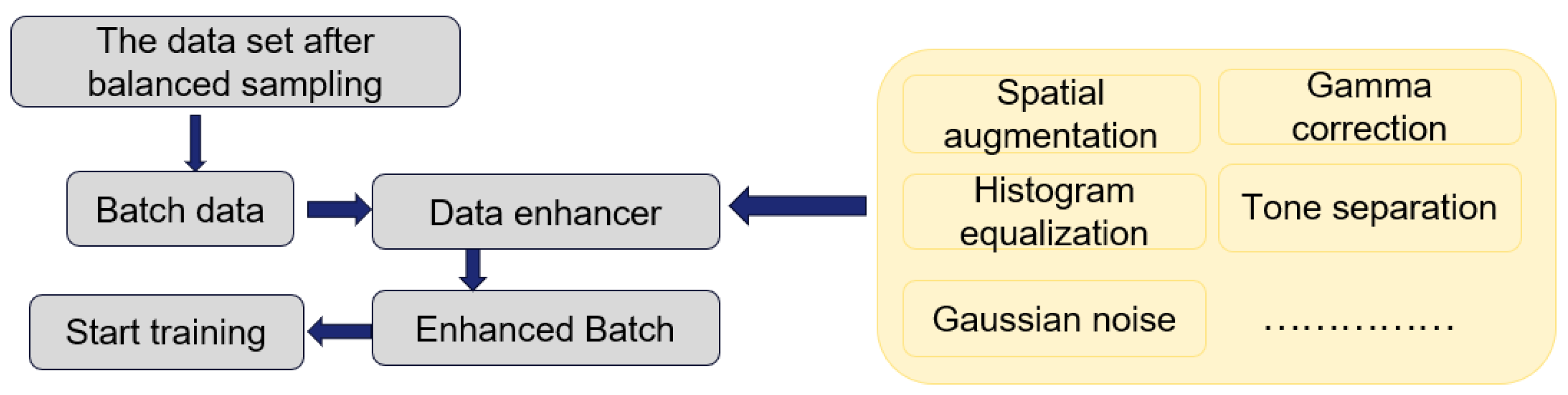
• This paper designs an efficient data enhancement algorithm to solve the data problem through online balanced sampling and online data enhancement. Through this method, the dataset reaches a relatively balanced state between categories, reduces the deviation in the segmentation task, and increases the robustness of the model through online enhancement.
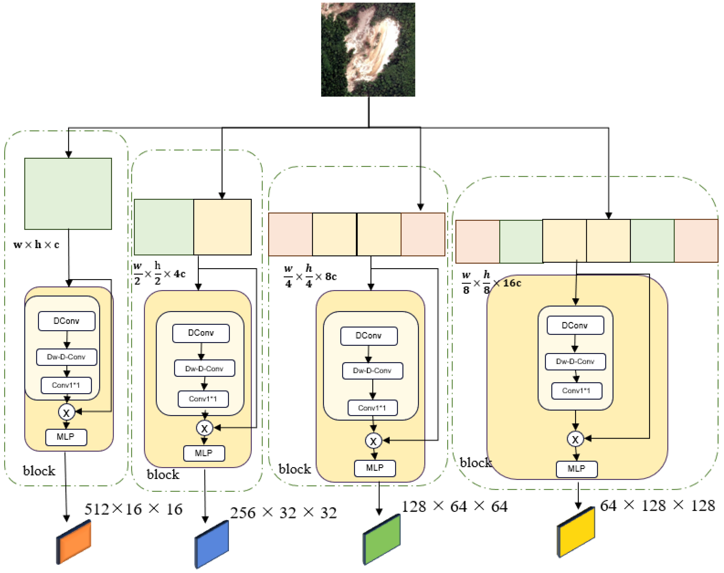
• This paper proposes a new landslide recognition model, Van–UPerAttnSeg. An encoder–decoder structure is used to identify landslides. The Van network is introduced in the encoder to extract multi-level features of landslides. In the decoder, a pyramid structure is introduced to fuse multi-scale features, and the fused features are further processed with the help of the CBAM module.
• In the post-processing stage, this paper proposes a sliding window-based Gaussian blur algorithm that can address image boundary issues and significantly reduce the requirements for computing devices. Through this method, the model can generate high-quality segmentation results more efficiently when processing high-resolution images, further enhancing the model’s practicality and engineering.

2. Methods

2.1. Data Augmentation Methods

The ability of a neural network to learn effectively is significantly influenced by the number of samples and the balance between positive and negative samples [36], while in the image segmentation task, its learning ability is more affected by the pixel distribution. To tackle this issue, this paper suggests a method for equalizing sampling, which can achieve the balance of the dataset at the pixel level as much as possible. The images sampled by this method can make the dataset achieve a more balanced state among the categories. After the dataset is balanced, we further use online data augmentation techniques to improve the performance of the model. The specific steps are as follows:

• First, the pixels in the dataset are calculated as shown in

  Table 1. Distribution statistics of non-landslide pixels (1) and non-landslide pixels (0).

  	Number	Ration (%)	Total
  0	447,075,372	79.03	565,730,464
  1	118,655,092	20.97

  . The dataset will then be divided in a balanced manner according to the statistical results, ensuring that the proportions of pixels in the validation set and the training set are similar to those in the overall dataset. The division of the datasets is detailed in

  Table 2. Division of the dataset by pixel percentage.

  	Number	Ration (%)	Total
  Train	79	73.9	107
  valid	28	26.1

  .

• After evenly dividing the dataset, this paper proposes a data-sampling method for balanced sampling and online enhancement [37] of the sampled tiles for the training set. Image online augmentation is the practice of augmenting data prior to each training iteration. This technique helps to increase the size of the dataset and enhance the model’s ability to generalize. The core procedures are as follows:

  –

  We generate a series of coordinate anchor points on the image to achieve uniform sampling of the image. Taking the 1024 × 1024 image used in this article as an example, we evenly distribute about 100 × 100 anchor points on the image. Based on the statistical pixel ratio, we sample according to the set tile size (512 × 512 in this article) to generate the corresponding tile.

  –

  When processing the tiles generated based on anchor points, we first calculate the ratio of each type of pixel in each tile. Specifically, we count the number of pixels in the landslide area and the non-landslide area in each tile. Then, we generate a probability value, x, for each tile based on the ratio of pixels in the landslide and non-landslide areas in the total dataset (1:4). In order to achieve a balanced partition of the tiles, we generate a random seed between 0 and 1. We select the value closest to the random seed and select the tile as the representative of the landslide area; we select another tile with a probability of (1 − x). In this way, we can ensure that the divided tiles are balanced in the distribution of landslide and non-landslide areas.

  –

  Setting the dataset length determines the number of tiles used in the training process. This number is determined based on the model training requirements and computing resource constraints. For example, if the model needs more data to improve generalization, the number of sampling points can be increased to generate more tiles.

• After obtaining the balanced dataset, we perform a series of online enhancement operations [38] on the image to improve the robustness of the model to different image conditions (see Figure 1). Online enhancement refers to the process of enhancing data before each iteration during the training process. This not only expands the dataset but also significantly improves the model’s generalization ability. The specific enhancement methods are as follows.

  –

  Spatial augmentation: Perform random flips on images, including horizontal and vertical flips, to increase the diversity of the data.

  –

  Gamma correction: Enhance the contrast and brightness of the image by randomly adjusting the gamma value, making the image more recognizable in different lighting conditions.

  –

  Histogram equalization: Improve the image’s overall contrast by adjusting the histogram distribution of the image to bring it closer to a uniform distribution.

  –

  Pixel value inversion and threshold adjustment: Invert or move pixel values in an image to a specific threshold to highlight key features in the image.

  –

  Hue, saturation, and brightness adjustments: Simulate different lighting and color conditions by randomly varying the hue, saturation, and brightness values of an image.

  –

  Tone separation: Tone separation is performed on an image to highlight the main color components in the image.

  –

  Add Gaussian noise: Add Gaussian noise to the image to enhance the robustness of the model to noise.

Figure 1. Online image enhancement, including adding filters, colors, space, etc.

Figure 1. Online image enhancement, including adding filters, colors, space, etc.

To understand the sampling technique proposed in this paper, the core steps are outlined as follows: First, we mark the corresponding anchor points on the image according to the preset step size. Next, we build a sampling frame (512 × 512 pixels) around each anchor point. Subsequently, the proportion of specific pixels in each sampling frame is calculated. On this basis, the tiles with similar proportions are selected through the overall pixel ratio. In the end, we have a well-balanced dataset and perform online enhancement processing on it to further improve the diversity and usefulness of the data. The specific steps are shown in Figure 2.

To visually demonstrate the advantages of balanced sampling, this paper compares it with the method of equal scaling combined with online enhancement. The scaling sampling strategy is as follows: First, the original image is scaled to the target resolution (512 × 512), and then a series of online enhancement operations is implemented on this basis. A detailed diagram of this process is shown in Figure 3.

2.2. Network Structure

The model proposed in this study adopts the classic encoder–decoder architecture. In the encoder section, the visual attention network (Van) network is used as the backbone network to fully exploit its advantages in feature extraction. In the decoder section, we introduce a pyramid structure to effectively combine the multi-dimensional features obtained from the encoder. To further optimize the feature fusion effect, we add a CBAM module to the fused features to enhance the model’s attention to key features. Finally, through this structural design, the model can achieve high-precision segmentation of the landslide image. The specific network structure is shown in Figure 4.

The encoder extracts multi-level features from a 512 × 512 image block. For the decoder, we use a pyramid structure to obtain and fuse features from different dimensions. By performing pooling and convolution operations on high-dimensional data, deep features are fused with shallow features. Finally, the feature dimensions are unified through the last convolution layer to obtain the predicted output. We will introduce each part of the model.

2.2.1. Image Encoder

The Van network is an improved Transform structure proposed by the Tsinghua University team in 2021 and proposed the large kernel attention (LKA) module. LKA absorbs the advantages of convolution and self-attention, including local structural information, long-range dependency, adaptability, etc., while also avoiding their shortcomings such as ignoring adaptability in the channel dimension. The comparison is shown in

Table 3. Comparison of convolution, self-attention, and LKA.

	Convolution	Self-Attention	LKA
Local perception	yes	no	yes
Long distance dependency	no	yes	yes
Spatial adaptability	no	yes	yes
Channel adaptability	no	no	yes

.

In this network structure, the PatchEmbed module uses convolution to process the input data and map it to the representation of the corresponding dimension. Subsequently, these feature representations are passed to the block module for further processing. The block module combines the large kernel attention mechanism (LKA) and the multi-layer perceptron (MLP), which can effectively capture feature information at different scales, giving full play to the advantages of the large kernel attention mechanism in long-distance dependency modeling, and combining the efficiency of MLP in local feature extraction. The output features, which are the 512-, 256-, 128-, and 64-dimensional features, represent the feature information under different fields of view, respectively. This multi-scale feature extraction method provides the model with more comprehensive contextual information, which not only enhances the generalization ability of the model and enables it to adapt to a variety of downstream tasks, but also improves the flexibility and superiority of the model when dealing with complex scenes. Its specific network structure is shown in Figure 5.

2.2.2. UPerAttn Decoder

In the decoder, the encoder extracts features of different field sizes, and to fuse these features more effectively, we use the pyramid pooling module (PPM) to perform pooling, upsampling, and convolution operations on the largest size features and fuse them with deeper level features. Subsequently, the feature pyramid network (FPN) is used to further integrate the feature maps of different scales to achieve the synergy of multi-scale information. To more effectively underscore the core characteristics, we introduce a CBAM module into the fused features, which is able to adaptively highlight important feature information. Finally, the prediction result with a size of 2 × 128 × 128 is generated by the convolution operation. The specific network structure is shown in Figure 6.

2.2.3. Loss Function

In deep learning, the loss function is a fundamental instrument between a model’s outputs and the ground truth. It calculates the prediction error for each sample and returns a scalar value to represent the loss of the entire training set. Based on this loss value, the parameters of the model are updated. Therefore, choosing the right loss function is critical for the training and performance of the model. Different loss functions behave differently under different data distributions and model structures, and the optimizer updates the model parameters according to the loss value to gradually reduce the loss and improve the accuracy of the model.

In the field of image segmentation, common loss functions include cross-entropy loss function, Dice loss function, etc. However, in order to better achieve the landslide segmentation task, this paper introduces a new loss function. Under the current training framework, this loss function not only has the best effect but also has the fastest convergence speed. Its main components are as follows:

LabelSmoothLimiteCrossEntropyLoss (LCE): LCE is an improved loss function proposed for the landslide segmentation task in this paper, which is extended and optimized based on the classical cross-entropy Loss. LCE first introduced the label smoothing technique to enhance the robustness of the model to uncertainty by softening the label distribution. In addition, LCE introduces the limited parameter to further control the behavior of the loss function, making it more suitable for the special needs of landslide segmentation tasks.

• Label smoothing: Label smoothing works by reducing the confidence level of the true label (i.e., reducing the true label from 1 to a smaller value, such as 0.96) and assigning a certain level of confidence to other categories (usually evenly distributing the remainder, such as 0.04/N, where N is the number of categories). Label smoothing helps to reduce the overfitting of the model, and encourages the model to maintain a certain uncertainty when predicting to enhance the model’s generalization ability instead of blindly predicting a single class. The formula is as follows:

  $$y_1=(1-s)·y_{ij}+{\displaystyle \frac{s}{C}}$$

  (1)

  where C is the number of categories, s is the smoothing parameter, $y_{ij}$ is the original label, and $y_1$ is the smoothed label.
• LimitCrossEntropyLoss: By introducing the limit parameter, the behavior of CrossEntropyLoss when the prediction probability is close to the extreme value (0 or 1) can be adjusted. A smaller limit value makes the loss curve steeper near the extreme predicted value, thus adding a larger penalty to the model’s prediction error; A larger limit value flatters the loss curve and reduces the penalty for extreme predictions. This allows the model to dynamically adjust the training process according to the needs of specific tasks, such as dealing with category imbalances or noise labels, thereby improving the robustness and adaptability of the model. The main formula is as follows:

  $$LimitCrossEntropyLoss=-\sum _{j=1}^C{y}_{ij}\left(log\left({\widehat{y}}_{ij}(1-\mathrm{limit})+{\displaystyle \frac{\mathrm{limit}}{C}}\right)\right)$$

  (2)

  where $y_{ij}$ is the label, $({\hat{y}}_{ij})$ is the predicted value, limit parameter, and C is the number of categories.
  With the introduction of label smoothing and limit parameters, CrossEntropyLoss can more effectively balance the predictive behavior of the model so that it is neither overconfident nor overly reliant on extreme predictive values. This design makes the performance of the model more rational in predicting boundary values. The specific formula is as follows:

  $$Loss=-\sum _{j=1}^C{y}_1\left(log\left({\widehat{y}}_{ij}(1-\mathrm{limit})+{\displaystyle \frac{\mathrm{limit}}{C}}\right)\right)$$

  (3)

Dice loss: The definition of Dice loss is based on the reciprocal of the Dice coefficient, DiceLoss = 1 − Dice. Therefore, when the Dice coefficient is larger, the Dice loss is smaller, which means that the higher the similarity between the predicted segmented image and the real segmented image, the better the performance of the model. Conversely, when the Dice coefficient is smaller, the greater the Dice loss, which means that the similarity between the predicted segmented image and the real segmented image is lower, and the worse the performance of the model. It can be expressed by the formula as follows:

$$DiceLoss(A,B)=1-{\displaystyle \frac{1}{C}}\sum _{j=1}^C{\displaystyle \frac{2{\sum }_{i=1}^N{y}_{i,j}{\widehat{y}}_{i,j}}{{\sum }_{i=1}^N{y}_{i,j}+{\sum }_{i=1}^N{\widehat{y}}_{i,j}}}$$

(4)

where C is the number of categories, n is the number of samples, $y_{ij}$ is the real label, and $({\hat{y}}_{ij})$ is the prediction result.

As can be seen from the formula, Dice loss is particularly suitable for binary classification problems, which can effectively deal with category imbalances. However, its limitations are also significant. In segmentation tasks, the prediction of boundary pixels is often difficult because they are located at the junction of foreground and background and are susceptible to noise and interference. Because Dice loss does not take into account the spatial relationship between pixels, it can result in degraded overall segmentation performance when processing boundary pixels.

Based on the above analysis, this paper combines LCE (label smooth limited cross-entropy loss) with Dice loss to design a new loss function. The loss function combines the advantages of LCE in dealing with category imbalance and noise labels, and the sensitivity of Dice loss to pixel overlap in the segmentation task, which further improves the performance of the model in the landslide segmentation task. The specific formula is as follows:

$$Loss=k\left[-\sum _{j=1}^C{y}_1\left(log\left({\widehat{y}}_{ij}(1-\mathrm{limit})+{\displaystyle \frac{\mathrm{limit}}{C}}\right)\right)\right]+k\left(1-{\displaystyle \frac{1}{C}}\sum _{j=1}^C{\displaystyle \frac{2{\sum }_{i=1}^N{y}_{i,j}{\widehat{y}}_{i,j}}{{\sum }_{i=1}^N{y}_{i,j}+{\sum }_{i=1}^N{\widehat{y}}_{i,j}}}\right)$$

(5)

Through the above analysis, it can be concluded that our loss function combines the advantages of two types of loss functions. On the one hand, by limiting the overconfidence of the model, its robust generalization capability is assured. On the other hand, with the help of the penalty mechanism of the Dice indicator, the binary classification problem is reasonably constrained, which further improves the performance of the model when dealing with category imbalance and boundary pixels. This combination not only enhances the generalization ability of the model but also significantly improves its robustness.

2.3. Post-Processing

Post-processing [39] is very important for the segmentation task. First, the output of the model can be refined, the edges can be smoothed and the noise can be removed to make the segmentation results more accurate. Second, the execution efficiency of the entire visual task can be improved. This paper proposes a sliding window algorithm utilizing Gaussian blur [40], which can obtain good segmentation results for the whole image while ensuring the field of view of the model, to predict high-resolution pictures and reduce the computing resources of prediction.

Gaussian blur: Gaussian blur is a common image processing technique. The principle is to use the Gaussian distribution (normal distribution) as the weight allocation table of the convolutional kernel to smooth the image. In image processing, Gaussian blurring is used to reduce image noise and the level of detail. Gaussian blur is often used in the pre-processing stage of computer vision algorithms to enhance the effect of images at different scale sizes. The specific formula is as follows:

$$G(x,y)={\displaystyle \frac{1}{2\pi {\sigma }^2}}{e}^{-{\displaystyle \frac{(x^2+y^2)}{2{\sigma }^2}}}$$

(6)

where $G(x,y)$ is the value of the Gaussian function at $(x,y)$, $sigma$ is the standard deviation of the Gaussian distribution, which controls the degree of ambiguity, and x and y represent the horizontal and vertical offsets from the center point. Gaussian blur is used in the image, and the specific expression is as follows:

$$Output(i,j)=\sum _{k=-{\displaystyle \frac{N}{2}}}^{{\displaystyle \frac{N}{2}}}\sum _{l=-{\displaystyle \frac{N}{2}}}^{{\displaystyle \frac{N}{2}}}\mathrm{input}(i+k,j+l)·G(k,l)$$

(7)

where the input $(i,j)$ is the pixel value of the original image at position $(i,j)$, the output $(i,j)$ is the pixel value at $(i,j)$ after output, and N is the size of the Gaussian core.

Most researchers’ research methods involve predicting and evaluating after scaling or cropping. This paper presents a full-image prediction method using a Gaussian fuzzy sliding window, which can predict the captured aerial images without requiring a GPU computing unit that is too large, so it has engineering application significance. It mainly samples the image to be predicted into a 512 × 512 size tile at a half-step sampling frequency to ensure the field of view predicted by the model (because the training also uses 512 × 512), and then records the position of the tile, and performs Gaussian fuzzy fusion on the intersection part. Figure 7 shows how to do this:

The implementation principle of Gaussian blur is to convolve each pixel value in the image with a Gaussian function. The Gaussian function is a bell-shaped curve whose shape is determined by the standard deviation. By adjusting the parameters of the Gaussian function, the degree and effect of blur can be controlled. In image processing software, Gaussian blur is usually adjusted by a slider or parameter setting to adjust the size of the standard deviation. When the standard deviation increases, the degree of blurring increases, and the details of the image decrease. When the standard deviation decreases, the degree of blurring decreases, and the details of the image increase.

3. Experimental Preparation

3.1. Dataset Introduction

The data used in this article come from high-resolution remote sensing image data, capturing 0.2–0.9 m debris flow and landslides around Wenchuan, Sichuan Province, since 2018 [41]. The dataset contains 107 typical images of landslides, debris flow, and landslide disasters, covering core disaster areas such as the 5.12 Wenchuan earthquake, the 4.20 Lushan earthquake, and the 8.8 Jiuzhaigou earthquake, as well as the areas along the Jinsha River and Dadu River. Some of the pictures and annotations are shown in Figure 8.

The dataset used in this paper is mainly derived from high-resolution remote sensing images of the surrounding areas of Wenchuan, Sichuan, since 2018, with a spatial resolution of 0.2–0.9 m, covering information on landslides and debris flows. The data acquisition time range is from 2018 to 2020, and the sources are mainly drone aerial images. The study area is located in Wenchuan, Sichuan, and its surrounding areas.

The terrain is complex and diverse, mainly mountainous and plateau, with high mountain canyon areas in the north and hills and plains in the south. The area belongs to the subtropical humid climate zone, with four distinct seasons and abundant precipitation, with an average annual precipitation of about 1200mm. The geological background of the study area is complex, with the Longmenshan fault zone as the core. The strata are mainly composed of the Sinian, Cambrian, Ordovician, etc., and the rock types are diverse. These factors have jointly led to frequent geological disasters in the region.

The dataset contains 107 typical images of landslides and debris flows, with rich annotated samples, covering the core disaster areas such as the “5.12” Wenchuan earthquake, the “4.20” Lushan earthquake, and the “8.8” Jiuzhaigou earthquake, as well as the areas along the Jinsha River and Dadu River. The disaster images are interpreted and annotated by visual interpretation to ensure the accuracy and reliability of the data shown in Figure 8.

3.2. Experimental Environment

In our experiment, we selected NVIDIA 2090 as our computing unit, with 12 G of running memory; the main configuration is shown in

Table 4. Computer parameters.

Specifications	Configuration Parameter
CPU	Intel(R) Xeon(R) CPU E5-2680 v3 @ 2.50 GHz
Storage	512 GB SSD + 1 TB HHD
GPU	NVIDIA 2090
Memory	12G

.

3.3. Experimental Hyperparameter Settings

In this experiment, we trained for 50 iterations, with a batch size of 12 for each batch. We selected Adam (default parameters) as the optimizer because it can automatically adjust the learning rate based on the gradient history of the parameters. The size of the sampled dataset is 512 × 512. The specific hyperparameter settings are shown in

Table 5. Hyperparameters.

Settings	Parameter
Epoch	50
Batch size	12
Optimizer	Adam
Learning rate	0.001
Image size	512 × 512

.

3.4. Evaluation Metrics

In this article, we will use the confusion matrix method to evaluate our model [42]. This method visually displays the performance of the model in matrix form by analyzing the correspondence between the predicted results and the actual results of the classification model across different categories.

• True positive (TP): A sample that is positive and predicted as positive by the model.
• False positive (FP): Predicts a sample as positive but it is actually negative.
• True negative (TN): A sample that is actually negative and correctly predicted as negative by the model.
• False negative (FN): A sample that is positive but is predicted as negative by the model.

Through the confusion matrix, we can understand the predictive performance of the model across various categories and evaluate the model’s performance using additional assessment metrics, such as precision, recall, Dice score, and mDice score. The specific steps are as follows:

• Accuracy: It measures the proportion of true positive instances among the instances predicted as positive by the model. In other words, precision indicates the reliability of the model’s prediction of positive samples. Higher accuracy indicates a greater proportion of true positive samples among the instances the model predicts as positive, indicating that the model’s predictions are more reliable. However, focusing solely on accuracy may lead the model to be overly conservative, predicting only the positive samples it is very confident about, thereby neglecting some true positive samples. The specific formula is as follows:

  $$Precision={\displaystyle \frac{TP}{TP+FP}}$$

  (8)
• Recall rate: It measures the accuracy of the model in predicting positive instances, specifically the ratio of instances correctly identified as positive by the model to all actual positive instances. The emphasis is on the model’s capacity to recognize all positive samples. A higher recall rate means the model identifies more positive samples, but this may also lead to an increased false positive rate. The specific formula is as follows:

  $$Recall={\displaystyle \frac{TP}{TP+FN}}$$

  (9)
• The Dice index: It is a widely used evaluation metric in various fields, particularly in image segmentation tasks, where the DICE index is employed to measure the similarity between the segmentation results and the actual labels, thereby assessing the performance of image segmentation algorithms. The main formula is shown below:

  $$Dice={\displaystyle \frac{2\times TP}{FP+2\times TP+FN}}$$

  (10)
• mDice indicator: The average Dice coefficient is a measure of set similarity used to evaluate the performance of segmentation models. A value closer to 1 indicates that the segmentation result closely resembles the true segmentation, reflecting better performance of the segmentation algorithm. A value closer to 0 indicates a lower similarity between the segmentation result and the true segmentation, reflecting poorer algorithm performance. The specific formula is as follows:

  $$mDice={\displaystyle \frac{1}{k}}\sum _{n=0}^k{\displaystyle \frac{2\times TP}{FP+2\times TP+FN}}$$

  (11)

4. Experiment

In this section, we will carry out the following research work: First, by comparing and analyzing the impact of different data-sampling methods on model performance indicators, we will lay the foundation for subsequent experiments; second, a comparative experiment will be conducted between the Van–UPerAttnSeg model and the current mainstream models, and the experimental results will be analyzed through visualization; finally, ablation experiments are conducted on this model to quantitatively evaluate the contribution of each module to model performance, thereby verifying the necessity and importance of each module.

4.1. Comparative Experiments

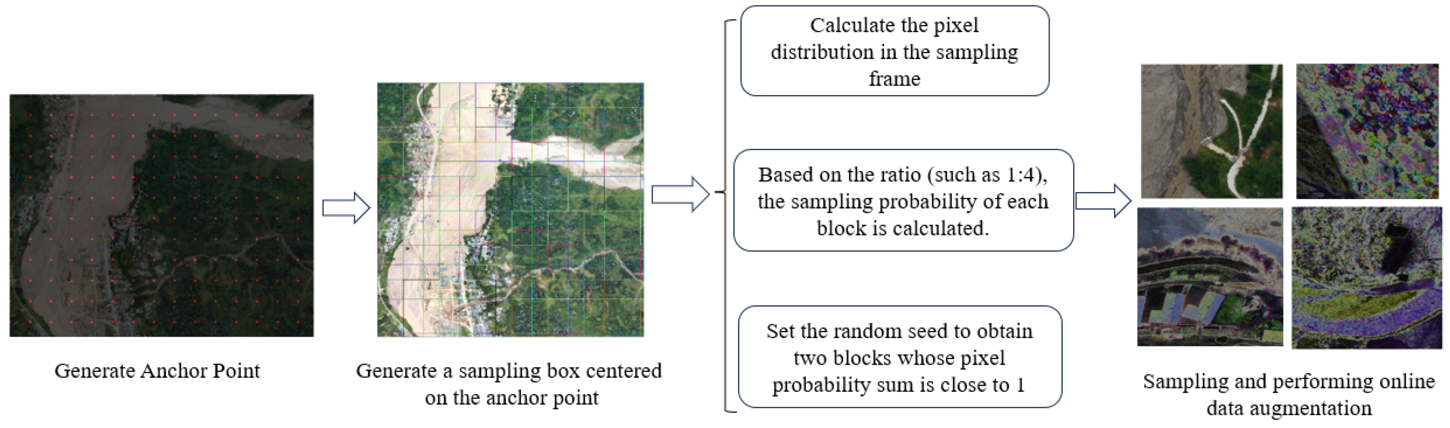
In order to verify the effectiveness of the balanced sampling method, a comparative experiment is set up and compared with non-sampling and uniform sampling.

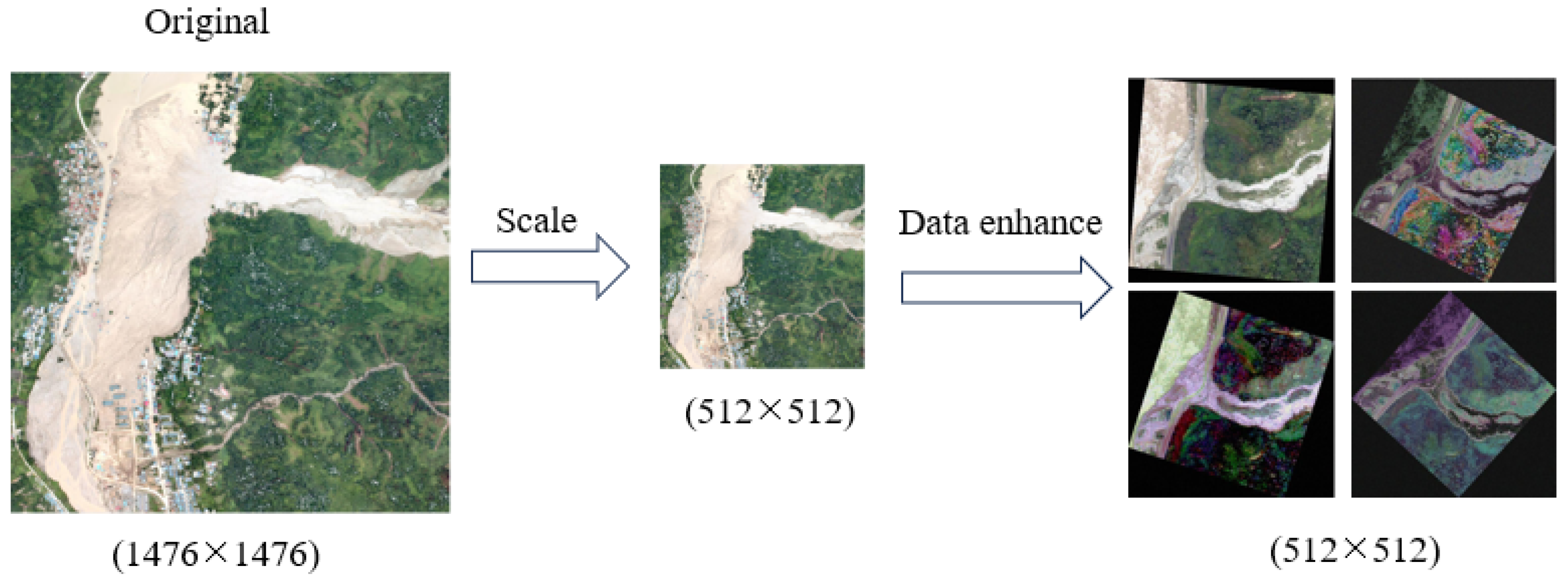
• NO: Reduce the image ratio to 512 × 512 and then use the online image enhancement method.
• Uniformity: Samples are sampled sequentially according to the anchor points, and the sample tile size is 512 × 512.
• Ours: Samples are sampled to balance the positive and negative samples in the dataset using the methods described in this article.

If the data length is the same, the specific metrics are in

Table 6. Comparison under different sampling methods.

Sampling Method	Precision (%)	Recall (%)	Dice (%)	mDice (%)
No	57.31	64.51	57.02	71.93
Uniformity	77.40	77.50	77.00	77.90
Ours	84.74	92.23	84.75	90.34

:

For this process, we compare a total of eight models using this public dataset. The models—specifically, U-Net, PSPNet, U-Net++, LinkNet [43], MAnet [44], DeepLabv3, DeepLabv3+ [45], and FPN [46]—are categorized alongside other generic semantic segmentation models using the same dataset. We use ResNet34 as the backbone network in these general models. To accelerate convergence, pre-trained weights are used; the base weights from the official pre-trained model are applied to the model proposed in this paper. After comparison, the specific indicators are in

Table 7. Comparison under different models.

Model	Precision (%)	Recall (%)	Dice (%)	mDice (%)
U-Net	80.61	95.95	79.32	86.84
PSNet	75.46	90.36	76.32	84.75
Unet++	76.62	90.75	78.37	86.21
LinkNet	74.86	95.41	76.77	85.12
DeepLabv3	77.86	92.34	79.55	86.92
DeepLabv3+	79.71	89.72	79.46	86.85
FPN	81.28	90.49	79.81	87.20
MAnet	75.25	90.10	78.86	86.32
Ours	84.74	92.23	84.75	90.34

, except for mDice, and the rest are the indicators on the validation set under the positive sample.

Table 6 illustrates the significant impact of different data processing methods on model performance. Specifically, the results of the first row show that the method is relatively ineffective. The main reason is that the scaling operation of the image will significantly weaken the model’s ability to perceive image features, and also reduce the efficiency of the model’s capture of contextual information, resulting in bias in the model’s feature extraction and understanding. For the results of the second row, we can see that this method leads to an imbalance in the distribution of data, and the ratio of positive and negative samples is unbalanced, which directly affects the training effect of the model. Unbalanced data can make the model tend to learn the features of the majority class and ignore the features of the minority, which will reduce the overall performance of the model. In contrast, our proposed balanced sampling method performs best across all metrics. This shows that balanced sampling can effectively balance the proportion of positive and negative samples, and ensure that the model can fully learn the features of each category during the training process. This balance not only improves the generalization ability of the model and enables it to better adapt to the data distribution in different scenarios, but also enhances the robustness of the model so that it can maintain stable performance in the face of complex data. Therefore, the balanced sampling method has significant advantages in improving the performance of the model.

The experimental results in Table 7 show the performance comparison between different models under the condition of consistent data augmentation methods and loss functions. Specifically, except for the recall rate, the other indicators of the proposed model are significantly better than those of other models. Among them, the Dice score is the core indicator for measuring the performance of the segmentation model, which directly reflects the accuracy and completeness of the model for the segmentation of the target area. The mDice score further integrates the overall segmentation ability of the model. Therefore, the excellent performance of the Dice score and the average Dice score fully demonstrate the excellent performance of the proposed model in the segmentation task. This shows that the proposed model can more accurately identify and segment the target area when dealing with complex boundaries and detail segmentation, especially in the segmentation of key categories (category 1). The results show that the proposed model has a significant advantage in segmentation ability, which not only balances the performance differences between different categories but also outperforms other models in key indicators, supporting the high efficiency and reliability of the model in practical applications. This further verifies the superiority of the proposed model in complex scenes and its potential in engineering applications.

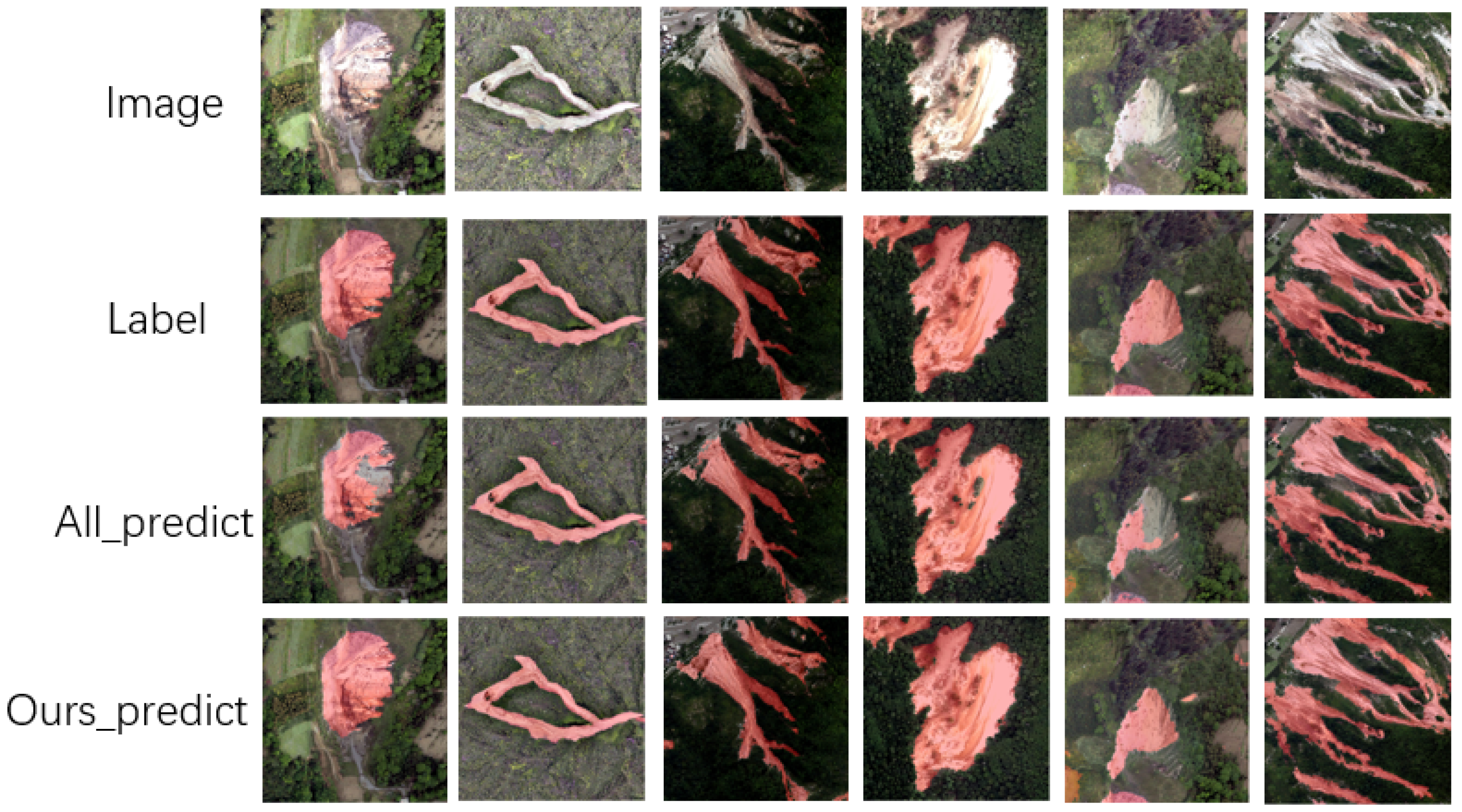
To comprehensively assess the model’s performance and conduct a thorough analysis, this paper selects three representative images with different regional characteristics in the validation set for predictive analysis. These images cover not only landslide disaster scenarios, but also other complex scenarios that are similar to the characteristics of landslides, such as roads and other natural or man-made objects that may resemble the morphology of landslides. This diverse selection of scenarios aims to more realistically simulate the challenges that the model may face in real-world applications while validating the model’s ability and robustness in distinguishing between different class features. The picture is shown in Figure 9:

Through the visualization of the labels and predicted images above, it can be observed that our model network outperforms other models. Compared to other CNN models, there may be some difficulties in processing global information. Our model employs a large kernel attention mechanism, enhancing the model’s perception of images from four aspects: local perception ability, long-distance dependency, spatial adaptability, and channel applicability, thereby extracting deep features of the images.

To better demonstrate the capabilities of the model, we visualize its output on the original image by generating a corresponding heatmap, as shown in Figure 10:

As can be seen from the figure, there are significant differences in the segmentation ability of different models when dealing with complex scenes. In the process of identification, some models have a high false positive rate (misjudging the non-landslide area as a landslide) and a false negative rate (missing the actual landslide area), which reflects their shortcomings in distinguishing the target features from the background interference. This phenomenon stems from the model’s limited ability to perceive local details of the image and the insufficient ability to capture long-distance dependencies.

In contrast, the model proposed in this paper performs well among all the comparison models. The main reason for this is that the large kernel attention mechanism is introduced into the model. This mechanism significantly enhances the model’s ability to perceive local features of the image, improves its ability to model long-distance dependence, and optimizes spatial adaptability and channel adaptability. Through this mechanism, the model can more accurately identify the subtle features of the landslide area and effectively suppress the interference of background noise, to achieve a more accurate segmentation effect in complex scenes.

4.2. Ablation Experiment

This section details ablation experiments that investigate the contribution and mechanism of each model module. In terms of experimental design, all ablation experiments were conducted based on the pre-trained model to ensure fairness and comparability of the experimental conditions. During the training process, each experimental group maintained 50 training rounds to fully evaluate the impact of each module on the performance of the model. By comparing the experimental results under different module combinations, we can quantitatively analyze the independent contribution of each component and its importance in the overall model.

In order to deeply analyze the impact of each module on the performance of the model, this study conducted a detailed split experiment on the loss function and decoder. Specifically, the loss function is deconstructed into Dice loss and labeled smooth limited cross-entropy loss (LCE), while the decoder is divided into the FPN module and CBAM module. Through ablation experiments on each module in turn, we observed that the method proposed in this paper has achieved significant improvement in the Dice index and the mDice index. The specific experimental data are shown in

Table 8. Ablation experiment of VanCASSP per module.

Encoder		Decoder		Dice (%)	mDice (%)
DiceLoss	LCE	FPN	CBAM
✓	✓	✓	✓	84.75	90.34
✓		✓	✓	80.40	87.50
	✓	✓	✓	80.52	87.90
✓	✓	✓		81.83	89.30

✓ is indicates that this module is selected

.

4.3. Post-Processing Comparison

Because most methods choose to conduct model training and prediction at low resolution, this often results in insufficient accuracy in the image assessment outcomes following landslide disasters. To restore the true resolution of aerial images, considering that the image resolution used during our training was 512 × 512, we adopted a strategy to ensure the model’s adequate perception of the images. Specifically, we sampled the predicted images with a step size of 256, dividing them into multiple image blocks of size 512 × 512, and sequentially input these image blocks into the model for prediction. After obtaining the prediction results of all image blocks, we re-fused these results based on the sampling coordinates to obtain the prediction results of the original image, and this process effectively smoothed the image. To intuitively demonstrate the effectiveness of this method, we conducted whole image prediction and image block stitching prediction with a step size of 256 and visualized the predicted images for both cases for comparison. The details are in Figure 11:

Through the comparison of the above figure, we can feel a significant difference between the whole graph prediction method and the prediction method we propose. Taking the first and fifth columns of the images as an example, there is an obvious lack of landslide area in the visualization results of the whole map prediction, but our prediction method can completely and accurately identify the entire landslide area. The root of this difference lies in how the model is trained and how well it perceives contextual information. Our model is trained on 512 × 512 size images, which enables the model to focus more on detailed information when processing high-resolution images but also leads to insufficient perception of global context information in whole map prediction. Looking further at the pictures in columns 3, 4, and 6, we can see that our prediction method is significantly better than the whole map prediction method in terms of detail processing. Not only does our method accurately identify the overall extent of the landslide area, but it also better captures the subtle structure and edge information within the area, resulting in better detail. This indicates that our prediction method can more effectively balance the relationship between local details and global information when dealing with complex scenarios, to achieve more accurate and reliable prediction results.

5. Discussion

This study explored landslide identification in depth around three key dimensions: data balance, model performance, and post-processing. Although some progress has been made, there are still many areas that can be optimized. Future research can be explored in the following directions:

• Multi-source data fusion: Utilizes high-resolution remote sensing images and integrates multi-source remote sensing data, such as synthetic aperture radar (SAR) and spectral data. Utilizes the penetrating capabilities of SAR data to obtain information on soil moisture and vegetation structure, which, when combined with optical images, improves the accuracy of landslide identification.
• Combined with multidisciplinary research: Currently, this methodology is only used for remote sensing images, and the impact range of landslides is affected by many factors such as rainfall, geological vibrations, etc. Multidisciplinary research on landslides is being carried out. For example, by combining this approach with geology, researchers can analyze the geological structure, rock properties, and stratigraphic distribution of the study area in detail, enhancing the analysis with remote sensing data to comprehensively understand the causes of landslides. Combining this approach with meteorology involves integrating meteorological data, including rainfall, rainfall intensity, rainfall duration, etc., to analyze their relationships with the scale of landslides.
• Combined with zero-sample generation technology: This approach uses zero-sample generation technology based on CLIP cross-modal alignment; the text description is mapped to the image feature space, enabling text-driven generation of landslide features in unseen areas. Through this technology, text features are aligned with image features to generate an image that matches the description. In the context of landslide data generation, it can solve the problem of scarce samples in remote areas and provide robust data support for research. In the future, this technology will continue to develop in terms of model efficiency, multi-modal fusion, and the expansion of application fields, providing more powerful technical support for the governance of landslide disasters.

6. Conclusions

In this paper, a new segmentation model based on Van–UPerAttnSeg is proposed for the landslide segmentation problem. In this process, a new data-sampling method is proposed to solve the problem of uneven data distribution. Compared with the two methods of no sampling and random sampling, it can be concluded that the balanced sampling method improves the generalization ability of the model.

In this paper, the model introduces a combination of label smoothing, maximum suppression cross-entropy, and Dice loss, which enhances the model’s convergence speed. Evaluation metrics such as the Dice score and average Dice score have shown improvement in comparison experiments with other common loss functions.

In terms of model comparison, this paper primarily compares eight classic models. For each metric, the proposed Van–UPerAttnSeg segmentation model has shown improvements over other models in the five evaluation metrics of Precision, Recall, Dice, and mDice presented in this paper.

All indicators in this article are calculated based on the original image, including high-resolution images. This article uses 512 × 512-sized patches for training to better adapt to the image’s field of view, and consequently, the predicted patch size is also 512 × 521. This approach not only better adapts the features of the patches but also reduces dependence on the GPU. Therefore, this article proposes a Gaussian fusion post-processing method, which is more meaningful for reference.

The research presented in this article highlights the excellent performance of the Van–UPerAttnSeg model in landslide segmentation tasks, and the proposed post-processing method holds significant importance for post-disaster assessment and reconstruction of landslides.

References

1. Langping, L.; Xingxing, L. Research on complexity of landslide motion paths: Review and prospects. Earth Sci. 2022, 47, 4663–4680. [Google Scholar]
2. Iverson, R.M. Landslide triggering by rain infiltration. Water Resour. Res. 2000, 36, 1897–1910. [Google Scholar]
3. Kamp, U.; Growley, B.J.; Khattak, G.A.; Owen, L.A. GIS-based landslide susceptibility mapping for the 2005 Kashmir earthquake region. Geomorphology 2008, 101, 631–642. [Google Scholar]
4. Salbego, G.; Floris, M.; Busnardo, E.; Toaldo, M.; Genevois, R. Detailed and large-scale cost/benefit analyses of landslide prevention vs. post-event actions. Nat. Hazards Earth Syst. Sci. 2015, 15, 2461–2472. [Google Scholar]
5. Ling, P.; Suning, X.; Junjun, M.; Fenghuan, S. Earthquake-induced landslide recognition using high-resolution remote sensing images. J. Remote Sens. 2017, 21, 509–518. [Google Scholar]
6. Lu, H.; Li, W.; Xu, Q.; Dong, X.; Dai, C.; Wang, D. Early detection of landslides in the upstream and downstream areas of the Baige Landslide, the Jinsha River based on optical remote sensing and InSAR technologies. Geomat. Inf. Sci. Wuhan Univ. 2019, 44, 1342–1354. [Google Scholar]
7. Tsai, F.; Hwang, J.H.; Chen, L.C.; Lin, T.H. Post-disaster assessment of landslides in southern Taiwan after 2009 Typhoon Morakot using remote sensing and spatial analysis. Nat. Hazards Earth Syst. Sci. 2010, 10, 2179–2190. [Google Scholar] [CrossRef]
8. Fiorucci, F.; Cardinali, M.; Carlà, R.; Rossi, M.; Mondini, A.; Santurri, L.; Ardizzone, F.; Guzzetti, F. Seasonal landslide mapping and estimation of landslide mobilization rates using aerial and satellite images. Geomorphology 2011, 129, 59–70. [Google Scholar]
9. Michael, P. LaValley. Logistic regression. Circulation 2008, 117, 2395–2399. [Google Scholar]
10. Schuldt, C.; Laptev, I.; Caputo, B. Recognizing human actions: A local SVM approach. In Proceedings of the 17th International Conference on Pattern Recognition, ICPR 2004, Washington, DC, USA, 23–26 August 2004; Volume 3, pp. 32–36. [Google Scholar]
11. Breiman, L. Random forests. Mach. Learn. 2001, 45, 5–32. [Google Scholar]
12. Tolga Can and Hakan, A. Nefeslioglu and Candan Gokceoglu and Harun Sonmez and Tamer Y. Duman. Susceptibility assessments of shallow earthflows triggered by heavy rainfall at three catchments by logistic regression analyses. Geomorphology 2005, 72, 250–271. [Google Scholar]
13. Chen, W.; Xie, X.; Wang, J.; Pradhan, B.; Hong, H.; Bui, D.T.; Duan, Z.; Ma, J. A comparative study of logistic model tree, random forest, and classification and regression tree models for spatial prediction of landslide susceptibility. Catena 2017, 151, 147–160. [Google Scholar] [CrossRef]
14. Landwehr, N.; Hall, M.; Frank, E. Logistic model trees. Mach. Learn. 2005, 59, 161–205. [Google Scholar] [CrossRef]
15. Dargan, S.; Kumar, M.; Ayyagari, M.R.; Kumar, G. A survey of deep learning and its applications: A new paradigm to machine learning. Arch. Comput. Methods Eng. 2020, 27, 1071–1092. [Google Scholar] [CrossRef]
16. Krizhevsky, A.; Sutskever, I.; Hinton, G.E. ImageNet classification with deep convolutional neural networks. Commun. ACM 2017, 60, 84–90. [Google Scholar]
17. Girshick, R.; Donahue, J.; Darrell, T.; Malik, J. Rich feature hierarchies for accurate object detection and semantic segmentation. In Proceedings of the IEEE Conference on Computer Vision and Pattern Recognition, Columbus, OH, USA, 23–28 June 2014; pp. 580–587. [Google Scholar]
18. Girshick, R. Fast r-cnn. arXiv 2015, arXiv:1504.08083. [Google Scholar]
19. Redmon, J.; Divvala, S.; Girshick, R.; Farhadi, A. You Only Look Once: Unified, Real-Time Object Detection. In Proceedings of the IEEE Conference on Computer Vision and Pattern Recognition, Las Vegas, NV, USA, 27–30 June 2016; pp. 779–788. [Google Scholar]
20. Liu, W.; Anguelov, D.; Erhan, D.; Szegedy, C.; Reed, S.; Fu, C.Y.; Berg, A.C. Ssd: Single shot multibox detector. In Proceedings of the Computer Vision—ECCV 2016: 14th European Conference, Amsterdam, The Netherlands, 11–14 October 2016; Proceedings, Part I 14. Springer: Berlin/Heidelberg, Germany, 2016; pp. 21–37. [Google Scholar]
21. Sameen, M.I.; Pradhan, B. Landslide detection using residual networks and the fusion of spectral and topographic information. IEEE Access 2019, 7, 114363–114373. [Google Scholar] [CrossRef]
22. Cheng, L.; Li, J.; Duan, P.; Wang, M. A small attentional YOLO model for landslide detection from satellite remote sensing images. Landslides 2021, 18, 2751–2765. [Google Scholar] [CrossRef]
23. Bochkovskiy, A.; Wang, C.Y.; Liao, H.Y.M. Yolov4: Optimal speed and accuracy of object detection. arXiv 2020, arXiv:2004.10934. [Google Scholar]
24. Xiaoting, J.; Kang, Z.; Xiaoqing, Z.; Qi, Z.; Wen, Z. Landslide hazard identification based on Faster R-CNN target detection—taking Fugong County urban area as an example. Ind. Miner. Process. Kuangwu Jiagong 2022, 51, 19–24. [Google Scholar]
25. Wang, T.; Liu, M.; Zhang, H.; Jiang, X.; Huang, Y.; Jiang, X. Landslide detection based on improved YOLOv5 and satellite images. In Proceedings of the 2021 4th International Conference on Pattern Recognition and Artificial Intelligence (PRAI), Yibin, China, 20–22 August 2021; pp. 367–371. [Google Scholar]
26. Tang, X.; Tu, Z.; Ren, X.; Fang, C.; Wang, Y.; Liu, X.; Fan, X. A Multi-Modal Deep Neural Network Model for Forested Landslide Detection. Geomat. Inf. Sci. Wuhan Univ. 2024, 49, 1566–1573. [Google Scholar]
27. Ronneberger, O.; Fischer, P.; Brox, T. U-net: Convolutional networks for biomedical image segmentation. In Proceedings of the Medical Image Computing and Computer-Assisted Intervention—MICCAI 2015: 18th International Conference, Munich, Germany, 5–9 October 2015; Proceedings, Part III 18. Springer: Berlin/Heidelberg, Germany, 2015; pp. 234–241. [Google Scholar]
28. Zhao, H.; Shi, J.; Qi, X.; Wang, X.; Jia, J. Pyramid scene parsing network. In Proceedings of the IEEE Conference on Computer Vision and Pattern Recognition, Honolulu, HI, USA, 21–26 July 2017; pp. 2881–2890. [Google Scholar]
29. Chen, L.C. Rethinking atrous convolution for semantic image segmentation. arXiv 2017, arXiv:1706.05587. [Google Scholar]
30. Badrinarayanan, V.; Kendall, A.; Cipolla, R. Segnet: A deep convolutional encoder-decoder architecture for image segmentation. IEEE Trans. Pattern Anal. Mach. Intell. 2017, 39, 2481–2495. [Google Scholar]
31. Soares, L.P.; Dias, H.C.; Grohmann, C.H. Landslide segmentation with U-Net: Evaluating different sampling methods and patch sizes. arXiv 2020, arXiv:2007.06672. [Google Scholar]
32. Fang, C.; Fan, X.; Zhong, H.; Lombardo, L.; Tanyas, H.; Wang, X. A Novel historical landslide detection approach based on LiDAR and lightweight attention U-Net. Remote Sens. 2022, 14, 4357. [Google Scholar] [CrossRef]
33. Li, Z.; Guo, Y. Semantic segmentation of landslide images in Nyingchi region based on PSPNet network. In Proceedings of the 2020 7th International Conference on Information Science and Control Engineering (ICISCE), Changsha, China, 18–20 December 2020; pp. 1269–1273. [Google Scholar]
34. Du, B.; Zhao, Z.; Hu, X.; Wu, G.; Han, L.; Sun, L.; Gao, Q. Landslide susceptibility prediction based on image semantic segmentation. Comput. Geosci. 2021, 155, 104860. [Google Scholar]
35. Yun, L.; Zhang, X.; Zheng, Y.; Wang, D.; Hua, L. Enhance the accuracy of landslide detection in UAV images using an improved Mask R-CNN Model: A case study of Sanming, China. Sensors 2023, 23, 4287. [Google Scholar] [CrossRef]
36. Dou, J.; Yunus, A.P.; Merghadi, A.; Shirzadi, A.; Nguyen, H.; Hussain, Y.; Avtar, R.; Chen, Y.; Pham, B.T.; Yamagishi, H. Different sampling strategies for predicting landslide susceptibilities are deemed less consequential with deep learning. Sci. Total. Environ. 2020, 720, 137320. [Google Scholar]
37. Liang, L.; Zhang, Z.M. Structure-aware enhancement of imaging mass spectrometry data for semantic segmentation. Chemom. Intell. Lab. Syst. 2017, 171, 259–265. [Google Scholar]
38. Domokos, C.; Kato, Z. Parametric estimation of affine deformations of planar shapes. Pattern Recognit. 2010, 43, 569–578. [Google Scholar]
39. Salvi, M.; Acharya, U.R.; Molinari, F.; Meiburger, K.M. The impact of pre-and post-image processing techniques on deep learning frameworks: A comprehensive review for digital pathology image analysis. Comput. Biol. Med. 2021, 128, 104129. [Google Scholar] [CrossRef] [PubMed]
40. Flusser, J.; Farokhi, S.; Höschl, C.; Suk, T.; Zitova, B.; Pedone, M. Recognition of images degraded by Gaussian blur. IEEE Trans. Image Process. 2015, 25, 790–806. [Google Scholar] [CrossRef] [PubMed]
41. Zeng, C.; Cao, Z.; Su, F.; Zeng, Z.; Yu, C. High-precision aerial imagery and interpretation dataset of landslide mudslide disasters in and around Sichuan (2008–2020). China Sci. Data 2022, 7, 191–201. [Google Scholar]
42. Li, H.; He, Y.; Xu, Q.; Deng, J.; Li, W.; Wei, Y. Detection and segmentation of loess landslides via satellite images: A two-phase framework. Landslides 2022, 19, 673–686. [Google Scholar] [CrossRef]
43. Chaurasia, A.; Culurciello, E. Linknet: Exploiting encoder representations for efficient semantic segmentation. In Proceedings of the 2017 IEEE Visual Communications and Image Processing (VCIP), St. Petersburg, FL, USA, 10–13 December 2017; pp. 1–4. [Google Scholar]
44. Fan, T.; Wang, G.; Li, Y.; Wang, H. Ma-net: A multi-scale attention network for liver and tumor segmentation. IEEE Access 2020, 8, 179656–179665. [Google Scholar] [CrossRef]
45. Chen, L.C.; Zhu, Y.; Papandreou, G.; Schroff, F.; Adam, H. Encoder-decoder with atrous separable convolution for semantic image segmentation. In Proceedings of the European Conference on Computer Vision (ECCV), Munich, Germany, 8–14 September 2018; pp. 801–818. [Google Scholar]
46. Lin, T.Y.; Dollár, P.; Girshick, R.; He, K.; Hariharan, B.; Belongie, S. Feature pyramid networks for object detection. In Proceedings of the IEEE Conference on Computer Vision and Pattern Recognition, Honolulu, HI, USA, 21–26 July 2017; pp. 2117–2125. [Google Scholar]
Figure 2. Online enhancement of blocks and online equalization sampling.
Remotesensing 17 01265 g002
Figure 3. Direct image scaling and online enhancement.
Remotesensing 17 01265 g003
Figure 4. Overview of the Van–UPerAttnSeg structure: The encoder part adopts a four-level stage architecture, and each stage consists of a hierarchical feature extraction structure composed of a block module and patch embed module to obtain four-level features, The decoder integrates the PPM module, FPN module, and CBAM module to fuse and enhance multi-level features.
Remotesensing 17 01265 g004
Figure 5. Encoder overview: The encoder uses the patch embed module to carry out multi-dimensional sampling on the input block to generate a characteristic batch with rich semantic information.Block integrates the large kernel attention module and MLP module to achieve multi-level feature extraction.
Remotesensing 17 01265 g005
Figure 6. Decoder overview: The decoder uses the ppm module to extract and fuse multi-level features, and the FPN module to fuse deep and shallow feature information to capture local details and global context information. The CBAM attention mechanism is introduced to adaptively weigh the fused features from the two dimensions of channel and space to further highlight key features and suppress redundant information.
Remotesensing 17 01265 g006
Figure 7. Overview of post-processing: Dense sampling by sliding window strategy, a weighted fusion of blocks in overlapping regions by the Gaussian kernel function.
Remotesensing 17 01265 g007
Figure 8. Visualization of annotation results of multiple orthophotos.
Remotesensing 17 01265 g008
Figure 9. Comparison of label predictions.
Remotesensing 17 01265 g009
Figure 10. Visualization of predicted images.
Remotesensing 17 01265 g010
Figure 11. Post-processed image visualization.
Remotesensing 17 01265 g011