Perfect Labelling: A Review and Outlook of Label Optimization Techniques in Dynamic Earth Observation

Abstract

Advances in Artificial Intelligence (AI) and Machine Learning (ML) have significantly enhanced the practice of Earth Observation (EO), enabling complex analyses such as land cover change detection, vegetation monitoring, and disaster response. However, while model architectures have matured, the refinement of reference data remains a major challenge. Accurate and dynamic multi-temporal labelling is essential for capturing evolving ground conditions in high-dimensional EO datasets, yet key challenges persist, including spatiotemporal inconsistencies, heterogeneous data integration, and multi-resolution harmonization. Without robust preprocessing, reference labels may introduce biases, resulting in reduced model reliability and generalizability. This review tackles four core aspects of reference data preprocessing in EO: (i) essential steps for producing consistent and high-quality datasets, particularly for dynamic spatiotemporal data; (ii) best practices and guidelines that enable scalable and accurate workflows across diverse EO applications; (iii) introduction of the HELIX framework, a unified approach for standardizing, enhancing, and automating spatiotemporal label preprocessing; and (iv) a forward-looking discussion on the future of reference labels and features, including next-generation techniques for dynamic EO data integration. By synthesizing existing methodologies, highlighting emerging approaches, and addressing current gaps, this review underscores how well-engineered reference data are fundamental to advancing AI/ML-driven EO applications.

1. Introduction

Earth Observation (EO) has become increasingly important for analysing and monitoring both climatic and anthropogenic changes. EO data acquisition is supported by rapid advancements in remote sensing technologies and leverages diverse platforms; satellites offer global coverage and continuous time series data [1], whereas airborne systems (including drones) provide data with higher spatial resolution for targeted areas. Remote sensing devices are broadly grouped into passive sensors for capturing reflected or emitted natural radiation (for instance, optical or thermal sensors) and active sensors such as radar and LiDAR that emit their own energy and record the backscattered signal [2]. These techniques generate multi-source data with varying spatial, temporal, and spectral resolutions, requiring sophisticated integration methods for coherent analysis. As a result, EO data form the basis for studying dynamic processes such as climate change, urbanization, and natural resource management. These data underpin practical tasks ranging from vegetation monitoring and wildfire assessment [3] to crop yield prediction and irrigation optimization [4], as well as urban growth analysis and traffic flow management [2], among others.

The transformation of raw EO data into actionable insights depends on high-quality reference data obtained from ground measurements or semantic maps. These reference data are essential for Artificial Intelligence (AI) and Machine Learning (ML) model training, validation, and testing [5]. Whether obtained directly from EO or compiled via ancillary sources, reference data act as a crucial link or a translator between raw EO observations and model interpretation, ensuring that algorithms correctly associate input features with real-world conditions [6]. By mapping pixel values, spectral signatures, or spatial structures to known labels, reference data provide the necessary foundation for supervised learning tasks, including land cover classification, object detection, and change monitoring. Without representative reference data that have been properly preprocessed and balanced [7], AI/ML models risk learning biased, inconsistent, or erroneous patterns, ultimately compromising their reliability and generalizability in EO applications [8]. Therefore, common classification approaches sometimes perform signature refinement in order to cope with possible errors in the reference data [9].

Reference data can be static (collected at a single date) [10,11,12], multi-temporal (collected at several dates but labelled as a single class) [13], or fully dynamic [14], capturing changes across multiple time steps. Dynamic labelling demands specialized methods to ensure multi-temporal consistency, particularly for tasks such as land cover classification, object detection, and anomaly detection. The performance of ML models, including traditional approaches such as Decision Trees (DT), Support Vector Machines (SVM), and Random Forests (RF) as well as Deep Learning (DL) architectures based on Convolutional Neural Networks (CNN), are highly dependent on the quality and comprehensiveness of reference data. High-quality and accurately labelled datasets are essential for the capture of spatial, spectral, and temporal complexities, which in turn ensure model reliability and generalization [15]. Given that Foundation Models (FM) are built upon large-scale datasets for pretraining and adaption, their effectiveness is also inherently tied to data quality [16,17]. Traditional models offer interpretability with structured datasets [18], whereas DL excels in extracting complex features but relies on large labelled datasets [19].

In recent years, the proliferation of temporal reference data has transformed the landscape of remote sensing, environmental monitoring, and other fields that rely on spatiotemporal analysis. The increasing availability of satellite imagery, sensor networks, and time series records offers unprecedented opportunities to model dynamic processes over space and time. However, the sheer volume and complexity of these data pose significant challenges for traditional analytical methods, which are frequently designed for static datasets. By nature, temporal reference data capture changes over time, offering a dynamic view of the phenomena under study. Although invaluable, this also introduces a layer of complexity that is absent in static datasets. Temporal data are inherently multidimensional, involving regular to almost continuous measurements across time, space, or even additional dimensions such as depth or elevation. Accounting for temporal dependencies, spatial correlations, and multidimensional interactions is essential for extracting meaningful insights, highlighting the need for preprocessing frameworks tailored specifically to temporal reference data. Preprocessing reference data in EO is particularly challenging due to temporal inconsistencies, missing or noisy measurements, and the need to harmonize inputs from multiple sources [4]. These challenges are amplified in dynamic datasets, where time-stamped labels, shifting class boundaries, and irregular sampling all demand robust workflows. Studies have estimated that data preprocessing tasks account for 50–80% of the AI or ML workflow [20], underscoring their importance.

Despite the importance of refining reference data, this issue has received considerably less attention than model development. While advancements in DL architectures and model optimization have dominated EO research, systematic approaches for handling, standardizing, and preparing reference datasets remain underexplored. Traditional ML models are not inherently equipped to handle the temporal and spatial dependencies present in temporally variable reference data. These methods typically assume that the input features are independent, an assumption that is often violated in spatiotemporal contexts. Without appropriate preprocessing, such models may overlook the underlying temporal dynamics and spatial relationships, yielding suboptimal performance or misleading conclusions [21,22]. This challenge becomes even more pronounced when dealing with multi-temporal satellite imagery sources such as fused optical and SAR datasets, where differing temporal sampling and external factors (for example, weather conditions that obscure the optical imagery) can create missing data or misalignment. Ensuring that all data sources remain temporally aligned and that any temporal dependencies are appropriately captured is key for enabling traditional ML models to discover meaningful patterns, as these models are not natively able to handle temporal sequences.

1.1. General Differences in Label Preparation by Model Type

Label preparation is fundamental to the success of ML, DL, AI, and FM in EO applications. However, the ways in which reference data are prepared, structured, and utilized vary significantly across these model types. These differences arise due to variations in feature extraction requirements, data volume, annotation strategies, and the need for static or dynamic labels.

Common ML models rely heavily on manually curated reference data [23] to establish relationships between predictor variables and target outputs. These models require well-structured predictor–label pairs, and reference data quality plays a crucial role in ensuring model reliability [24]. In EO applications, domain experts define features such as spectral indices. Such indices include the Normalized-Difference Vegetation Index (NDVI), spatial texture metrics, and aggregated temporal statistics such as vegetation indices over a growing season [25]. These models assume that data points or pixels are independent unless temporal dependencies are explicitly introduced through engineered features. Because ML models require structured training data, label preparation often involves a meticulous manual annotation or expert-driven classification process [24].

A key advantage of ML models is their ability to perform well with smaller datasets when meaningful and structured features are available [24]. However, the reliance on manually crafted features and static training labels limits ML’s flexibility when applied to highly complex, multi-temporal, or multi-source EO datasets. Because conventional ML models lack the ability to automatically extract hierarchical features from raw data, their performance is heavily dependent on the quality and completeness of the reference data. Despite the pivotal role of preprocessing temporal reference data, research on these steps for traditional ML models such as RF remains limited, even though they are widely used in EO [26]. Poor preprocessing can introduce inconsistencies [27], yet comprehensive guidelines for handling multi-temporal reference data in traditional ML are still lacking.

While DL models often include structured preprocessing pipelines, similar frameworks for classical models such as RF are underexplored. Most of the literature on handling time series data focuses on specialized models such asLong Short-Term Memory (LSTM), a type of Recurrent Neural Network (RNN) specializing in long-term dependency modelling, which leaves a gap around simpler yet powerful methods that can be adapted to spatiotemporal complexities [28]. This gap underscores the necessity for further innovation in preprocessing approaches that reconcile the demands of dynamic multidimensional EO datasets with the operational simplicity and lower computational footprint of classic algorithms.

Overall, failing to capture or correctly process temporal and spatial dependencies can yield biased estimates and reduced predictive power. As data volume continues to grow, robust and efficient workflows for creating and maintaining dynamic reference datasets will become even more essential. A lack of standardized and scalable methodologies for handling time-sensitive or multidimensional EO data effectively undermines the potential of even the most sophisticated AI/ML architectures. Addressing this concern requires automating dynamic labelling, mitigating data inconsistencies introduced by multi-sensor fusion, and explicitly integrating spatiotemporal dependencies into the preprocessing pipeline.

In contrast, DL models can learn representations directly from raw EO data, eliminating the need for explicit label engineering [15]. CNNs, RNNs, and Temporal Convolutional Networks (TempCNNs) operate on high-dimensional datasets such as multispectral time series, learning hierarchical patterns from large-scale annotated datasets [29]. While ML approaches typically rely on structured discrete class labels, DL models demand pixel-wise or spatially dense annotations, particularly for tasks such as land cover classification and semantic segmentation.

Unlike ML, which can cope with relatively small datasets if structured features are available, DL models require extensive training data in order to generalize. This poses a significant challenge in EO applications, where obtaining high-resolution expert-annotated reference data is a time-intensive and costly process [30]. In many cases, researchers employ synthetic data generation, transfer learning, or pretraining on related datasets to mitigate the lack of labelled samples. Furthermore, inconsistencies introduced by human annotators can significantly affect DL model performance, requiring strict quality control during the labelling process.

FMs introduce a fundamental shift in AI-based EO applications, addressing many of the limitations of ML and DL models in terms of reference data preparation [16]. Unlike traditional AI approaches, which require manually labelled datasets, FMs leverage large-scale self-supervised learning to learn feature representations without relying on explicit annotation. Recent advances involving FMs include the Segment Anything Model (SAM) [31], a promptable segmentation model capable of generating high-quality masks for any image region without task-specific training, and DINO [32], a self-supervised vision transformer trained without labels. These models have demonstrated the ability to generate pixel-wise labels automatically, significantly reducing the need for manual labelling. FMs demonstrate strong adaptability in handling label noise and evolving class definitions, thereby reducing reliance on static reference labels in multi-temporal EO applications. In dynamic task environments such as land cover change detection and vegetation monitoring, where traditional labels quickly become outdated, FMs leverage self-supervised learning to refine and adapt training labels over time. Models such as Changen2 [33] can generate supervisory signals for label correction, while recent evaluations have shown that FMs remain label-efficient and generalize well in EO applications even under limited annotation scenarios [34,35]. Unlike DL models, which require fine-tuning with extensive labelled datasets, FMs can generalize more effectively, adapting to new classes with minimal labelled examples through few-shot or zero-shot learning [36,37].

While the labelling needs of ML, DL, and FM approaches differ, various methods have been developed to mitigate dependence on exhaustive manual annotation.

Table 1. ML methods for reducing dependency on exhaustive labelled datasets.

Method	Key Mechanism	Applications in EO
Transfer Learning	Adaptation of models pre-trained on related tasks to EO-specific problems [39,40].	Land cover classification, drought assessment [39].
Self-Supervised Learning	Creation of supervisory signals from within the data itself, enabling feature learning [41].	Vegetation monitoring, anomaly detection [41].
Active Learning	Th model identifies high-uncertainty samples and queries experts for targeted labelling [42].	Semantic labelling, urban morphology analysis [42].

summarizes these key techniques and their applications in EO. Despite their differences, both ML and DL approaches require robust reference data preparation to ensure training accuracy. In ML, manual feature engineering remains a crucial step, demanding consistency across datasets and expert domain knowledge in order to define meaningful features. In contrast, DL’s reliance on massive training datasets makes label availability, annotation quality, and scalability primary concerns. While ML models excel in well-defined structured scenarios where labelled data are limited, DL models thrive in high-dimensional data-rich environments where learning complex spatial and temporal patterns is essential [38].

1.2. Nature and Temporality of Labels

Labels are not singular entities; rather, they exist across multiple dimensions, and as such vary in terms of their type, scale, and temporal dynamics. Understanding of these dimensions is crucial for designing effective models that generalize well across different spatial and temporal contexts. In many cases, multi-output ML and DL models must simultaneously handle multiple target variables, necessitating structured approaches to label representation. These models rely on clearly defined label types to extract meaningful relationships across different scales and temporal dependencies. To systematically describe the nature of labels, we classify them based on their measurement scale, temporal behaviour, and attribution structure.

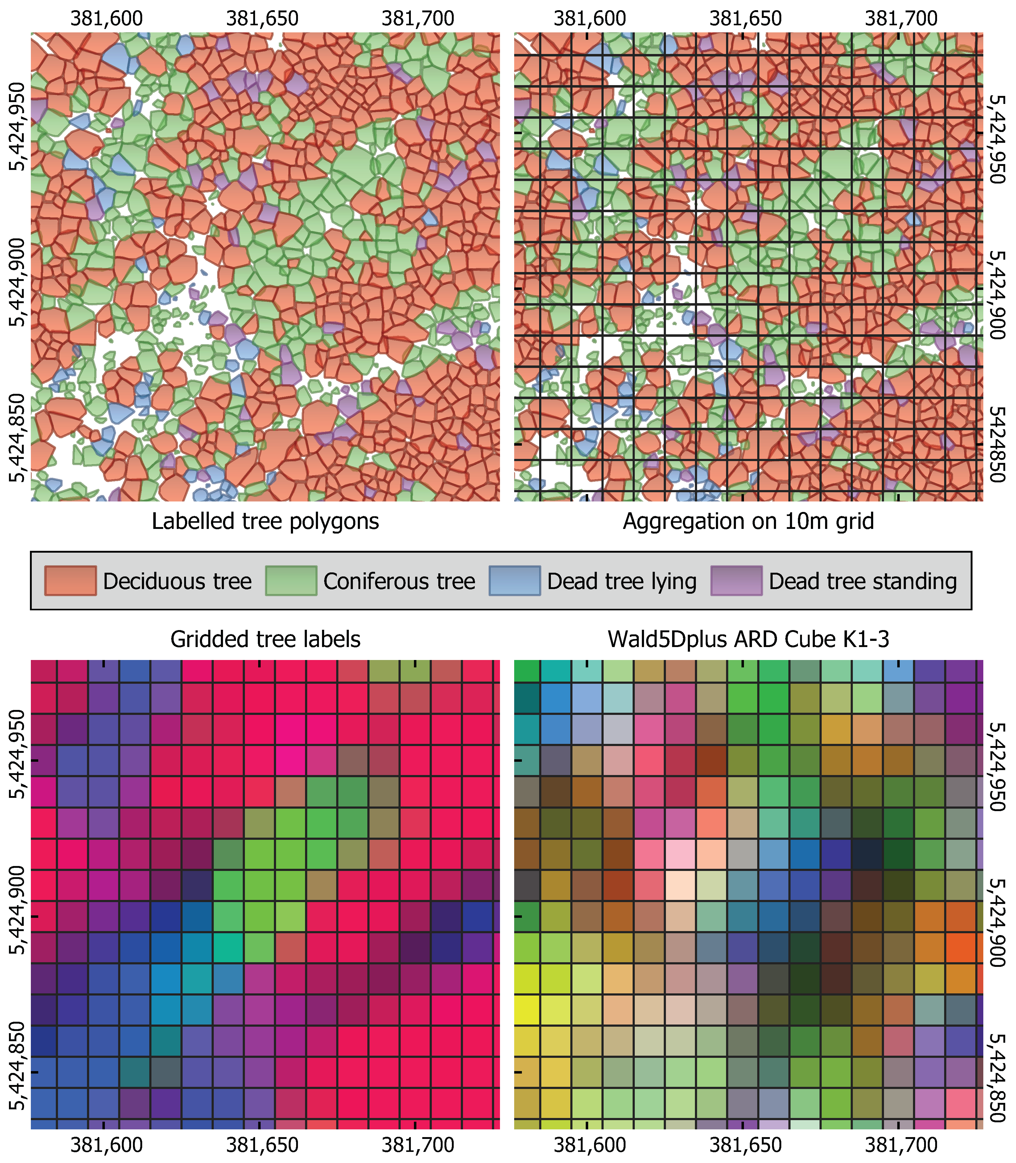
The structured reference labels presented in

Table 2. Example of structured reference labels for tree polygons in an example attribute table, with the respective scale level assigned in the last row.

ID	Type	Species	Age	Height	Infestation	Date	Not Before–Not After
1	Coniferous	Norway Spruce	Young	6 m	Yes	2025-03-03 14:49:43	2024-03–2025-03
2	Deciduous	Oak	Mature	12 m	No	2024-09-15 09:42:39	2023-09–2024-09
3	Coniferous	Scots Pine	Mid-age	8 m	No	2023-06-22 13:19:27	2022-06–2023-06
4	Deciduous	Beech	Young	5 m	Yes	2022-12-11 07:57:29	2021-12–2022-12
5	Coniferous	Douglas Fir	Mature	20 m	No	2023-05-18 10:02:11	2022-05–2023-05
6	Deciduous	Birch	Mid-age	9 m	Yes	2024-07-07 08:26:48	2023-07–2024-07
7	Coniferous	Larch	Mature	15 m	No	2023-08-30 11:23:46	2022-08–2023-08
⋮	⋮	⋮	⋮	⋮	⋮	⋮	⋮
	nominal	nominal	ordinal	relational	binary	continuous	interval

offer a comprehensive example for categorizing tree polygons into clearly defined data types, supporting systematic analysis in EO applications. Each data type reflects distinct measurement scales, analytical characteristics, and temporal implications. Because these labels are often derived from multi-source reference datasets such as field surveys, airborne LiDAR, and multi-temporal satellite imagery, they integrate numerical properties such as height, biomass, and spectral reflectance as well as categorical attributes such as species, tree type, and vegetation health. In addition to these, environmental and climate-related labels may include variables such as soil moisture, atmospheric conditions, and ecological succession stages, all of which require tailored preprocessing to ensure consistency across datasets.

Nominal data refer to categories without inherent order, such as “Tree Type” (coniferous or deciduous) and “Species” (e.g., Norway Spruce, Oak, Douglas Fir). These labels facilitate forest type classification and biodiversity assessments by clearly distinguishing distinct groups without implying any ranking or hierarchical structure. Ordinal data consist of labels organized into ranked categories, where the order signifies progression or intensity without requiring equal numerical intervals. Examples in the provided dataset include “Age” (categorized into growth stages such as young, mid-age, or mature) and “Height” (measured in meters), which indicate relative growth status from shorter to taller trees. These ordinal categories enable assessments of forest structure and succession stages. Relational data represent associations or relationships, such as those indicating spatial or contextual interactions between labelled entities or their environment. However, in this provided table, the relational aspect appears limited or not explicitly defined. If intended, relational labels might indicate proximity or contextual relationships, such as adjacency to disturbed areas, roads, or water bodies. Such information would need explicit representation, which appears missing from the current table. Binary data contain only two possible states, typically representing “yes/no” or “presence/absence” conditions. The provided example dataset includes an infestation status indicating whether a tree is infested (“Yes”) or not (“No”). This binary categorization directly supports analyses of forest health, infestations, and risk assessments related to pest outbreaks. Continuous data represent values measured on a numerical scale with precise and meaningful intervals. The provided table uses continuous data in the form of the exact “Date” of observation (e.g., “2025-03-03 14:49:43”), enabling precise temporal alignment with remote sensing observations or environmental events. Interval data define ranges or timeframes, specifying periods during which labels remain valid or applicable. In this dataset, the “Not Before–Not After” attribute (e.g., “2024-03–2025-03”) indicates the temporal validity or applicability of the label. This ensures temporal consistency during analyses, especially when integrating multiple sources of satellite data collected at different intervals or for long-term environmental monitoring. Together, these structured labels provide a clear and coherent basis for preprocessing reference data, thereby facilitating accurate analysis and consistent integration across diverse EO datasets and model types.

The temporality of the labels themselves is another factor which significantly affects the model’s ability to generalize and adapt to evolving conditions. Static labels are often insufficient for tasks that involve temporal variability, while dynamic labels enable more robust modelling of time-sensitive phenomena. Static labels are typically created for one-time use, and are suitable for environments with minimal change. Examples include static land cover maps, topographical surveys, and soil type classifications. In such cases, ML models can perform well if the input data remain aligned with these static labels. However, static labels become problematic in dynamic environments characterised by temporal phenomena such as seasonal vegetation changes, urban development, or disaster events [43].

For instance, in vegetation monitoring, static labels fail to account for fluctuating indices which track plant health over time, such as the NDVI and Enhanced Vegetation Index (EVI). Seasonal cycles comprising phases such as green-up, peak biomass, and senescence introduce temporal variability that static datasets are unable to represent. As a result, models trained with static labels may generalize poorly across seasons. Dynamic labelling, which continuously updates reference labels to reflect real-time changes, enables models to effectively capture phenological events and seasonal cycles, thereby enhancing long-term predictive accuracy.

For example, TempCNN has been successfully employed for vegetation monitoring. By integrating time-stamped labels, TempCNN networks have shown the ability to detect complex seasonal patterns in Sentinel-2 time series data [29]. However, the observed performance gains of TempCNN over RF and RNN (1–3% higher overall accuracy) in the aforementioned study were attributed to its ability to model temporal dependencies in Satellite Image Time Series (SITS) rather than to differences in labelling. The study compared different model architectures while keeping the reference labels fixed for validation and testing, meaning that the accuracy gains reflect architectural improvements rather than an effect of dynamic labelling. While dynamic labels have been shown to improve generalization in long-term monitoring tasks, their impact was not among the variables tested in this specific study.

Similarly, dynamic labels are critical for land use and land cover change detection. In the So2Sat LCZ42 dataset, dynamic Local Climate Zone (LCZ) labels were periodically updated to account for urban infrastructure development and population shifts across 42 global regions. This approach allowed models to consistently analyse urban morphology while minimizing errors caused by label obsolescence [13].

1.3. Challenges in Dynamic Labelling

Dynamic labelling frameworks often employ pseudolabelling and active learning, in which labels are iteratively refined based on model predictions and feedback from new observations [30]. These strategies are particularly effective in scenarios requiring adaptive label handling, such as drought monitoring, flood mapping, and crop assessment [44]. Their role in structuring training samples for EO classification has also been emphasized in broader reviews of remote sensing preprocessing techniques [45]. Incorporating dynamic reference data, which captures temporal variations, is essential for improving model adaptability in EO applications. Although easier to manage, static labels often fail to represent rapidly changing conditions such as those found in disaster monitoring or seasonal land cover dynamics. By contrast, spatiotemporal labelling strategies allow models to learn from evolving patterns, resulting in improved classification robustness and generalization across time [46]. Dynamic data include variables that evolve over time, such as daily temperature, precipitation, and vegetation indices. Dynamic reference data are essential for capturing temporal patterns, making them critical for applications such as crop monitoring and phenology-related studies. However, dynamic data require more sophisticated handling in order to maintain temporal dependencies, and integration with static data can be complex [46,47].

To summarise, unlike static reference data, dynamic labels evolve over time, enabling ML, DL, and/or AI models to track and predict real-world changes in land cover, vegetation growth, and natural disasters. This flexibility is substantial in applications where past conditions may no longer be representative of the present, such as deforestation monitoring, crop growth assessment, and flood detection. In consequence, the transition from static to dynamic reference data introduces several challenges related to temporal consistency, data quality, computational efficiency, and model adaptability. These challenges must be addressed in order to fully leverage dynamic labelling in EO applications. In this review, we tackle four main aspects of reference data preprocessing that are involved in, but not limited to, the dynamic EO data context:

(i)

The essential steps needed to produce consistent high-quality reference datasets, with a particular focus on handling dynamic spatiotemporal data and label engineering (Section 2).

(ii)

The challenges and limitations of reference label quality, consistency, and temporal alignment, demonstrated through practical cases in EO applications. We highlight key issues encountered in label preprocessing before presenting best practices and practical guidelines that enable scalable and accurate workflows across diverse EO applications (Section 3).

(iii)

Introduction of the HELIX framework, a unified framework for spatiotemporal label preprocessing designed to standardize, enhance, and automate EO-based training data preparation (Section 4.1).

(iv)

A forward-looking discussion on the future of label data and features, including next-generation labelling techniques for dynamic EO data integration (Section 4.2).

By synthesizing current methodologies, highlighting emerging approaches, and identifying gaps that warrant further investigation, we demonstrate how thoroughly engineered reference data, whether static or dynamic, can significantly enhance AI/ML-driven insights in time-sensitive and high-dimensional EO scenarios. A concise summary (Section 5) concludes the article.

2. Methodologies in Data Labelling and Processing

The mutual adaption of features and labels is crucial to any data-driven applications, serving as the foundation for effective data analysis. This holds true across various domains, including remote sensing. While labelling has been an interactive task for a long time in the case of deterministic classification methods such as Maximum Likelihood Estimation (MLE), the need for automated labelling strategies increases with the increased use of ML and DL techniques. Reference data are often affected by incompleteness, noise, inconsistencies, and multi-source integration challenges, all of which can reduce a model’s performance if not properly addressed.

Table 3. Challenges in reference data collection and their implications.

Problem Category	Specific Issues	Implications for Models
Excessive Data Complexity	High-dimensional feature space, irrelevant attributes, large dataset sizes [48], mixed categorical/numerical data, noisy measurements.	Increases computational burden and risk of overfitting; requires dimensionality reduction, feature selection, and data filtering to retain relevant information.
Insufficient Data Coverage	Missing values, small sample size, incomplete or underrepresented attributes in labels [48,49,50].	Leads to poor model generalization and increased overfitting risk; necessitates imputation, data augmentation, or synthetic data generation to ensure robustness.
Inconsistent and Heterogeneous Data	Incompatible data formats, multi-source integration challenges [51], discrepancies in spatial and temporal resolutions.	Introduces inconsistencies in training data; requires harmonization, resampling, and normalization techniques to ensure data consistency and compatibility across datasets.

provides a structured summary of these challenges and their implications. The following sections then span the basic requirements for labels and present common methods for label engineering, followed by a discussion of the simultaneous use of labels and features.

2.1. Requirements for Labels

Given the challenges outlined in Table 3, remote sensing reference data must meet specific requirements in order to ensure accuracy, consistency, completeness, and temporal relevance in AI- and ML-driven applications. Given the high level of accuracy needed for predictions across spatial and temporal scales, the requirements for reference data are stringent.

Ensuring that a model learns the correct mapping between input features (such as satellite imagery) and target outputs (labels such as land cover types or tree height) requires highly accurate reference datasets. Inaccurate reference data can introduce systematic errors, resulting in unreliable or misleading predictions. For example, misclassified land cover data could lead to incorrect estimates of deforestation rates or vegetation health [52]. Consistency across different datasets and time periods is equally important. In EO, where data is sourced from multiple sensors, discrepancies can introduce noise and degrade model accuracy. This issue is particularly critical when merging datasets collected at different times or from varied sensors, which may exhibit radiometric differences unless properly calibrated. Ensuring data harmonization through preprocessing techniques is essential for model generalization. Completeness of reference datasets is another key requirement. In cases where data are incomplete, imputation methods such as K-nearest neighbours or DL-based techniques can be used to reconstruct missing values, although these methods introduce uncertainties [53]. Temporal relevance plays a pivotal role when dealing with dynamic environmental variables. Models trained on outdated or temporally misaligned data may yield erroneous predictions as environmental patterns shift over time. This is particularly critical in applications such as deforestation monitoring, precision agriculture, and phenological studies, where multi-temporal reference data significantly enhances classification accuracy and model robustness by capturing seasonal variations and land cover dynamics [54]. Studies have shown that leveraging multi-temporal datasets improves classification performance by reducing errors associated with single-date observations, which may not fully capture environmental variability [54]. However, single-date reference data remain valuable for classification tasks where short-term assessments or immediate land cover mapping are required. The aforementioned study successfully classified crop types using vegetation indices from a single RapidEye image, demonstrating that while single-date datasets provide meaningful insights, they have inherent limitations in capturing temporal variations [55].

In addition to these factors, reference data must be suitable for the specific task at hand. Furthermore, dynamic reference data in remote sensing applications often need to reflect evolving environmental conditions. Proper label engineering techniques must be employed to ensure multi-temporal consistency of the reference labels in order to prevent temporal drift that may negatively impact ML models. Several key requirements must be met to ensure that these datasets support robust and unbiased analyses.

Table 4. Requirements for reference data in remote sensing.

Key Requirement	Definition and Practical Implications
High-Quality and Well-Labelled Data	Accurate and precisely labelled data are crucial for reliable model training and validation, ensuring that ML/DL models produce trustworthy predictions [56]. Poor-quality or inconsistent labels can bias analyses, underscoring the need for systematic quality control measures such as expert validation or crowdsourced labelling.
Accessibility of Public Datasets	Openly accessible reference datasets (with validation data) facilitate benchmarking and comparison against state-of-the-art methods [57,58,59]. Limited availability of high-quality datasets slows progress, highlighting the importance of open data policies and standardized validation samples.
Diversity and Representativeness	Training data must capture a wide range of environmental conditions (e.g., multiple land covers, seasonal variations) to enable robust generalization [60]. A narrowly focused dataset risks overfitting, whereas data augmentation and multi-source integration broaden variability to enhance model resilience.
Spatial and Temporal Coverage	Datasets should span large geographic areas and multiple acquisition dates to capture relevant spatial and temporal dynamics [2,60]. Missing spatial or temporal intervals can hinder model learning; interpolation and fusion techniques may alleviate coverage gaps.
Data Resolution	Aligning the spatial and temporal resolution of training samples with the resolution of remote sensing data preserves critical details [59]. Mismatched resolutions can obscure fine-scale features, potentially degrading model performance.
Quantity and Sample Size	An adequate number of training samples is essential for avoiding underfitting and improving model accuracy [48,50,56,61]. Insufficient sample sizes undermine model robustness; active learning and synthetic data generation can expand small datasets.
Consistency and Continuity	Maintaining consistent labelling protocols and data quality is vital for reliable analyses, especially across multiple sources or in time series contexts [2]. Inconsistent standards introduce noise, reducing a model’s predictive reliability over time.
Annotated Metadata	Comprehensive metadata (e.g., source, acquisition date, preprocessing steps) improve dataset interpretability and aid in reproducibility [59,62]. Missing or incomplete metadata can impede data harmonization and limit re-usability in future studies.
Data Balance	Balanced class distributions (e.g., for different land covers) minimize prediction bias [2]. Oversampling, undersampling, and synthetic data generation techniques are frequently employed to address skewed data and improve model fairness.

summarizes the essential requirements that reference datasets should meet in order to be effective for model-based remote sensing tasks.

2.2. Label Engineering

Because EO data form the basis for many labels in the geoinformation context (e.g., the CORINE land cover maps of the Copernicus program [63]), reference labels in EO datasets may not always be as completely independent as desired. In addition, EO data are generally prone to data quality issues such as missing values, noise, and redundancy, which can propagate into the labelling process and potentially bias downstream ML and DL models. This subsection focuses on how preprocessing steps ranging from gap-filling to data fusion can support the production of accurate and consistent reference datasets. Missing values are common in EO-derived labels due to temporary sensor outages, atmospheric interference (e.g., cloud cover), and irregular data collection intervals. Effective interpolation methods help to mitigate these gaps by estimating or reconstructing missing label information.

For reference labels that evolve seasonally or exhibit complex temporal dynamics, advanced smoothing (e.g., Savitzky–Golay) can help to retain longer-term patterns while filtering short-term fluctuations [64]. These methods are crucial in applications such as phenological monitoring, where incomplete or noisy label data may otherwise obscure subtle vegetation changes. Because reference labels in EO can represent diverse data types, including land cover classes, vegetation indices, temperature, or biophysical parameters, they may inherit noise from sensor limitations, atmospheric disturbances, or inconsistencies in manual or automated annotation. Strategies for mitigating these issues include filtering techniques in raster-derived labels such as Gaussian smoothing, which is suitable for reducing random noise, as well as median filtering, which is suitable for removing outliers while preserving major structural features. When constructing reference datasets, one sensor alone may not achieve the necessary spatial or temporal resolution. Thus, data fusion leverages complementary information, such as combining high-resolution Landsat imagery with frequent MODIS observations, in order to generate more complete and robust labels [65].

Table 5. Label engineering techniques.

Method	Key Mechanism	Effects in EO
Raster Aggregation	Sums up labels from neighbouring pixels to form a coarser but smoother raster.	Useful for creating coarse yet stable label datasets in complex terrains [66].
Segment Aggregation	Aggregates measurements on predefined reference polygons, stabilizes label assignment, and enhances thematic consistency	Forest stands or field parcels in land-cover classification or object-based labels [67].
Cross-Sensor Interpolation	Combines different data sources with varying characteristics to enhance the temporal sampling.	Bridging Landsat revisits [68], densifying NDVI time series [69], and glacier dynamics [70].
Spatiotemporal Filtering	Smooth continuous labels via spatiotemporal aggregation for noise reduction.	Removes short-term variations in meteorological measurements [71].
Normalization	Standardizing value range, semantic depth, numerical coding, etc.	Supports comparability and transferability.
Outlier Detection	Identifies and removes single inconsistent or improbable values within the labels.	Sensor failure or wrong timestamps in ground truth data [72].
Systematic Errors	Identifies and corrects for systematic deviations in the labels.	Overestimation of local temperature when using crowdsourced data [73].

outlines typical strategies.

Outliers in reference labels occur when inconsistent or improbable values emerge within the labelled dataset itself. For instance, if a crop type label assigned in a given year contradicts known crop rotation patterns or historical land use records, this may indicate a labelling error. Similarly, reference biomass values that deviate significantly from expected seasonal trends may suggest inconsistencies in the labelling process. Identifying and correcting such outliers using statistical validation, spatial consistency checks, or ML-based anomaly detection can enhance label quality before model training.

In addition to outlier correction, data fusion strategies enhance label consistency and accuracy in large-scale or long-term monitoring. Table 5 outlines key methods used to stabilize reference labels and improve spatiotemporal coherence. These approaches are particularly valuable for tracking both short-lived events (e.g., forest disturbances) and broader environmental changes. A detailed discussion of such fusion strategies has been presented in the literature [74], particularly in the context of integrating multi-source remote sensing data for EO applications [75,76,77] for applications such as forest monitoring, which requires robust handling of both spatial and sensor variability, in turn helping to avoid propagation of errors into the derived labels.

Optimizing data quality in reference labels involves balancing corrective measures with the need to preserve critical information about local variability, temporal patterns, and class distinctions.

Unlike classical feature engineering, label engineering focuses on ensuring that reference data accurately reflect the intended classification task rather than just optimizing predictor variables. By reducing redundancy at the labelling stage, models can achieve better generalization and interpretability without unnecessary inflation of label complexity.

2.3. Simultaneous Use as Labels and Features

Comparing preprocessing methods for the labels presented above to common feature engineering reveals wide agreement; the mathematical approaches are identical, and only depend on the scale level of the respective input variable (Table 2). With respect to gap-filling approaches such as cross-sensor interpolation (Table 5), which estimate missing measurements from one sensor using potentially different measurements from another sensor, the features of one might act as labels when using the features of one other.

Table 6. EO data that serve as a source of both input features and reference labels.

Dimension	Description
Spectral	Spectral features originate from sensor bands (visible, infrared, near-infrared, etc.) and are widely used in remote sensing applications. Classic examples include the NDVI [43,78], Green Chlorophyll Vegetation Index (GCVI), and EVI [64,79] (i.a.). The Land Surface Water Index (LSWI) is used for assessing water content, aiding in drought and flood monitoring [78].
Spatial	Spatial patterns (e.g., texture metrics such as contrast, entropy, correlation, variance) are critical for differentiating urban areas, forests, and agricultural fields [43]. Such metrics can refine label boundaries or quality by highlighting textural consistency and spatial arrangement. This is especially useful in object-based labelling workflows, where polygons or segments may be defined based on spatial homogeneity.
Temporal	Time series data reveal dynamic processes such as crop growth, forest phenology, and seasonal hydrological changes [43]. Incorporating temporal statistics (e.g., annual maxima/minima, NDVI frequency of temperature peaks) into labels can capture seasonal patterns. For example, reference classes can be refined by clustering parcels that exhibit similar phenological profiles across multiple years.
Specific	These features often incorporate domain-specific knowledge (e.g., topographic characteristics, meteorological variables, socioeconomic factors). In forest fire risk assessment, slope orientation and wind speed can be integrated into reference data labelling or threshold-based rules [43]. By combining user-defined features with spectral and spatial indices, labels become more robust and context-aware, which is crucial in complex scenarios where purely spectral information may be insufficient.

lists certain EO variables that have been used as both features and as labels, where certain transformations and selections may apply at each stage.

Traditional ML models often rely on hand-crafted label definitions that require domain expertise. For instance, thresholds or discrete classes might be derived from carefully curated spectral–spatial indices. As an example, vegetation health classifications might use NDVI thresholds (e.g., NDVI > 0.6 for dense vegetation, 0.3–0.6 for sparse vegetation, and <0.3 for barren land), while forest type classification might integrate spectral information with elevation and climate variables to distinguish between deciduous and coniferous forests. Similarly, in urban heat island studies, thermal infrared data combined with land surface temperature and impervious surface fractions can define thresholds for categorizing heat stress zones [72].

The possible exchange of features and labels exhibits one basic problem: redundancy in features is commonly accepted and even integrated into models, as it naturally arises in multispectral and hyperspectral remote sensing acquisitions. In contrast, redundancy is not considered at all in labels, as they are originally handcrafted and mostly seen as an ideal error-free reference. Exchanging labels and features also exchanges their respective characteristics; for instance, it has been found that NDVI and vegetation cover are understandably highly correlated in forest fire modelling, leading to the removal of one attribute to prevent redundancy [43]. In label engineering, redundancy can arise when multiple reference labels provide overlapping information, which may complicate class interpretation, introduce bias, or create inconsistencies in supervised learning tasks. To ensure that labels remain distinct and meaningful, redundancy detection strategies can be applied.

The structured refinement of labels from features offers several advantages. Properly defined labels that align closely with the predictive objective help to reduce ambiguity, thereby improving model generalization. Removing redundant or poorly correlated attributes also enhances interpretability, allowing users to better understand how land cover categories and other reference classes are defined. In addition, streamlined label design improves scalability in large EO datasets by reducing unnecessary complexity in training and inference. By carefully adapting techniques from reference data validation, practitioners can ensure that the labels meaningfully represent the target variables, leading to more reliable model performance in EO applications ranging from resource management to environmental hazard prediction.

3. Results—Understanding Challenges and Best Practices in Dynamic Data Processing for Labelling

Land cover classification and mapping have evolved significantly with advances in EO technologies and ML methods. However, persistent challenges remain, especially for dynamic cover types such as vegetation which are subject to seasonal, ecological, and environmental variability. Traditional static approaches for land cover mapping often fail to account for these fluctuations, leading to reduced model generalizability and accuracy. To better understand these challenges, the following compilation highlights key lessons learned in dynamic labelling, supported by real-world examples and visualizations. Building on these insights, a set of best practice strategies drawn from the existing literature is explored, focusing on methods that enhance the consistency and adaptability of reference data. These strategies emphasize the importance of dynamic label handling, data fusion techniques, and adaptive preprocessing workflows to improve classification accuracy and enhance the robustness of ML applications in EO. This structured approach lays the foundation for a more comprehensive framework that integrates these best practices into a unified preprocessing workflow for spatiotemporal data, ensuring more reliable and scalable applications.

3.1. Lessons Learned in Dynamic Labelling

Figure 1, Figure 2, Figure 3, Figure 4 and Figure 5 highlight the practical challenges associated with reference data preprocessing. These visual representations underscore the importance of addressing the specific requirements of labelled data from external sources for real-world EO applications.

3.1.1. Integration of Irregular Reference Labels with Raster Data

One of the primary challenges in dynamic labelling is integrating irregular vector-based reference labels with regularly-gridded raster datasets. The labels collected through terrestrial (Figure 1), airborne PolInSAR (Figure 2), LiDAR (Figure 3), and airborne photography surveys (Figure 4 and Figure 5) contain both numerical and categorical information. For example, raw LiDAR data provide continuous numerical values such as height, return intensity, and point density; however, when classified into vegetation types (e.g., ‘coniferous’, ‘deciduous’), land cover categories (e.g., ‘urban’, ‘forest’, ‘water’), or object classes (e.g., ‘building’, ‘tree’, ‘road’), these are transformed into categorical data. Similarly, PolInSAR-based land cover classification outputs discrete labels that require encoding before being processed in ML/DL models. To ensure compatibility, categorical labels must be transformed into numerical representations:

• Preprocessing: Before model training, categorical labels require encoding (e.g., one-hot or ordinal encoding). Alternatively, structural attributes (e.g., tree height, crown diameter) or spectral properties (e.g., NDVI values) can serve as numerical predictors.
• Postprocessing: After inference, numerical model outputs (e.g., fractional land cover predictions) must be reclassified into discrete categories to match thematic mapping requirements.

The choice of transformation depends on the specific ML/DL task. Not all applications require categorical-to-numerical conversion, and alternative methods such as multivariate regression can effectively leverage continuous data.

3.1.2. Spatial Alignment, Projection Distortions, and Resolution Challenges

To ensure usability, labels must be spatially aligned with EO-derived data such as high-resolution digital orthophotos (e.g., 20 cm DOP, Bavarian Surveying Administration—www.geodaten.bayern.de) and raster-based satellite products (e.g., Sentinel-1 and Sentinel-2). However, vector-to-raster transformations introduce distortions that require harmonization techniques. Figure 1 highlights various challenges:

• Projection distortions: High-rise objects cause layover effects in optical and radar data, leading to misalignment between objects and their corresponding labels. In Figure 1 (top-right), the forest shifts into the neighbouring meadow.
• Resolution mismatches: High-resolution imagery (e.g., DOP20) captures detailed land structures, while satellite images (e.g., Sentinel-2) are too coarse to represent narrow traffic polygons. Radar images (bottom-right) introduce additional complications, with buildings overlaid onto neighbouring polygons.

To mitigate these issues, Figure 2 demonstrates a possible solution in the form of a buffer implemented around the reference polygons to minimize pixel-mixing errors. Additionally, spectral and radiometric discrepancies (e.g., between Sentinel-1 and Sentinel-2) necessitate normalization to ensure label consistency. Figure 3 exacerbates resolution issues, as the gridded labels represent geospatial statistics instead of individual tree properties. One grid cell may contain multiple overlapping polygons, complicating the extraction of independent descriptors. This highlights the necessity of advanced spatial statistics to effectively handle polygon overlaps.

3.1.3. Temporal Misalignment and Dynamic Label Challenges

Temporal discrepancies between reference labels and EO data present a fundamental challenge. Static land use labels (Figure 1) and land cover labels (Figure 2 and Figure 3) do not capture seasonal or short-term variations in landscape features. Meanwhile, dynamic EO-derived features such as Sentinel-1 and Sentinel-2 provide near-weekly revisit times, revealing vegetation cycles and environmental changes. Figure 2 illustrates this issue, showing that temporally stable land cover labels contrast with rapidly changing tidal ranges. Similarly, Figure 5 highlights inconsistencies in airborne reference labels; while manual interpretation classifies areas as healthy, Sentinel-2 NDVI trends indicate early signs of tree stress and dieback. To improve temporal alignment, preprocessing strategies include the following:

• Temporal interpolation: Estimating missing or delayed label updates based on surrounding timestamps.
• Change detection and trend extrapolation: Identifying trends in EO features to better align with reference labels.
• Adaptive temporal grouping: Aggregating neighbouring observations to improve label consistency across time.

It is important to keep in mind that both the appearance of an object and its semantic class may change independently with time, i.e., from ‘healthy’ to ‘threatened’ in vegetation monitoring. These changes are not necessarily visible in EO data.

3.1.4. Uncertainty and Ambiguity in Label Assignments

Reference data inherently contain uncertainty due to overlapping polygons, ambiguous class assignments, and spectral mixing in lower-resolution EO products. For example, Figure 4 presents overlapping windthrow polygons that make pixel-level classification ambiguous. Similarly, Figure 5 visualizes inconsistencies between multi-temporal Sentinel-2 NDVI and manually annotated deadwood polygons. To address these issues, best practices emphasize the following:

• Probabilistic labelling: Assigning probability values rather than strict class assignments to improve robustness.
• Confidence-weighted annotations: Including model-based uncertainty measures in label assignments.
• Multi-label fusion: Combining labels from different sources to enhance label consistency.

By proceeding in this way, contradictions and inaccuracies are ignored, instead being adequately mapped in the annotated labels.

3.1.5. Scalability and Computational Challenges in Large-Scale ML Workflows

As EO datasets grow, label preprocessing becomes computationally expensive. Unlike static labels that require one-time annotation, dynamic labels must be continuously updated, introducing substantial processing demands. Challenges include:

• High-dimensional data processing: Multi-temporal EO datasets require scalable architectures (e.g., distributed computing, cloud-based workflows).
• Automated label updates: Techniques such as active learning, transfer learning, and weak supervision aim to reduce manual intervention but also introduce complexities in model retraining.
• Metadata management: Proper documentation of label transformations is necessary for reproducibility.

Recent advancements in graph-based labelling, dynamic pseudolabelling, and spatiotemporal data integration frameworks show promise for improving scalability, but require further refinement prior to widespread adoption.

Despite these challenges, the datasets analysed in Figure 1, Figure 2, Figure 3, Figure 4 and Figure 5 exhibit high-quality reference data from well-structured surveys. The accessibility of datasets such as the PolInSAR-derived land cover labels [11] and Wald5Dplus tree characteristics [12] supports reproducible EO research such as [82]. However, restricted access to high-resolution commercial datasets currently limits large-scale ML model generalization. For a standardized preprocessing framework, robust workflows must incorporate the following:

• Schema matching to align label structures across datasets.
• Spatial alignment techniques to mitigate projection and resolution discrepancies.
• Adaptive resampling to harmonize multi-temporal and multi-resolution data sources.
• Dynamic updating mechanisms to ensure long-term consistency in evolving datasets.
• Hybrid labelling strategies that integrate categorical and continuous reference data, improving model adaptability by incorporating multiple label types within a unified framework.

Hybrid labelling enhances the adaptability and robustness of reference data by integrating categorical and continuous classifications as well as static and dynamic labels. Many EO applications require structured harmonization of numerical and discrete data; for instance, land surface temperature models benefit from linking continuous temperature measurements with categorical land cover classes, while vegetation indices such as NDVI improve crop growth stage identification when combined with crop type classifications. In addition to numerical-categorical integration, hybrid labelling merges static labels such as historical land use maps with dynamic labels like satellite-derived flood extents, ensuring adaptability to real-time changes. For example, crop monitoring leverages static soil maps alongside dynamic NDVI-based classifications to capture both long-term soil properties and short-term vegetation shifts. Additionally, hybrid labelling enables transformed representations that better reflect environmental complexity. Fuzzy classification assigns probabilistic weights to land cover types, facilitating smooth transitions between categories, while continuous degradation scores in vegetation health assessments offer a more nuanced representation of environmental stressors. These approaches enhance model generalization, improve data reliability, and support more accurate predictions in EO applications. These best practices improve label consistency, model interpretability, and overall robustness, paving the way for scalable, high-quality reference data in various learning-based applications for EO.

3.2. Dynamic Labelling and Sampling Strategies: Temporal and Spatiotemporal Perspectives

Below, several approaches are presented, including various research works that deal with the dynamics of time series and offer different perspectives. These methods vary in complexity, automation, and applicability, providing tailored solutions depending on the analytical tasks and data availability.

Table 7. Temporal dynamic labelling methods in earth observation.

Method	Description
Time-Lagged Labels	Labels are assigned based on past observations to account for delayed responses in environmental processes, such as NDVI changes driven by precipitation. This approach ensures that historical dependencies are incorporated into model training, improving predictive accuracy in applications such as climate-vegetation studies and hydrological forecasting. However, these labels remain static after being assigned, and do not adapt dynamically to changing conditions. They are commonly used to structure reference data for time-series analysis [83].
Sliding Window Technique	This technique segments time series into structured subsets to support anomaly detection, data imputation, and dynamic label generation. It extends time-lagged labelling by refining structured temporal dependencies, ensuring consistency in training labels while capturing meaningful temporal variations. Selecting an appropriate window size is necessary to balance short-term fluctuations with long-term trends. It is widely applied in hydrological monitoring and preprocessing for remote sensing classification, where it enhances temporal consistency in training datasets [44,45].

and

Table 8. Spatiotemporal dynamic labelling methods in earth observation.

Method	Description
Pseudolabelling	Iteratively refines weakly supervised object detection by generating instance-level annotations from a combination of spatial and temporal information. The method consists of four key steps: (1) a weakly supervised localization model is trained to generate Class Activation Maps (CAMs), highlighting probable object locations within an image; (2) pseudolabels are computed by assigning confidence scores based on pixel intensities in the localization map, estimating the likelihood that a region contains an object; (3) an adaptive thresholding strategy dynamically updates the pseudolabels by constructing category-specific confidence histograms instead of using fixed cutoff values; and (4) the pseudolabels are integrated into weakly supervised learning through iterative refinement, with the Proposal Cluster Learning (PCL) framework propagating the most confident pseudolabels to similar proposals based on spatial overlap. This reduces reliance on fully annotated datasets and improves object detection accuracy over multiple iterations. Prior to pseudolabelling, datasets are often resampled and fused to ensure spatial and temporal consistency, facilitating alignment across different sensors such as Sentinel-1 and Sentinel-2 [30].
AutoGeoLabel	Automatically generates reference labels from geospatial data using statistical feature extraction from LiDAR and multispectral imagery. Attributes such as reflectivity, height, and number of returns are analyzed to create classification rules that distinguish different land cover types. The system enables real-time adaptation to environmental changes, making it useful for applications such as flood mapping and vegetation monitoring. Data resolution plays a critical role, as low-density LiDAR or misaligned data from multiple sensors can lead to incomplete labels. Preprocessing steps include resampling and data fusion to improve consistency across datasets before applying AutoGeoLabel. Label validation against ground truth data is required to prevent classification biases and error propagation in downstream models. AutoGeoLabel is widely applied in geospatial analytics for automated labelling in dynamic environments [84].

provide an overview of key dynamic labelling techniques in EO, outlining their methodological characteristics and their relevance to either temporal or spatiotemporal applications.

Although these methods offer robust frameworks for handling dynamic labels, each approach comes with inherent limitations. For instance, while pseudolabelling reduces manual annotation, it can introduce noisy labels if iterative refinements are not properly managed or if confidence thresholds are miscalibrated [30]. Time-lagged labels effectively capture temporal dependencies but remain static once assigned, which may lead to mismatches in fast-changing environments [83]. Sliding window techniques ensure temporal consistency, but are sensitive to parameter selection, particularly the window size, which can distort long-term trends or miss short-term anomalies [44,45]. AutoGeoLabel provides real-time label generation from geospatial data, enhancing scalability and reducing manual workload. However, several critical limitations must be addressed when applying this method: (1) the spatial representativeness of the generated labels is constrained by the coverage and sampling of the LiDAR or remote sensing inputs, potentially introducing geographic bias if certain regions are underrepresented; (2) in applications involving vegetation phenology or seasonal dynamics, labels generated at different time points may not reflect consistent environmental states, reducing temporal reliability; (3) label accuracy is highly sensitive to the quality and resolution of the input data, with sparse or misaligned sources leading to incomplete or noisy labels; and (4) independent validation using ground truth data is essential in order to avoid propagating misclassifications into downstream ML/DL models [84]. Finally, resampling and data fusion, while addressing multi-resolution inconsistencies, risk introducing errors from mixed pixels or misaligned temporal data points. These limitations indicate a clear need for a unified and scalable methodology that can dynamically adapt labels across diverse EO applications and maintain accuracy while addressing the temporal and spatial complexities inherent in environmental datasets.

4. Discussion—Towards a Unified Approach and Future Perspectives

The challenges outlined in the previous sections highlight the need for a structured and unified approach to dynamic labelling that can integrate multi-source data while addressing spatial, temporal, and categorical inconsistencies. To meet these demands, we introduce the HELIX, a comprehensive spatiotemporal label preprocessing framework designed to standardize and enhance EO-based training data.

4.1. HELIX: A Spatiotemporal Label Preprocessing Framework for EO

The proposed HELIX framework provides a comprehensive spatiotemporal approach to data preprocessing that is intended for but not limited to EO applications. HELIX addresses the need for a unified preprocessing workflow as well as the limitations of purely static or purely dynamic datasets. Drawing its name and inspiration from the intertwined structure of a DNA helix, the proposed framework is conceptualized as an evolving sequence of data points interlaced along both spatial (x,y) and temporal (t) coordinates. By structuring label data within a spatiotemporal grid, each referencing a specific (x,y,t), the proposed framework effectively captures the continuous changes of environmental phenomena over time while preserving spatial consistency and contextual integrity. This design is pivotal for EO tasks that demand high temporal resolution (e.g., seasonal vegetation changes, tidal fluctuations) and spatial precision (e.g., delineating tree polygons, detecting windthrow damage, identifying deadwood). Whereas static datasets fail to incorporate ongoing environmental dynamics and purely real-time datasets can disregard historical context, this pipeline harmonizes both, providing a balanced pipeline for integrated multi-source EO data.

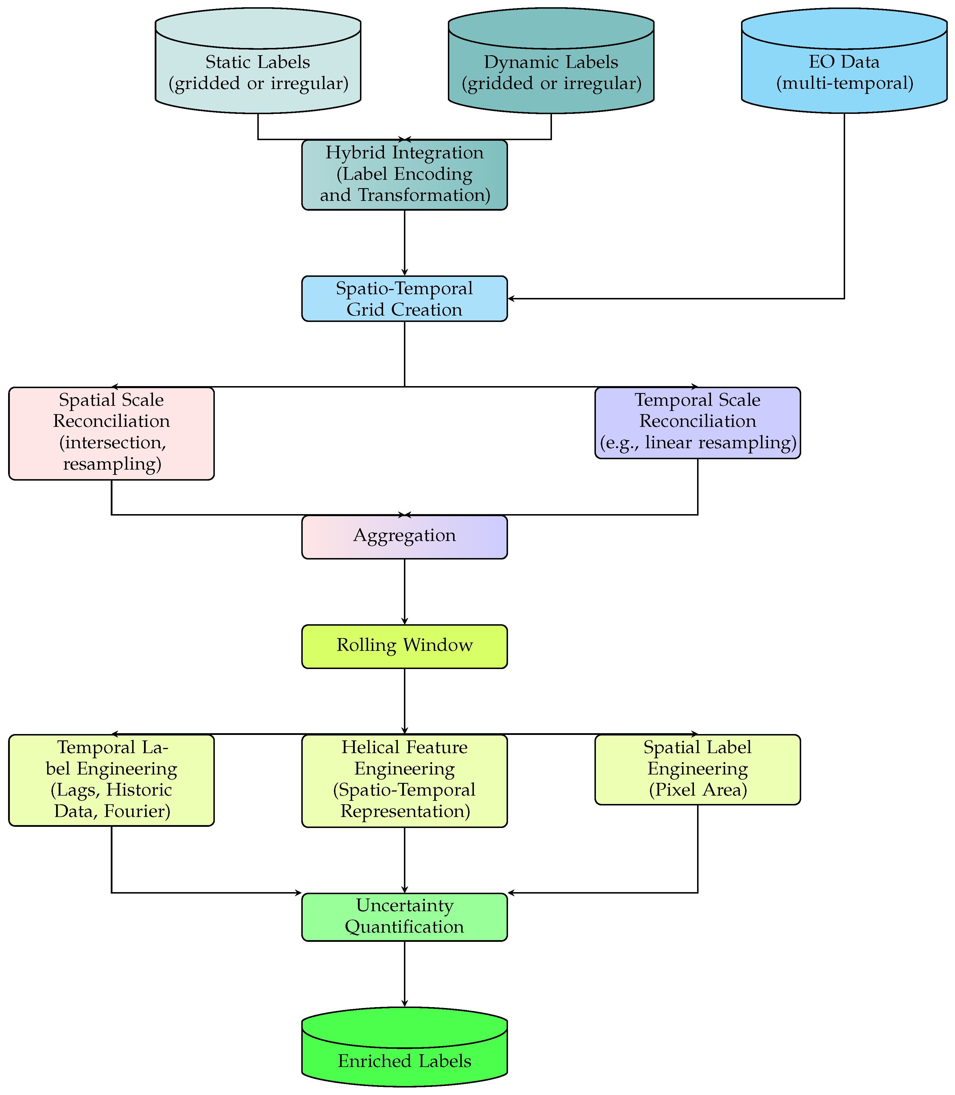
The HELIX framework in Figure 6 consists of multiple interlinked modules, each fulfilling a distinct purpose in the dynamic labelling workflow.

4.1.1. Hybrid Integration of Static and Dynamic Labels

The HELIX framework integrates various label sources into a unified hybrid dataset, irrespective of their original formats, including irregular vector data, gridded raster data, and georeferenced structured datasets (e.g., CSV). This integration effectively harnesses the complementary strengths of both temporally static data (e.g., soil maps, historical land use data) that provide stable long-term baseline conditions and temporally dynamic data (e.g., climate variables, vegetation indices) that capture environmental changes over time. The combination of diverse datasets regardless of their temporal characteristics (static or dynamic) or data types (numerical, categorical) is highly advantageous for training robust models in ML, DL, AI, and FM contexts. The HELIX framework automatically manages different data types, transparently encoding categorical labels into numerical forms to ensure traceability and reproducibility. By preprocessing all these diverse datasets within a single coherent pipeline, HELIX simplifies data handling, enhances model training efficiency, and maintains consistent label quality. This hybrid integration approach also adaptively addresses temporal variability, dynamically selecting between stable representations for persistent landscape features and dynamic representations for capturing short-term environmental fluctuations. 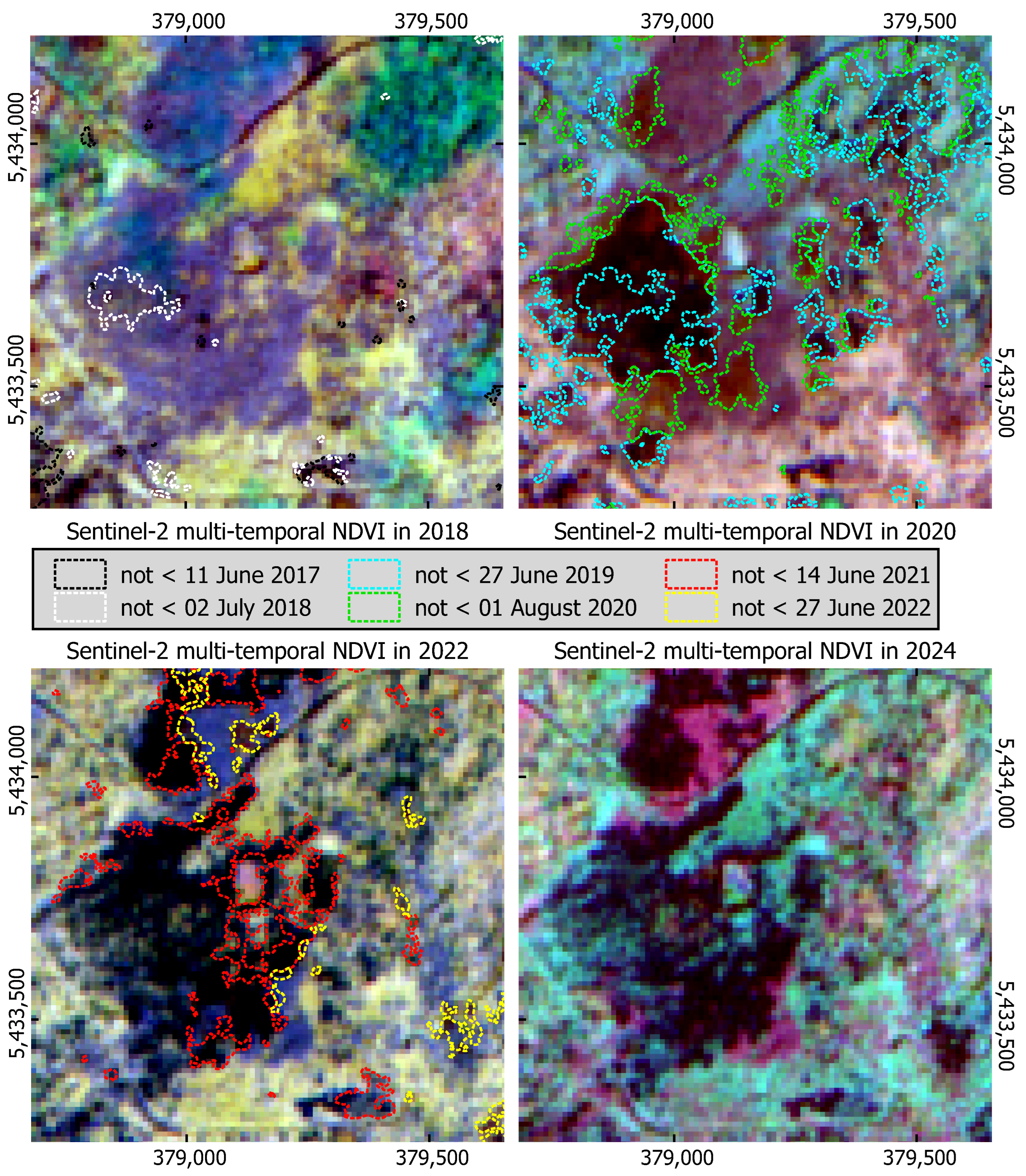For instance, Figure 5 illustrates scenarios where manually annotated static labels lag behind the frequently updated dynamic labels derived from Sentinel-2 NDVI data. Similarly, Figure 2 underscores the necessity of dynamic labels for accurately representing rapidly changing environments such as tidal zones.

4.1.2. Spatiotemporal Scale Reconciliation

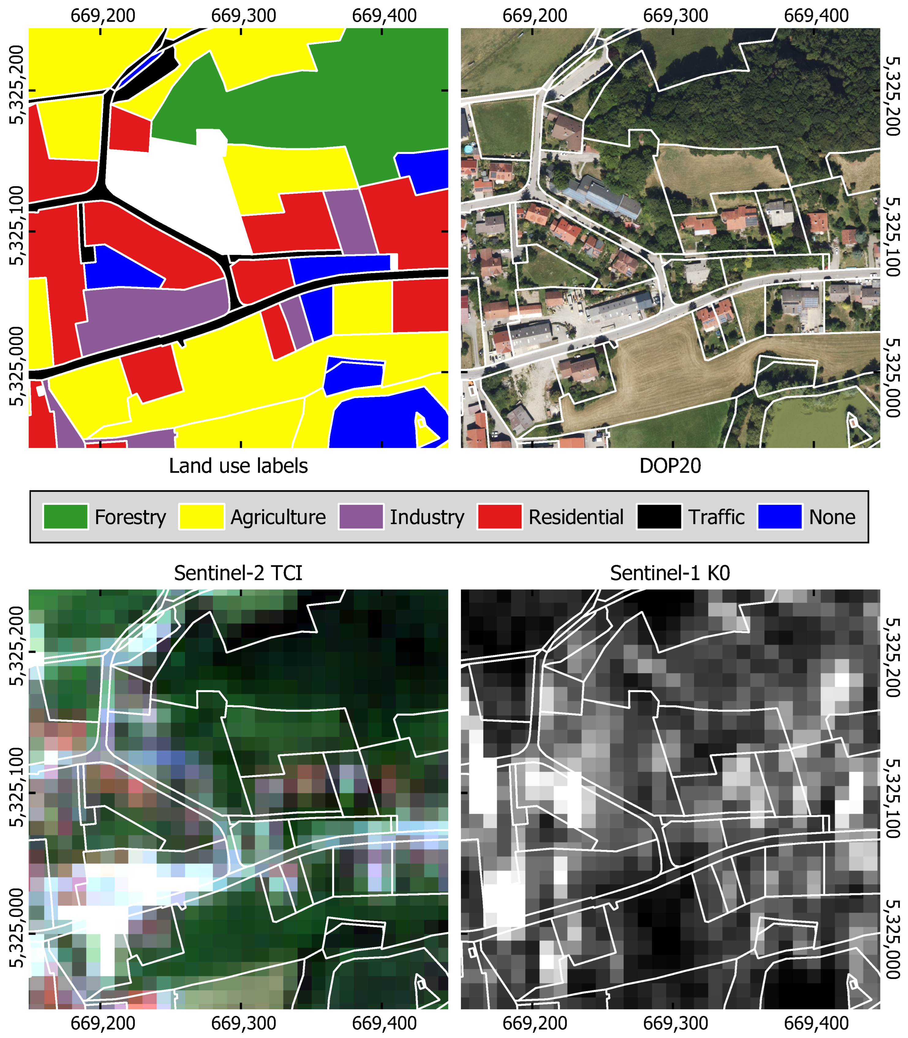
Many EO datasets and vector-based reference sources inherently exhibit misalignment across both spatial and temporal domains, complicating their direct integration into ML and DL models, AI-driven geospatial analytics, and FMs. The HELIX framework explicitly addresses these misalignments by systematically reconciling discrepancies between the reference labels, regardless of whether they are static, dynamic, or a combination of both, and the EO-derived features (e.g., satellite imagery). Practically, this is achieved by first extracting a reference grid, including coordinate reference systems (CRS), from the EO data, then identifying relevant temporal intervals corresponding to EO data availability. Spatial reconciliation involves precisely aligning vector-based labels to a defined EO raster grid using geometric alignment methods, such as affine transformations combined with appropriate resampling methods (e.g., nearest neighbour, bilinear interpolation). Temporal alignment is achieved through linear interpolation and resampling techniques, aligning the label timestamps precisely with those of the EO-derived features. This dual spatial and temporal reconciliation step enhances label quality, consistency, and adaptability, making it suitable for a wide range of model types. For example, Figure 1 illustrates spatial misalignment issues where detailed terrestrial labels require spatial resampling to match coarse satellite grids. Similarly, Figure 2 highlights temporal discrepancies arising from rapid tidal fluctuations, demonstrating the necessity of temporal alignment techniques provided by the HELIX framework.

4.1.3. Spatiotemporal Label Enrichment and Engineering

The HELIX framework further enhances label quality by leveraging sophisticated spatiotemporal enrichment techniques, providing significantly enriched reference datasets tailored for robust model training. Utilizing spatial and temporal dimensions simultaneously, the HELIX calculates additional derived features, including probabilities of specific classes or labels within defined spatial grid cells. For instance, it enables the calculation of label probabilities, such as the fractional area occupied by a particular class within each raster grid cell, thereby improving the interpretability and robustness of training labels.

Central to this enrichment is the configurable spatiotemporal windowing technique, in which both spatial extent (e.g., neighbourhood radius) and temporal duration (e.g., number of previous or subsequent time steps) are fully user-definable. This flexibility allows users to comprehensively integrate local context from spatially neighbouring pixels or polygons and temporal context from historical observations such as past land-use changes, trends, or seasonal cycles. Utilizing these configurable windows, the HELIX enables computation of novel and contextually rich features capturing the dynamic interplay between labels across space and time. Specifically, the HELIX supports the following processing steps:

• Spatial Aggregation: Calculation of neighbourhood statistics (mean, median, mode) to ensure consistency when integrating high-resolution vector labels with lower-resolution EO raster grids, as demonstrated in Figure 3 and Figure 4.
• Temporal Windowing: Employing rolling or sliding windows that capture short-term and long-term temporal dependencies, allowing for the detection and analysis of changes and trends over defined periods. The temporal window size and spacing are user-configurable.

By explicitly considering label interactions within these spatiotemporal windows, HELIX can effectively derive a comprehensive set of enriched features, significantly enhancing the representational fidelity of dynamic labels. Advanced scenarios such as tracking the progressive spread of bark beetle infestations (Figure 5) or monitoring overlapping windthrow areas can particularly benefit from HELIX’s robust spatiotemporal enrichment capabilities, significantly improving ML and DL model accuracy and generalization.

Temporal label enrichment within the HELIX framework is performed by systematically incorporating several complementary techniques. Lagged labels integrate past reference data values such as historical land-use records or previous environmental events, enabling models to capture and learn from long-term dependencies and temporal transitions. Seasonal label enrichment identifies recurring label patterns over defined periods, such as annual wildfire occurrences or periodic fluctuations in water levels, allowing for effective incorporation of cyclical dynamics into the training process. Furthermore, Fourier-based label refinement decomposes time series labels into dominant periodic components, explicitly modelling and capturing cyclic environmental trends such as phenological cycles. The unique Helical Label Representation (HLR) employed by the HELIX framework further enriches labels by aggregating spatial and temporal neighbouring labels simultaneously. This approach is particularly advantageous for accurately modelling environmental phenomena characterised by gradual and spatially progressive changes, such as pest infestations spreading or forest degradation evolving over time. Additionally, the integration of historical data layers to enhance temporal coherence and contextual depth. By combining archival shapefiles, previous EO-derived classifications, or historical survey data with contemporary observations, the framework effectively identifies and monitors persistent landscape transformations such as urban expansion or reforestation initiatives. This integration significantly refines temporal continuity, facilitating nuanced assessments of gradual environmental transitions rather than relying solely on abrupt categorical classifications.

A key advantage of the multi-source integration in HELIX is its inherent ability to validate and cross-verify label consistency across independent reference datasets. By systematically incorporating multi-source observations into the label generation process, the HELIX framework prevents reliance on a single dataset, thereby reducing potential biases. This multi-source validation step strengthens the label enrichment process in the following ways:

• Detecting and correcting inconsistencies by comparing generated labels against independent reference datasets.
• Cross-verifying time series labels to prevent anomalies from propagating into model training.
• Enhancing label credibility and reducing overfitting by ensuring that training datasets represent a diverse range of acquisition conditions.

By leveraging multiple sources, the HELIX framework proactively validates labels prior to probability estimation, ensuring consistency across spatial and temporal domains while preserving contextual accuracy.

4.1.4. Probability Estimation, Refinement, and Soft Thresholding

The HELIX framework employs probabilistic modelling techniques to refine label assignments in order to explicitly quantify uncertainties resulting from sensor inaccuracies, mixed pixels, and ambiguities in classification. Using a grid-based probability estimation approach, HELIX evaluates the reliability and correctness of each label by computing class probabilities within each spatial grid cell. Confidence-weighted annotations derived from these probabilistic assessments improve the robustness and interpretability of labels, especially in areas with ambiguous boundaries or gradual class transitions.

Soft thresholding is a core component of the HELIX’s adaptive approach, dynamically adjusting classification boundaries based on probabilistic outputs rather than fixed categorical thresholds. Practically, this means that the framework can reorganize previously rigid classification boundaries spatially and temporally, then adapt them based on observed environmental changes or variability. For instance, areas initially classified definitively can be reclassified or refined over time if probabilistic assessments suggest shifting ecological conditions such as vegetation encroachment, progressive land cover transitions, or incremental forest degradation. This dynamic adjustment allows HELIX to represent the real-world complexity of environmental phenomena more accurately and flexibly.

The resulting output from the HELIX framework is typically a multilayer raster dataset in which each band represents a different enriched or probabilistic labels that are readily compatible with standard ML/DL workflows. These outputs facilitate comprehensive analyses by providing detailed insights into the spatial distribution and temporal dynamics of labels, ensuring accurate representation and enhanced predictive performance. Recognizing the computational intensity of large-scale multi-temporal EO datasets, the HELIX framework leverages parallel and distributed computing infrastructure. It optimizes data storage, retrieval, and processing workflows, enabling efficient preprocessing of extensive geographic areas and lengthy temporal sequences without compromising accuracy or temporal resolution. The HELIX framework ensures temporal consistency, refines label representation, accounts for uncertainties, and efficiently scales across diverse geospatial contexts. By harmonizing static and dynamic data sources, it significantly enhances the reliability of reference labels, providing robust foundations for ML, DL, AI, and FM models used in environmental monitoring and analysis.

A core strength of the HELIX framework lies in its comprehensive and adaptive integration of static and dynamic reference datasets, which ensures accurate and contextually relevant labels across various temporal scales. The modular design allows users to tailor key preprocessing parameters such as spatial aggregation radii, sampling strategies, grid definitions, and temporal resolutions to the specific needs of their applications. Furthermore, the HELIX framework supports selective inclusion or exclusion of redundant information, optimizing label quality and reducing unnecessary data complexity. It substantially improves label quality through spatial aggregation methods, configurable temporal windowing techniques, and probabilistic label refinement. These enrichment strategies effectively mitigate inconsistencies and noise, enhancing the representational fidelity and contextual depth of the reference data. Additionally, the framework explicitly incorporates uncertainty quantification, offering probabilistic labels and confidence-weighted annotations, which significantly bolsters the robustness of a model predictions, particularly in ambiguous or noisy environments. Scalability is another notable strength, with the HELIX framework being specifically designed to leverage distributed and parallel computing architectures. This capability ensures efficient preprocessing of extensive datasets spanning large geographic areas and multiple temporal dimensions, making the framework highly suitable for operational EO applications.

Nevertheless, the HELIX framework does come with certain limitations. Its computational demands can be substantial, especially when handling high-resolution and extensive multi-temporal datasets, which potentially restricts its application in resource-constrained environments. Furthermore, the effectiveness of the HELIX framework heavily relies on the availability, quality, and representativeness of input data. This dependency could limit the framework’s effectiveness in regions where historical or dynamic reference datasets are sparse or of poor quality. Additionally, successful implementation and optimization of HELIX require considerable expertise in parameter tuning, selection of suitable spatiotemporal transformations, and careful interpretation of probabilistic outputs. While this manuscript focuses on presenting the conceptual schematic of the HELIX, a more detailed exploration of its algorithms, parametrization strategies, and real-world usability cases will be provided in future studies.

As HELIX continues to evolve, addressing class imbalances in reference labels remains a critical future direction. While current implementations effectively reconcile multi-source label inconsistencies, potential enhancements could incorporate techniques such as synthetic minority labelling, employing generative models, and data augmentation in order to strengthen representation of sparsely represented classes while maintaining spatiotemporal coherence. Class-aware spatial aggregation methods could also be developed to enhance the visibility of minority labels in order to prevent over-representation of dominant classes. Additionally, dynamic label reweighting using confidence-adjusted probabilities to manage the influence of labels based on rarity and spatial autocorrelation represents another promising area for advancement. These prospective enhancements offer scalable and practical solutions for improving label distributions, ultimately leading to more balanced training datasets. Furthermore, incorporating soft-thresholding classification techniques within the probabilistic refinement approach could dynamically address class imbalances, allowing for better detection and representation of rare but ecologically significant phenomena such as habitat shifts, early deforestation signals, and pest outbreaks. In this way, the HELIX framework can both improve label accuracy and ensure the ecological relevance and actionable insights in environmental monitoring and analysis.

4.2. Future Directions

Future research directions should not only address the challenges discussed in previous sections but also pioneer new approaches that integrate labels and EO-derived features in a unified framework. In current workflows, labels and EO data are often developed and processed separately, which may limit the overall performance and adaptability of ML and DL models. Future systems should enable joint optimizations of labels and features in which both the ground truth and EO measurements are iteratively refined and harmonized through other integrated preprocessing pipelines.

However, the independent validation of data is essential for ensuring the robustness and credibility of EO-based ML/DL models [85,86]. Regarding such methodologies, it is of utmost importance to implement safeguards that maintain statistical independence. Without such safeguards, label optimization risks being overly influenced by feature distributions, leading to biased models that lack external generalizability. Several approaches can help to mitigate these risks while allowing for improved label–feature consistency. One potential direction is the use of regularized loss functions [87] to enforce stability in label optimization. Loss function constraints can be designed to ensure that labels remain homogeneous across time and space, preventing abrupt shifts that may be artifacts of sensor inconsistencies rather than actual environmental changes. Multitask loss functions [88] could further help to balance label fidelity with other predictive objectives, allowing models to learn from additional supervision while maintaining independent label structures. Additionally, uncertainty-aware loss formulations [89] can be used to downweight highly uncertain labels, reducing the risk of unreliable training data distorting model predictions. In addition to loss function constraints, hybrid validation strategies offer another pathway to preserving independent validation while refining label-feature coherence [86]. Instead of allowing labels to be iteratively updated without external benchmarks, structured validation frameworks should incorporate holdout-based label validation, in which a subset of reference data remains untouched to act as an independent assessment benchmark. Similarly, domain-specific cross-validation approaches can be applied, ensuring that models are tested on geographically or temporally distinct regions rather than being evaluated solely within the training domain. Multi-source validation, in which generated labels are compared against alternative independent datasets such as ground truth surveys, crowdsourced data, or multi-sensor observations, can further help to prevent label optimization from reinforcing model biases.

Another promising avenue is the application of probabilistic [90] and Bayesian methods in label refinement. Unlike fixed categorical labels, probabilistic frameworks allow for the modelling of uncertainty in reference data, ensuring that transitions between classes or temporal variations are captured without forcing deterministic label assignments. Bayesian inference enables iterative label updates while incorporating independent prior knowledge, preventing labels from drifting toward overfitting feature distributions. Similarly, soft-labelling techniques [91] can assign probability distributions instead of discrete class assignments, allowing models to handle ambiguous or transitional regions (e.g., vegetation shifts, land cover change dynamics) with greater flexibility. Post hoc label calibration [92] offers another strategy for maintaining label independence while benefiting from refined representations. Residual label correction can help to detect systematic biases in label assignments after model training, ensuring that errors linked to specific geographic or environmental conditions do not propagate into future predictions. Additionally, contrastive label alignment techniques, in which labels generated under different modelling conditions are compared, can reveal inconsistencies that might otherwise go unnoticed. These methods are particularly useful in remote sensing applications where multiple sensors provide different perspectives on the same environmental variable, enabling a reconciliation process that respects external validation sources.

A further consideration for future research is the role of explainability and interpretability in label optimization [93]. As dynamically generated labels increasingly originate from prior ML/DL models rather than from direct human annotation, ensuring transparency in their construction is essential for scientific credibility in EO. In this context, feature explainability techniques that are typically used in feature engineering could also inform label engineering, particularly in cases where a prior model generates the reference data for subsequent learning processes. For instance, feature attribution methods such as Shapley Additive Explanations (SHAP) and Gradient-weighted Class Activation Mapping (Grad-CAM) can be used to assess whether label refinements capture meaningful geophysical signals rather than overfitting to latent model biases. Similarly, integrating Explainable AI (XAI) into label validation workflows could provide insights into whether dynamically optimized labels retain their conceptual and physical relevance, ensuring that feature-label dependencies remain interpretable and scientifically grounded.

Future research on label optimization must prioritize statistical independence and external validation as core principles. While integrating labels with EO-derived features offers potential advantages in model consistency, it is imperative that optimization strategies do not undermine the integrity of independent reference data. By employing a combination of loss function constraints, hybrid validation frameworks, probabilistic techniques, post hoc refinements, and explainable AI approaches, researchers can ensure that future labelling methods enhance model generalizability and maintain credibility in EO-based ML/DL applications. These advancements will be essential as automated dynamic labelling becomes more prevalent in large-scale geospatial modelling.

Currently, EO data is typically available in gridded format; however, an increasing amount of EO information is being captured as segmented high-definition data at fine scales (e.g., individual trees). Integrating such detailed EO data with corresponding labels is a pivotal future step in enhancing model performance and adaptability. Automated label verification involves the use of ensemble-based validation techniques to detect and correct inconsistent labels. By leveraging multiple model outputs and cross-validating with independent data sources, such techniques can significantly improve the quality and reliability of the reference data. This is crucial for ensuring that model training is based on accurate, consistent ground truth. The development of self-adapting labelling systems represents a promising research direction. Algorithms that dynamically adjust labels based on feedback from real-world observations can continuously refine the training data. Techniques such as self-supervised learning and domain adaptation are key to achieving this dynamic refinement over time. Such systems could both update labels in response to evolving environmental conditions and help in identifying and correcting systematic errors. A major future challenge is the current separation between label generation and EO data feature extraction. Future approaches should aim to integrate these processes into a single co-adaptive framework. By processing labels and EO data simultaneously in a unified pipeline, it would be possible to accomplish several goals:

• Enhanced data consistency: Joint processing would allow for simultaneous correction of spatial and temporal misalignments, ensuring that both labels and EO features are well-aligned.
• Improved label quality: Iterative refinement based on the combined insights from both data types could lead to more accurate and representative labels.
• Increased adaptability: A unified system could more readily adapt to changes in the environment, dynamically updating both labels and features in near real-time for future onboard processing.

Such an approach would represent a paradigm shift in which preprocessing not only prepares data for training but also continuously improves the quality of the reference data based on the EO observations. By tackling these challenges, dynamic labelling and joint data development can unlock the full potential of ML and DL in EO applications. Enhanced real-time environmental monitoring, improved land use prediction, and more effective disaster response capabilities are just a few of the potential benefits. The transition from static to dynamic labels and from separately processed labels and features to a joint development approach is not merely a technical evolution but a necessity for building more responsive and adaptable geospatial modelling systems. As strongly advocated for in previous studies, the future of EO data processing lies in creating robust, scalable, and integrated frameworks that not only address current challenges but also pave the way for more advanced and adaptive ML/DL applications in environmental monitoring. However, as emphasized by [48], the distinct nature of EO data necessitates frameworks that are tailored to its domain-specific complexities, including sensor characteristics, spatiotemporal dependencies, and physical data constraints. Unlike general computer vision applications, EO label engineering must integrate a deep understanding of remote sensing principles to ensure that dynamically generated labels remain scientifically valid and physically meaningful. Therefore, selecting analytical and geoprocessing frameworks for label optimization must prioritize EO-specific considerations in order to maintain the integrity and interpretability of reference labels.

5. Conclusions

Despite its fundamental impact on the reliability, accuracy, and generalizability of ML/DL/AI models, the role of reference data preprocessing in EO applications has long been underestimated. While advances in AI architectures have enhanced our ability to analyse complex spatiotemporal patterns, the quality and consistency of reference labels remain a major bottleneck. This review has demonstrated how static reference data alone are insufficient for capturing the evolving nature of EO datasets; instead, dynamic labelling strategies that address temporal variability, data heterogeneity, and label uncertainties are essential for developing adaptive and scalable AI/ML models in EO applications.

This review was motivated by several key challenges. Although EO data increasingly support AI/ML applications, issues such as temporal inconsistencies, missing data, and multi-source integration hinder effective analysis. While existing studies have proposed domain-specific solutions such as pixel-wise segmentation and time series classification, these methods often lack generalizability and scalability. Moreover, the field lacks standardized workflows for preprocessing dynamic reference data collected from such diverse sources as satellite, airborne, and UAV-based sensors. Without proper preprocessing, ML models risk learning biased or erroneous patterns that undermine reliable prediction.

Our analysis underscores the necessity of maintaining temporal consistency through alignment techniques that synchronize multi-source datasets and account for seasonal and long-term environmental changes. Spatial alignment methods such as resampling and neighbourhood-based aggregation are similarly important for mitigating discrepancies introduced by varying sensor resolutions. In addition, uncertainty management through probabilistic annotations and ensemble validation helps to quantify and correct errors in reference datasets. Scalability also remains a critical concern, as the growing volume and complexity of EO data demand efficient automated preprocessing workflows that can continuously update reference labels in near-real time.

Addressing these challenges requires a structured and adaptable approach. This article introduces the HELIX framework as one possible solution that meets the requirements identified by our extensive literature review. HELIX provides a systematic, scalable, and dynamic strategy for preprocessing spatiotemporal reference data. By integrating multi-source data harmonization, uncertainty quantification, and dynamic label updates, the HELIX framework represents a significant step towards standardizing EO reference data pipelines. Future research must now focus on operationalizing HELIX in practical implementations and ensuring its integration into diverse EO workflows.

Looking ahead, the transition from static to dynamic labelling represents not merely an incremental improvement but a fundamental shift in EO-driven ML. Future research must focus on developing standardized and scalable frameworks that integrate dynamic reference data with EO-derived features, ensuring interoperability and consistency across applications. The development of automated label verification systems and self-adapting labelling algorithms will also allow for further refinement of ground truth data, allowing models to remain responsive as environmental conditions evolve.

In summary, by embracing dynamic labelling methodologies and integrating best practices into preprocessing workflows, the EO community can significantly enhance the impact of ML and DL models. The future of AI in EO depends not only on sophisticated model architectures but also on the foundation of accurate, consistent, and temporally adaptive reference data. The methodologies and insights presented in this review offer a strategic roadmap for advancing EO applications, helping to transform remote sensing into a truly adaptive and predictive science.