Abstract
Spaceborne LiDAR systems are crucial for Earth observation but face hardware constraints, thus limiting resolution and data processing. We propose integrating compressed sensing and diffusion generative models to reconstruct high-resolution satellite LiDAR data within the Hyperheight Data Cube (HHDC) framework. Using a randomized illumination pattern in the imaging model, we achieve efficient sampling and compression, reducing the onboard computational load and optimizing data transmission. Diffusion models then reconstruct detailed HHDCs from sparse samples on Earth. To ensure reliability despite lossy compression, we analyze distortion metrics for derived products like Digital Terrain and Canopy Height Models and evaluate the 3D reconstruction accuracy in waveform space. We identify image quality assessment metrics—ADD_GSIM, DSS, HaarPSI, PSIM, SSIM4, CVSSI, MCSD, and MDSI—that strongly correlate with subjective quality in reconstructed forest landscapes. This work advances high-resolution Earth observation by combining efficient data handling with insights into LiDAR imaging fidelity.
1. Introduction
Spaceborne LiDAR systems have become indispensable tools for Earth observation, providing critical data on forest structures, glacier dynamics, and natural hazards [1,2,3]. They enable scientists to study environmental changes and processes with unprecedented detail, contributing significantly to our understanding of ecological systems. However, the current satellite LiDAR platforms, such as NASA’s GEDI [4] and ICESat-2 [5], face resolution constraints due to operational limitations like footprint size, photon acquisition rates, and onboard processing capacities. In contrast, airborne LiDAR systems like NASA’s G-LiHT [6] produce high-resolution data but lack the global coverage and scalability required for comprehensive Earth observation. Bridging the resolution gap between satellite and airborne LiDAR systems could significantly advance remote sensing applications across multiple scientific domains.
A promising approach to address these challenges involves the use of Hyperheight Data Cubes (HHDCs), which provide a novel representation of LiDAR data that captures the three-dimensional structural information of landscapes [7]. HHDCs are constructed by aggregating LiDAR returns into a three-dimensional tensor, with the dimensions representing spatial coordinates and height, effectively capturing the vertical distribution of features such as vegetation and terrain elevations. This rich representation not only facilitates advanced analyses of ecological structures but also works seamlessly with previous approaches by delivering traditional data products, such as Canopy Height Models (CHMs), Digital Terrain Models (DTMs), and Canopy Height Profiles (CHPs). By enabling the extraction of these conventional products within a unified framework, HHDCs ensure compatibility with existing methodologies while enhancing the potential for new insights. Moreover, HHDCs support advanced processing techniques, including footprint completion and super-resolution using Generative Adversarial Networks (GANs) [8] and diffusion models [9]. These methods can reconstruct missing or sparse data within HHDCs, improving the quality and resolution of the datasets. Additionally, by integrating HHDCs with other data modalities, such as hyperspectral images, it is possible to optimize terrain sampling strategies and enhance the accuracy of ecological representations [10,11]. This multi-modal integration supports applications like biomass estimation, canopy height modeling, and biodiversity assessment, which are critical for understanding and managing natural resources.
While HHDCs offer significant advantages in capturing and analyzing 3D ecological data, their implementation on spaceborne platforms introduces a critical challenge: efficiently processing and transmitting large data volumes under hardware constraints. This necessitates advanced compression methods to simplify 3D HHDC representations for efficient transmission to Earth, where extensive computational resources are available. Traditional compressed sensing (CS) approaches in remote sensing, such as those explored in NASA’s CASALS program and implemented in compressive satellite LiDARs (CS-LiDARs), often rely on structured or adaptive sampling strategies, including coded illumination and wavelength scanning, to reduce data volume while preserving scene information [7,10,12]. In contrast, our framework introduces a novel forward imaging model incorporating randomized illumination patterns, simplifying onboard hardware implementation by eliminating the need for adaptive designs or prior scene knowledge [13]. The randomization ensures essential compressed sensing properties, such as incoherence and efficient sampling [14,15], intuitively analogous to casting a net with randomly placed holes that captures representative scene information. Unlike recent diffusion model applications in remote sensing, which focus predominantly on image synthesis and optical imagery super-resolution [16,17], our approach uniquely integrates diffusion generative models with compressed sensing to reconstruct high-resolution 3D LiDAR data cubes from sparse measurements. To the best of our knowledge, this combination for satellite LiDAR data processing is unprecedented, offering a scalable solution balancing efficient data acquisition with high-fidelity reconstruction and providing rigorous evaluation metrics to ensure the reliability of ecological products derived from HHDCs [9,13].
In our framework, diffusion models enable lossy compression of HHDCs by generating compact representations optimized for transmission, which are then reconstructed into high-resolution 3D data on Earth. Diffusion models excel at learning complex data distributions and iteratively refining signal representations by progressively adding and removing noise [18,19]. Unlike traditional super-resolution applications, our methodology employs diffusion models within the HHDC framework to generate compressed representations that are optimized for efficient transmission and high-quality reconstruction on Earth. Moreover, integrating HHDCs with GANs and diffusion models enhances our ability to perform footprint completion and recover fine-grained ecological details [9].
Although the compression is inherently lossy, it provides a scalable solution for Earth observation. The reconstructed data, however, inevitably deviate from the ground truth, necessitating a detailed analysis of these distortions to ensure the reliability of LiDAR-derived products. By combining HHDCs with other representations, such as hyperspectral images, we can further optimize the sampling strategies and improve the accuracy of the reconstructed terrain models [10].
A key contribution of this paper is the rigorous evaluation of distortion metrics for LiDAR-based imagery and derived products within the HHDC framework. We analyze how the diffusion-based compression process impacts the data products used in ecological studies, including DTMs, CHMs, and percentile-based height measurements extracted from HHDCs. Additionally, we assess distortions in 3D reconstructions by evaluating them in waveform space, providing insights into how the compression algorithm influences spatial accuracy.
The primary contributions of this paper are as follows:
- We introduce a randomized illumination pattern within a modified forward imaging model, ensuring efficient sampling and enabling data compression for spaceborne LiDAR systems through the principles of compressed sensing, all within the HHDC framework.
- We propose a diffusion-model-based approach for lossy 3D HHDC data compression, facilitating high-resolution ground-based reconstructions while optimizing data for transmission.
- We perform an in-depth analysis of distortion metrics, evaluating the impact of diffusion-based compression on HHDC-derived data products, including DTMs, CHMs, and 3D reconstructions in waveform space.
By integrating randomized illumination patterns, compressed sensing principles, and diffusion-based reconstruction within the HHDC representation, our methodology offers a scalable and reliable solution for high-resolution Earth observation. Our work addresses the dual challenges of efficient data handling and distortion analysis, contributing to the development of next-generation satellite LiDAR systems that are capable of delivering detailed ecological and topological insights on a global scale.
The remainder of this paper is organized as follows. In Section 2, we introduce the Hyperheight Data Cube (HHDC), elaborating on its structure and benefits for representing complex ecological landscapes. Section 3 presents our Bayesian super-resolution approach, detailing the forward imaging model enhanced with a randomized illumination pattern for efficient data fidelity within HHDCs and the incorporation of diffusion models for regularization. In Section 4, we address the inverse problem arising in satellite LiDAR systems and describe how it can be solved through iterative posterior sampling guided by diffusion models within the HHDC framework. Section 5 provides an initial evaluation of various full-reference image quality assessment (IQA) metrics to determine their suitability for assessing the quality of reconstructed HHDC data. Building upon this, Section 6 offers a comprehensive analysis of the selected IQA metrics applied to our reconstructed HHDCs, including a dataset description, training and evaluation processes, and the evaluation of IQA metrics for sparse sampling and reconstruction. Finally, in Section 7, we conclude the paper by summarizing our findings and suggesting directions for future research.
2. Hyperheight Data Cube Representation
A Hyperheight Data Cube (HHDC) is a novel method for representing LiDAR data, specifically designed to capture the 3D structural information of landscapes. This approach is particularly useful for ecological studies, such as forest canopy profiling and digital terrain modeling. Unlike traditional 2D LiDAR profiles, which provide only a cross-sectional view along a satellite’s path, HHDCs capture a full volumetric data cube, encoding the length, width, and height of the observed area [7]. This 3D structure allows researchers to analyze detailed spatial information, making it highly valuable for studying vegetation and terrain and for applying advanced deep learning techniques. To understand how an HHDC is constructed, consider the point cloud shown in Figure 1a. This point cloud is accompanied by a cylindrical structure with a diameter equivalent to the size of the footprint of a satellite LiDAR shot. By analyzing the vertical distribution of the LiDAR returns within this footprint, we generate a waveform that resembles the elevation histogram typical of waveform LiDAR measurements, as presented in Figure 1b. By synthesizing similar LiDAR shots both in along-swath and across-swath directions and consolidating them into a single data tensor, we form the HHDC, illustrated in Figure 1c. The HHDC organizes LiDAR data into a 3D tensor, where the first two dimensions represent the spatial arrangement of laser footprints along and across the swath, while the third dimension captures the vertical structure of the scene, such as canopy height and terrain elevation. This format enables the extraction of biological features, including Canopy Height Models (CHMs), Digital Surface Models (DSMs), and Digital Elevation Models (DEMs). An voxel of the HHDC represents the number of photons found in the spatial location and at height, where is the vertical resolution. The 2D DTM, for instance, is created as the horizontal slice of the HHDC at the 2% percentile, as shown in Figure 2c, where the “bare Earth” landscape is clearly seen. The 2D CHM is shown in Figure 2a and computed as the 98% minus the DTM plane. Figure 2b shows the 50% that is typically used for biomass studies. As with many signals found in nature, HHDCs present a sparse representation. For instance, 3D wavelet representations of HHDCs of forests and vegetation in Maine show that less than of the wavelet coefficients are needed to accurately represent the HHDC. This property avails the opportunity to design compressive sensing protocols capable of capturing the essential information content in HHDCs with just a small number of compressive measurements.
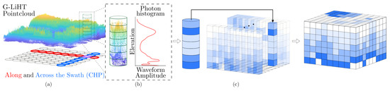
Figure 1.
The HHDC: (a) a tube-shaped illuminated footprint; (b) histogram of heights within the footprint; (c) concatenated height histograms building the 3D HHDC.
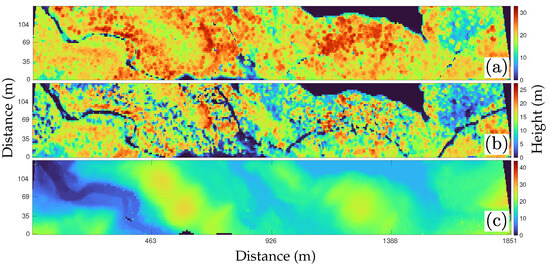
Figure 2.
(a) CHM of the HHDC. (b) 50% percentile as it is typically used for biomass studies. (c) DTM of the HHDC.
3. Bayesian Super-Resolution Framework: Forward Imaging Model and Diffusion Regularization
Satellite LiDAR systems often face limitations in spatial resolution due to constraints in photon density and footprint size. Super-resolution techniques address these limitations by reconstructing a high-resolution representation from sparse low-resolution measurements, thus enhancing spatial detail in LiDAR imaging. This provides a denser and more informative 3D representation that supports detailed environmental analysis. The objective of super-resolution is to recover a high-resolution HHDC, , from sparse measurements represented by a low-resolution HHDC, , where , , and . This problem is inherently challenging due to its ill-posed nature: multiple high-resolution representations can map to the same low-resolution measurements. Ref. [13] formalizes super-resolution within a Bayesian compressed sensing approach, defining a joint probability distribution over both the low-resolution measurements and the high-resolution tensor we aim to recover. Specifically, we consider the joint distribution , where the goal is to infer the high-resolution tensor, , given the observed low-resolution measurements, . By factorizing this joint distribution, we obtain
where represents the likelihood of observing the low-resolution measurements given a high-resolution representation, describing the distribution governing the LiDAR sensing process. is the prior over the high-resolution tensor, which encodes prior assumptions about the spatial structure of the high-resolution data. To recover , we maximize the posterior distribution , which can be expressed as
Since is independent of , maximizing the logarithm of the posterior simplifies to maximizing the joint likelihood and prior terms. Thus, Ref. [13] formulates the super-resolution task as the following optimization problem:
where is the data fidelity term, derived from the likelihood and represented by the Kullback–Leibler divergence between the observed measurements and the predicted measurements . Here, denotes the forward imaging model of the satellite LiDAR, enhanced with a randomized illumination pattern . The illumination pattern plays a crucial role in enabling a compressed representation of the high-resolution HHDC. Instead of targeting specific regions, introduces random variations into the illumination process. This randomness ensures the incoherence property that is essential for compressed sensing, which allows the system to efficiently capture and reconstruct the necessary information from fewer measurements. By spreading the measurement energy uniformly across the data space, we preserve essential details without requiring a dense sampling of the entire scene. This approach not only reduces the volume of data needed for accurate reconstruction but also simplifies the design and operation of the illumination system. Consequently, incorporating into the forward model aligns our methodology with compressed sensing principles, facilitating efficient recovery of (as discussed further in Section 3.1 and Section 4).
The term serves as a regularization term, integrating prior knowledge to encourage plausible high-resolution structures (detailed in Section 3.2). By combining the data fidelity term and the regularization term, the optimization process effectively reconstructs while balancing adherence to observed data and the incorporation of prior information.
3.1. Forward Imaging Model for Data Fidelity
The data fidelity term is computed using a forward imaging model, , which probabilistically describes the sensing process of the satellite LiDAR system. Given a high-resolution HHDC , the forward model outputs a distribution over low-resolution measurements, capturing the process that reduces spatial resolution through factors such as footprint size, Gaussian convolution, and photon loss. Formally, Ref. [13] models as being distributed according to where r represents the number of photons returning to the satellite per footprint and is a Gaussian kernel characterizing the footprint dimensions. To implement the forward model enhanced with an illumination pattern , it is necessary to capture three key phenomena in the LiDAR sensing process (as depicted in Figure 3):
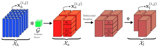
Figure 3.
High-resolution footprints, denoted as , within a high-resolution tensor , are convolved with a Gaussian kernel to produce aggregated footprints , encapsulated in the aggregated tensor . By applying multinomial sampling to each aggregated footprint, based on the photon count r, and selecting a random set of footprints, we derive low-resolution footprints , represented within the low-resolution tensor .
- Gaussian Beam Convolution: In satellite LiDAR, the laser shots exhibit a Gaussian beam pattern, which defines the footprint on the ground. This footprint’s energy distribution is modeled by a Gaussian convolution with the high-resolution data. The Gaussian kernel is defined by its Full Width at Half Maximum (FWHM) and the footprint radius at which the intensity drops to . The 2D Gaussian filter used to model footprint aggregation is expressed aswhere i and j are the integer indices of the kernel, k is its size, and . This convolutional operation aggregates neighboring high-resolution footprints, reducing spatial resolution while capturing the Gaussian spread of each footprint.
- Photon Loss with Distance—Multinomial Distribution: As the distance between the satellite and the ground increases, the number of photons returning to the detector decreases, leading to a reduction in photon count within each footprint. This phenomenon is modeled by a multinomial distribution, where the number of detected photons r in each footprint is distributed based on the energy received from each altitude bin. Given a high-resolution footprint histogram, the low-resolution photon counts are obtained by sampling from a multinomial distribution:where is the photon count in each bin, is the normalized probability for each bin, and c is the number of vertical bins. This model captures the stochastic nature of photon loss with increasing satellite altitude, reflecting the distribution of detected photons in low-resolution measurements.
- Illumination Pattern: To enhance data compression and ensure incoherence, an illumination pattern is incorporated into the forward model . The pattern represents a randomized selection of low-resolution footprints, distributing the illumination energy in a manner consistent with principles from compressed sensing. This randomization ensures that the measurements exhibit incoherence, a key property for accurate recovery in under-sampled systems. Unlike explicitly selective approaches, this randomized strategy simplifies the implementation while still preserving critical information required for reconstructing high-resolution structures within . By applying , the model achieves effective compression by capturing essential data elements without the need for a fully dense or adaptively designed sampling strategy, thereby reducing the overall data volume while maintaining reconstruction fidelity.
Together, these processes define , allowing us to compute the data fidelity term .
To incorporate the illumination pattern into the forward model , we implement as a randomized binary mask applied to the low-resolution footprint grid. Each element in is independently set to 1 with probability p (e.g., ), indicating that the corresponding footprint is illuminated and measured, and to 0 otherwise. This random selection of footprints ensures that the measurements are incoherent with the sparse representation of the high-resolution HHDC in some domain (e.g., Fourier or wavelet), a critical requirement for compressed sensing. By distributing the sampling randomly across the scene, captures a diverse set of measurements that enable accurate reconstruction of from fewer data points. This approach simplifies the onboard implementation compared to adaptive sampling strategies, which may demand complex hardware or prior scene knowledge, while still providing the necessary mathematical guarantees for recovery.
The use of a randomized illumination pattern is grounded in the principles of compressed sensing, where random sampling ensures incoherence with the sparse basis (e.g., wavelets) of the HHDC, enabling accurate reconstruction from a reduced number of measurements. This randomness satisfies the restricted isometry property (RIP) with high probability, providing universal recovery guarantees for any sparse signal without requiring prior knowledge of its sparsity pattern. In contrast, adaptive or optimized sampling strategies tailor the illumination to specific signal characteristics, potentially reducing the number of measurements further (e.g., by 20–50% for highly structured scenes, based on prior studies like [14]), but at the cost of increased complexity. For satellite LiDAR, where robustness across diverse unknown terrains and hardware simplicity are paramount, the randomized approach offers consistent performance without the need for real-time adaptation or sophisticated onboard processing. While adaptive methods might lower sampling rates for specific scenes, the randomized pattern’s simplicity and universality make it well suited for global Earth observation under operational constraints.
3.2. Diffusion Models for Regularization
To enforce the regularization term −, we employ diffusion generative models [18,19,20]. This formulation not only provides a powerful probabilistic prior for high-resolution HHDCs but also constrains the solution space of our compressed sensing problem, allowing the optimization algorithm to sample exclusively from the distribution of high-resolution data learned by the diffusion model. The SDE-based diffusion model consists of two main processes (as depicted in Figure 4): a forward diffusion process that progressively corrupts data by adding noise and a reverse diffusion process that undoes this noise, ultimately sampling from a distribution that closely matches the high-resolution data. The SDE framework offers continuous control over noise injection and removal, making it highly suitable for guiding the compressed sensing optimization.
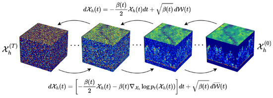
Figure 4.
Denoising diffusion methodology. Starting from a tensor of pure noise , the system learns to reconstruct the high-resolution HHDC by following a series of learned denoising steps described by the score function .
3.2.1. Forward Diffusion Process
The forward diffusion process (Figure 4-top) is modeled as a stochastic differential equation (SDE) that gradually transforms a clean high-resolution tensor into pure noise over continuous time . Ref. [19] represents this process as
where is the drift term, governing deterministic changes in over time t, is the diffusion coefficient that scales the noise added at each instant, and is an increment of a Wiener process. In the variance-preserving (VP) framework [19], we set the drift term as where is the noise schedule that controls the rate of variance addition over time. This drift term pulls toward zero, effectively centering the distribution of as noise increases. The diffusion coefficient , which scales the noise, is given by The schedule is typically chosen as an increasing function of t, ensuring that the injected noise grows over time. Common choices for include linear and cosine schedules, both of which enable a smooth transition from structured data to pure Gaussian noise. At , we begin with a sample drawn from the high-resolution data distribution . As t approaches T, converges to a known prior noise distribution, forming a flexible and stable framework for diffusion-based generative modeling. For the remainder of this paper, we adopt this variance-preserving (VP) approach, with the defined drift and diffusion terms, to control variance throughout the forward diffusion process. In our implementation, we employed a linear noise schedule for , where increases linearly from to over diffusion steps, consistent with the standard practice in Denoising Diffusion Probabilistic Models (DDPMs) [18], as will be described in Section 4.1. This schedule ensures a gradual increase in noise during the forward process, facilitating a smooth transition from the high-resolution HHDC distribution to a pure Gaussian noise distribution. We chose this linear schedule for its simplicity and proven effectiveness in generative modeling tasks, such as image generation, which shares similarities with our task of reconstructing detailed forest landscapes from sparse LiDAR measurements. The choice of steps balances computational efficiency with the ability to capture fine-grained details in the reverse diffusion process, while the range of values ensures that the model learns to denoise effectively across all stages of corruption.
3.2.2. Reverse Diffusion Process
To reconstruct high-resolution data from noise, we define a reverse-time stochastic differential equation (SDE) that progressively removes the noise added during the forward process (Figure 4-bottom). According to Anderson’s theorem [21], the reverse diffusion process, which generates samples from the high-resolution distribution, can be expressed as
where is the score function, representing the gradient of the log probability density of at time t. This term encourages the process to move in directions that increase the likelihood of high-resolution data, effectively constraining the solution to realistic high-resolution HHDC representations. is a Wiener process in reverse time, effectively “undoing” the stochastic increments of the forward process. This reverse SDE guides from pure Gaussian noise at back to a high-resolution sample at . By incorporating the score function , the model is able to infer the structure in high-resolution data, making it more likely to produce realistic samples. This gradient-based component, weighted by the schedule , effectively constrains the sampling process to lie within the distribution of high-resolution data while following the forward process’s variance-preserving setup. This combination of drift and score-guided diffusion provides a smooth and effective path back to high-resolution data.
4. Solving the Inverse Problem via Posterior Sampling
In the framework of satellite LiDAR super-resolution, solving the inverse problem is formulated as sampling from the posterior distribution , as defined in Equation (2). Leveraging the diffusion model in this process, we iteratively refine the high-resolution estimate by directing the reverse diffusion with the posterior score function, . This guidance enables the diffusion process to navigate toward configurations that are consistent with both the observed data and our prior knowledge. By Bayes’ rule, the posterior score can be decomposed as
where represents the score of the likelihood term. This term enforces data fidelity by aligning the reconstructed high-resolution data with the observed low-resolution measurements . Notably, this score is inherently linked to the KL divergence term in Equation (3), , where minimizing the KL divergence effectively maximizes the likelihood , ensuring that closely matches . The second term, , is the score of the prior distribution, encoding structural assumptions about that are enforced by the diffusion process. This term constrains the solution space, directing the optimization to sample from the high-resolution data distribution learned by the diffusion model. Combining both terms in the posterior score enables a high-resolution reconstruction that aligns with observed data while respecting the priors imposed by the diffusion process, ultimately finding the optima for Equation (3).
However, directly computing the likelihood term at each optimization step is computationally expensive as it requires a complete reverse diffusion process. Each step in this process involves multiple neural network evaluations to iteratively denoise the high-resolution tensor , which becomes prohibitive for real-time or large-scale applications. To mitigate this, Ref. [22] proposed Diffusion Posterior Sampling (DPS), which approximates the posterior using Tweedie’s formula [23]. This formula provides an estimate of the fully denoised HHDC based on the observed noisy sample, approximating the posterior mean without requiring a full denoising at each iteration. Specifically, for an intermediate noisy sample at time t, Tweedie’s formula estimates the clean fully denoised tensor as
where is a time-dependent scaling factor, and is the score function approximated by the pre-trained diffusion model. This estimate enables the posterior sampling process to bypass the costly neural network evaluations for a full reverse diffusion pass by using the denoised tensor to efficiently compute the likelihood term. Our key contribution modifies DPS to enhance its accuracy by replacing the original norm-based optimization with the gradient of the KL divergence term that uses an illumination pattern , achieving efficient posterior sampling guided by data fidelity and high-resolution priors. By iteratively applying this approximation, DPS with the KL divergence term efficiently samples from , reconstructing a high-resolution HHDC that is both consistent with the low-resolution sparsely sampled observations and constrained by learned high-resolution priors.
4.1. Algorithm Implementation
As described in Section 3.2.1, we adopt the variance-preserving (VP) framework for diffusion models. To implement this framework algorithmically, a discretized version of Equation (5) is required. For this purpose, we divide the time domain into N discrete bins and define , representing the state at the i-th time step. The noise schedule at the i-th step is denoted as . Following the framework of DDPM [18], we set , which represents the complementary noise weight. The cumulative product of noise weights up to the i-th step is given by . Additionally, we define , which plays a crucial role in characterizing the variance during the reverse diffusion process. This discretization forms the foundation for the numerical implementation of the diffusion process. With these definitions, we implement our modified version of DPS as outlined in Algorithm 1. The key modification—incorporating the illumination pattern into the KL divergence—is highlighted in purple, providing a clear distinction of our contributions.
| Algorithm 1 Diffusion Posterior Sampling [22] with KL divergence and illumination pattern. |
|
4.2. Need for Quality Assessment of Reconstructed Data
While our diffusion-based reconstruction algorithm demonstrates promising results in super-resolving HHDCs from sparse measurements (as will be shown in Section 6), it is imperative to evaluate the quality and reliability of the reconstructed data. The inherent lossy nature of the compression and reconstruction process can introduce deviations from the ground truth, potentially impacting downstream applications such as ecological modeling and biomass estimation. Therefore, a thorough analysis using image quality assessment (IQA) metrics is necessary to quantify the fidelity of the reconstructed HHDCs and ensure their suitability for practical use. In the following sections, we delve into the evaluation of various IQA metrics to assess their effectiveness in capturing the quality of reconstructed forest landscapes.
5. Evaluating Image Quality Metrics for Reconstructed LiDAR Data
Building upon the necessity to evaluate the reconstructed Hyperheight Data Cubes (HHDCs), we explore the suitability of existing image quality assessment (IQA) metrics for our application. IQA metrics play a vital role in quantifying the perceptual and structural fidelity of reconstructed images compared to the ground truth. In the context of LiDAR data and HHDCs, it is essential to identify metrics that accurately reflect the quality of the reconstructed 3D representations. This section presents a preliminary verification of various full-reference IQA metrics to determine their applicability and effectiveness in assessing the quality of forest landscapes reconstructed from compressed LiDAR data.
The task at hand, i.e., estimating the quality of forest landscapes reconstructed from LiDAR data, is relatively novel. Previous publications [11] on this topic have predominantly relied on metrics such as Mean Absolute Error (MAE), Mean Squared Error (MSE), and Structural Similarity (SSIM) [24] to characterize and compare the performance of various reconstruction techniques. However, these metrics may not be the most suitable for this specific application, and incorporating additional metrics of a different nature could prove beneficial. This assertion is supported by two main considerations. Firstly, MSE (or, equivalently, PSNR) is highly correlated with SSIM [25], making the simultaneous use of both metrics redundant. Secondly, while these metrics are still widely employed across many image processing applications, a significant number of newly proposed full-reference and no-reference visual quality metrics have demonstrated efficacy in alternative contexts [26], suggesting their potential utility in this domain.
Identifying efficient and adequate metrics for compressive sensing and related applications, such as sparse reconstruction, is of particular interest. Commonly used criteria include recovery success rate, reconstruction error, recovery time, compression ratio, and processing time [27]. However, in our case, recovery and processing time are not of primary concern. The work in [28] explores the use of no-reference metrics and introduces the CS Recovered Image Quality (CSRIQ) metric, which measures both local and global distortions in recovered data. Subjective assessments of restored image quality are thoroughly investigated across several databases in [29], where it is shown that the Codebook Representation for No-Reference Image Assessment (CORNIA) metric [30] performs well for sparse reconstruction. Additionally, Ref. [31] examines several full-reference quality metrics for image inpainting, noting that the most effective metrics, achieving Spearman’s rank-order correlation coefficient (SROCC) with Mean Opinion Score (MOS) values exceeding 0.9, are not widely adopted for characterizing other types of distortions.
Thus, we decided to conduct an initial analysis of existing metrics’ properties using the Tampere Image Database (TID2013) as it includes data for distortion #24—image reconstruction from sparse data [32]. This part of the database comprises 25 test images with five levels of distortion corresponding to PSNR values of approximately 33, 30, 27, 24, and 21 dB. Notably, PSNR = 33 dB corresponds to almost invisible distortions, also referred to as just-noticeable distortions (JND) [33], whereas PSNR = 21 dB represents distortions that are generally considered annoying. The other cases lie between these extremes.
Although the method of sparse reconstruction employed in TID2013 differs from that used for forest landscape reconstruction, which is highly specific, we believe that visual quality metrics based on the human visual system (HVS) can be valuable. These metrics account for features such as edge, detail, and texture preservation more effectively than PSNR or SSIM. This consideration is particularly relevant for forest landscapes, where sharp transitions and textures are common and must be preserved during the reconstruction process.
A good metric is expected to exhibit a high rank-order correlation with MOS, which represents the average subjective quality assessment from multiple participants. This assumption has been validated across numerous applications [34]. Consequently, higher Spearman’s rank-order correlation coefficient (SROCC) values serve as strong evidence for a metric’s suitability in specific applications (when calculated for images with certain distortion types) or its general applicability (when calculated across various distortion types in TID2013 or similar databases).
We calculated SROCC values for three groups of images:
- Images with sparse sampling only, to identify the most effective metrics for this case and lay the foundation for further analysis;
- Images with sparse reconstruction combined with additive white Gaussian noise, assuming noise may be present in our data;
- Images with sparse reconstruction and lossy compression, to evaluate metrics that perform well when data are compressed and subsequently reconstructed.
It is important to emphasize that the obtained results do not guarantee that the behavior of metrics in the context of our specific application will exactly match their performance on the color image database. Nevertheless, these findings provide a preliminary heuristic foundation for further investigation.
Recall that all distortion types in the TID2013 database are assigned dedicated indices. Table 1 lists the distortion types relevant to this study. We computed SROCC values for three groups of distortions as follows:

Table 1.
Distortions of interest in the TID2013 database.
- #24—to focus exclusively on sparse sampling distortions;
- #1 and #24—to compare the adequacy of sparse sampling distortions (type 24) with additive white Gaussian noise (type 1), which is the most commonly considered distortion type for quality metrics;
- #10, #11, #21, and #24—to jointly analyze sparse reconstruction and distortions arising from lossy compression.
It is worth noting that, for most visual quality metrics, higher values indicate better quality (e.g., PSNR or SSIM). However, some metrics are designed such that smaller values correspond to better quality. In these cases, SROCC is negative and should approach −1.
We evaluated 60 full-reference metrics, and the resulting SROCC values are presented in Table 2. Additionally, Pearson’s linear correlation coefficients (PLCCs) were computed for distortion type #24, as well as for two other groups of the TID2013 subsets mentioned above, using a nonlinear fitting function derived from the entire TID2013 dataset. This fitting approach, recommended by the Video Quality Experts Group (VQEG), is widely used in image quality assessment to account for the nonlinear characteristics of the human visual system (HVS).
Table 2.
The SROCC and PLCC values for the considered FR metrics for different groups of distortions. The top 10 results in each group according to absolute SROCC and PLCC values are ranked in brackets. The small letters g and y after the names of metrics denote the color-to-gray conversion using YUV and YCbCr color models, respectively.
Before starting data analysis, some preliminary comments are needed. In general, it is difficult to obtain SROCC larger than 0.98 due to the limited number of experiment participants and the diversity in their opinions. Hence, SROCC values equal to 0.97 or even 0.96 can be treated as excellent results. Then, the following conclusions can be drawn:
- there are numerous metrics that produce better results than PSNR and SSIM;
- the best of them are GMSD, MCSD, HaarPSI, PSIM, PSNR-HMA (description below), and some others for various subsets; we can decide what metrics to choose for further use;
- there are other factors that can influence the choice of appropriate metric; for example, most metrics analyzed above are suited for characterizing the visual quality of color images, but we have data arrays more similar to grayscale images; then, such metrics as PSNR-HMA can be replaced by PSNR-HVS-M;
- the metric’s computational efficiency is not important for the considered application since the metric is used for quality characterization but not in the image processing loop;
- usually, if a given visual quality metric shows that image/data quality is good, then the results of parameter estimation for such data are good as well;
- metrics have different ranges of their variation: some of them are expressed in dB, and others are in the limits from 0 to 1; because of this, it is necessary to consider these peculiarities in the analysis of data based on calculated metrics.
Most of the best metrics originate from the SSIM idea; however, they are calculated using additional image preprocessing and/or transforms. For example, Gradient Magnitude Similarity Deviation (GMSD) [37] utilizes global variation regarding gradient-based local quality maps, assuming the use of the Prewitt filter to determine the local gradient values. Then, the gradient similarity map is obtained using a formula similar to the SSIM calculation. The idea of Multiscale Contrast Similarity Deviation (MCSD) [38] is based on the calculation of contrast similarity deviations for three scales and further pooling using their weighted product. The contrast similarity between two compared images is also calculated using the SSIM-like formula. Both of these metrics are also characterized by relatively low computational complexity.
The Perceptual Similarity (PSIM) metric [35] extracts the gradient magnitude maps using the Prewitt filter, which are then compared using the multiscale similarity computation, further subject to perceptual pooling. As in the previously mentioned metrics, the similarity measure applied for the detection of differences between the gradient magnitude maps of the assessed image and the reference one is similar to the original SSIM formula.
Another computationally inexpensive metric, namely Haar wavelet-based Perceptual Similarity Index (HaarPSI) [44], is based on the wavelet decomposition conducted using six two-dimensional Haar filters. The coefficients obtained are compared to determine the local similarities and the importance of particular regions of the image. This metric takes into account such a feature of human vision as human attention or saliency, and this can be the reason why it is among the best. It should also be noted that most of the best metrics utilize gradient information in some way or another.
Nevertheless, the PSNR-HMA metric [36], also listed as one of the best metrics, has a different “nature” since it is a modification of the simple Peak Signal to Noise Ratio (PSNR) with additional use of Contrast Sensitivity Function (CSF) between-coefficient contrast masking of DCT basis functions, as well as mean shift and contrast changing.
6. Detailed Assessment of IQA Metrics on Reconstructed Hyperheight Data Cubes
Based on the preliminary verification of IQA metrics, we have identified several metrics that show promise in evaluating the quality of reconstructed HHDCs. In this section, we conduct a comprehensive analysis of these metrics in the specific context of our reconstructed LiDAR data. We apply the selected IQA metrics to our dataset of reconstructed HHDCs to assess their performance and correlation with subjective perceptions of quality. This analysis provides valuable insights into the most effective metrics for evaluating the fidelity of reconstructed forest landscapes and informs potential refinements in our reconstruction approach.
6.1. Dataset Description
For training and testing, we utilize data regarding the Smithsonian Environmental Research Center (SERC) in the state of Maryland (Latitude 38.88° N, Longitude 76.56° W). This dataset was derived from highly dense low-altitude point cloud measurements collected as part of the NSF’s National Ecological Observatory Network (NEON) project [75,76], providing a comprehensive representation of the region’s forested landscapes. A dataset of emulated HHDCs was created using high-resolution point clouds from the SERC region. The input low-resolution HHDC footprints were modeled with a uniform diameter of 10 m, spaced 3 m apart along the swath and 6 m across the swath, with a vertical resolution of 0.5 m (these values were chosen to match the LiDAR instrument currently under development as part of NASA’s CASALS project). These HHDCs were standardized to a fixed size of (footprints across the swath × footprints along the swath × height), corresponding to a forest tile covering m with a height of 64 m. For super-resolution to 3 m, the high-resolution output HHDC footprints were designed to increase the resolution while maintaining the same coverage area. Specifically, the footprints were assigned a radius of 3 m, with a 3 m separation both along and across the swath and a vertical resolution of 0.5 m. This configuration resulted in a tensor size of while preserving the original m area.
6.2. Training and Evaluation
The study demonstrates the effectiveness of compressed sensing using only 25% of the available footprints to reconstruct and super-resolve high-resolution 3D LiDAR data. Our approach achieves super-resolution from the native CASALS resolution down to a 3 m ground sampling distance. Figure 5 compares the performance of our diffusion-based model with that of a 3D convolutional autoencoder, while Figure 6 provides error maps indicating the strengths and weaknesses of the model in different views. To train the algorithm, approximately 12,000 data cubes were used, and data augmentation—random vertical and horizontal flips—was incorporated into the pipeline to enhance the model’s robustness. The system employs a standard U-Net architecture to learn the score function of the probability distribution, as is traditional in diffusion models. Training was conducted on an NVIDIA A100 GPU using a batch size of 64 for a total of 300,000 mini-batches. The diffusion-based approach produces reconstructions with a level of realism unmatched by other systems, capturing fine-grained details and subtle terrain variations. However, the model is prone to hallucinations, generating occasional artifacts not present in the original data. This highlights the need for further investigation to improve its reliability and ensure consistent performance across diverse environments. Despite these challenges, the diffusion-based model significantly outperforms the autoencoder, demonstrating superior realism and structural fidelity in the reconstructions. This underscores its potential as a robust tool for remote sensing applications, particularly in scenarios with limited sampling budgets. The system’s effectiveness, combined with the incorporation of data augmentation and efficient training on high-performance hardware, showcases its capability to handle large-scale LiDAR datasets while pushing the boundaries of compressed sensing and super-resolution methodologies.
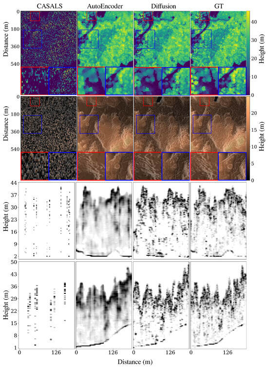
Figure 5.
Comparison of the proposed compressed sensing algorithm based on diffusion generative models with a traditional convolution 3D autoencoder used for inpainting. Going from top to bottom, we show CHM, DTM, a profile along track, and a profile across track.
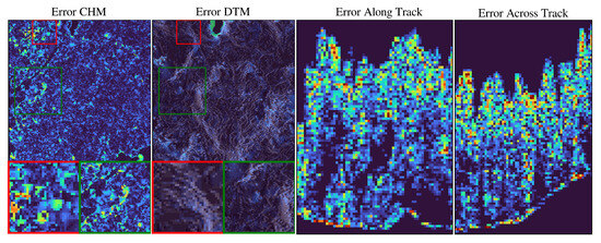
Figure 6.
Comparison of CHM, DTM, along track, and across track absolute errors for a forested area at the Smithsonian Environmental Research Center (SERC) using our diffusion approach to compressed sensing reconstruction using a random illumination pattern with 25% sampling ratio. Darker shades of blue indicate lower differences.
6.3. Evaluation of Image Quality Assessment Metrics for Sparse Sampling and Reconstruction
Building upon the promising results of the reconstruction process, we turn our attention to evaluating the quality of the generated high-resolution HHDCs using established image quality assessment (IQA) metrics. The reconstructed outputs were assessed against the original high-resolution data to measure the accuracy and structural fidelity of the super-resolution process. This analysis focuses on understanding how sparse sampling impacts reconstruction quality and the role of specific full-reference (FR) IQA metrics in capturing these effects. To ground this evaluation, we utilize data provided by the NSF’s National Ecological Observatory Network (NEON) for the SERC region. The insights gained from this evaluation allow us to identify which IQA metrics are most relevant to this application and how they can guide further improvements in reconstruction methodologies.
Using the approach described above, four experiments were conducted using different sizes of reconstructed areas defined by the lengths of square sides equal to 576 m, 288 m, 144 m, and 96 m. For each reconstructed area, five percentiles acquired from the canopy profiles were used in the analysis: 2nd (DTM), 25th, 50th, 75th, and 98th (CHM). The most relevant ones are the DTM, which illustrates the topography and relief of the terrain, and the CHM, which represents the height distributions of the trees. According to [7], using the 100th percentile is not recommended to avoid the influence of noise. Nevertheless, the middle percentiles may also be useful, e.g., for biomass studies. Finally, the obtained reconstructed data, being the correct outputs of the neural network, contain 60 HHDCs for 576 m, 354 HHDCs for 288 m, 782 HHDCs for 144 m, and 1231 for 96 m.
Since some of the IQA metrics used in Section 5 require color images as inputs and the obtained representations of the reconstructed HHDC profiles are matrices containing single numbers, they were preprocessed to make it possible to use them directly as input data treated as grayscale images. First, the values of high-resolution reference were multiplied by 2 to increase the data range and then such obtained values were replicated to three channels treated as RGB values by the metrics designed initially for color image quality assessment.
In some cases, the images representing high-resolution reference data and reconstructed images contain large regions of zero values; hence, not all metrics can be effectively used, resulting in incorrect output values. Therefore, some of them, including FSIM, WSNR, PSNR, RVSIM, and SFF, had to be removed from further experiments. Some other metrics included in Table 2, calculated for various color-to-gray conversion methods, were applied only once due to the use of the single-channel input data.
During each of the four experiments (for various area sizes), several IQA metrics were calculated using the reconstructed image and the high-resolution reference for the comparison. Since some of the reconstructions contained some errors, e.g., being the result of hallucinations of the neural network, it is expected that a “good metric” should be sensitive to them. Such a metric should also behave similarly for different sizes of images, and its universality should make it possible to apply it efficiently for various canopy profiles. Therefore, the similarity matrices were calculated, which illustrate Pearson’s correlations between the individual metrics’ results obtained for each of the five percentiles used in the experiments (2%, 25%, 50%, 75%, and 98%).
Considering the nature of the data, it is expected that the correlations between the results obtained for DTMs (2%) and CHMs (98%) should be the lowest ones, and the highest values should be obtained between the middle percentiles. Such correlation matrices were determined for each of the four sizes of the reconstructed areas. Sample results obtained for selected metrics are illustrated in Figure 7, where the diagonal values are obviously equal to 1, and the elements under the diagonal illustrate the correlations of IQA results obtained for two different percentiles.
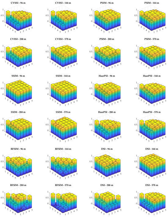
Figure 7.
Sample visualizations of the correlation matrices obtained for 5 profiles using various sizes of the reconstructed areas using six IQA metrics (CVSSI, PSIM, SSIM, HaarPSI, RFSIM, and DSI).
Analyzing the plots presented in Figure 7, results consistent with expectations can be observed for CVSSI and PSIM metrics, as well as for HaarPSI. It may also be observed that SSIM metric behaves differently for larger areas than for smaller ones where the inter-profile correlation of this metric’s values is much higher even for the highest (CHM) and the lowest (DTM) percentile. On the other hand, much less “stable behavior” may be easily noticed for RFSIM and DSI metrics.
To assess the behavior of these metrics numerically, the average correlation values between the pairs of these elements matrices were calculated. The final similarity was calculated as the average of six cross-correlations calculated for the following pairs of correlation matrices: 576 m to 288 m, 576 m to 144 m, 576 m to 96 m, 288 m to 144 m, 288 m to 96 m, and 144 m to 96 m. This way, a single value illustrating “the correlation of correlation matrices” was obtained, denoted as an average similarity. Additionally, similar calculations were conducted for the gradient matrices to demonstrate the similarity regarding changes in inter-profile correlations in four conducted experiments (for various sizes of the reconstructed area), denoted as average gradient similarity. The obtained results are presented, together with the illustration of the SROCC and PLCC values presented in Table 1 for distortion #24, in Figure 8.
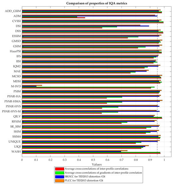
Figure 8.
Illustration of average cross-correlations of inter-profile correlations, the average cross-correlations of gradients of inter-profile correlations, and SROCC values for distortion #24, obtained for considered IQA metrics.
Analyzing the results presented in Figure 8, some IQA metrics may be distinguished as leading to “stable behavior” with a high correlation to the subjective perception of sparse sampling and reconstruction typical for remote sensing applications considered in the paper. Among the metrics combining such properties, the following ones should be noted: ADD_GSIM, CVSSI, DSS, GMSD, HaarPSI, MCSD, MDSI, PSIM, and SSIM4 since all values of the analyzed correlations and cross-correlations exceed 0.95. On the other hand, significantly worse results may be observed for UIQI, SSIM, or MAE, which were used in earlier papers.
The last step in analyzing the properties of the IQA metrics considered in our experiments was to verify their accordance with subjective quality evaluation. To illustrate the properties of the selected metrics, five sample high-resolution and reconstructed images are presented in Figure 9, together with the selected metrics’ values. The best subjective quality of the reconstructed image was reached for the first image with a visible river. Undoubtedly, the worst subjective quality was obtained for the reconstruction of the last image. Therefore, the values of metrics should reflect this. Nevertheless, well-known metrics such as MAE or SSIM demonstrated different results as similar values were obtained for the last of the images presented in Figure 9. Additionally, a relatively low SSIM value was obtained for the second image, whereas its subjective quality may be comparable to any other of the first four images rather than the last one.
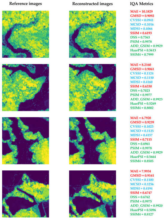
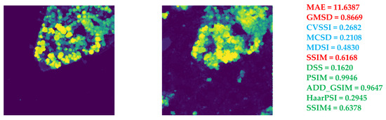
Figure 9.
Illustration of sample reconstructed CHM images (98th percentile) and high-resolution reference images for 576 m HHDCs together with the values of selected IQA metrics. The values of metrics that follow subjective perception are marked in green (higher is better) and blue (smaller is better); the others are marked in red.
Three of the recommended metrics, namely CVSSI, MSCD, and MDSI, marked in blue, have negative SROCC values, as presented in Table 2. Hence, their smaller values should be interpreted as reflecting higher quality, similarly to MAE. The four other metrics (ADD_GSIM, DSS, HaarPSI, MCSD, MDSI, PSIM, and SSIM4), marked in green, have positive SROCC values, similarly to SSIM; therefore, their higher values indicate better quality. One of the metrics with negative SROCC values, namely GMSD, demonstrated the smallest value for the lowest-quality image; hence, its final verification was negative, at least for assessing the reconstruction results of Canopy Height Models.
Thus, eight metrics, namely ADD_GSIM, DSS, HaarPSI, PSIM, SSIM4, CVSSI, MCSD, and MDSI, are recommended for further research, particularly related to the reconstruction of the CHMs.
6.4. Ablation Study on Hyperparameter Effects
To further validate the robustness of our generative diffusion model and assess the impact of key hyperparameters on reconstruction quality, we conducted an ablation study. This study systematically varies three critical hyperparameters—diffusion steps, illumination pattern type, and compression level—to evaluate their effects on the quality of reconstructed HHDCs and the presence of artifacts. The findings provide insights into optimizing our compressed sensing framework, with reconstruction quality measured using the IQA metrics outlined in Section 6.
6.4.1. Hyperparameters Tested
In our experiments, we investigated the effects of several key hyperparameters that significantly influence the model’s performance and computational efficiency. First, we examined the diffusion steps, which specify the number of reverse diffusion steps during the inference phase. This parameter directly impacts both the fidelity of the generated details and the computational resources required. To assess its influence, we tested settings of 50 steps, 100 steps, 250 steps, 500 steps, and 1000 steps (serving as the baseline). Next, we explored the sampling ratio, a crucial factor that determines the fraction of data retained in the low-resolution measurements, thereby affecting the compression level. We evaluated its impact using values of 6.25%, 12.5%, 25% (the baseline), and 50%. Finally, we assessed the illumination pattern type, which dictates how the scene is captured in the compressed measurements. For this hyperparameter, we experimented with three distinct patterns: random (the baseline), blue noise, and Bayer [77,78]. Both blue noise and Bayer patterns are engineered to minimize low-frequency components in the sampling process, which has been shown to enhance sampling efficiency and improve the quality of reconstructed signals [7]. By systematically varying these hyperparameters, we aimed to understand their individual and collective effects on the overall performance of our model.
6.4.2. Experimental Setup
The experiments utilized the algorithm and dataset described in Section 4.1 and Section 6.1, respectively. For diffusion steps, we adjusted the inference steps using the baseline model trained with 1000 steps. For compression level, we generated new measurements by varying the sampling ratio and illumination pattern. Reconstruction quality was assessed using the full-reference IQA metrics identified in Section 6: ADD_GSIM, DSS, HaarPSI, PSIM, SSIM4, CVSSI, MCSD, and MDSI. We also conducted qualitative evaluations by inspecting the reconstructed CHMs for artifacts like hallucinations or blurring.
6.4.3. Results
The ablation study results are presented in Table 3 and Figure 10 and Figure 11, showing the quantitative impact of each hyperparameter on reconstruction quality and artifact presence. Multiple examples are shown for both the CHM and DTM.
Table 3.
Ablation studies for multiple illumination patterns, sampling ratios, and diffusion sampling steps. We present SSIM for the CHM in all cases (higher is better, the best results are marked with bold fonts).
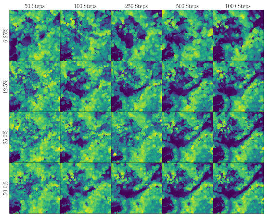
Figure 10.
Reconstructed CHMs for different settings: 6.25% sampling, 12.5% sampling, 25% sampling, 50% sampling, 50 diffusion steps, 100 diffusion steps, 250 diffusion steps, 500 diffusion steps, and 1000 diffusion steps. As we move from left to right, the number of diffusion steps increases. As we move from top to bottom, the sampling ratio increases. Smaller sampling ratios result in significant hallucinations.
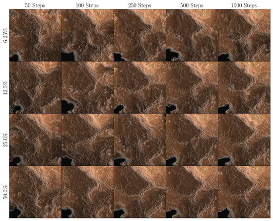
Figure 11.
Reconstructed DTMs for different settings: 6.25% sampling, 12.5% sampling, 25% sampling, 50% sampling, 50 diffusion steps, 100 diffusion steps, 250 diffusion steps, 500 diffusion steps, and 1000 diffusion steps. As we move from left to right, the number of diffusion steps increases. As we move from top to bottom, the sampling ratio increases. Smaller sampling ratios result in significant hallucinations.
6.4.4. Analysis and Discussion
Our findings suggest that higher sampling ratios significantly enhance reconstruction quality, with 50% sampling achieving near-ground-truth fidelity and minimal artifacts, while 6.25% sampling introduces noticeable hallucinations. Among the illumination patterns, blue noise slightly outperforms random and Bayer patterns at 25% sampling, likely due to its uniform coverage. Increasing the diffusion steps improves hallucinations: 50 steps result in heavy hallucinations in all the scenarios, while 1000 steps yield improved reconstructions, although at a higher computational cost. These results highlight the trade-offs between quality and efficiency, emphasizing the need to optimize compression levels and diffusion steps for practical satellite LiDAR applications.
7. Conclusions and Future Work
Spaceborne LiDAR systems are essential for detailed Earth observation, yet hardware limitations and data processing constraints pose significant challenges. This study introduces a novel framework combining compressed sensing and diffusion generative models, leveraging randomized illumination patterns to efficiently sample and compress LiDAR data onboard satellites. Ground-based diffusion models successfully reconstruct high-resolution Digital Terrain Models (DTMs) and Canopy Height Models (CHMs) from these sparse measurements, closely matching ground truth data. Rigorous evaluation using various image quality assessment (IQA) metrics—including ADD_GSIM, DSS, HaarPSI, PSIM, SSIM4, CVSSI, MCSD, and MDSI—demonstrated the robustness and practical utility of our method for ecological applications such as forest management and climate modeling. This work establishes a scalable, cost-effective approach that enhances LiDAR system performance without requiring extensive hardware upgrades. Future research will focus on further refining reconstruction algorithms to reduce artifacts and extending the methodology to additional sensing technologies, such as hyperspectral imaging. By streamlining data handling and ensuring accurate reconstruction, our approach promises significant advancements in environmental monitoring, supporting biodiversity conservation, disaster preparedness, and sustainable resource management.
Author Contributions
Conceptualization, A.R.-J., G.R.A., V.L. and K.O.; methodology, A.R.-J., N.P.-D., G.R.A., V.L. and K.O.; software, A.R.-J., N.P.-D., A.R., O.I., M.K. and P.L.; validation, G.R.A., V.L. and K.O.; formal analysis, A.R.-J., G.R.A. and V.L.; investigation, A.R.-J., G.R.A., V.L., M.K. and K.O.; resources, A.R.-J., N.P.-D., G.R.A., M.K., J.F. and P.L.; data curation, A.R.-J., N.P.-D., O.I. and M.K.; writing—original draft preparation, A.R.-J., N.P.-D., O.I., V.L. and K.O.; writing—review and editing, G.R.A., V.L. and K.O.; visualization, A.R.-J., J.F. and P.L.; supervision, G.R.A., V.L. and K.O.; project administration, G.R.A., V.L. and K.O.; funding acquisition, G.R.A., V.L. and K.O. All authors have read and agreed to the published version of the manuscript.
Funding
This research was funded in part by US National Science Foundation NSF under Grant No. 2404740, Science & Technology Center in Ukraine (STCU) Agreement No. 7116, and National Science Centre, Poland (NCN), Grant no. 2023/05/Y/ST6/00197, within the joint IMPRESS-U project entitled “EAGER IMPRESS-U: Exploratory Research on Generative Compression for Compressive Lidar”.
Institutional Review Board Statement
Not applicable.
Informed Consent Statement
Not applicable.
Data Availability Statement
The original data (emulated HHDCs) presented in the study are openly available at https://doi.org/10.34808/3dk4-ah25. The raw LiDAR data regarding the Smithsonian Environmental Research Center (SERC) in the state of Maryland are available at NEON (National Ecological Observatory Network) website: Discrete return LiDAR point cloud (DP1.30003.001), RELEASE-2024. https://doi.org/10.48443/hj77-kf64. Further inquiries can be directed to the authors.
Conflicts of Interest
The authors declare no conflicts of interest. The funders had no role in the design of the study; in the collection, analyses, or interpretation of data; in the writing of the manuscript; or in the decision to publish the results.
Abbreviations
The following abbreviations are used in this manuscript:
| ADD | Analysis of Distortion Distribution |
| CASALS | Concurrent Artificially Intelligent Spectrometry and Adaptive LiDAR System |
| CHM | Canopy Height Model |
| CHP | Canopy Height Profile |
| CORNIA | Codebook Representation for No-Reference Image Assessment |
| CSF | Contrast Sensitivity Function |
| CSRIQ | Compressive Sensing Recovered Image Quality |
| CSSIM | Color Structural Similarity |
| CVSSI | Contrast- and Visual-Saliency-Similarity-Induced Index |
| CW-SSIM | Complex Wavelet Structural Similarity |
| DCT | Discrete Cosine Transform |
| DDPM | Denoising Diffusion Probabilistic Model |
| DEM | Digital Elevation Model |
| DPS | Diffusion Posterior Sampling |
| DSI | Dissimilarity Index |
| DSM | Digital Surface Model |
| DSS | DCT Sub-Band Similarity |
| DTM | Digital Terrain Model |
| ESSIM | Edge Strength SIMilarity |
| FR IQA | Full-Reference Image Quality Assessment |
| FSIM | Feature Similarity |
| FWHM | Full Width at Half Maximum |
| GEDI | Global Ecosystem Dynamics Investigation |
| G-LiHT | Goddard’s LiDAR, Hyperspectral, and Thermal (Airborne Imager) |
| GMSD | Gradient Magnitude Similarity Deviation |
| GSIM | Gradient Similarity |
| GT | Ground Truth |
| HaarPSI | Haar Wavelet-Based Perceptual Similarity Index |
| HHDC | Hyperheight Data Cube |
| HVS | Human Visual System |
| ICESat | Ice, Cloud, and Land Elevation Satellite |
| IFC | Image Fidelity Criterion |
| IFS | Independent Feature Similarity |
| IGM | Internal Generative Mechanism |
| JND | Just-Noticeable Distortions |
| KL | Kullback–Leibler (Divergence) |
| LiDAR | Light Detection and Ranging |
| ML | Machine Learning |
| MAD | Most Apparent Distortion |
| MAE | Mean Absolute Error |
| MCSD | Multiscale Contrast Similarity Deviation |
| MDSI | Mean Deviation Similarity Index |
| MOS | Mean Opinion Score |
| MSE | Mean Squared Error |
| MS-SSIM | Multiscale Structural Similarity |
| NASA | National Aeronautics and Space Administration |
| NEON | National Ecological Observatory Network |
| NQM | Noise Quality Measure |
| NSF | National Science Foundation |
| PLCC | Pearson’s Linear Correlation Coefficient |
| PSIM | Perceptual Similarity |
| PSNR | Peak Signal-to-Noise Ratio |
| QILV | Quality Index based on Local Variance |
| RFSIM | Riesz Transform-based Feature Similarity |
| RVSIM | Riesz Transform and Visual-Contrast-Sensitivity-based Feature Similarity Index |
| SDE | Stochastic Differential Equation |
| SERC | Smithsonian Environmental Research Center |
| SFF | Sparse Feature Fidelity |
| SROCC | Spearman’s Rank-Order Correlation Coefficient |
| SR-SIM | Spectral-Residual-based Similarity |
| SSIM | Structural Similarity |
| SVD | Singular Value Decomposition |
| TID | Tampere Image Database |
| UIQI | Universal Image Quality Index |
| UNIQUE | Unsupervised Image Quality Estimation |
| VIF | Visual Information Fidelity |
| VP | Variance-Preserving |
| VQEG | Video Quality Experts Group |
| VSI | Visual-Saliency-Induced Index |
| VSNR | Visual Signal-to-Noise Ratio |
| WASH | Wavelet-based Sharp Features |
| WSNR | Weighted Signal-to-Noise Ratio |
References
- Harding, D. Pulsed laser altimeter ranging techniques and implications for terrain mapping. In Topographic Laser Ranging and Scanning, 2nd ed.; Taylor & Francis, CRC Press: Boca Raton, FL, USA, 2018; pp. 201–220. [Google Scholar] [CrossRef]
- Neuenschwander, A.L.; Magruder, L.A. The potential impact of vertical sampling uncertainty on ICESat-2/ATLAS terrain and canopy height retrievals for multiple ecosystems. Remote Sens. 2016, 8, 1039. [Google Scholar] [CrossRef]
- Klemas, V. Beach profiling and LIDAR bathymetry: An overview with case studies. J. Coast. Res. 2011, 27, 1019–1028. [Google Scholar] [CrossRef]
- Hancock, S.; Armston, J.; Hofton, M.; Sun, X.; Tang, H.; Duncanson, L.I.; Kellner, J.R.; Dubayah, R. The GEDI simulator: A large-footprint waveform lidar simulator for calibration and validation of spaceborne missions. Earth Space Sci. 2019, 6, 294–310. [Google Scholar] [CrossRef] [PubMed]
- Tang, H.; Armston, J.; Hancock, S.; Marselis, S.; Goetz, S.; Dubayah, R. Characterizing global forest canopy cover distribution using spaceborne lidar. Remote Sens. Environ. 2019, 231, 111262. [Google Scholar] [CrossRef]
- Cook, B.D.; Corp, L.A.; Nelson, R.F.; Middleton, E.M.; Morton, D.C.; McCorkel, J.T.; Masek, J.G.; Ranson, K.J.; Ly, V.; Montesano, P.M. NASA Goddard’s LiDAR, hyperspectral and thermal (G-LiHT) airborne imager. Remote Sens. 2013, 5, 4045–4066. [Google Scholar] [CrossRef]
- Ramirez-Jaime, A.; Pena-Pena, K.; Arce, G.R.; Harding, D.; Stephen, M.; MacKinnon, J. HyperHeight LiDAR Compressive Sampling and Machine Learning Reconstruction of Forested Landscapes. IEEE Trans. Geosci. Remote Sens. 2024, 62, 1–16. [Google Scholar] [CrossRef]
- Ramirez-Jaime, A.; Porras-Diaz, N.; Arce, G.R.; Harding, D.; Stephen, M.; MacKinnon, J. Super-Resolution of Satellite Lidars for Forest Studies Via Generative Adversarial Networks. In Proceedings of the IGARSS 2024—2024 IEEE International Geoscience and Remote Sensing Symposium, Athens, Greece, 7–12 July 2024; pp. 2271–2274. [Google Scholar] [CrossRef]
- Ramirez-Jaime, A.; Arce, G.; Stephen, M.; MacKinnon, J. Super-resolution of satellite lidars for forest studies using diffusion generative models. In Proceedings of the 2024 IEEE Conference on Computational Imaging Using Synthetic Apertures (CISA), Boulder, CO, USA, 20–23 May 2024; IEEE: Piscataway, NJ, USA, 2024; pp. 01–05. [Google Scholar] [CrossRef]
- Porras-Diaz, N.; Ramirez-Jaime, A.; Arce, G.; Vargas, R.; Harding, D.; Stephen, M.; MacKinnon, J. Multi-Modal Transformer for Compressive LiDARs Using Hyperspectral Imaging Side-Information. In Proceedings of the IGARSS 2024—2024 IEEE International Geoscience and Remote Sensing Symposium, Athens, Greece, 7–12 July 2024; IEEE: Piscataway, NJ, USA, 2024; pp. 2451–2454. [Google Scholar] [CrossRef]
- Porras-Diaz, N.; Ramirez-Jaime, A.; Arce, G.R.; Pena-Pena, K.; Harding, D.; Stephen, M.; MacKinnon, J.; Vargas, R. Transformer End-to-End Optimization of Compressive Lidars using Imaging Spectroscopy Side-Information. IEEE Trans. Geosci. Remote Sens. 2024, 62, 1–17. [Google Scholar] [CrossRef]
- Arce, G.R.; Ramirez-Jaime, A.; Porras-Diaz, N. High altitude computational lidar emulation and machine learning reconstruction for Earth sciences. In Proceedings of the Big Data VI: Learning, Analytics, and Applications, National Harbor, MA, USA, 21–25 April 2024; SPIE: Bellingham, WA, USA, 2024; Volume 13036, pp. 25–30. [Google Scholar] [CrossRef]
- Ramirez-Jaime, A.; Porras-Diaz, N.; Arce, G.R.; Stephen, M. Super-Resolved 3-D Satellite Lidar Imaging of Earth via Generative Diffusion Models. IEEE Trans. Geosci. Remote Sens. 2025, 63, 1–19. [Google Scholar] [CrossRef]
- Candès, E.J.; Wakin, M.B. An introduction to compressive sampling. IEEE Signal Process. Mag. 2008, 25, 21–30. [Google Scholar] [CrossRef]
- Donoho, D.L. Compressed sensing. IEEE Trans. Inf. Theory 2006, 52, 1289–1306. [Google Scholar] [CrossRef]
- Khanna, S.; Liu, P.; Zhou, L.; Meng, C.; Rombach, R.; Burke, M.; Lobell, D.; Ermon, S. Diffusionsat: A generative foundation model for satellite imagery. arXiv 2023, arXiv:2312.03606. [Google Scholar]
- Xiao, Y.; Yuan, Q.; Jiang, K.; He, J.; Jin, X.; Zhang, L. EDiffSR: An efficient diffusion probabilistic model for remote sensing image super-resolution. IEEE Trans. Geosci. Remote Sens. 2023, 62, 3341437. [Google Scholar] [CrossRef]
- Ho, J.; Jain, A.; Abbeel, P. Denoising diffusion probabilistic models. Adv. Neural Inf. Process. Syst. 2020, 33, 6840–6851. [Google Scholar] [CrossRef]
- Song, Y.; Sohl-Dickstein, J.; Kingma, D.P.; Kumar, A.; Ermon, S.; Poole, B. Score-based generative modeling through stochastic differential equations. arXiv 2020, arXiv:2011.13456. [Google Scholar] [CrossRef]
- Sohl-Dickstein, J.; Weiss, E.; Maheswaranathan, N.; Ganguli, S. Deep Unsupervised Learning using Nonequilibrium Thermodynamics. In JMLR Workshop and Conference Proceedings, Proceedings of the 32nd International Conference on Machine Learning, ICML, Lille, France, 6–11 July 2015; Bach, F.R., Blei, D.M., Eds.; PMLR: London, UK, 2015; Volume 37, pp. 2256–2265. [Google Scholar]
- Anderson, B.D. Reverse-time diffusion equation models. Stoch. Process. Appl. 1982, 12, 313–326. [Google Scholar] [CrossRef]
- Chung, H.; Kim, J.; Mccann, M.T.; Klasky, M.L.; Ye, J.C. Diffusion posterior sampling for general noisy inverse problems. arXiv 2022, arXiv:2209.14687. [Google Scholar] [CrossRef]
- Robbins, H.E. An empirical Bayes approach to statistics. In Breakthroughs in Statistics: Foundations and Basic Theory; Kotz, S., Johnson, N., Eds.; Springer Series in Statistics; Springer: New York, NY, USA, 1992; pp. 388–394. [Google Scholar] [CrossRef]
- Wang, Z.; Li, Q. Information content weighting for perceptual image quality assessment. IEEE Trans. Image Process. 2011, 20, 1185–1198. [Google Scholar] [CrossRef]
- Palubinskas, G. Mystery behind similarity measures MSE and SSIM. In Proceedings of the 2014 IEEE International Conference on Image Processing (ICIP), Paris, France, 27–30 October 2014; IEEE: Piscataway, NJ, USA, 2014; pp. 575–579. [Google Scholar] [CrossRef]
- Zhai, G.; Min, X. Perceptual image quality assessment: A survey. Sci. China Inf. Sci. 2020, 63, 211301. [Google Scholar] [CrossRef]
- Salahdine, F.; Ghribi, E.; Kaabouch, N. Metrics for Evaluating the Efficiency of Compressing Sensing Techniques. In Proceedings of the 2020 International Conference on Information Networking (ICOIN), Barcelona, Spain, 7–10 January 2020; IEEE: Piscataway, NJ, USA, 2020; pp. 562–567. [Google Scholar] [CrossRef]
- Hu, B.; Li, L.; Wu, J.; Wang, S.; Tang, L.; Qian, J. No-reference quality assessment of compressive sensing image recovery. Signal Process. Image Commun. 2017, 58, 165–174. [Google Scholar] [CrossRef]
- Hu, B.; Li, L.; Wu, J.; Qian, J. Subjective and objective quality assessment for image restoration: A critical survey. Signal Process. Image Commun. 2020, 85, 115839. [Google Scholar] [CrossRef]
- Ye, P.; Kumar, J.; Kang, L.; Doermann, D. Unsupervised feature learning framework for no-reference image quality assessment. In Proceedings of the 2012 IEEE Conference on Computer Vision and Pattern Recognition (CVPR), Providence, RI, USA, 16–21 June 2012; IEEE: Piscataway, NJ, USA, 2012; pp. 1098–1105. [Google Scholar] [CrossRef]
- Qureshi, M.A.; Deriche, M.; Beghdadi, A.; Amin, A. A critical survey of state-of-the-art image inpainting quality assessment metrics. J. Vis. Commun. Image Represent. 2017, 49, 177–191. [Google Scholar] [CrossRef]
- Ponomarenko, N.; Jin, L.; Ieremeiev, O.; Lukin, V.; Egiazarian, K.; Astola, J.; Vozel, B.; Chehdi, K.; Carli, M.; Battisti, F.; et al. Image database TID2013: Peculiarities, results and perspectives. Signal Process. Image Commun. 2015, 30, 57–77. [Google Scholar] [CrossRef]
- Bondžulić, B.; Stojanović, N.; Lukin, V.; Kryvenko, S. JPEG and BPG visually lossless image compression via KonJND-1k database. Vojnoteh. Glas. 2024, 72, 1214–1241. [Google Scholar] [CrossRef]
- Streijl, R.C.; Winkler, S.; Hands, D.S. Mean opinion score (MOS) revisited: Methods and applications, limitations and alternatives. Multimed. Syst. 2014, 22, 213–227. [Google Scholar] [CrossRef]
- Gu, K.; Li, L.; Lu, H.; Min, X.; Lin, W. A fast reliable image quality predictor by fusing micro- and macro-structures. IEEE Trans. Ind. Electron. 2017, 64, 3903–3912. [Google Scholar] [CrossRef]
- Ponomarenko, N.; Ieremeiev, O.; Lukin, V.; Egiazarian, K.; Carli, M. Modified image visual quality metrics for contrast change and mean shift accounting. In Proceedings of the 2011 11th International Conference The Experience of Designing and Application of CAD Systems in Microelectronics (CADSM), Polyana-Svalyava, Ukraine, 23–25 February 2011; pp. 305–311. [Google Scholar]
- Xue, W.; Zhang, L.; Mou, X.; Bovik, A.C. Gradient Magnitude Similarity Deviation: A Highly Efficient Perceptual Image Quality Index. IEEE Trans. Image Process. 2014, 23, 684–695. [Google Scholar] [CrossRef]
- Wang, T.; Zhang, L.; Jia, H.; Li, B.; Shu, H. Multiscale contrast similarity deviation: An effective and efficient index for perceptual image quality assessment. Signal Process. Image Commun. 2016, 45, 1–9. [Google Scholar] [CrossRef]
- Wu, J.; Lin, W.; Shi, G.; Liu, A. Perceptual quality metric with internal generative mechanism. IEEE Trans. Image Process. 2013, 22, 43–54. [Google Scholar] [CrossRef]
- Ponomarenko, N.; Silvestri, F.; Egiazarian, K.; Carli, M.; Astola, J.; Lukin, V. On between-coefficient contrast masking of DCT basis functions. In Proceedings of the Third International Workshop on Video Processing and Quality Metrics for Consumer Electronics, VPQM 2007, Scottsdale, AZ, USA, 25–26 January 2007; Volume 4. [Google Scholar]
- Ponomarenko, M.; Egiazarian, K.; Lukin, V.; Abramova, V. Structural Similarity index with predictability of image blocks. In Proceedings of the 17th International Conference on Mathematical Methods in Electromagnetic Theory (MMET), Kiev, Ukraine, 2–5 July 2018; pp. 115–118. [Google Scholar] [CrossRef]
- Liu, A.; Lin, W.; Narwaria, M. Image Quality Assessment Based on Gradient Similarity. IEEE Trans. Image Process. 2012, 21, 1500–1512. [Google Scholar] [CrossRef]
- Egiazarian, K.; Astola, J.; Ponomarenko, N.; Lukin, V.; Battisti, F.; Carli, M. Two new full-reference quality metrics based on HVS. In Proceedings of the Second International Workshop on Video Processing and Quality Metrics, Scottsdale, AZ, USA, 22–24 January 2006; Volume 4. [Google Scholar]
- Reisenhofer, R.; Bosse, S.; Kutyniok, G.; Wiegand, T. A Haar wavelet-based perceptual similarity index for image quality assessment. Signal Process. Image Commun. 2018, 61, 33–43. [Google Scholar] [CrossRef]
- Zhang, X.; Feng, X.; Wang, W.; Xue, W. Edge Strength Similarity for Image Quality Assessment. IEEE Signal Process. Lett. 2013, 20, 319–322. [Google Scholar] [CrossRef]
- Nafchi, H.Z.; Shahkolaei, A.; Hedjam, R.; Cheriet, M. Mean Deviation Similarity Index: Efficient and reliable full-reference image quality evaluator. IEEE Access 2016, 4, 5579–5590. [Google Scholar] [CrossRef]
- Jia, H.; Zhang, L.; Wang, T. Contrast and Visual Saliency Similarity-Induced index for assessing image quality. IEEE Access 2018, 6, 65885–65893. [Google Scholar] [CrossRef]
- Zhang, L.; Shen, Y.; Li, H. VSI: A Visual Saliency-Induced Index for Perceptual Image Quality Assessment. IEEE Trans. Image Process. 2014, 23, 4270–4281. [Google Scholar] [CrossRef]
- Gu, K.; Wang, S.; Zhai, G.; Lin, W.; Yang, X.; Zhang, W. Analysis of Distortion Distribution for Pooling in Image Quality Prediction. IEEE Trans. Broadcast. 2016, 62, 446–456. [Google Scholar] [CrossRef]
- Zhang, L.; Li, H. SR-SIM: A fast and high performance IQA index based on spectral residual. In Proceedings of the 2012 19th IEEE International Conference on Image Processing, Orlando, FL, USA, 30 September–3 October 2012; pp. 1473–1476. [Google Scholar] [CrossRef]
- Balanov, A.; Schwartz, A.; Moshe, Y.; Peleg, N. Image quality assessment based on DCT subband similarity. In Proceedings of the International Conference on Image Processing (ICIP), Quebec City, QC, Canada, 27–30 September 2015; pp. 2105–2109. [Google Scholar] [CrossRef]
- Dumic, E.; Grgic, S.; Grgic, M. IQM2: New image quality measure based on steerable pyramid wavelet transform and structural similarity index. SIViP 2014, 8, 1159–1168. [Google Scholar] [CrossRef]
- Zhang, L.; Zhang, L.; Mou, X.; Zhang, D. FSIM: A feature similarity index for image quality assessment. IEEE Trans. Image Process. 2011, 20, 2378–2386. [Google Scholar] [CrossRef]
- Chandler, D.M. Most apparent distortion: Full-reference image quality assessment and the role of strategy. J. Electron. Imaging 2010, 19, 011006. [Google Scholar] [CrossRef]
- Chang, H.W.; Zhang, Q.W.; Wu, Q.G.; Gan, Y. Perceptual image quality assessment by independent feature detector. Neurocomputing 2015, 151, 1142–1152. [Google Scholar] [CrossRef]
- Temel, D.; Prabhushankar, M.; AlRegib, G. UNIQUE: Unsupervised Image Quality Estimation. IEEE Signal Process. Lett. 2016, 23, 1414–1418. [Google Scholar] [CrossRef]
- Chang, H.W.; Yang, H.; Gan, Y.; Wang, M.H. Sparse Feature Fidelity for perceptual image quality assessment. IEEE Trans. Image Process. 2013, 22, 4007–4018. [Google Scholar] [CrossRef] [PubMed]
- Li, S.; Zhang, F.; Ma, L.; Ngan, K.N. Image Quality Assessment by Separately Evaluating Detail Losses and Additive Impairments. IEEE Trans. Multimed. 2011, 13, 935–949. [Google Scholar] [CrossRef]
- Wang, Z.; Simoncelli, E.P.; Bovik, A.C. Multiscale structural similarity for image quality assessment. In Proceedings of the 37th Asilomar Conference on Signals, Systems and Computers, Pacific Grove, CA, USA, 9–12 November 2003; pp. 1398–1402. [Google Scholar] [CrossRef]
- Mitsa, T.; Varkur, K. Evaluation of contrast sensitivity functions for the formulation of quality measures incorporated in halftoning algorithms. In Proceedings of the IEEE International Conference on Acoustics Speech and Signal Processing, Minneapolis, MN, USA, 27–30 April 1993; Volume 5, pp. 301–304. [Google Scholar] [CrossRef]
- Wang, Z.; Bovik, A.C.; Sheikh, H.R.; Simoncelli, E.P. Image quality assessment: From error visibility to structural similarity. IEEE Trans. Image Process. 2004, 13, 600–612. [Google Scholar] [CrossRef] [PubMed]
- Damera-Venkata, N.; Kite, T.; Geisler, W.S.; Evans, B.L.; Bovik, A.C. Image quality assessment based on a degradation model. IEEE Trans. Image Process. 2000, 9, 636–650. [Google Scholar] [CrossRef]
- Yang, G.; Li, D.; Lu, F.; Liao, Y.; Yang, W. RVSIM: A feature similarity method for full-reference image quality assessment. J. Image Video Proc. 2018, 2018, 6. [Google Scholar] [CrossRef]
- Zhou, F.; Lu, Z.; Wang, C.; Sun, W.; Xia, S.T.; Liao, Q. Image Quality Assessment Based on Inter-Patch and Intra-Patch Similarity. PLoS ONE 2015, 10, e0116312. [Google Scholar] [CrossRef]
- Sheikh, H.R.; Bovik, A.C. Image information and visual quality. IEEE Trans. Image Process. 2006, 15, 430–444. [Google Scholar] [CrossRef]
- Chandler, D.; Hemami, S. VSNR: A Wavelet-Based Visual Signal-to-Noise Ratio for Natural Images. IEEE Trans. Image Process. 2007, 16, 2284–2298. [Google Scholar] [CrossRef]
- Zhang, L.; Zhang, L.; Mou, X. RFSIM: A feature based image quality assessment metric using Riesz transforms. In Proceedings of the 2010 IEEE International Conference on Image Processing, Hong Kong, 26–29 September 2010; pp. 321–324. [Google Scholar] [CrossRef]
- Aja-Fernandez, S.; Estepar, R.S.J.; Alberola-Lopez, C.; Westin, C.F. Image Quality Assessment based on Local Variance. In Proceedings of the 2006 International Conference of the IEEE Engineering in Medicine and Biology Society, New York, NY, USA, 30 August–3 September 2006; pp. 4815–4818. [Google Scholar] [CrossRef]
- Egiazarian, K.; Ponomarenko, M.; Lukin, V.; Ieremeiev, O. Statistical Evaluation of Visual Quality Metrics for Image Denoising. In Proceedings of the 2018 IEEE International Conference on Acoustics, Speech and Signal Processing (ICASSP), Calgary, AB, Canada, 15–20 April 2018; pp. 6752–6756. [Google Scholar] [CrossRef]
- Sheikh, H.R.; Bovik, A.C.; de Veciana, G. An information fidelity criterion for image quality assessment using natural scene statistics. IEEE Trans. Image Process. 2005, 14, 2117–2128. [Google Scholar] [CrossRef]
- Wang, Z.; Bovik, A.C. A universal image quality index. IEEE Signal Process. Lett. 2002, 9, 81–84. [Google Scholar] [CrossRef]
- Sampat, M.P.; Wang, Z.; Gupta, S.; Bovik, A.C.; Markey, M.K. Complex Wavelet Structural Similarity: A New Image Similarity Index. IEEE Trans. Image Process. 2009, 18, 2385–2401. [Google Scholar] [CrossRef] [PubMed]
- Reenu, M.; David, D.; Raj, S.S.A.; Nair, M.S. Wavelet Based Sharp Features (WASH): An Image Quality Assessment Metric Based on HVS. In Proceedings of the 2013 2nd International Conference on Advanced Computing, Networking and Security, Mangalore, India, 15–17 December 2013; pp. 79–83. [Google Scholar] [CrossRef]
- Shnayderman, A.; Gusev, A.; Eskicioglu, A. An SVD-based grayscale image quality measure for local and global assessment. IEEE Trans. Image Process. 2006, 15, 422–429. [Google Scholar] [CrossRef] [PubMed]
- Loescher, H.W.; Kelly, E.F.; Lea, R. National ecological observatory network: Beginnings, programmatic and scientific challenges, and ecological forecasting. In Terrestrial Ecosystem Research Infrastructures; CRC Press: Boca Raton, FL, USA, 2017; pp. 27–52. [Google Scholar] [CrossRef]
- National Ecological Observatory Network (NEON). Discrete Return LiDAR Point Cloud (DP1.30003.001); National Ecological Observatory Network (NEON): New York, NY, USA, 2024. [Google Scholar] [CrossRef]
- Lau, D.L.; Arce, G.R.; Gallagher, N.C. Digital halftoning by means of green-noise masks. J. Opt. Soc. Am. A 1999, 16, 1575–1586. [Google Scholar] [CrossRef]
- Lau, D.L.; Ulichney, R.; Arce, G.R. Blue and green noise halftoning models. IEEE Signal Process. Mag. 2003, 20, 28–38. [Google Scholar] [CrossRef]
Disclaimer/Publisher’s Note: The statements, opinions and data contained in all publications are solely those of the individual author(s) and contributor(s) and not of MDPI and/or the editor(s). MDPI and/or the editor(s) disclaim responsibility for any injury to people or property resulting from any ideas, methods, instructions or products referred to in the content. |
© 2025 by the authors. Licensee MDPI, Basel, Switzerland. This article is an open access article distributed under the terms and conditions of the Creative Commons Attribution (CC BY) license (https://creativecommons.org/licenses/by/4.0/).