Article

Map of Arctic and Antarctic Polynyas 2013–2022 Using Sea Ice Concentration

1
National Key Laboratory of Earth System Numerical Modeling and Application, College of Earth and Planetary Sciences, University of Chinese Academy of Sciences, Beijing 100049, China
2
State Key Laboratory of Resources and Environmental Information System, Institute of Geographic Sciences and Natural Resources Research, Chinese Academy of Sciences, Beijing 100101, China
3
School of Mathematics and Maxwell Institute for Mathematical Sciences, The University of Edinburgh, Edinburgh EH1 2LE, UK
*
Author to whom correspondence should be addressed.
Remote Sens. 2025, 17(7), 1213; https://doi.org/10.3390/rs17071213
Submission received: 24 February 2025 / Revised: 26 March 2025 / Accepted: 27 March 2025 / Published: 28 March 2025
(This article belongs to the Special Issue SAR Monitoring of Marine and Coastal Environments)

Abstract

:
Polynyas play a crucial role in polar ecosystems, influencing biodiversity, climate regulation, and oceanic processes. This study employs Synthetic Aperture Radar (SAR) data to determine the optimal sea ice concentration threshold for polynya identification, which is established at 75%. We present a dataset of daily polynya distribution in the Arctic and Antarctic from 2013 to 2022, analyzing their spatial patterns, interannual variability, and seasonal dynamics. Our results indicate that coastal polynyas, primarily located near landmasses, dominate both polar regions. The total polynya area in the Antarctic remained relatively stable, averaging approximately 1.86 × 10⁸ km2 per year, with an interannual fluctuation of −3.1 × 10⁵ km2 per year. In the Arctic, the average polynya area is around 1.59 × 10⁸ km2 per year, with an interannual fluctuation of −7.1 × 10⁵ km2 per year. Both regions exhibit distinct seasonal cycles: Arctic polynyas peak in May and reach their minimum in September, whereas Antarctic polynyas expand in November and contract to their smallest extent in February. The polynya formation and development result from a complex interplay of multiple factors, with no single variable fully explaining variations in polynyas’ extent. Additionally, the polynya area in the NOW, and Weddell Sea polynyas, exhibit consistent trends with chlorophyll-a concentration, highlighting their role as critical habitats for primary productivity in polar regions. These findings provide key insights into polynya dynamics and their broader implications for climate and ecological processes in polar regions.

1. Introduction

Polynyas, which are areas of open water or thin ice surrounded by thicker sea ice, play a crucial role in global ocean circulation, climate change, and polar ecosystems [1,2,3]. Polynyas are broadly categorized into two types: coastal polynyas and open-ocean polynyas. Coastal polynyas are typically driven by strong katabatic winds or ocean currents, which disperse sea ice and left open water areas [4,5,6]. Open-ocean polynyas are often associated with oceanic circulation and deep convection [7]. Polynya distribution exhibits strong regional characteristics, with Antarctic polynyas concentrated in the Weddell Sea, Ross Sea, and off the Adélie Coast, while Arctic polynyas mainly occurred in the Barents Sea, Greenland Sea, Okhotsk Sea, Kara and Laptev seas [3,6,8,9].
Polynyas significantly influence polar ecosystems and global climate [10,11,12]. Firstly, Polynyas, often referred to as “sea ice factories”, undergo freezing and salt rejection processes, generating substantial amounts of new ice [13]. For example, coastal polynyas occupy merely 1% of the Antarctic sea ice area, contributing up to 10% of Antarctica’s total sea ice production [12]. The salt expelled during this ice formation process is vital in the formation of Antarctic Bottom Water [14,15]. Likewise the Kara and Laptev Seas are often referred to as the Arctic’s “ice factories” due to their critical role in sea ice production [16]. Secondly, polynyas serve as hotspots for primary productivity, as open water allows greater penetration of solar radiation, promoting phytoplankton blooms and supporting higher trophic levels [17,18]. And, polynyas act as important carbon sinks, facilitating the transfer of atmospheric CO₂ to the deep ocean via the biological pump [11].
Current researches on polar polynyas rely on satellite remote sensing, in situ observations, and numerical modeling or their combinations [19,20,21]. Satellite remote sensing provides wide-area coverage and frequent observations, making it ideal for monitoring changes in polynya dynamics [22]. For instance, passive microwave and thermal infrared satellite data have been utilized to assess polynya characteristics and ice production in regions of the Laptev Sea and the North Water (NOW) Polynya [23,24]. In situ observations provide detailed, localized data on physical and biological processes within polynyas [25,26]. These observations are crucial for validating satellite data and improving the accuracy of numerical models. Numerical modelling simulates the complex interactions between the atmosphere, ocean, and sea ice, offering insights into the mechanisms driving polynya formation and evolution [27]. Models have been employed to evaluate sea ice concentration (SIC) and dynamical processes in various regions, such as the Laptev Sea, by integrating atmospheric forcing data and sea-ice/ocean models [16,28].
Recent advances in satellite systems have enabled the development of a diverse array of sea ice products derived from multiple sensors [29,30,31]. For example, brightness temperature measurements from spaceborne microwave radiometers are used to retrieve SIC [32,33,34], whereas sea ice thickness is estimated using data acquired by the Altimeter satellite [35] and Soil Moisture and Ocean Salinity satellite [36,37]. Additionally, Global Navigation Satellite System-Reflectometry data have been successfully employed to derive both sea ice concentration and thickness [38,39]. These enhancements in spatial and temporal resolution in the Arctic and Antarctic regions have significantly facilitated large-scale, long-term studies, particularly those focusing on polynyas [12,40].
Winsor and Bjtrk [41] analyzed reanalysis datasets of wind and temperature to assess sea ice production in the Arctic from 1958 to 1997, uncovering significant interannual variability in polynya ice production. Tamura and Ohshima [42] estimated sea ice production in Arctic coastal polynyas from 1992 to 2007 using microwave radiometer and imaging instruments, identifying a strong interannual correlation between sea ice production and polynya area. Dai et al. [43] calculated sea ice production in the Ross Ice Shelf Polynya (RISP) during 2017–2018 utilizing Sentinel-1 Synthetic Aperture Radar (SAR) data. Nakata et al. [6], employing the AMSR-E thin ice algorithm [44], generated daily data for the Southern Ocean from 2003 to 2010, focusing on ice types, thin ice thickness, and sea ice production during the winter months (March–October). Lin et al. [9] provided daily delineations of each Antarctic polynya from 2003 to 2022 based on SIC. Arrigo et al. [45] examined the relative importance of six environmental factors in controlling phytoplankton biomass and net primary production rates in 46 coastal polynyas around Antarctica, finding that chlorophyll-a concentration variations are closely linked to polynya area and ice shelf basal melting. These studies predominantly utilize satellite data and sea ice products to analyze sea ice production, polynya area changes, and their associations with environmental factors in the Arctic, Antarctic, or specific polynyas. However, a comprehensive global-scale analysis of polynya changes remains absent.
Currently, daily-resolution sea ice products, such as SIC, have been extensively applied to the delineation and study of polynyas covering both poles [9,19,46,47,48]. However, the SIC thresholds used vary considerably among studies [9,19,49,50]. Kern et al. [19] identified thin ice regions using thresholds ranging from 65% to 80%, while Smedsrud et al. [49] defined polynya boundaries within a 60–70% concentration range. Similarly, Massom et al. [50] adopted a 75% threshold, whereas Lin et al. [9] applied a 60% criterion for extracting Antarctic polynyas. These discrepancies suggest that the optimal SIC threshold for accurately determining polynya area and distribution remains ambiguous.
In this study, we conduct a pan-polar analysis of polynya dynamics across three integrated dimensions: spatiotemporal patterns, interannual-to-seasonal variability, and chlorophyll-a response mechanisms. Leveraging multi-sensor satellite observations from 2013 to 2022, we address three key aspects: (1) determining the optimal SIC threshold for extracting polynyas by correlating SAR data with SIC; (2) analyzing decadal changes and seasonal variations in polynya area in both the Arctic and Antarctic; and (3) investigating the relationships among polynya area, chlorophyll-a concentrations, and other environmental parameters (e.g., sea surface temperature, wind speed, total cloud cover). We aim to elucidate the dynamic behavior of polynyas and their coupling with primary production, thereby providing valuable insights for future polar ecosystem research.
The paper is structured as follows. Section 2 introduces the datasets, including Sentinel-1 SAR, SIC, chlorophyll-a concentration, and the other environmental parameters. Section 3 describes the methodology, which primarily consists of two parts: determining the optimal SIC threshold for polynya extraction and developing a systematic approach to identify polar polynyas in both hemispheres using specific SIC thresholds. Section 4 presents the results and discussion, focusing on the spatial distribution characteristics of Arctic and Antarctic polynyas, along with their interannual and seasonal variability patterns and discusses the potential relationship among polynya area, chlorophyll-a concentration and other environmental parameters. Finally, the conclusion and discussion are presented in Section 5.

2. Dataset

Three primary datasets are employed in this study: SIC data from the University of Bremen, Sentinel-1 SAR imagery provided by the European Space Agency (ESA), and datasets comprising chlorophyll-a and various environmental parameters. The Sentinel-1 SAR dataset is used to determine the optimal SIC threshold for polynya extraction. The SIC data enabled the identification of polynyas in both the Antarctic and Arctic regions, while the chlorophyll-a and environmental parameters facilitated an analysis of the relationships among polynya area, chlorophyll-a, and other key variables.

2.1. Sea Ice Concentration

The SIC utilized in this study are obtained from the University of Bremen’s Institute of Environmental Physics (https://data.seaice.uni-bremen.de/, accessed on 20 January 2025), derived from passive microwave sensors onboard satellites, including SSM/I, SSMIS, AMSR-E, and AMSR2. The data are processed using the ASI (ARTIST Sea Ice) algorithm [44], which leverages 89 GHz frequency channels to estimate SIC with spatial resolution of 6.25 km. The dataset provides daily coverage of the polar regions, encompassing the Arctic (north of 50°N) and Antarctic (south of 50°S).

2.2. Sentinel-1 SAR Images

The SAR images utilized in this study are from the ESA (https://dataspace.copernicus.eu, accessed on 20 January 2025) Sentinel-1 mission with C-band SAR observation, specifically the Extra Wide Swath (EW GRDM) mode. The EW mode offers a pixel spacing of approximately 40 m. The swath width is 400 km. The high spatial resolution and with swath make it particularly suitable for monitoring polynyas.

2.3. The Chlorophyll-a Concentration and the Environmental Parameters

Chlorophyll-a concentration in this study is derived from the Level-3 ocean color products provided by the European Space Agency (www.oceancolour.org, accessed on 20 January 2025). This dataset integrates observations from multiple sensors, including Orbview-2, Aqua, Envisat, Suomi-NPP, Sentinel-3A, and Sentinel-3B, and offers daily gridded products at a spatial resolution of 4 km [51]. Environmental parameters are obtained from ERA5 (https://cds.climate.copernicus.eu/, accessed on 20 January 2025) including variables such as 10 m wind speed (WS), sea surface temperature (SST), clear-sky direct solar radiation at the surface (Cdir), and total cloud cover (Tcc). These parameters are closely associated with the variations of polynyas area and phytoplankton biomass, exhibiting distinct seasonal and regional correlation patterns [52]. Wind speed influences the vertical transport of nutrients and phytoplankton by affecting the formation of polynyas and the intensity of vertical mixing, while the impact of cloud cover on the ecosystems is determined by the balance between visible light and ultraviolet radiation [53]. Moreover, sea surface temperature is strongly correlated with marine biomass and the occurrence of polynyas [3]. Consequently, we conducted a correlation analysis among polynyas area, chlorophyll-a content, and other environmental parameters in representative polynyas regions, aiming to elucidate the relationships among these variables in the development of polynyas.

3. Methods

3.1. Determining the Threshold for Extracting Polynyas from SIC

The spatial extent of polynyas exhibits notable seasonal variations. During winter, polynya areas generally remain stable, ranging between 10 and 105 km2 [54]. In contrast, summer conditions characterized by sea ice melt and the expansion of open water can lead to a substantial increase in polynya size, with maximum areas exceeding 1 × 10⁵ km2 [45] and, in some cases (e.g., the Ross Sea Polynya in 2014 [55]), reaching up to 836,590 km2. Given the relatively coarse spatial resolution of SIC data at 6.25 km, establishing an optimal SIC threshold is essential for accurately delineating the spatial distribution and extent of polynyas. While previous studies have employed SIC thresholds of 60%, 70%, and 75%, a consensus on the optimal threshold has yet to be reached [9,19,50].
In this study, we determined the optimal sea ice concentration (SIC) threshold for identifying polynyas by analyzing 20 SAR imageries from both the Arctic and Antarctic, covering typical coastal and open-ocean polynyas. Figure 1 illustrates three representative examples of classic polynyas from Arctic and Antarctic. Figure 1a1 depicts a typical Arctic coastal polynya located north of Wrangel Island, characterized by wind-induced features with a rough surface and distinct wind-driven ripples. The corresponding SAR image was acquired on 4 April 2020. Figure 1b1 illustrates an open-ocean Arctic polynya situated northwest of Severnaya Zemlya (Vize Island), featuring a relatively calm surface with faint wind-driven ripples and exhibiting a backscatter intensity significantly lower than adjacent sea ice regions. The associated Sentinel-1 SAR data were recorded on 2 February 2020. Finally, Figure 1c1 depicts the Weddell Sea Polynya, a quintessential Antarctic coastal polynya primarily driven by katabatic wind forcing. The Sentinel-1 image was acquired on 4 May 2020, during austral autumn sea ice expansion phase.
To determine the optimal SIC threshold, we adopted the following steps:
(1)
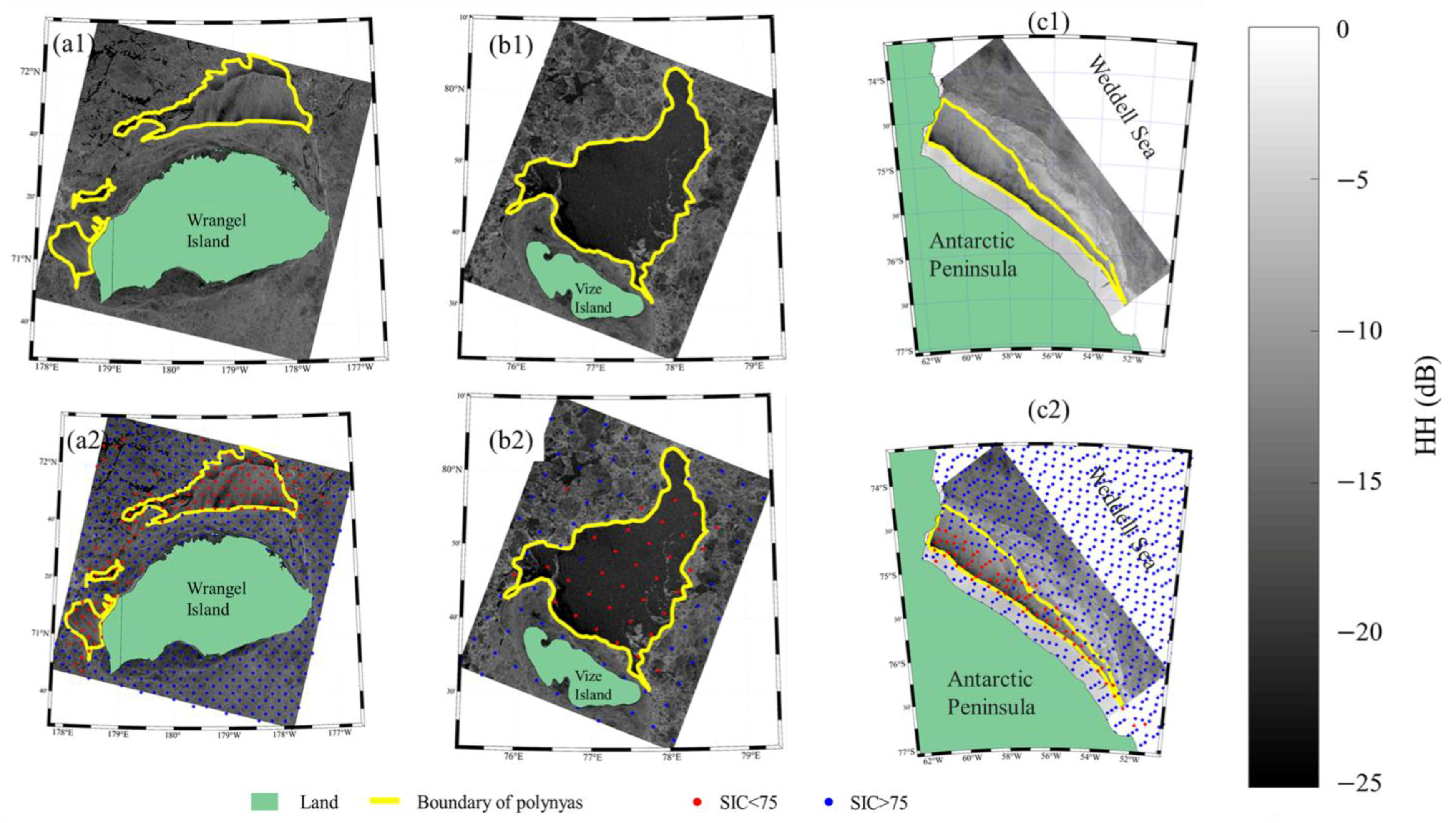
SAR-Based Delineation: we manually delineated polynya boundaries from high-resolution SAR images to capture detailed ice edge features and polynya morphology.
(2)
SIC-Based Extraction: polynyas are extracted from SIC data using thresholds ranging from 50% to 80% in 5% increments.
(3)
Comparison and Optimization: we compared the polynya areas derived from SIC with those obtained from SAR-based delineation. The SIC threshold that minimized the discrepancy between the two datasets is selected as optimal.
This approach ensured that the chosen SIC threshold accurately reflected the spatial extent of polynyas while minimizing errors inherent in SIC-based extraction.
Figure 2 illustrates that as the SIC threshold for polynya extraction increases, the delineated polynya area gradually increases (the red lines keep increasing). The green bars indicate the differences between the areas derived from SIC data and those delineated from SAR images. Notably, the absolute difference initially decreases with increasing thresholds then rises. Figure 2 also reveals that larger polynya areas are associated with greater extraction errors when using SIC data. However, across different polynya types, a threshold of 75% consistently minimizes this error.
Based on expert visual interpretation, the polynya boundaries have been delineated using yellow lines as shown in Figure 1a2–c2. The figures show the distribution of SIC greater than the threshold 75%, denoted by blue points, while SIC less than 75% is represented by red points. The red points are predominantly located within the delineated polynya areas, while points with SIC greater than 75% (blue points) are mostly located outside the delineated polynya areas. This suggests that using a 75% SIC threshold for polynya extraction not only ensures consistency in polynya area but also maintains accuracy in determining polynya locations. In an additional 17 SAR images analyzed for polynya delineation (see Supplementary Materials for details), the SIC-based extraction results are consistent with those obtained from the three representative SAR images discussed above. Consequently, a 75% SIC threshold is adopted for polynya extraction in this study.

3.2. Extracting Polar Polynyas from SIC

This section details the methodology employed to extract polynyas in polar regions using SIC data. The key steps are outlined as follows:
(1)
Binarization with SIC:
Figure 3a1,a2 displays the Arctic and Antarctic SIC distribution. Figure 3b1,b2 is the binarized image using a SIC threshold of 75%. Pixels with SIC values greater than or equal to 75% are classified as sea ice (denoted by red color), while pixels with SIC values less than 75% are classified as open water or potential polynya areas (denoted by blue color).
(2)
Identification of Isolated Open Water Regions:
The binarized image is analyzed to identify isolated regions of open water (pixels with a value of 1) are shown in Figure 3c1,c2. This is achieved by detecting eight-connected domains—regions where pixels are connected horizontally, vertically, or diagonally [56].
(3)
Filtering Out Large Connected Regions and outside of Marginal Ice Zone (MIZ):
To exclude large open-water areas that do not qualify as polynyas, connected regions exceeding 10⁶ km2 are removed. This ensures that only smaller, isolated regions are retained for further analysis. Simultaneously, MIZ is defined using a SIC threshold of 15% to 80% [57], delineating the boundaries of Arctic sea ice. Isolated units within the defined MIZ are excluded. The final extracted polynya areas are shown in Figure 3d1,d2, where blue regions represent polynyas identified based on SIC.

4. Results and Discussion

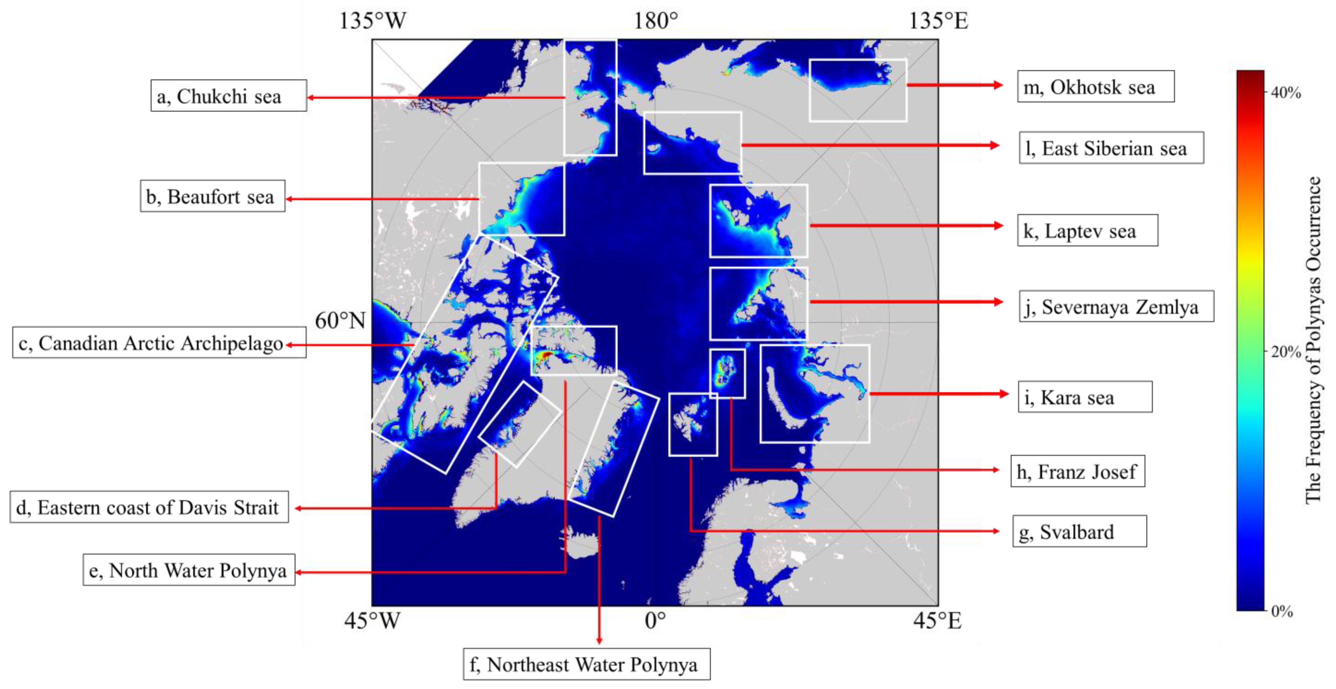
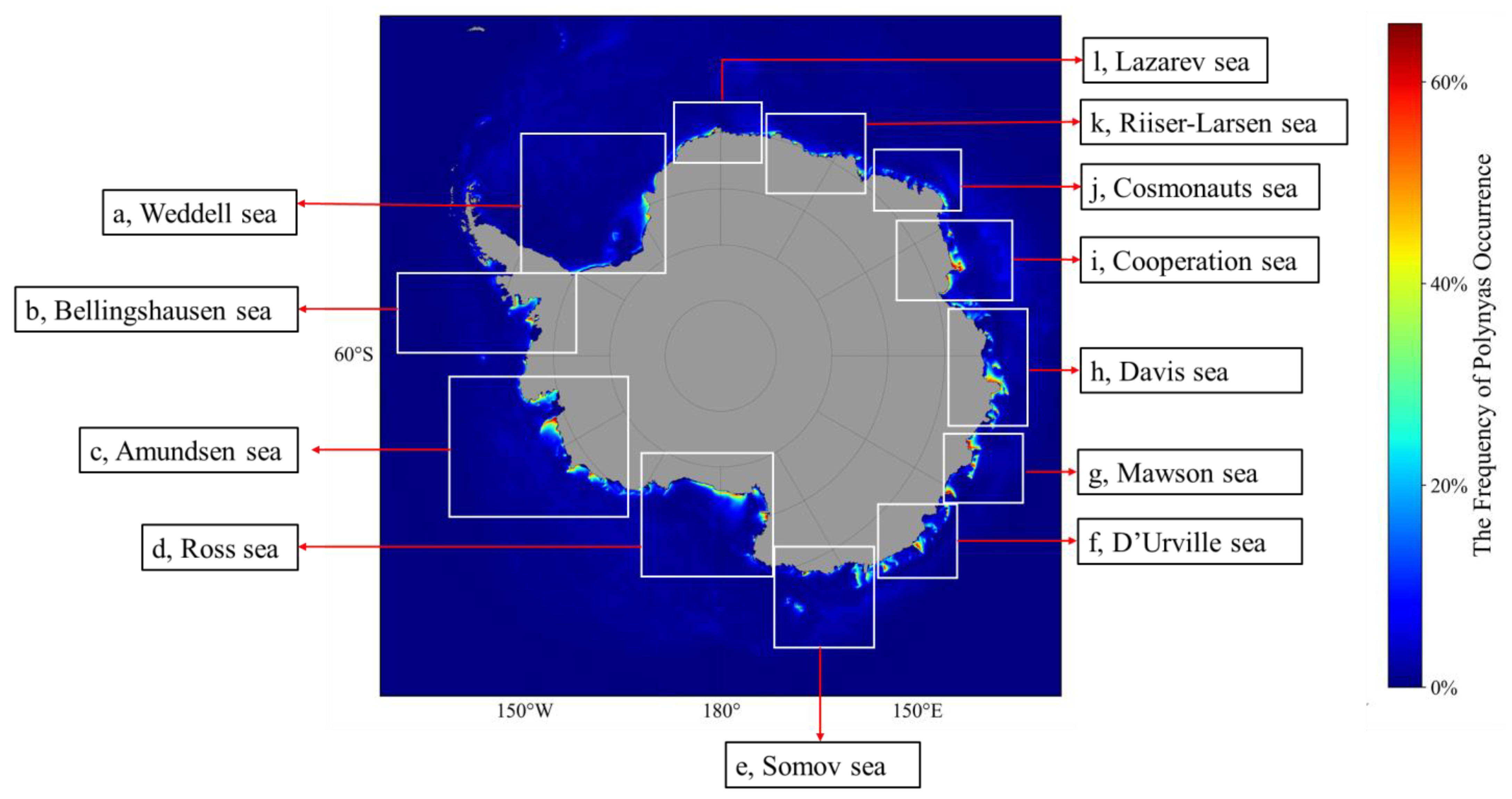
4.1. The Distribution of Polynyas in Arctic and Antarctic

Figure 4 illustrates the mean annual frequency of Arctic polynya occurrences over the decade spanning 2013–2022. This frequency is defined as the ratio of the number of days with polynya presence to the total number of days during this period. Thirteen regions characterized by concentrated polynya activity are delineated in Figure 4 by white rectangular markers. These regions are located in: (a) the Chukchi Sea; (b) the Beaufort Sea; (c) the Canadian Arctic Archipelago; (d) the Eastern coast of Davis Strait; (e) the NOW; (f) the Northeast Water polynya; (g) the region surrounding Svalbard; (h) the northern side of Franz Josef Land; (i) the Kara Sea; (j) Severnaya Zemlya; (k) the Laptev Sea; (l) the East Siberian Sea (m) the Okhotsk Sea. The results of Arctic polynyas are consistent with those obtained by Tamura and Ohshima [58].
The highest average annual occurrence frequency of Arctic polynyas, reaching up to 42%, is observed in the NOW polynya. This means that polynyas in this region can potentially occur for an average of 160 days per year. This region has been a major focus of previous studies [24,59], with studies primarily focusing on the variability of polynya characteristics and ice production processes in this area. From Figure 4, Arctic polynyas are predominantly distributed along the circum-Arctic coastal regions, exhibiting classic coastal polynya characteristics. Furthermore, some polynyas also occur in the mid-Arctic Ocean, with lower occurrence frequencies (<5%) corresponding to shorter durations (<15 days/year). These may represent transient sea ice fractures or enclosed areas formed by sea ice melting or wind/current [60]. The emergence of high-latitude polynyas in the mid-Arctic demands considerable attention.
We have classified these Antarctic polynyas into 12 sectors based on their geographical distribution in the Southern Ocean: (a) the Weddell Sea, (b) the Bellingshausen Sea, (c) the Amundsen Sea, (d) the Ross Sea, (e) the Somov Sea, (f) the D’Urville Sea, (g) the Mawson Sea, (h) the Davis Sea, (i) the Cooperation Sea, (j) the Cosmonauts Sea, (k) the Riiser-Larsen Sea, and (l) the Lazarev Sea. As shown in Figure 4, these sectors are marked with white rectangles, consistent with the classification used for the Arctic. Notably, each sector contains multiple individual polynyas.
Despite differences between the Antarctic and Arctic—the former being an ice-covered continent and the latter an ocean—the spatial distribution of polynyas in both regions exhibits remarkable similarities, with most polynyas forming along coastal margins. In the Antarctic, polynyas predominantly occur adjacent to the continent. As shown in Figure 5, the statistical analysis of isolated regions with occurrence rates exceeding 40% reveals that more than 20 Antarctic polynyas have an average annual occurrence frequency above 40%, while over 40 polynyas exceed 20%. The highest average annual occurrence frequencies are observed in three key regions: (c) the Amundsen Sea, (i) the Cooperation Sea, and (g) the Mawson Sea, where frequencies exceed 70%, corresponding to more than 255 days per year under open-ocean or thin-ice conditions. The results align with the distribution results of Antarctic polynyas, as reported by Lin et al. [9].

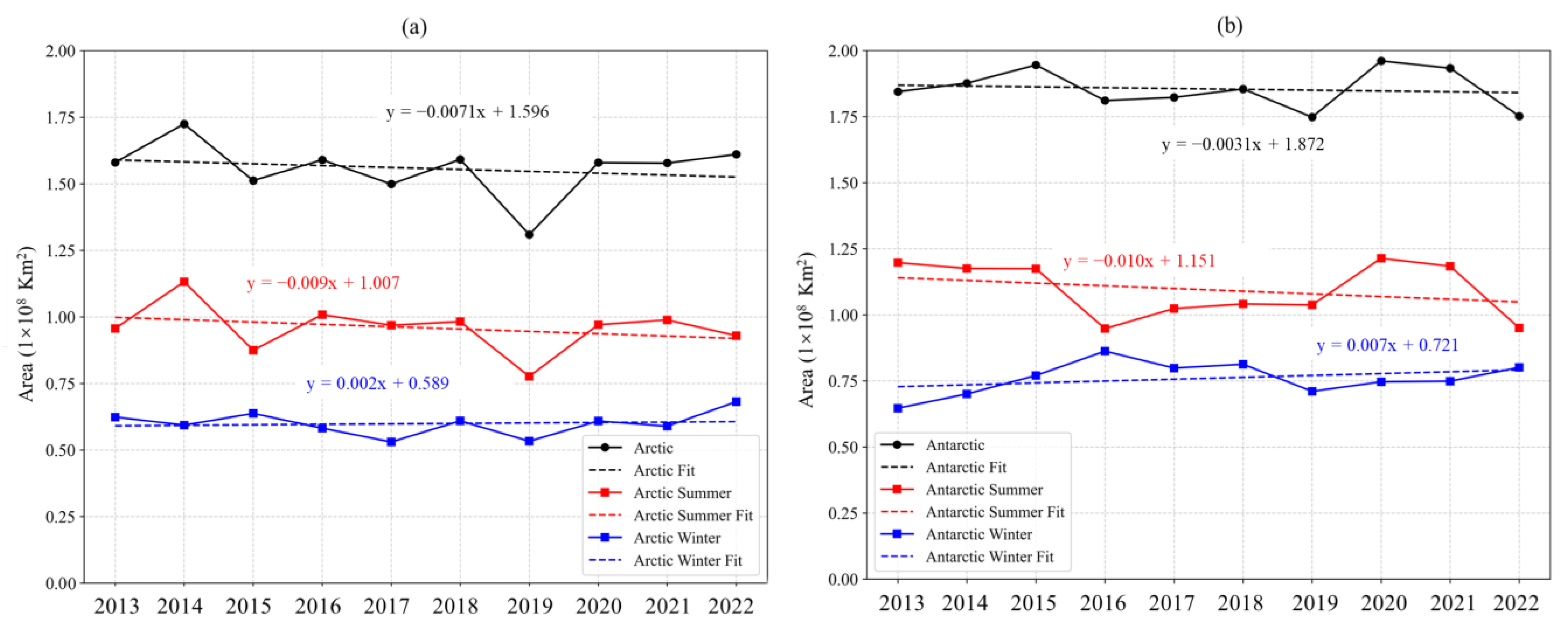
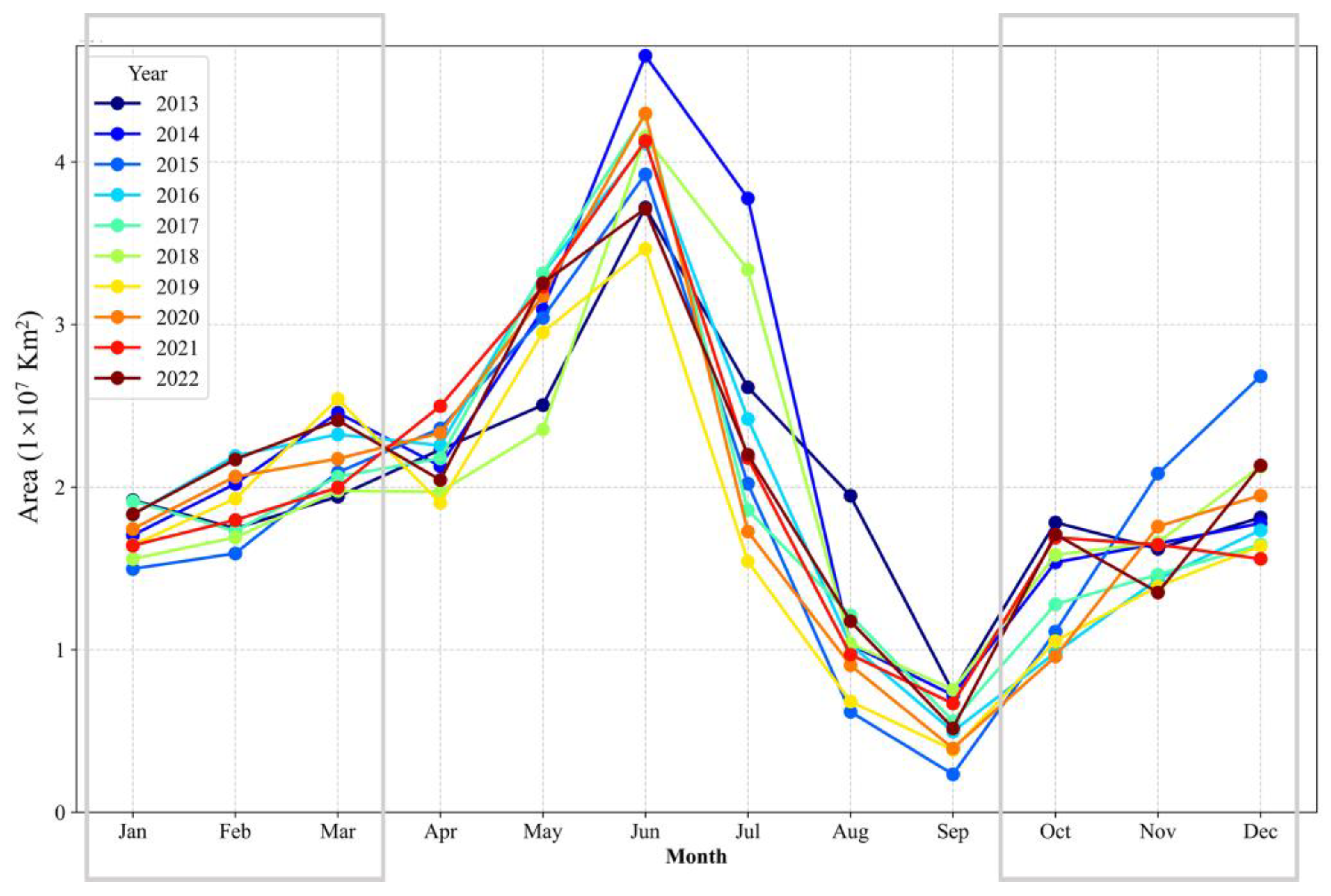
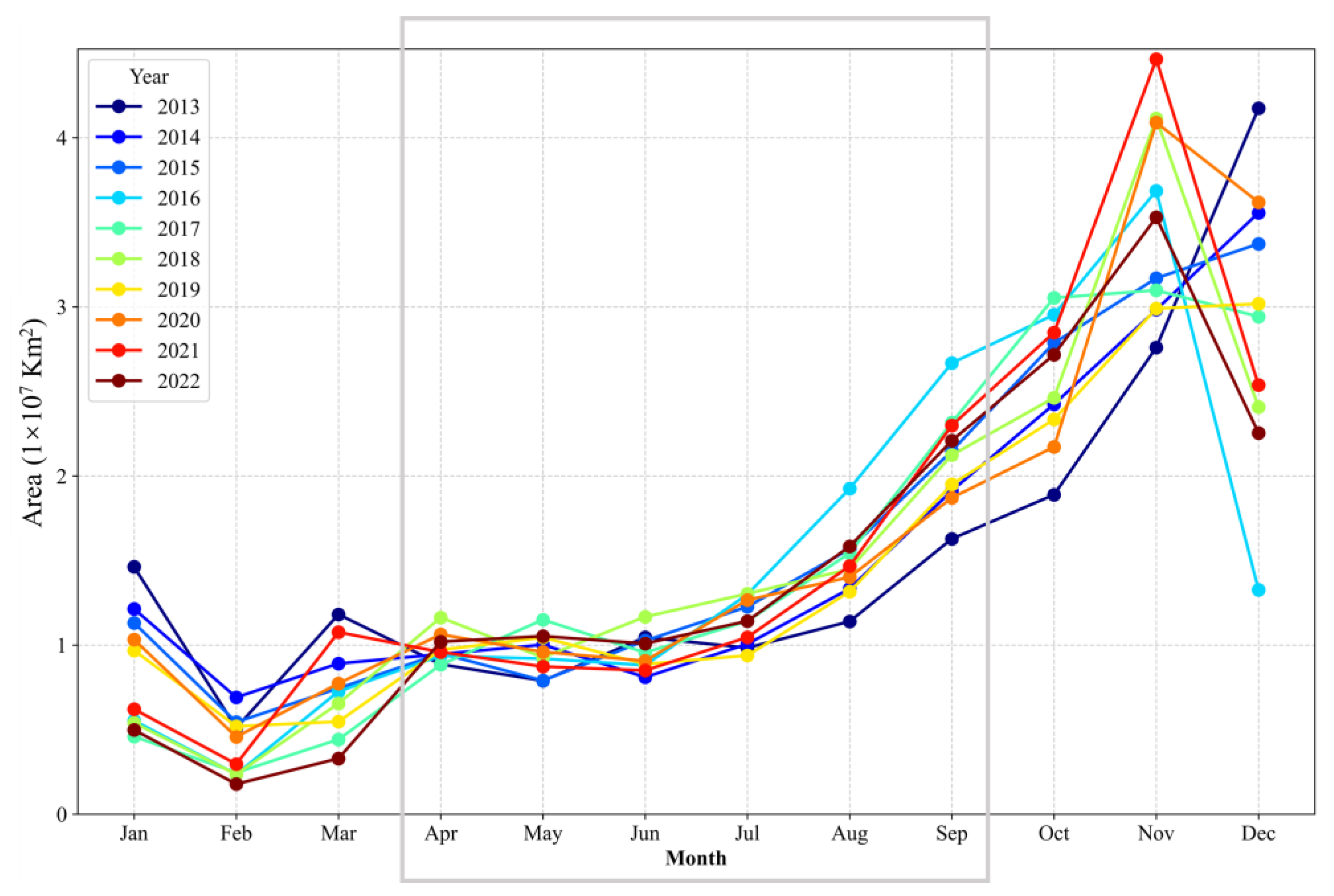
4.2. Decadal Changes of Polynyas in the Arctic and Antarctic

We use a linear correlation analysis on the occurrence frequency of Arctic and Antarctic polynyas from 2013 to 2022. The slope of the linear fit represents the average annual trend in polynya occurrence frequency, where a positive slope indicates an increasing trend and a negative slope signifies a decline over the past decade. Regions with correlation coefficients below 0.6 and p-value exceed 0.05 are excluded, as they exhibited no statistically significant interannual variability in polynya occurrence during the study period.
The spatial-temporal patterns of polynya occurrence frequency between 2013 and 2022 are clearly demonstrated in Figure 6. The analysis reveals that the spatial extent of Arctic polynyas is generally smaller than their Antarctic counterparts. The Arctic and Antarctic polynya occurrence frequencies show variations ranging from −3% to 3% (±3% means that the polynya occurrence frequency in that region increases or decreases by approximately 10 days per year, respectively) and with distinct regional differences. Specifically, increasing trends are observed in Chukchi Sea, and Fram Strait regions. And a significant decreasing trend is detected in the NOW region (as shown in Figure 6a1), while the occurrence frequencies of polynyas in other areas remain relatively stable or show no significant interannual variability. In addition, the Antarctic polynyas decrease in occurrence frequency are primarily concentrated in the Bellingshausen Sea, the D’Urville Sea, the Davis Sea, and the Cooperation Sea, and the other Antarctic regions demonstrate increasing trends. In Figure 6b1, we present the variation in polynya occurrence frequency in the Weddell Sea. The eastern side of the Weddell Sea exhibits an increasing trend, while the western side shows a decreasing trend.
Figure 7 illustrates the decadal variations in polynya area—encompassing annual, winter, and summer aggregates—from 2013 to 2022. Over this period, polynya areas in both the Arctic and Antarctic remained relatively stable. In the Antarctic, the annual total polynya area averaged approximately 1.86 × 10⁸ km2, with an interannual fluctuation of −3.1 × 10⁵ km2 per year and interannual rate of change below 0.01%. Similarly, the Arctic polynya area averaged around 1.59 × 10⁸ km2/y, exhibiting an interannual fluctuation of –7.1 × 10⁵ km2 per year. The area of polynyas in winter can better reflect the sea ice production [6,9,42]. In Figure 7, the blue dotted line denotes the variation in winter polynya area across both regions. Typically, the Arctic winter spans from October to March of the following year, whereas the Antarctic winter extends from April to September [16,40]. Both regions show a modest increase in winter polynya area, with average annual increments of 2 × 10⁵ km2/y in the Arctic and 7 × 10⁵ km2/y in the Antarctic. The total winter and summer polynya areas in the Arctic exhibited synchronous variation trends, while Antarctic data revealed distinct patterns: the winter polynya area peaked in 2016 then gradually declining, in contrast to the summer polynya area, which reached its minimum in the same year. These patterns likely reflect corresponding trends in Antarctic Sea ice, which experienced a significant increase until 2015 followed by a gradual decline. Consequently, the evolution of the Antarctic winter polynya area is consistent with the initial increase and subsequent decrease in Antarctic sea ice between 2013 and 2022 [61]. We therefore hypothesize that the polynya area is a critical indicator of future sea ice dynamics, particularly in the Antarctic region.
The development of polynyas, including their formation, expansion, and duration, is governed by a combination of factors, including solar insolation, temperature variations, wind patterns, ocean currents, and ice formation and melting [62,63]. Figure 8 and Figure 9 present the monthly variations in polynya area from 2013 to 2022 for the Arctic and Antarctic, respectively. The results indicate that Arctic polynyas reach their maximum extent in May and their minimum in September, whereas Antarctic polynyas peak in November and reach their lowest extent in February. In addition, the polynya area tends to increase during the winter months in both hemispheres.
The timing of minimum polynya extent coincides with the periods of minimum sea ice cover—September in the Arctic and February in the Antarctic. Interestingly, the maximum polynya area lags behind the maximum sea ice extent by approximately 1–2 months in both regions. This seasonal pattern reflects the interplay of thermodynamic and dynamic processes. In spring, rising solar insolation and ambient temperatures promote localized melting at the ice margins, increasing the extent of low-concentration sea ice and facilitating polynya formation and expansion. By summer, many polynyas either merge with the open ocean or exceed the threshold size for classification, leading to a rapid decline in their monitored area. As sea ice reaches its minimum extent, most coastal regions become ice-free, and the majority of polynyas disappear entirely.
In addition to seasonal drivers, offshore winds and ocean currents modulate polynya distribution and evolution by influencing both ice melting and refreezing processes [3]. The observed lag between maximum sea ice extent and peak polynya area highlights the delayed response of polynyas to the combined effects of heat-driven melting and atmospheric-oceanic interactions [64,65]. These findings provide key insights into the coupling between sea ice dynamics and regional climate.

4.3. Relationship Among Chlorophyll-a Concentration, Polynya Area and Environmental Parameters

Polynyas are critical regions for primary productivity, and polar phytoplankton. Chlorophyll-a concentration serves as a key indicator of marine biological activity, especially in relation to algal dynamics. Both polynya extent and chlorophyll-a concentration are closely linked to physical environmental parameters and are influenced by multiple interacting factors.
In this study, we analyzed chlorophyll-a concentration data derived from satellite remote sensing in polynya regions (available only during ice-free periods), alongside concurrent physical environmental variables, including sea surface temperature, 10 m wind speed, clear-sky direct solar radiation at the surface, and total cloud cover. All the data mentioned above are area-averaged values for the polynya regions. Our aim is to investigate the relationships among polynya area variability, chlorophyll-a concentration dynamics and the other environment parameters.
We focused on three representative polynya regions in the Arctic and Antarctic: (1) the Weddell Sea polynya (Antarctic), from 31 January to 16 February 2020; (2) the Beaufort Sea polynya (Arctic), from 1 April to 10 April 2020; and (3) NOW polynya, from 9 April to 19 April 2020. The corresponding results are presented in Figure 10. We selected three red-boxed regions in Figure 10—(a) polynyas in the southern Beaufort Gyre, (b) the NOW polynya, and (c) the Weddell Sea polynya—to analyze the relationships between polynya area, chlorophyll-a concentration, and environmental parameters.
Figure 10a illustrates the relationship among polynya area, chlorophyll-a concentration, and environmental parameters in the Beaufort Sea polynya. Based on statistical analysis of the correlations and p-values among various parameters in the region, we found that only the area of the polynya and wind speed exhibit a significant negative correlation, with a correlation coefficient (r) of −0.76 and a p-value of less than 0.02. This is primarily because the wind direction in this region is opposite to the expansion direction of the polynya (the polynya expands northward, while the wind blows from north to south). Therefore, during the lifecycle of this polynya, wind speed acts as a factor inhibiting its growth. This characteristic is similar to the phenomena observed by Montes-Hugo and Yuan in the Dumont d’Urville and Prydz Bay polynyas [2]. For other parameters, the p-values between polynya area and chlorophyll-a concentration are all greater than 0.05, indicating no significant correlation. The polynya area and chlorophyll-a concentration exhibit a weak positive correlation (r = 0.42), but the p-value is 0.26, indicating that the polynya area is not a dominant factor influencing chlorophyll-a concentration in this region. Further analysis of the correlations between other parameters and polynya area as well as chlorophyll-a concentration reveals that SST shows a slight positive correlation with polynya area (p = 0.11), while total cloud cover exhibits a slight negative correlation with polynya area (p = 0.13). Although these correlations are not significant, temperature and cloud cover characterize the intensity of solar radiation and can, to some extent, reflect changes in polynya area.
Figure 10b,c both demonstrate a significant positive correlation between polynya area and chlorophyll-a concentration. The correlation between the NOW polynya area and chlorophyll-a concentration is 0.73, with a p-value of 0.01, while the correlation between the Weddell Sea polynya area and chlorophyll-a concentration reaches 0.62, with a p-value of 0.01. The high correlation between polynya area and the average chlorophyll-a concentration indicates that polynyas provide critical habitats for these organisms. These results are consistent with the conclusion that polynyas are hotspots of biological activity [52,66]. However, other environmental variables in these two polynyas show no significant linear correlation with either polynya area or chlorophyll-a concentration (|r| < 0.4, p-values all greater than 0.05). This suggests that the formation of these polynyas is a complex process driven by the coupling of multiple factors. Using a single variable alone cannot adequately describe the changes in polynya area and chlorophyll-a concentration. In the future, more accurate data (e.g., in situ measurements) and more detailed oceanographic data (e.g., waves, and currents) will be needed to analyze the causes of changes in polynya area and chlorophyll-a concentration in this region.
From Figure 10, we observe a significant positive correlation between the area of the NOW and Weddell Sea polynyas and their respective chlorophyll-a concentrations. Figure 11 further examines this relationship, revealing that despite differences in geographic location, duration, and size, both polynyas exhibit consistent trends: chlorophyll-a concentration increases as the polynya expands and decreases as it contracts. This suggests that polynya size directly shapes the phytoplankton habitat, with its opening and closing influencing regional primary productivity.
Moreover, chlorophyll-a concentration in both polynyas responds more rapidly to area changes, with concentration variations exceeding those of polynya extent over short timescales. This discrepancy arises from the differing temporal scales of biological and physical processes [66]. As the opening and closing of polynyas regulate heat and material exchange between the ocean and atmosphere, thereby promoting or inhibiting marine primary production. The area of a polynya is a critical condition that must be met for algal growth. Phytoplankton biomass, reflected in chlorophyll-a concentration levels, responds almost immediately to the improved light availability, nutrient influx, and favorable temperatures following polynya formation, often leading to exponential growth within days [48]. In contrast, physical processes governing polynya dynamics, such as sea ice melting, heat exchange, wind forcing, and ocean currents, operate more gradually due to the thermal inertia of ice and large-scale ice dynamics [40]. While chlorophyll-a concentration and polynya area ultimately follow similar trends, the faster biological response likely explains the observed lag between changes in polynya area and chlorophyll-a concentration.

5. Conclusions

This study integrates SIC with SAR to map Arctic and Antarctic polynyas from 2013 to 2022. It examines the spatial distribution of polynyas in both polar regions, as well as their interannual and seasonal variability over the decade. Using reanalysis data, the study further explores the relationships between the area of classic polynyas and key environmental factors, as well as chlorophyll-a concentration.
Using SAR data in conjunction with SIC, this study determined the optimal SIC threshold for polynya extraction. A global SIC threshold of 75% is identified as the most effective for accurately delineating polynya boundaries through comparative analysis. Analysis of polynya occurrence frequencies from 2013 to 2022 revealed distinct regional patterns. In the Arctic, polynyas are primarily concentrated along coastal areas, with the NOW polynya exhibiting the highest occurrence frequency of approximately 42%, corresponding to about 160 days of open-water conditions per year. In the Antarctic, several regions showed occurrence frequencies exceeding 70%, indicating more than 255 days of open-water conditions annually.
Over the period from 2013 to 2022, polynya areas in both Arctic and Antarctic remained relatively stable. In Antarctic, the annual averaged polynya area approximately 1.86 × 10⁸ km2, with an interannual fluctuation of −3.1 × 10⁵ km2/y and interannual rate of change below 0.01%. Similarly, the Arctic polynya area averaged around 1.59 × 10⁸ km2/y, with an interannual fluctuation of −7.1 × 10⁵ km2/y. The total winter and summer polynya areas in the Arctic exhibited synchronous variation trends, while Antarctic data revealed distinct patterns: the winter polynya area peaked in 2016 then gradually declining, whereas the summer polynya area reached its minimum in the same year. The polynyas area in Arctic reached their maximum extent in May and their minimum in September, while Antarctic polynyas peaked in November and contracted to their smallest extent in February. In both hemispheres, polynya area generally increased during the winter months.
Correlation analysis of polynya area and key environmental variables in three typical Arctic and Antarctic polynyas reveals that polynya formation and development result from a complex interplay of multiple factors, no single variable can fully explain the variations in polynya extent. In addition, polynya areas in the NOW and Weddell Sea polynyas exhibit consistent trend with that of chlorophyll-a concentration, which highlights their critical role as habitats for primary productivity in polar regions. A causal relationship exists between polynya area and chlorophyll-a concentration, as the opening and closing of polynyas regulate heat and material exchange between the ocean and atmosphere, thereby promoting or inhibiting marine primary production [10,67].
This study revealed the spatiotemporal dynamics of Arctic and Antarctic polynyas and their bio-environmental associations using satellite remote sensing. Future research should integrate in-situ measurements with remote sensing to overcome 2D limitations and uncover how 3D thermohaline structures influence plankton migration and carbon transport. Coupling high-resolution regional climate and sea ice-ocean models can quantify the effects of wind, shear stress, and heat flux on polynya dynamics. Finally, advanced deep learning could enhance small-scale polynya detection using SAR and multispectral data, providing higher-resolution insights into polar dynamics.

Supplementary Materials

The following supporting information can be downloaded at: https://www.mdpi.com/article/10.3390/rs17071213/s1, Supplementary Materials: The other 17 SAR images used for polynya delineation.

Author Contributions

Conceptualization, K.Y.; methodology, K.Y.; software, K.Y.; validation, K.Y. and F.X.; formal analysis, M.Z. and F.X.; investigation, J.W.; data curation, H.L.; writing—original draft preparation, K.Y.; writing—review and editing, J.W.; visualization, J.W.; supervision, H.L.; funding acquisition, H.L. All authors have read and agreed to the published version of the manuscript.

Funding

This work was supported by the National Key R&D Program of China (No. 2022YFC3104904), the Fundamental Research Funds for the Central Universities, and supported by FY-3(03)-AS-11.10-ZT and FY-3(03)-AS-11.12-ZT.

Data Availability Statement

The original contributions presented in this study are included in the article/Supplementary Material. Further inquiries can be directed to the corresponding author.

Acknowledgments

The authors would like to thank the University of Bremen for providing sea ice concentration, the European Space Agency (ESA) for providing Sentinel-1 data and chlorophyll-a concentration data, and the ECMWF for providing ERA5 data.

Conflicts of Interest

The authors declare no conflicts of interest.

References

  1. Barber, D.G.; Massom, R.A. Chapter 1 The Role of Sea Ice in Arctic and Antarctic Polynyas. In Elsevier Oceanography Series; Elsevier: Amsterdam, The Netherlands, 2007; Volume 74, pp. 1–54. ISBN 978-0-444-52952-7. [Google Scholar]
  2. Montes-Hugo, M.A.; Yuan, X. Climate Patterns and Phytoplankton Dynamics in Antarctic Latent Heat Polynyas. J. Geophys. Res. Oceans 2012, 117, C05031. [Google Scholar] [CrossRef]
  3. Smith, S.D.; Muench, R.D.; Pease, C.H. Polynyas and Leads: An Overview of Physical Processes and Environment. J. Geophys. Res. Oceans 1990, 95, 9461–9479. [Google Scholar] [CrossRef]
  4. Bromwich, D.H.; Carrasco, J.F.; Liu, Z.; Tzeng, R. Hemispheric Atmospheric Variations and Oceanographic Impacts Associated with Katabatic Surges across the Ross Ice Shelf, Antarctica. J. Geophys. Res. Atmos. 1993, 98, 13045–13062. [Google Scholar] [CrossRef]
  5. Dokken, S.T.; Winsor, P.; Markus, T.; Askne, J.; Björk, G. ERS SAR Characterization of Coastal Polynyas in the Arctic and Comparison with SSM/I and Numerical Model Investigations. Remote Sens. Environ. 2002, 80, 321–335. [Google Scholar] [CrossRef]
  6. Nakata, K.; Ohshima, K.I.; Nihashi, S. Mapping of Active Frazil for Antarctic Coastal Polynyas, With an Estimation of Sea-Ice Production. Geophys. Res. Lett. 2021, 48, e2020GL091353. [Google Scholar] [CrossRef]
  7. Cheon, W.G.; Gordon, A.L. Open-Ocean Polynyas and Deep Convection in the Southern Ocean. Sci. Rep. 2019, 9, 6935. [Google Scholar] [CrossRef]
  8. Nakata, K.; Ohshima, K.I. Mapping of Active Frazil and Sea Ice Production in the Northern Hemisphere, with Comparison to the Southern Hemisphere. J. Geophys. Res. Ocean. 2022, 127, e2022JC018553. [Google Scholar] [CrossRef]
  9. Lin, Y.; Nakayama, Y.; Liang, K.; Huang, Y.; Chen, D.; Yang, Q. A Dataset of the Daily Edge of Each Polynya in the Antarctic. Sci. Data 2024, 11, 1006. [Google Scholar] [CrossRef]
  10. Arrigo, K.R.; Van Dijken, G.L. Phytoplankton Dynamics within 37 Antarctic Coastal Polynya Systems. J. Geophys. Res. Ocean. 2003, 108, 3271. [Google Scholar] [CrossRef]
  11. Murakami, K.; Nomura, D.; Hashida, G.; Nakaoka, S.; Kitade, Y.; Hirano, D.; Hirawake, T.; Ohshima, K.I. Strong Biological Carbon Uptake and Carbonate Chemistry Associated with Dense Shelf Water Outflows in the Cape Darnley Polynya, East Antarctica. Mar. Chem. 2020, 225, 103842. [Google Scholar] [CrossRef]
  12. Ohshima, K.I.; Nihashi, S.; Iwamoto, K. Global View of Sea-Ice Production in Polynyas and Its Linkage to Dense/Bottom Water Formation. Geosci. Lett. 2016, 3, 13. [Google Scholar] [CrossRef]
  13. Morales Maqueda, M.A.; Willmott, A.J.; Biggs, N.R.T. Polynya Dynamics: A Review of Observations and Modeling: Polynya Dynamics-Observations and Modeling. Rev. Geophys. 2004, 42, RG1004. [Google Scholar] [CrossRef]
  14. Jeong, H.; Lee, S.-S.; Park, H.-S.; Stewart, A.L. Future Changes in Antarctic Coastal Polynyas and Bottom Water Formation Simulated by a High-Resolution Coupled Model. Commun. Earth Environ. 2023, 4, 490. [Google Scholar] [CrossRef]
  15. Ohshima, K.I.; Fukamachi, Y.; Williams, G.D.; Nihashi, S.; Roquet, F.; Kitade, Y.; Tamura, T.; Hirano, D.; Herraiz-Borreguero, L.; Field, I.; et al. Antarctic Bottom Water Production by Intense Sea-Ice Formation in the Cape Darnley Polynya. Nat. Geosci. 2013, 6, 235–240. [Google Scholar] [CrossRef]
  16. Cornish, S.B.; Johnson, H.L.; Mallett, R.D.C.; Dörr, J.; Kostov, Y.; Richards, A.E. Rise and Fall of Sea Ice Production in the Arctic Ocean’s Ice Factories. Nat. Commun. 2022, 13, 7800. [Google Scholar] [CrossRef]
  17. Park, J.; Kuzminov, F.I.; Bailleul, B.; Yang, E.J.; Lee, S.; Falkowski, P.G.; Gorbunov, M.Y. Light Availability Rather than Fe Controls the Magnitude of Massive Phytoplankton Bloom in the Amundsen Sea Polynyas, Antarctica. Limnol. Oceanogr. 2017, 62, 2260–2276. [Google Scholar] [CrossRef]
  18. Dinniman, M.S.; St-Laurent, P.; Arrigo, K.R.; Hofmann, E.E.; Van Dijken, G.L. Sensitivity of the Relationship Between Antarctic Ice Shelves and Iron Supply to Projected Changes in the Atmospheric Forcing. J. Geophys. Res. Ocean. 2023, 128, e2022JC019210. [Google Scholar] [CrossRef]
  19. Kern, S.; Spreen, G.; Kaleschke, L.; De La Rosa, S.; Heygster, G. Polynya Signature Simulation Method Polynya Area in Comparison to AMSR-E 89GHz Sea-Ice Concentrations in the Ross Sea and off the Adélie Coast, Antarctica, for 2002–2005: First Results. Ann. Glaciol. 2007, 46, 409–418. [Google Scholar] [CrossRef]
  20. Heuzé, C.; Zhou, L.; Mohrmann, M.; Lemos, A. Spaceborne Infrared Imagery for Early Detection of Weddell Polynya Opening. Cryosphere 2021, 15, 3401–3421. [Google Scholar] [CrossRef]
  21. Liang, Z.; Pang, X.; Ji, Q.; Zhao, X.; Li, G.; Chen, Y. An Entropy-Weighted Network for Polar Sea Ice Open Lead Detection from Sentinel-1 SAR Images. IEEE Trans. Geosci. Remote Sens. 2022, 60, 4304714. [Google Scholar] [CrossRef]
  22. Yang, K.; Li, H.; Perrie, W.; Scharien, R.K.; Wu, J.; Zhang, M.; Xu, F. Fine Resolution Classification of New Ice, Young Ice, and First-Year Ice Based on Feature Selection from Gaofen-3 Quad-Polarization SAR. Remote Sens. 2023, 15, 2399. [Google Scholar] [CrossRef]
  23. Willmes, S.; Adams, S.; Schröder, D.; Heinemann, G. Spatio-Temporal Variability of Polynya Dynamics and Ice Production in the Laptev Sea between the Winters of 1979/80 and 2007/08. Polar Res. 2011, 30, 5971. [Google Scholar] [CrossRef]
  24. Preußer, A.; Heinemann, G.; Willmes, S.; Paul, S. Multi-Decadal Variability of Polynya Characteristics and Ice Production in the North Water Polynya by Means of Passive Microwave and Thermal Infrared Satellite Imagery. Remote Sens. 2015, 7, 15844–15867. [Google Scholar] [CrossRef]
  25. Collins, C.O.; Rogers, W.E.; Marchenko, A.; Babanin, A.V. In Situ Measurements of an Energetic Wave Event in the Arctic Marginal Ice Zone. Geophys. Res. Lett. 2015, 42, 1863–1870. [Google Scholar] [CrossRef]
  26. Gould, J.; Sloyan, B.; Visbeck, M. In Situ Ocean Observations. In International Geophysics; Elsevier: Amsterdam, The Netherlands, 2013; Volume 103, pp. 59–81. ISBN 978-0-12-391851-2. [Google Scholar]
  27. Adams, S.; Willmes, S.; Heinemann, G.; Rozman, P.; Timmermann, R.; Schröder, D. Evaluation of Simulated Sea-Ice Concentrations from Sea-Ice/Ocean Models Using Satellite Data and Polynya Classification Methods. Polar Res. 2011, 30, 7124. [Google Scholar] [CrossRef]
  28. Mohrmann, M.; Heuzé, C.; Swart, S. Southern Ocean Polynyas in CMIP6 Models. Cryosphere 2021, 15, 4281–4313. [Google Scholar] [CrossRef]
  29. Cooke, C.L.V.; Scott, K.A. Estimating Sea Ice Concentration From SAR: Training Convolutional Neural Networks with Passive Microwave Data. IEEE Trans. Geosci. Remote Sens. 2019, 57, 4735–4747. [Google Scholar] [CrossRef]
  30. Parera-Portell, J.A.; Ubach, R.; Gignac, C. An Improved Sea Ice Detection Algorithm Using MODIS: Application as a New European Sea Ice Extent Indicator. Cryosphere 2021, 15, 2803–2818. [Google Scholar] [CrossRef]
  31. Lin, Y.; Yang, Q.; Shi, Q.; Nakayama, Y.; Chen, D. A Volume-Conserved Approach to Estimating Sea-Ice Production in Antarctic Polynyas. Geophys. Res. Lett. 2023, 50, e2022GL101859. [Google Scholar] [CrossRef]
  32. Ivanova, N.; Johannessen, O.M.; Pedersen, L.T.; Tonboe, R.T. Retrieval of Arctic Sea Ice Parameters by Satellite Passive Microwave Sensors: A Comparison of Eleven Sea Ice Concentration Algorithms. IEEE Trans. Geosci. Remote Sens. 2014, 52, 7233–7246. [Google Scholar] [CrossRef]
  33. Wu, S.; Shi, L.; Zou, B.; Zeng, T.; Dong, Z.; Lu, D. Daily Sea Ice Concentration Product over Polar Regions Based on Brightness Temperature Data from the HY-2B SMR Sensor. Remote Sens. 2023, 15, 1692. [Google Scholar] [CrossRef]
  34. Cavalieri, D.J.; Gloersen, P.; Campbell, W.J. Determination of Sea Ice Parameters with the NIMBUS 7 SMMR. J. Geophys. Res. Atmos. 1984, 89, 5355–5369. [Google Scholar] [CrossRef]
  35. Kwok, R. Satellite Remote Sensing of Sea-Ice Thickness and Kinematics: A Review. J. Glaciol. 2010, 56, 1129–1140. [Google Scholar] [CrossRef]
  36. Huntemann, M.; Heygster, G.; Kaleschke, L.; Krumpen, T.; Mäkynen, M.; Drusch, M. Empirical Sea Ice Thickness Retrieval during the Freeze-up Period from SMOS High Incident Angle Observations. Cryosphere 2014, 8, 439–451. [Google Scholar] [CrossRef]
  37. Ricker, R.; Hendricks, S.; Kaleschke, L.; Tian-Kunze, X.; King, J.; Haas, C. A Weekly Arctic Sea-Ice Thickness Data Record from Merged CryoSat-2 and SMOS Satellite Data. Cryosphere 2017, 11, 1607–1623. [Google Scholar] [CrossRef]
  38. Yan, Q.; Huang, W.; Moloney, C. Neural Networks Based Sea Ice Detection and Concentration Retrieval From GNSS-R Delay-Doppler Maps. IEEE J. Sel. Top. Appl. Earth Obs. Remote Sens. 2017, 10, 3789–3798. [Google Scholar] [CrossRef]
  39. Yan, Q.; Huang, W. Sea Ice Thickness Measurement Using Spaceborne GNSS-R: First Results With TechDemoSat-1 Data. IEEE J. Sel. Top. Appl. Earth Obs. Remote Sens. 2020, 13, 577–587. [Google Scholar] [CrossRef]
  40. Golledge, N.R.; Keller, E.D.; Gossart, A.; Malyarenko, A.; Bahamondes-Dominguez, A.; Krapp, M.; Jendersie, S.; Lowry, D.P.; Alevropoulos-Borrill, A.; Notz, D. Antarctic Coastal Polynyas in the Global Climate System. Nat. Rev. Earth Environ. 2025, 6, 126–139. [Google Scholar] [CrossRef]
  41. Winsor, P.; Björk, G. Polynya Activity in the Arctic Ocean from 1958 to 1997. J. Geophys. Res. Ocean. 2000, 105, 8789–8803. [Google Scholar] [CrossRef]
  42. Tamura, T.; Ohshima, K.I. Mapping of Sea Ice Production in the Arctic Coastal Polynyas. J. Geophys. Res. Ocean. 2011, 116, C07030. [Google Scholar] [CrossRef]
  43. Dai, L.; Xie, H.; Ackley, S.F.; Mestas-Nuñez, A.M. Ice Production in Ross Ice Shelf Polynyas during 2017–2018 from Sentinel–1 SAR Images. Remote Sens. 2020, 12, 1484. [Google Scholar] [CrossRef]
  44. Nihashi, S.; Ohshima, K.I.; Tamura, T. Sea-Ice Production in Antarctic Coastal Polynyas Estimated From AMSR2 Data and Its Validation Using AMSR-E and SSM/I-SSMIS Data. IEEE J. Sel. Top. Appl. Earth Obs. Remote Sens. 2017, 10, 3912–3922. [Google Scholar] [CrossRef]
  45. Arrigo, K.R.; Van Dijken, G.L.; Strong, A.L. Environmental Controls of Marine Productivity Hot Spots around A Ntarctica. J. Geophys. Res. Ocean. 2015, 120, 5545–5565. [Google Scholar] [CrossRef]
  46. Berg, A.; Eriksson, L.E.B. SAR Algorithm for Sea Ice Concentration—Evaluation for the Baltic Sea. IEEE Geosci. Remote Sens. Lett. 2012, 9, 938–942. [Google Scholar] [CrossRef]
  47. Kwok, R.; Rothrock, D.A. Decline in Arctic Sea Ice Thickness from Submarine and ICESat Records: 1958–2008. Geophys. Res. Lett. 2009, 36, L15501. [Google Scholar] [CrossRef]
  48. Karvonen, J.; Cheng, B.; Vihma, T.; Arkett, M.; Carrieres, T. A Method for Sea Ice Thickness and Concentration Analysis Based on SAR Data and a Thermodynamic Model. Cryosphere 2012, 6, 1507–1526. [Google Scholar] [CrossRef]
  49. Smedsrud, L.H.; Halvorsen, M.H.; Stroeve, J.C.; Zhang, R.; Kloster, K. Fram Strait Sea Ice Export Variability and September Arctic Sea Ice Extent over the Last 80 Years. Cryosphere 2017, 11, 65–79. [Google Scholar] [CrossRef]
  50. Massom, R.A.; Harris, P.T.; Michael, K.J.; Potter, M.J. The Distribution and Formative Processes of Latent-Heat Polynyas in East Antarctica. Ann. Glaciol. 1998, 27, 420–426. [Google Scholar] [CrossRef]
  51. Sathyendranath, S.; Brewin, R.; Brockmann, C.; Brotas, V.; Calton, B.; Chuprin, A.; Cipollini, P.; Couto, A.; Dingle, J.; Doerffer, R.; et al. An Ocean-Colour Time Series for Use in Climate Studies: The Experience of the Ocean-Colour Climate Change Initiative (OC-CCI). Sensors 2019, 19, 4285. [Google Scholar] [CrossRef]
  52. Jiang, N.; Zhang, Z.; Zhang, R.; Wang, C.; Zhou, M. The Connection of Phytoplankton Biomass in the Marguerite Bay Polynya of the Western Antarctic Peninsula to the Southern Annular Mode. Acta Oceanol. Sin. 2024, 43, 35–47. [Google Scholar] [CrossRef]
  53. Williams, W.J.; Carmack, E.C.; Ingram, R.G. Chapter 2 Physical Oceanography of Polynyas. In Elsevier Oceanography Series; Elsevier: Amsterdam, The Netherlands, 2007; Volume 74, pp. 55–85. ISBN 978-0-444-52952-7. [Google Scholar]
  54. Barber, D.; Marsden, R.; Minnett, P.; Ingram, G.; Fortier, L. Physical Processes within the North Water (NOW) Polynya. Atmos.-Ocean 2001, 39, 163–166. [Google Scholar] [CrossRef]
  55. Park, J.; Kim, H.-C.; Jo, Y.-H.; Kidwell, A.; Hwang, J. Multi-Temporal Variation of the Ross Sea Polynya in Response to Climate Forcings. Polar Res. 2018, 37, 1444891. [Google Scholar] [CrossRef]
  56. Freeman, H. On the Encoding of Arbitrary Geometric Configurations. IEEE Trans. Electron. Comput. 1961, EC-10, 260–268. [Google Scholar] [CrossRef]
  57. Strong, C.; Rigor, I.G. Arctic Marginal Ice Zone Trending Wider in Summer and Narrower in Winter. Geophys. Res. Lett. 2013, 40, 4864–4868. [Google Scholar] [CrossRef]
  58. Tamura, T.; Ohshima, K.I.; Nihashi, S. Mapping of Sea Ice Production for Antarctic Coastal Polynyas: Mapping of Sea Ice Production. Geophys. Res. Lett. 2008, 35, L07606. [Google Scholar] [CrossRef]
  59. Ren, H.; Shokr, M.; Li, X.; Zhang, Z.; Hui, F.; Cheng, X. Estimation of Sea Ice Production in the North Water Polynya Based on Ice Arch Duration in Winter During 2006–2019. J. Geophys. Res. Ocean. 2022, 127, e2022JC018764. [Google Scholar] [CrossRef]
  60. Narayanan, A.; Roquet, F.; Gille, S.T.; Gülk, B.; Mazloff, M.R.; Silvano, A.; Naveira Garabato, A.C. Ekman-Driven Salt Transport as a Key Mechanism for Open-Ocean Polynya Formation at Maud Rise. Sci. Adv. 2024, 10, eadj0777. [Google Scholar] [CrossRef]
  61. Rackow, T.; Danilov, S.; Goessling, H.F.; Hellmer, H.H.; Sein, D.V.; Semmler, T.; Sidorenko, D.; Jung, T. Delayed Antarctic Sea-Ice Decline in High-Resolution Climate Change Simulations. Nat. Commun. 2022, 13, 637. [Google Scholar] [CrossRef]
  62. Smedsrud, L.H.; Sirevaag, A.; Kloster, K.; Sorteberg, A.; Sandven, S. Recent Wind Driven High Sea Ice Area Export in the Fram Strait Contributes to Arctic Sea Ice Decline. Cryosphere 2011, 5, 821–829. [Google Scholar] [CrossRef]
  63. Asplin, M.G.; Scharien, R.; Else, B.; Howell, S.; Barber, D.G.; Papakyriakou, T.; Prinsenberg, S. Implications of Fractured Arctic Perennial Ice Cover on Thermodynamic and Dynamic Sea Ice Processes. J. Geophys. Res. Ocean. 2014, 119, 2327–2343. [Google Scholar] [CrossRef]
  64. Goosse, H.; Allende Contador, S.; Bitz, C.M.; Blanchard-Wrigglesworth, E.; Eayrs, C.; Fichefet, T.; Himmich, K.; Huot, P.-V.; Klein, F.; Marchi, S.; et al. Modulation of the Seasonal Cycle of the Antarctic Sea Ice Extent by Sea Ice Processes and Feedbacks with the Ocean and the Atmosphere. Cryosphere 2023, 17, 407–425. [Google Scholar] [CrossRef]
  65. Aoki, S.; Takahashi, T.; Yamazaki, K.; Hirano, D.; Ono, K.; Kusahara, K.; Tamura, T.; Williams, G.D. Warm Surface Waters Increase Antarctic Ice Shelf Melt and Delay Dense Water Formation. Commun. Earth Environ. 2022, 3, 142. [Google Scholar] [CrossRef]
  66. Ardyna, M.; Arrigo, K.R. Phytoplankton Dynamics in a Changing Arctic Ocean. Nat. Clim. Chang. 2020, 10, 892–903. [Google Scholar] [CrossRef]
  67. Moreau, S.; Lannuzel, D.; Janssens, J.; Arroyo, M.C.; Corkill, M.; Cougnon, E.; Genovese, C.; Legresy, B.; Lenton, A.; Puigcorbé, V.; et al. Sea Ice Meltwater and Circumpolar Deep Water Drive Contrasting Productivity in Three Antarctic Polynyas. J. Geophys. Res. Ocean. 2019, 124, 2943–2968. [Google Scholar] [CrossRef]
Figure 1. The polynyas in SAR images and SIC. (a1) is the SAR HH intensity of Arctic costal polynya. (b1) is the SAR HH intensity of Arctic open-ocean polynya. (c1) is the SAR HH intensity of Antarctic polynya. In the (a2,b2,c2), SIC is added on the SAR images. The yellow boundaries are polynyas by visual interpretation in (a2,b2,c2). The red points are SIC < 75 and the blue points are SIC > = 75. The light green areas represent land. The names of the islands are labeled on each map.
Remotesensing 17 01213 g001
Figure 2. Polynyas’ extent and area differences at various SIC thresholds. The left and right vertical axes denote area difference and polynyas extent, respectively. Both parameters are with unit km2. The blue line is polynyas’ area from SAR images, the red line represents polynyas’ area in different sic thresholds. The green rectangles highlight the differences between polynyas’ areas derived from SAR images and those identified at various SIC thresholds. (a) represents the largest polynya (upper of land) shown in Figure 1a1, (b) corresponds to the polynya area depicted in Figure 1b2, and (c) corresponds to the polynya area illustrated in Figure 1c2.
Remotesensing 17 01213 g002
Figure 3. Extracting polynyas from SIC. (a1,a2): the distribution of SIC for Arctic and Antarctic. (b1,b2): the binarized SIC distribution. (c1,c2): the isolated open water regions. (d1,d2): the final extracted polynyas after area filtering.
Remotesensing 17 01213 g003
Figure 4. The occurrence frequency of polynyas in Arctic. White rectangles are the main distribution regions of Arctic polynyas. The colormap represents the frequency of polynya occurrence. It means the number of days of polynya occurrence in a decade divided by the total number of days in a decade.
Remotesensing 17 01213 g004
Figure 5. The occurrence frequency of polynyas in Antarctic. The white rectangles are the main distribution regions of Antarctic polynyas. The colormap represents the frequency of polynyas’ occurrence.
Remotesensing 17 01213 g005
Figure 6. The average annual rate of change in the occurrence frequency of polynyas in Arctic and Antarctic from 2013 to 2022. (a) shows the variation in the occurrence rate of polynyas in the Arctic region, with (a1) being a zoomed-in view of the NOW area. (b) illustrates the variation in the occurrence rate of polynyas in the Antarctic region, with (b1) providing a zoomed-in view of the Weddell Sea area.
Remotesensing 17 01213 g006
Figure 7. (a) shows the annual variations of the total polynya area, winter months total area, and summer months total area in the Antarctic from 2013 to 2022 (Antarctic winter spans from April to September, and summer spans from October to March of the following year). (b) illustrates the annual variations of the total polynya area, winter months total area, and summer months total area in the Arctic (Arctic winter spans from October to March of the following year, and summer spans from April to September). The annual variations of the total polynya area are represented by black dots, while red dots and blue dots represent winter and summer, respectively. Dashed lines and equations in different colors correspond to the linear regression results for different seasons.
Remotesensing 17 01213 g007
Figure 8. Monthly Distribution of the Arctic polynya area (2013–2022). The dot lines in different colors represent different years, and the gray rectangles indicate the winter months (from October to March of the following year).
Remotesensing 17 01213 g008
Figure 9. Monthly distribution of Antarctic polynya area (2013–2022). The dots lines in different colors represent different years, and the gray rectangles indicate the winter months (from April to September).
Remotesensing 17 01213 g009
Figure 10. Relationships among polynya area, chlorophyll-a concentration (Chl-a), and environmental parameters. The left panel of Figure 10 shows the geographical locations of the study regions (the background is the occurrences frequency of polynyas)—Beaufort Sea polynya, NOW polynya, and Weddell Sea polynya—marked with red boxes and arrows indicating their positions and correspondences. Panels (ac) present the correlations between these parameters in the respective regions, along with their associated p-values. Grid cells with p-values below 0.05 are highlighted in red, indicating statistically significant relationships, whereas those with p-values above 0.05 are highlighted in blue, denoting non-significant trends.
Remotesensing 17 01213 g010
Figure 11. Distribution of polynya area and chlorophyll-a concentration (chla) in the NOW polynya (a) and Weddell Sea polynya (b). The blue line represents the temporal variation of polynya area, while the red line indicates the mean chlorophyll-a concentration changes in this region.
Remotesensing 17 01213 g011
Disclaimer/Publisher’s Note: The statements, opinions and data contained in all publications are solely those of the individual author(s) and contributor(s) and not of MDPI and/or the editor(s). MDPI and/or the editor(s) disclaim responsibility for any injury to people or property resulting from any ideas, methods, instructions or products referred to in the content.

