Temporal–Spatial Partial Differential Equation Modeling of Land Cover Dynamics via Satellite Image Time Series and Sparse Regression

Abstract

Land cover dynamics play a critical role in understanding environmental changes, but accurately modeling these dynamics remains a challenge due to the complex interactions between temporal and spatial factors. In this study, we propose a novel temporal–spatial partial differential equation (TS-PDE) modeling method combining sparse regression to uncover the governing equations behind long-term satellite image time series. By integrating temporal and spatial differential terms, the TS-PDE framework captures the intricate interactivity of these factors, overcoming the limitations of traditional pixel-wise prediction methods. Our approach leverages $1\times 1$ convolutional kernels within a convolutional neural network (CNN) solver to approximate derivatives, enabling the discovery of interpretable equations that generalize across temporal–spatial domains. Using MODIS and Planet satellite data, we demonstrate the effectiveness of the TS-PDE method in predicting the value of the normalized difference vegetation index (NDVI) and interpreting the physical significance of the derived equations. The numerical results show that the model achieves good performance, with mean structural similarity index (SSIM) values exceeding 0.82, mean peak signal-to-noise ratio (PSNR) values ranging from 28.5 to 32.8, and mean mean squared error (MSE) values approximating $9\times {10}^{-4}$ for low-resolution MODIS images. For high-resolution Planet images, this study emphasizes the efficacy of TS-PDE in terms of PSNR, SSIM, and MSE metrics, with all datasets exhibiting an average SSIM value of over 0.81, an average PSNR maximum of 30.9, and an average MSE of less than 0.0042. The experimental findings demonstrate the capability of TS-PDE in deriving governing equations and providing effective predictions for the regional-scale dynamics of these time series images. The findings of this study provide potential insights into the mathematical modeling of land cover dynamics.

1. Introduction

Land cover modeling plays a critical role in understanding and managing Earth’s surface dynamics, with applications ranging from agricultural planning to climate change mitigation. Traditional approaches, such as cellular automata (CA) [1,2], CLUE [3], and stochastic element augmentation [4], have laid important foundations for this field. However, these approaches often struggle to capture the full complexity of spatiotemporal processes. Methods such as deep neural networks (DNNs) [5,6,7] and convolutional neural networks (CNNs) [8] often rely on data-driven methods, which face several limitations, including over-reliance on training data, limited spatiotemporal transferability and generalization, a lack of interpretability regarding underlying physical processes, and challenges in balancing overfitting on linear relationships with underfitting on complex nonlinear relationships.

Partial differential equations (PDEs) have emerged as a powerful tool for modeling spatiotemporal processes, offering a balance between physical interpretability and mathematical rigor. PDEs are frequently used to explicitly describe the laws governing dynamic systems in various fields of natural sciences and are of fundamental significance in many disciplines and engineering applications. For instance, the Navier–Stokes equation is used to describe the velocity and pressure distribution of a fluid [9], the heat conduction equation describes the distribution of temperature inside an object over time and space [10], and the wave equation and elasticity equation can be used to model the vibration behavior of buildings, bridges, and other structures [11]. These PDEs were initially constructed based on observed phenomena and the empirical understanding of the problem by scientists and showed that temporal derivatives can describe the evolution of variables along the direction of time while spatial derivatives can be regarded as variations in different regions of location. Subsequently, a correlation model is mathematically analyzed or numerically approximated to capture the system’s evolution.

AI for Science, a new research paradigm that integrates artificial intelligence (AI) methodologies into scientific discovery, brings tremendous promise for various disciplines due to a series of breakthroughs in deep learning and big data science. Scholars have begun to shift their focus from purely theoretical derivation to machine-based computing. Accordingly, data-driven equation discovery has become a research hotspot. One of the most typical methods is PDE-FIND [12], which discusses in detail how to discover partial differential equations from data. To achieve this, a library of candidate functions is constructed, consisting of all the relevant terms to be determined. Then, a sparse regression algorithm is used to select a small number of appropriate terms from the library and obtain their corresponding coefficients. Chen et al. [13] proposed a more robust deep learning symbolic genetic algorithm (SGA-PDE) that uses symbolic mathematics to discover free-form equations, thereby realizing the self-mining of governing equations from data. At the same time, scholars are committed to exploring the use of neural networks to characterize partial differential equations. Physics-informed neural networks (PINNs) [14,15,16] are proposed to approximate the solution of an equation while satisfying physical constraints, even when some coefficients are unknown. This approach is useful when the form of the right-hand term of the equation is known but not all coefficients are known. The unknown system can then be solved. Long et al. [17,18] proposed a data-driven feedforward neural network, named PDE-Net, to approximate the right-hand term of equations of unknown form. PDE-Net can be used to construct a system that approximates the partial differential equation and predicts its solution for a long time. However, these AI-driven PDE discovery frameworks focus on low-dimensional systems or simplified models that do not effectively scale to high-dimensional real-world problems, such as land cover dynamics. Addressing these limitations requires a more holistic approach that combines the strengths of data-driven learning with physical modeling principles.

The rapid advances of data-driven modeling methods have brought about a technological change in the way that partial differential equations are discovered. This change makes it possible to explore land cover dynamical systems from remotely sensed data, and the large volume of data just characterize the remote sensing discipline. Remote sensing images are the “photographs” of the Earth’s surface. The Earth’s surface can be considered as a complex giant dynamical system, but it is highly challenging to obtain a concise yet precise description of its internal laws under non-ideal conditions through mathematical derivation or experience. Therefore, data-driven methods gain more importance and are more suitable for extracting the main control equations of land cover dynamics.

There are many features regarding the description of land cover, and the normalized difference vegetation index (NDVI) is a comprehensive and representative one. The NDVI is a commonly used indicator for monitoring vegetation cover and growth patterns in various ecological, agricultural, and climate change studies. Concretely, the NDVI has been employed in diverse applications such as drought conditions monitoring [19,20], agricultural production predicting [21], land cover classification [22,23], etc. Therefore, continuous and accurate NDVI time series data are crucial for understanding vegetation dynamics and their response to land surface environmental changes. However, various factors often cause NDVI time series to be incomplete or noisy, requiring reconstruction efforts.

A range of methods have been developed for NDVI time series reconstruction or prediction, such as an autoregressive integrated moving average model combined with climatic data [24] and the Holt–Winters model in high- and low-vegetation regions [25]. However, these methods usually assume that NDVI time series exhibit linearity and smoothness, but they often fail to effectively capture the nonlinearities and irregularities hidden in NDVI time series during the forecasting process [26].

In recent years, more advanced machine learning and deep learning methods have been adopted to improve the accuracy of NDVI prediction. Tong et al. [27] introduced a pixel space gap-filling approach for soil moisture estimation on the Tibetan Plateau based on machine learning and geostatistics. In contrast to traditional statistical prediction techniques, machine learning methods excel at capturing nonlinear relationships between dependent and independent variables through extensive training, effectively addressing intricate prediction challenges posed by noisy data [28]. Roy et al. [29] employed four supervised machine learning algorithms—support vector machine regression (SVR), random forests (RFs), linear regression, and polynomial regression—to forecast NDVI data. Their findings revealed that the random forest and linear regression methods achieved superior prediction accuracy. However, it was also observed that these methods exhibited a certain sensitivity to mutations. Gao et al. [30] established a new NDVI prediction model by combining time series decomposition (TSD), a CNN, and long short-term memory (LSTM), called TSD-CNN-LSTM; Cui et al. [31] proposed SF-CNN, a new NDVI prediction model that combines a CNN and historical data statistical features. However, the majority of these methodologies employ temporal features and deep learning to improve prediction accuracy, yet they neglect to consider the spatial dependence of vegetation status. To augment spatial dependency, Xu et al. [32] captured long-range dependencies of NDVI time series by combining a non-local attention module and spatial autocorrelation modeling based on the local Moran index to learn spatial dependence, where a convolutional LSTM network (ConvLSTM) with spatial autocorrelation and non-local attention modules (ConvLSTM-SAC-NL) is proposed. Theoretically, the ConvLSTM-SAC-NL method improves the spatial dependence, but it still has some shortcomings in long-term prediction. How to integrate the spatial dependence of the surface state while achieving long-term prediction remains an unsolved issue. Moreover, there is still the question of how to explicitly interpret or to find the physical meaning behind these deep learning models.

Based on the above considerations, in this paper, we propose a temporal–spatial partial differential equation modeling (TS-PDE) method for land cover dynamics. TS-PDE can discover the governing equations behind long-term satellite image time series and establish the corresponding land cover dynamic system. Since the computation of the spatial partial derivative term involves spatial neighborhood information, it therefore has neighborhood recursion capabilities. By introducing temporal and spatial differential terms into the equations, the TS-PDE method captures the interactions between temporal changes and spatial patterns, which are often intertwined in land cover dynamics. This approach demonstrates the advantage of focusing on spatial dependence and temporal features during the prediction of full images compared to conventional methods as it integrates the contextual information from neighboring pixels and temporal trends across the image series. In other words, the discovered equations not only describe the local changes at individual pixels but also generalize the underlying rules governing the entire temporal–spatial domain of the training images. This generalization capability allows the equations to represent the common patterns and dynamics shared across the study area, making them applicable to broader spatial and temporal contexts.

The remainder of this paper is organized as follows: Section 2 introduces the two datasets used for experiments and details the proposed TS-PDE method. Section 3 presents the experimental results by showing the discovered equations and quantitatively evaluating the prediction performance of these equations. Section 4 discusses the physical significance, limitations, and future work of TS-PDE. Finally, conclusions are given in Section 5.

2. Materials and Methods

2.1. Research Data

The NDVI is a widely recognized and extensively used vegetation index in remote sensing. It exploits the unique spectral characteristics of vegetation, specifically the strong reflection of near-infrared (NIR) light and the significant absorption of red light by chlorophyll. The NDVI is calculated as the normalized difference between the reflectance values of the NIR and red bands, providing a quantitative measure of vegetation health and vigor:

$$\mathrm{NDVI}={\displaystyle \frac{\mathrm{NIR}-\mathrm{Red}}{\mathrm{NIR}+\mathrm{Red}}}$$

(1)

The NDVI ranges from $-1$ to 1, where higher values typically indicate healthier and denser vegetation while lower or negative values suggest sparse vegetation, bare soil, or other non-vegetative surfaces.

The NDVI serves as a critical parameter for assessing vegetation health, growth stages, and coverage. It is widely applied in precision agriculture, forestry, and ecological research, offering valuable insights into crop health, stress detection, and land use changes. Furthermore, its integration with modern remote sensing technologies has enhanced its utility in addressing global challenges such as food security, biodiversity conservation, and sustainable land management.

In summary, the NDVI provides a reliable and interpretable measure of vegetation status, contributing significantly to advancements in precision agriculture, ecological studies, and environmental monitoring. Moreover, the NDVI is a univariate index rather than the multiple spectral bands of raw satellite images, which helps us to concentrate on the modeling methodology itself without concerns about the relation among different variables. Therefore, this study employs NDVI data to validate the feasibility and accuracy of the proposed model. Two datasets with different spatial and temporal resolutions, the MODIS dataset and Planet dataset, are used to demonstrate the robustness and adaptivity of the proposed TS-PDE method.

2.1.1. MODIS Dataset

Moderate-resolution imaging spectroradiometer (MODIS) data are a typical satellite image data source that lasts for decades and is widely used by many large-scale environmental applications. The dataset used in this study comprises the MOD13Q1 NDVI data products (orbit number H26V05), which have a spatial resolution of 250 m and a temporal resolution of 16 days. This dataset spans from January 2001 to December 2010, providing a continuous and comprehensive temporal range for analysis. The primary form of our experiment is to predict NDVI values derived from this MODIS dataset. To evaluate our model’s performance, ten sub-datasets, each with a dimension of $100\times 100$ pixels, are randomly selected from the larger dataset. These sub-datasets are then divided into training and testing sets by time. Specifically, a training-to-testing ratio of 9:1 is employed, meaning that data from the first 9 years (approximately 90% of the total time length of the dataset) are used for training while data from the remaining 1 year (10% of the total time length) are used to assess the model’s predictive capabilities.

This setting allows for a rigorous evaluation of the model’s generalizability and performance across different subsets of the dataset, ensuring that the model is trained on a substantial portion of the data while being tested on unseen data to accurately evaluate its predictive accuracy.

2.1.2. Planet Dataset

To enhance the diversity of experimental data, another dataset that is complementary to the MODIS dataset from the perspective of both spatial and temporal resolutions is employed in this study. The main source of imagery of this dataset is the fusion monitoring product by Planet Labs, a commercial provider of high-resolution satellite imagery. The dataset comprises a sequence of images based on cadastral data from Brandenburg, Germany for the training tiles from 2018. The product has a spatial resolution of 3 m and collects 4 spectral bands (RGB + NIR). According to Equation (1), band operations are performed to calculate the NDVI, where NIR represents the reflectance value in the near-infrared band and R represents the reflectance value in the red light band. In contrast to MODIS data, it provides dense imagery in a daily time interval. Also, the time series is an analysis-ready data (ARD) source, level 3 product, that delivers a temporally consistent collection of images with removed clouds and shadows. For the sake of maintaining the proportion of the training and testing time length to be consistent with the MODIS dataset, for this dataset, we still divide the time series length as 9:1 for the training and testing parts.

2.2. Methods

Regarding the derivation of equations from the NDVI time series, our approach fundamentally involves constructing a candidate dictionary comprising simple functions and partial derivatives that could potentially appear in the unknown control equation. We build the model based on the nonlinear response form of known partial differential equations. Subsequently, we use convolutional neural network algorithms to select the terms that best capture the intricacies present in the data. The model-building process is shown in Figure 1.

Let us consider the model formed as $z[t+1]-z\left[t\right]=\Theta (z;z_x;z_y;z_{xx};\cdots ;x;y;\mu )$. Since the long-term time series is taken into account, the partial differentiation of time ${\dot{z}}_t$ is used to replace the difference value $z[t+1]-z\left[t\right]$ on the left side of the equality during the construction of the model, and the following equality is obtained:

$${\dot{z}}_t=\Theta (z;z_x;z_y;z_{xx};\cdots ;x;y;\mu ),$$

(2)

where $(x,y,t)$ represents the coordinates of the pixel at time t, z represents the value of the NDVI, the subscripts denote partial differentiation in either time or space—for example, $z_{xx}$ is the second-order partial derivative of the NDVI for x—and $\Theta (·)$ is an unknown right-hand side that is generally a nonlinear function of $NDVI(x;y;t)$. Other related derivatives and parameters are retained in $\mu$. (To simplify the model, $\mu$ is set to zero in this study.) With this setting, discovering the nonlinear functions $\Theta (·)$ becomes our main goal in the next step. Furthermore, it is acknowledged that the NDVI is subject to cyclical variation with the seasons, and trigonometric functions have this cyclic nature. In consideration of this phenomenon, the decision was taken to incorporate a trigonometric term into the candidate function library. Then, taking into account the model’s capacity to express as many unknown situations as possible while maintaining interpretability and computational efficiency, we chose the base function dictionary as follows:

$$\{1,z,z^2,sinz,cosz\},\{{\displaystyle \frac{\partial z}{\partial x}},{\displaystyle \frac{\partial z}{\partial y}},{\displaystyle \frac{{\partial }^{2}z}{\partial x^2}},{\displaystyle \frac{{\partial }^{2}z}{\partial y^2}},{\displaystyle \frac{{\partial }^{2}z}{\partial x\partial y}}\}$$

(3)

Let $\Theta (·)=\{1,z,z^2,sinz,cosz\}\otimes \{{\displaystyle \frac{\partial z}{\partial x}},{\displaystyle \frac{\partial z}{\partial y}},{\displaystyle \frac{{\partial }^{2}z}{\partial x^2}},{\displaystyle \frac{{\partial }^{2}z}{\partial y^2}},{\displaystyle \frac{{\partial }^{2}z}{\partial x\partial y}}\}$, where ⊗ represents the tensor product; then, Equation (2) is expressed in matrix form:

$$\left[\begin{array}{c}{\dot{z}}_t(x_0,y_0,t_0)\\ {\dot{z}}_t(x_1,y_0,t_0)\\ ⋮\\ {\dot{z}}_t(x_n,y_m,t_l)\end{array}\right]=\left[\begin{array}{cccccc}1& z(x_0,y_0,t_0)& \cdots & cosz(x_0,y_0,t_0)& \cdots & z^2{z}_{xy}(x_0,y_0,t_0)\\ 1& z(x_1,y_0,t_0)& \cdots & cosz(x_1,y_0,t_0)& \cdots & z^2{z}_{xy}(x_1,y_0,t_0)\\ ⋮& ⋮& \cdots & ⋮& \ddots & ⋮\\ 1& z(x_n,y_m,t_l)& \cdots & cosz(x_n,y_m,t_l)& \cdots & z^2{z}_{xy}(x_n,y_m,t_l)\end{array}\right]\left[\begin{array}{c}\\ w\\ \end{array}\right]$$

(4)

that is, for ${\dot{z}}_t(x_i,y_i,z_i)$, one can obtain the following:

$$\begin{array}{cc}\hfill {\dot{z}}_t(x_i,y_i,z_i)=& w_0+w_{1}z+w_2{z}^2+w_{3}sinz+w_{4}cosz\hfill \\ \hfill & w_5{z}_y+w_6{z}_{yy}+w_7{z}_x+w_8{z}_{xy}+w_9{z}_{xx}\hfill \\ \hfill & w_{10}z{z}_y+w_{11}{z}^2{z}_y+w_{12}sinz{z}_y+w_{13}cosz{z}_y+w_{14}z{z}_{yy}\hfill \\ \hfill & w_{15}{z}^2{z}_{yy}+w_{16}sinz{z}_{yy}+w_{17}cosz{z}_{yy}+w_{18}z{z}_x+w_{19}{z}^2{z}_x\hfill \\ \hfill & w_{20}sinz{z}_x+w_{21}cosz{z}_x+w_{22}z{z}_{xy}+w_{23}{z}^2{z}_{xy}+w_{24}sinz{z}_{xy}\hfill \\ \hfill & w_{25}cosz{z}_{xy}+w_{26}z{z}_{xx}+w_{27}{z}^2{z}_{xx}+w_{28}sinz{z}_{xx}+w_{29}cosz{z}_{xx},\hfill \end{array}$$

(5)

The derivative with respect to time t on the left side of Equation (5) can be approximated using the finite difference method, i.e., ${\dot{z}}_t(x_i,y_i,z_i)=z[t+1]-z\left[t\right]$. Likewise, derivatives with respect to spatial coordinates x or y can be approximated by calculating differences between spatial neighborhood pixels.

Now, the problem becomes finding a sparse weight-vector $w={[w_1,\cdots ,w_M]}^T$ satisfying the following:

$${\dot{NDVI}}_t=\Theta (·)w.$$

(6)

Each term in w corresponds to a coefficient associated with a term in the equation. However, in practical applications, equations often involve only a few nonlinear terms. Accordingly, the coefficient matrix w should exhibit high sparsity in the nonlinear function space, and this sparsity plays a pivotal role in maintaining a delicate balance between the model’s complexity and its accuracy. Therefore, solving the coefficient matrix is transformed into addressing the following sparse regression problem for an approximate solution:

$$\widehat{w}=argmi{n}_w\{\parallel {\Theta }_w-{\dot{NDVI}}_t{\parallel }_2^2+{\alpha \parallel w\parallel }_1\},$$

(7)

where w collects the coefficients of candidate function $\Theta (·)$, which is the goal of minimization. Symbols $\left|\right|·{\left|\right|}^2$ represent the $L_2$ norm, and ${\alpha \parallel w\parallel }_1$ is a regularization term.

Equation (7) can be solved using convex optimization algorithms, such as the least absolute shrinkage and selection operator (LASSO). Alternatively, the method of sequential threshold least squares can be employed. However, traditional convex optimization algorithms often struggle to capture the intricate nonlinear properties inherent in complex systems. In contrast, neural networks have demonstrated remarkable success in learning and representing such complex features. To address this limitation, we employ $1\times 1$ convolutional kernels to approximate derivatives in the following ways:

• Spatial Derivatives: By applying $1\times 1$ kernels to neighboring pixels, the CNN solver can compute finite differences, which approximate spatial derivatives (e.g., $\partial /\partial x$ and $\partial /\partial y$).
• Temporal Derivatives: Similarly, $1\times 1$ kernels can be applied across consecutive time steps to approximate temporal derivatives (e.g., $\partial /\partial t$). This allows the model to capture changes in land cover dynamics over time.
• Higher-Order Derivatives: By stacking multiple $1\times 1$ convolutional layers or combining them with nonlinear activation functions, the CNN solver can approximate higher-order derivatives, which are essential for modeling complex interactions in the TS-PDE framework.

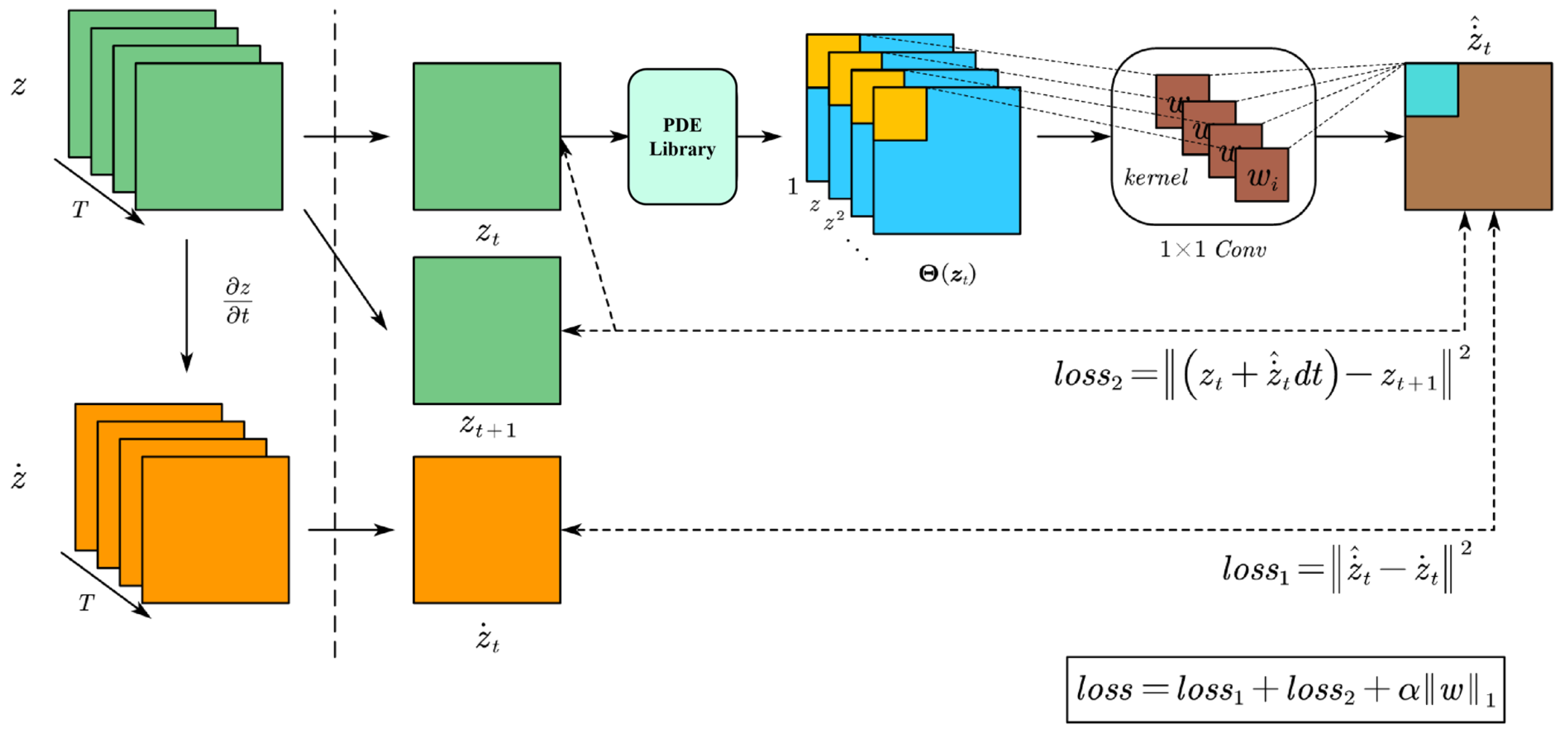
Based on these advantages, we propose a CNN-based method to solve the coefficients of the governing equations. This approach preserves the nonlinearity of the model while significantly improving solution accuracy. The architecture of the CNN and the solution process are illustrated in Figure 2, where the convolutional kernel size is set to $1\times 1$. Specifically, we approximate the derivative of the time series data z using the output of the CNN, denoted as ${\widehat{\dot{z}}}_t$. The loss function is then constructed based on the residuals as follows:

$$loss=\parallel (z_t+{\widehat{\dot{z}}}_t)d_t-z_{t+1}{\parallel }^2+\parallel ({\widehat{\dot{z}}}_t-{\dot{z}}_t){\parallel }^2+\alpha {\parallel w\parallel }_1,$$

(8)

where ${\alpha \parallel w\parallel }_1$ is a regularization term.

At the same time, sparsity is introduced through the application of the sequential threshold least squares method, which involves iteratively setting all coefficients less than the tolerance to 0. By choosing a specific tolerance and $\alpha$, this approach provides a sparse approximation for w.

2.3. Accuracy Evaluation

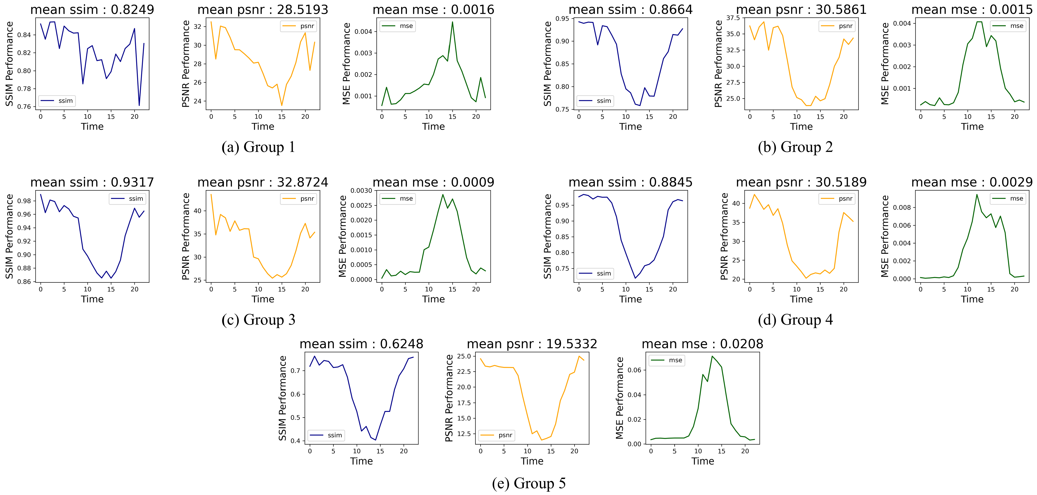
In order to accurately and objectively assess the model’s performance, this study utilizes three evaluation metrics from two distinct perspectives.

The first perspective involves time series regression evaluation metrics, specifically mean squared error (MSE), which is used to evaluate the temporal accuracy of the model’s predictions:

$$MSE={\displaystyle \frac{1}{m}}\sum _{i=1}^m{(y_i-\widehat{y_i})}^2,$$

In this equation, i represents the i-th sample point, $y_i$ denotes the NDVI value at the i-th time point for the time series of the given pixel, and $\widehat{y_i}$ and $\overline{y}$ represent the predicted and mean NDVI values, respectively. To eliminate the influence of spatial variations across different pixels, the MSE is computed for each pixel at different time points within the study area, and the average MSE across all pixels is used as the final evaluation metric. This procedure allows for a comprehensive assessment of the model’s temporal prediction accuracy.

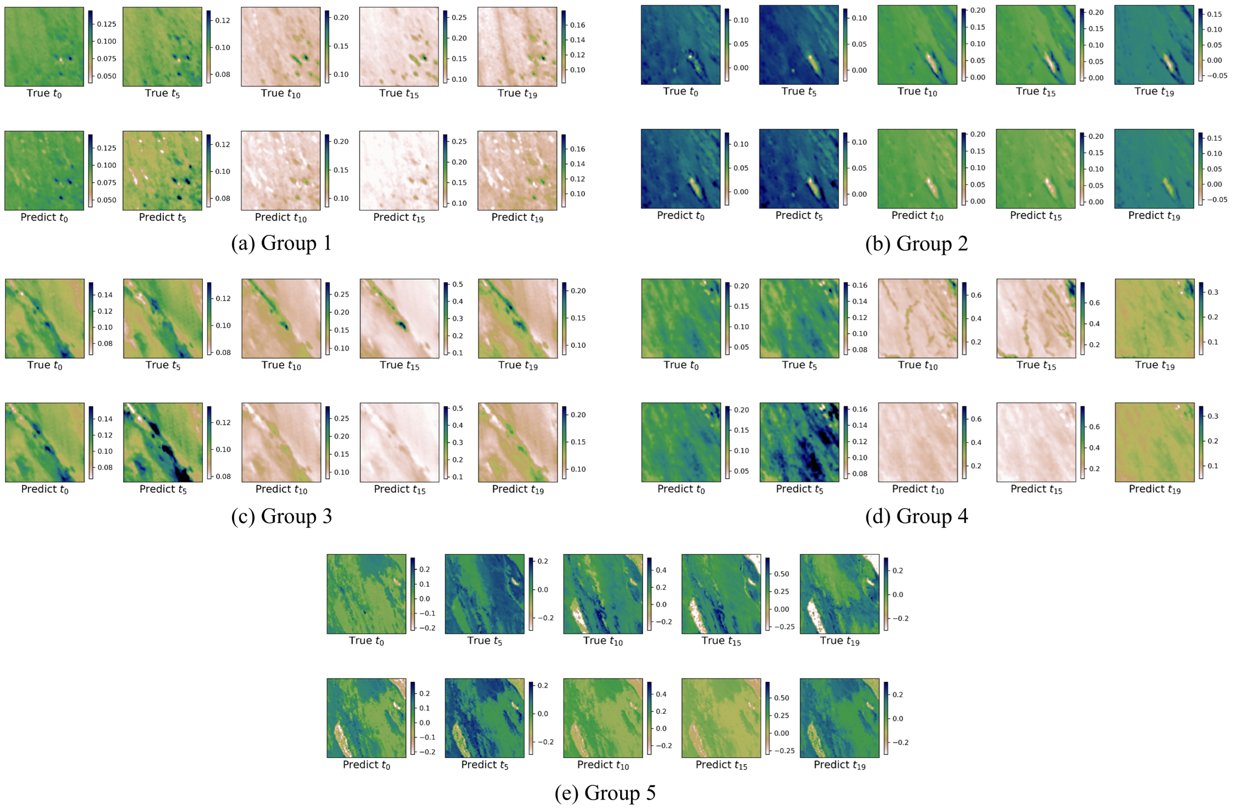
The second perspective concerns image quality assessment metrics, namely the structural similarity index (SSIM) and peak signal-to-noise ratio (PSNR). Unlike traditional pixel-by-pixel prediction, the model generates predictions for the entire image at each time point, making it crucial to compare the predicted image with the original image at the same time. The SSIM and PSNR metrics provide valuable measures for assessing image quality at each time point. The formulas for these metrics are as follows:

1. Structural similarity index (SSIM):

$$SSIM(x,y)={\displaystyle \frac{(2{\mu }_x{\mu }_y+c_1)(2{\sigma }_{xy}+c_2)}{({\mu }_x^2+{\mu }_y^2+c_1)({\sigma }_x^2+{\sigma }_y^2+c_2)}}$$

(9)

In this formula, ${\mu }_x$ and ${\mu }_y$ represent the mean values of images x and y, ${\sigma }_x^2$ and ${\sigma }_y^2$ are their variances, and ${\sigma }_{xy}$ is the covariance between x and y. Constants $c_1$ and $c_2$ are used to stabilize the calculation.

2. Peak signal-to-noise ratio (PSNR):

$$PSNR=10{log}_{10}\left({\displaystyle \frac{MA{X}_I^2}{MSE}}\right)$$

(10)

Here, $MA{X}_I$ is the maximum pixel value in the image and $MSE$ is the mean squared error.

The SSIM and PSNR metrics provide critical insight into the spatial accuracy of the model, comparing the structural and signal-to-noise relationships between the predicted and original images. These metrics are essential for evaluating how well the model preserves spatial features and image integrity during the prediction process.

3. Results

3.1. MODIS Data

3.1.1. Experimental Results

This part of the study is based on five $100\times 100$ MODIS image series that are randomly selected on orbit number H26V05. Among these areas, the proportion of the time series length of the training set to the test set is 9:1, which means that the data from 2001 to 2009 are used as the training set to predict the data from 2009 to 2010. We set $\alpha =1\times {10}^{-2}$ and the stochastic gradient descent (SGD) optimizer for optimizing the procedure, with an initial learning rate $lr=1\times {10}^{-2}$ for 3000 steps. The coefficients for Equation (5) are shown in

Table 1. The coefficients of governing equation for five groups of MODIS NDVI time series images. Coefficient values larger than the sparse threshold are shown in boldface.

Coefficient	Function	Group 1	Group 2	Group 3	Group 4	Group 5
$w_0$	1	$-1.6549\times {10}^{-10}$	$-3.4473\times {10}^{-10}$	$-2.9610\times {10}^{-6}$	$4.0603\times {10}^{-9}$	0.0039
$w_1$	z	$-4.8708\times {10}^{-11}$	$8.21888\times {10}^{-11}$	$-1.5214\times {10}^{-10}$	$3.8775\times {10}^{-11}$	$-4.4819\times {10}^{-5}$
$w_2$	$z^2$	$2.4429\times {10}^{-11}$	$-2.3844\times {10}^{-11}$	$-6.7377\times {10}^{-11}$	−0.0010	$-1.4637\times {10}^{-5}$
$w_3$	$sinz$	$-2.2910\times {10}^{-11}$	$1.3878\times {10}^{-11}$	$-1.2721\times {10}^{-10}$	$7.4993\times {10}^{-11}$	$-4.9363\times {10}^{-5}$
$w_4$	$cosz$	$-8.9835\times {10}^{-11}$	$-2.7204\times {10}^{-10}$	$-1.8378\times {10}^{-6}$	$3.9173\times {10}^{-9}$	0.0065
$w_5$	$z_y$	−0.0035	$9.2284\times {10}^{-11}$	$2.4362\times {10}^{-11}$	$9.0367\times {10}^{-12}$	$-1.1030\times {10}^{-6}$
$w_6$	$z_{yy}$	$3.7910\times {10}^{-11}$	$-2.1909\times {10}^{-11}$	$5.1522\times {10}^{-11}$	$1.6951\times {10}^{-11}$	$1.2401\times {10}^{-5}$
$w_7$	$z_x$	$1.7753\times {10}^{-11}$	$-9.1747\times {10}^{-11}$	$-1.9216\times {10}^{-12}$	$-8.3543\times {10}^{-12}$	$-1.9156\times {10}^{-6}$
$w_8$	$z_{xy}$	$-1.6184\times {10}^{-11}$	$-6.5886\times {10}^{-11}$	$3.8230\times {10}^{-11}$	$-3.9732\times {10}^{-12}$	$1.5522\times {10}^{-6}$
$w_9$	$z_{x}x$	$-2.5834\times {10}^{-11}$	$6.4549\times {10}^{-11}$	$8.0480\times {10}^{-11}$	$-4.8905\times {10}^{-13}$	$1.4457\times {10}^{-6}$
$w_{10}$	$z{z}_y$	$1.8727\times {10}^{-11}$	$-9.5009\times {10}^{-11}$	$-3.4025\times {10}^{-11}$	−0.0038	$-3.3938\times {10}^{-6}$
$w_{11}$	$z^2{z}_y$	$3.2440\times {10}^{-11}$	$-3.1690\times {10}^{-11}$	$9.6638\times {10}^{-11}$	$-7.8387\times {10}^{-12}$	$-1.1099\times {10}^{-6}$
$w_{12}$	$sinz{z}_y$	$1.1198\times {10}^{-11}$	$-6.4214\times {10}^{-11}$	$-3.6493\times {10}^{-11}$	$-1.6116\times {10}^{-12}$	$1.9176\times {10}^{-7}$
$w_{13}$	$cosz{z}_y$	$-4.0222\times {10}^{-11}$	$-1.1051\times {10}^{-11}$	−0.0159	$2.20208\times {10}^{-12}$	$-1.6926\times {10}^{-7}$
$w_{14}$	$z{z}_{yy}$	$-4.2453\times {10}^{-11}$	$4.7848\times {10}^{-11}$	$5.3971\times {10}^{-11}$	$3.0347\times {10}^{-12}$	0.0004
$w_{15}$	$z^2{z}_{yy}$	$-6.6411\times {10}^{-11}$	$4.6467\times {10}^{-11}$	$9.7276\times {10}^{-11}$	$6.6481\times {10}^{-12}$	$-4.1179\times {10}^{-6}$
$w_{16}$	$sinz{z}_{yy}$	$-1.4886\times {10}^{-11}$	$-1.3965\times {10}^{-11}$	$-6.6133\times {10}^{-11}$	$-1.4282\times {10}^{-12}$	0.0004
$w_{17}$	$cosz{z}_{yy}$	$1.6041\times {10}^{-11}$	$7.5267\times {10}^{-11}$	$3.4200\times {10}^{-11}$	$5.5996\times {10}^{-12}$	$5.7290\times {10}^{-6}$
$w_{18}$	$z{z}_x$	$9.3374\times {10}^{-13}$	$-7.7322\times {10}^{-11}$	$-3.2551\times {10}^{-11}$	$-1.9343\times {10}^{-12}$	$-4.4336\times {10}^{-7}$
$w_{19}$	$z^2{z}_x$	$5.6763\times {10}^{-11}$	$-3.0845\times {10}^{-11}$	$-6.5537\times {10}^{-12}$	$-6.2771\times {10}^{-13}$	$-7.7222\times {10}^{-7}$
$w_{20}$	$sinz{z}_x$	$9.8121\times {10}^{-11}$	$6.5410\times {10}^{-11}$	$9.5367\times {10}^{-11}$	−0.0104	$-1.4029\times {10}^{-7}$
$w_{21}$	$cosz{z}_x$	$4.3792\times {10}^{-11}$	$-2.6134\times {10}^{-11}$	$4.2308\times {10}^{-11}$	$-8.3419\times {10}^{-12}$	$-1.1577\times {10}^{-7}$
$w_{22}$	$z{z}_{xy}$	$1.0748\times {10}^{-11}$	$1.5929\times {10}^{-11}$	$-9.8331\times {10}^{-11}$	$1.9213\times {10}^{-12}$	$1.0074\times {10}^{-7}$
$w_{23}$	$z^2{z}_{xy}$	$-9.5430\times {10}^{-11}$	$-3.7896\times {10}^{-12}$	$7.0665\times {10}^{-11}$	0.0012	$-1.3203\times {10}^{-7}$
$w_{24}$	$sinz{z}_{xy}$	$6.3780\times {10}^{-11}$	$-2.2857\times {10}^{-11}$	$4.7830\times {10}^{-11}$	$-2.3408\times {10}^{-12}$	$-9.7212\times {10}^{-7}$
$w_{25}$	$cosz{z}_{xy}$	$9.7437\times {10}^{-11}$	$-4.6868\times {10}^{-11}$	$3.4963\times {10}^{-11}$	$1.8149\times {10}^{-12}$	$4.1621\times {10}^{-7}$
$w_{26}$	$z{z}_{xx}$	−0.0139	$3.1423\times {10}^{-11}$	$7.2105\times {10}^{-11}$	$4.8742\times {10}^{-12}$	$1.5332\times {10}^{-7}$
$w_{27}$	$z^2{z}_{xx}$	0.0088	−0.0078	$-9.1501\times {10}^{-11}$	$7.3123\times {10}^{-12}$	$-1.6999\times {10}^{-7}$
$w_{28}$	$sinz{z}_{xx}$	$7.7762\times {10}^{-11}$	$-5.4148\times {10}^{-11}$	$-8.6017\times {10}^{-12}$	$3.4911\times {10}^{-12}$	$4.7777\times {10}^{-7}$
$w_{29}$	$cosz{z}_{xx}$	$5.9721\times {10}^{-12}$	$5.7873\times {10}^{-11}$	$3.3040\times {10}^{-11}$	$1.2725\times {10}^{-11}$	$9.1855\times {10}^{-7}$

.

Based on these coefficients obtained by TS-PDE, the image prediction results are calculated from January to December of the year 2010. Figure 3 visually shows the prediction results of the five data groups, comparing original images and predicted images at different times, respectively. As can be seen from these images, the predicted images are similar to the original images with the naked eye. This implies that TS-PDE can accurately capture the trend of the original time series images and predict future images accordingly.

3.1.2. Sparse Results

Note that some values in the coefficient vector are very small, which significantly contributes to the sparsity that we aim to achieve. The sparsity is introduced by setting all coefficients to zero if they are less than ${10}^{-4}$. For each group of data, the corresponding coefficients of the sparse Equation (11) are presented in

Table 2. The sparse coefficients of governing equation for five groups of MODIS NDVI time series images.

Coefficient	Function	Group 1	Group 2	Group 3	Group 4	Group 5
$w_0$	1	0	0	0	0	0.0039
$w_1$	z	0	0	0	0	0
$w_2$	$z^2$	0	0	0	−0.0010	0
$w_3$	$sinz$	0	0	0	0	0
$w_4$	$cosz$	0	0	0	0	0.0065
$w_5$	$z_y$	−0.0035	0	0	0	0
$w_6$	$z_y$	0	0	0	0	0
$w_7$	$z_x$	0	0	0	0	0
$w_8$	$z_{xy}$	0	0	0	0	0
$w_9$	$z_{xx}$	0	0	0	0	0
$w_{10}$	$z{z}_y$	0	0	0	−0.0038	0
$w_{11}$	$z^2{z}_y$	0	0	0	0	0
$w_{12}$	$sinz{z}_y$	0	0	0	0	0
$w_{13}$	$cosz{z}_y$	0	0	−0.0159	0	0
$w_{14}$	$z{z}_{yy}$	0	0	0	0	0
$w_{15}$	$z^2{z}_{yy}$	0	0	0	0	0
$w_{16}$	$sinz{z}_{yy}$	0	0	0	0	0
$w_{17}$	$cosz{z}_{yy}$	0	0	0	0	0
$w_{18}$	$z{z}_x$	0	0	0	0	0
$w_{19}$	$z^2{z}_x$	0	0	0	0	0
$w_{20}$	$sinz{z}_x$	0	0	0	−0.0104	0
$w_{21}$	$cosz{z}_x$	0	0	0	0	0
$w_{22}$	$z{z}_{xy}$	0	0	0	0	0
$w_{23}$	$z^2{z}_{xy}$	0	0	0	0.0012	0
$w_{24}$	$sinz{z}_{xy}$	0	0	0	0	0
$w_{25}$	$cosz{z}_{xy}$	0	0	0	0	0
$w_{26}$	$z{z}_{xx}$	−0.0139	0	0	0	0
$w_{27}$	$z^2{z}_{xx}$	0.0088	−0.0078	0	0	0
$w_{28}$	$sinz{z}_{xx}$	0	0	0	0	0
$w_{29}$	$cosz{z}_{xx}$	0	0	0	0	0

. A synthesis of the findings from the five data groups reveals that 10 equation terms are involved, including the constant term, the squared term, the sine and cosine terms, and their combinations. Given a sparse constraint, the governing equation of MODIS NDVI time series in this study can be expressed in the following form:

$$\begin{array}{cc}\hfill z[t+1]-z\left[t\right]=& w_0+w_2{z}^2\left[t\right]+w_{4}cosz\left[t\right]\hfill \\ \hfill & +(w_5+w_{10}z\left[t\right]+w_{13}cosz\left[t\right])z_y\left[t\right]\hfill \\ \hfill & +w_{20}sinz\left[t\right]z_x\left[t\right]+w_{23}{z}^2\left[t\right]z_{xy}\left[t\right]\hfill \\ \hfill & +(w_{26}z\left[t\right]+w_{27}{z}^2\left[t\right])z_{xx}\left[t\right],\hfill \end{array}$$

(11)

To quantify the prediction accuracy of the discovered equation, three indicators, PSNR, SSIM, and MSE, regarding the image quality are evaluated and shown in Figure 4 and

Table 3. Mean results for quantitative evaluation indicators on five groups of MODIS NDVI data.

Mean	Group 1	Group 2	Group 3	Group 4	Group 5
SSIM↑	0.8249	0.8664	0.9317	0.8845	0.6248
PSNR↑	28.5193	30.5861	32.8724	30.5189	19.5332
MSE↓	0.0016	0.0015	0.0009	0.0029	0.0208

. These time series values in Figure 4 are obtained by picking points at certain intervals, and Table 3 summarizes the average of each group. The results presented in Figure 4 and Table 3 indicate that the initial four groups of data exhibited superior performance, with mean SSIM values exceeding 0.82, mean PSNR values ranging from 28.5 to 32.8, and mean MSE values approximating $9\times {10}^{-4}$. In contrast, the fifth group demonstrated comparatively lower predictive performance than the first four groups.

3.2. Planet Data

3.2.1. Experimental Results

The Planet dataset is complementary to the MODIS dataset in terms of both temporal and spatial resolution. Concretely, the time interval of Planet images is one day and the spatial resolution is 3 m. NDVI values are calculated from the Planet image time series located at Brandenburg, Germany in 2018. To make the experimental settings consistent with the MODIS dataset, we also choose five groups of data randomly. Each group of data is divided into a training part and testing part using the same proportion of time series length as in the previous MODIS dataset, which means that the first 329 days are used for training and we will predict the images of the last 36 days for every group of data. In addition to this, let $\alpha =8\times {10}^{-3}$, and we use the SGD optimizer with learning rate $lr=1\times {10}^{-3}$ and step number 3000. The discovered coefficients for each group of data are shown in

Table 4. The coefficients of governing equation for five groups of Planet NDVI time series images. Coefficient values larger than the sparse threshold are shown in boldface.

Coefficient	Function	Group 1	Group 2	Group 3	Group 4	Group 5
$w_0$	1	0.0030	−0.0012	−0.0043	0.0075	0.0038
$w_1$	z	−0.0001	−0.0169	$3.3518\times {10}^{-5}$	$-1.1156\times {10}^{-5}$	$-5.6450\times {10}^{-6}$
$w_2$	$z^2$	$2.6886\times {10}^{-6}$	$-6.2799\times {10}^{-6}$	$9.3197\times {10}^{-6}$	$-1.1868\times {10}^{-5}$	$-3.6212\times {10}^{-6}$
$w_3$	$sinz$	$-5.3116\times {10}^{-6}$	$-1.6602\times {10}^{-6}$	$2.6055\times {10}^{-5}$	0.0002	$-1.0531\times {10}^{-5}$
$w_4$	$cosz$	$2.1110\times {10}^{-6}$	$1.8319\times {10}^{-5}$	−0.0167	0.0023	0.0003
$w_5$	$z_y$	$2.4512\times {10}^{-6}$	$6.5409\times {10}^{-6}$	$8.6950\times {10}^{-6}$	$-3.5497\times {10}^{-6}$	$-4.8108\times {10}^{-6}$
$w_6$	$z_{yy}$	$-8.0430\times {10}^{-6}$	$4.4267\times {10}^{-6}$	$-6.5704\times {10}^{-6}$	$-5.6216\times {10}^{-7}$	$5.0810\times {10}^{-6}$
$w_7$	$z_x$	$2.3690\times {10}^{-6}$	$-4.5934\times {10}^{-6}$	$-4.9591\times {10}^{-6}$	$-4.1198\times {10}^{-6}$	$5.7990\times {10}^{-6}$
$w_8$	$z_{xy}$	$6.8517\times {10}^{-6}$	$-2.9670\times {10}^{-6}$	$-6.3390\times {10}^{-6}$	$1.4971\times {10}^{-6}$	$-1.6837\times {10}^{-6}$
$w_9$	$z_{xx}$	$-2.0397\times {10}^{-6}$	$-3.2049\times {10}^{-6}$	$-6.4667\times {10}^{-6}$	$6.6738\times {10}^{-6}$	$3.6177\times {10}^{-6}$
$w_{10}$	$z{z}_y$	$-5.1383\times {10}^{-6}$	$6.1656\times {10}^{-6}$	$-4.7921\times {10}^{-6}$	$-2.0825\times {10}^{-6}$	$8.8088\times {10}^{-7}$
$w_{11}$	$z^2{z}_y$	$5.8518\times {10}^{-8}$	$-4.3677\times {10}^{-6}$	$-7.4058\times {10}^{-6}$	$2.9550\times {10}^{-6}$	$3.0995\times {10}^{-6}$
$w_{12}$	$sinz{z}_y$	$3.0900\times {10}^{-6}$	$-2.2845\times {10}^{-6}$	$-6.3577\times {10}^{-6}$	$1.0314\times {10}^{-6}$	$-5.7671\times {10}^{-6}$
$w_{13}$	$cosz{z}_y$	$-4.2573\times {10}^{-6}$	$6.7408\times {10}^{-6}$	$-4.9776\times {10}^{-6}$	$-7.2742\times {10}^{-6}$	$-3.4729\times {10}^{-6}$
$w_{14}$	$z{z}_{yy}$	$-4.4218\times {10}^{-6}$	$2.8561\times {10}^{-7}$	$-1.7717\times {10}^{-6}$	$-7.2811\times {10}^{-6}$	$-3.0958\times {10}^{-6}$
$w_{15}$	$z^2{z}_{yy}$	$1.1360\times {10}^{-6}$	$1.4643\times {10}^{-7}$	$-3.1533\times {10}^{-6}$	$3.1422\times {10}^{-6}$	$6.2442\times {10}^{-6}$
$w_{16}$	$sinz{z}_{yy}$	$-2.1022\times {10}^{-6}$	$-1.1169\times {10}^{-6}$	$2.9475\times {10}^{-6}$	$2.2768\times {10}^{-6}$	$4.1985\times {10}^{-6}$
$w_{17}$	$cosz{z}_{yy}$	$1.5388\times {10}^{-6}$	$6.8322\times {10}^{-6}$	$3.6638\times {10}^{-6}$	$6.1930\times {10}^{-6}$	$6.7549\times {10}^{-6}$
$w_{18}$	$z{z}_x$	$-3.7480\times {10}^{-6}$	$7.7792\times {10}^{-7}$	$-4.7479\times {10}^{-6}$	$5.5431\times {10}^{-6}$	$-7.7971\times {10}^{-6}$
$w_{19}$	$z^2{z}_x$	$5.6013\times {10}^{-7}$	$-2.6345\times {10}^{-7}$	$3.3629\times {10}^{-6}$	$-2.4354\times {10}^{-6}$	$-6.8442\times {10}^{-6}$
$w_{20}$	$sinz{z}_x$	$-2.1065\times {10}^{-6}$	$-3.836\times {10}^{-6}$	$-6.5694\times {10}^{-6}$	$4.8093\times {10}^{-6}$	$3.7605\times {10}^{-7}$
$w_{21}$	$cosz{z}_x$	$3.8484\times {10}^{-6}$	$-4.9716\times {10}^{-6}$	$4.7602\times {10}^{-6}$	$-5.0270\times {10}^{-6}$	$1.9650\times {10}^{-6}$
$w_{22}$	$z{z}_{xy}$	$-5.6550\times {10}^{-6}$	$-1.0133\times {10}^{-6}$	$-7.1469\times {10}^{-6}$	$3.6105\times {10}^{-6}$	$-5.7685\times {10}^{-6}$
$w_{23}$	$z^2{z}_{xy}$	$-9.4088\times {10}^{-7}$	$-2.3748\times {10}^{-6}$	$2.9650\times {10}^{-6}$	$-7.7972\times {10}^{-6}$	$3.1755\times {10}^{-6}$
$w_{24}$	$sinz{z}_{xy}$	$4.8035\times {10}^{-6}$	$4.6814\times {10}^{-7}$	$5.7442\times {10}^{-6}$	$5.6675\times {10}^{-7}$	$-4.3752\times {10}^{-6}$
$w_{25}$	$cosz{z}_{xy}$	$7.1195\times {10}^{-6}$	$1.0732\times {10}^{-6}$	$-1.4570\times {10}^{-6}$	$-2.8132\times {10}^{-6}$	$6.8784\times {10}^{-6}$
$w_{26}$	$z{z}_{xx}$	$1.2967\times {10}^{-7}$	$-2.1219\times {10}^{-6}$	$1.4992\times {10}^{-6}$	$-5.9203\times {10}^{-6}$	$-3.2486\times {10}^{-6}$
$w_{27}$	$z^2{z}_{xx}$	$3.7339\times {10}^{-7}$	$8.0346\times {10}^{-6}$	$-3.9942\times {10}^{-6}$	$-1.5101\times {10}^{-6}$	$3.92488\times {10}^{-6}$
$w_{28}$	$sinz{z}_{xx}$	$5.4570\times {10}^{-6}$	$1.0093\times {10}^{-5}$	$-6.0852\times {10}^{-6}$	$-3.5602\times {10}^{-6}$	$-5.8069\times {10}^{-6}$
$w_{29}$	$cosz{z}_{xx}$	$7.3424\times {10}^{-6}$	$2.3690\times {10}^{-6}$	$1.6302\times {10}^{-6}$	$5.6630\times {10}^{-6}$	$6.8527\times {10}^{-6}$

.

According to these coefficients, the corresponding NDVI values can be predicted to generate the comparison images for the upcoming 36-day period, as shown in Figure 5. In each set of images, the upper side represents the predicted image and the bottom side represents the original image. It can be seen from these figures that the difference between each group of images is small.

3.2.2. Sparse Results

For the Planet dataset, we set the tolerance of sparsity as ${10}^{-5}$, and the sparse version of the dominant equation is given as follows:

$$z[t+1]-z\left[t\right]=w_0+w_{1}z\left[t\right]+w_{3}sinz\left[t\right]+w_{4}cosz\left[t\right],$$

(12)

where the sparse coefficients for each group are presented in the following

Table 5. The sparse coefficients of governing equation for five groups of Planet NDVI time series images.

Coefficient	Function	Group 1	Group 2	Group 3	Group 4	Group 5
$w_0$	1	0.0030	−0.0012	−0.0043	0.0075	0.0038
$w_1$	z	−0.0001	−0.0169	0	0	0
$w_2$	$z^2$	0	0	0	0	0
$w_3$	$sinz$	0	0	0	0.0002	0
$w_4$	$cosz$	0	0	−0.0167	0.0023	0.0003
$w_5$	$z_y$	0	0	0	0	0
$w_6$	$z_{yy}$	0	0	0	0	0
⋮	⋮	⋮	⋮	⋮	⋮	⋮
$w_{27}$	$z^2{z}_{xx}$	0	0	0	0	0
$w_{28}$	$sinz{z}_{xx}$	0	0	0	0	0
$w_{29}$	$cosz{z}_{xx}$	0	0	0	0	0

:

Figure 6 highlights the superior performance of TS-PDE in PSNR, SSIM, and MSE metrics, with average SSIM values exceeding 0.81 across all datasets. Notably, the fifth dataset demonstrates an average SSIM greater than 0.95, an average PSNR exceeding 30, and an average MSE of 0.0010 as shown in

Table 6. Mean results for quantitative evaluation indicators on five groups of Planet NDVI data.

Mean	Group 1	Group 2	Group 3	Group 4	Group 5
SSIM↑	0.9588	0.8125	0.8737	0.8996	0.9538
PSNR↑	29.4778	24.6567	26.6997	25.1333	30.9084
MSE↓	0.0014	0.0038	0.0042	0.0039	0.0010

. These results indicate that the structural information of the predicted images closely aligns with the original images, reflecting a high quality in prediction accuracy. An analysis of the five datasets presented in the figure reveals that SSIM and PSNR values decrease as the prediction time span increases, while MSE values exhibit an upward trend. As illustrated in Figure 6, the prediction accuracy of the TS-PDE method tends to degrade over longer time horizons. This phenomenon can be attributed to several factors:

• Accumulation of Errors: Over time, small errors in the predicted land cover dynamics can accumulate, leading to larger deviations from the actual values. This is particularly evident in complex systems where nonlinear interactions amplify uncertainties.
• Temporal Variability: The value of the NDVI is influenced by a wide range of time-dependent factors, such as seasonal changes, climate variability, and human activities. While the TS-PDE method captures these factors to some extent, their long-term behavior can be difficult to predict with high precision.
• Limitations of Training Data: The model is trained on historical data, which may not fully capture future trends or unprecedented events (e.g., extreme weather or rapid urbanization). As a result, predictions over longer time horizons are inherently more uncertain.

4. Discussion

4.1. Physical Significance

In this study, convolutional neural networks (CNNs) combined with sparse regression methods are utilized to analyze datasets at varying spatial resolutions, enabling the extraction of governing equations that describe the underlying dynamics. For low-resolution MODIS images, as shown in

Table 7. The discovered equations for five groups of MODIS NDVI data.

Data Group	Discovered Equation	Discovered Term Count
Group 1	$z[t+1]-z\left[t\right]=-0.0035z_y\left[t\right]+(-0.0139z\left[t\right]+0.0088z^2\left[t\right])z_{xx}\left[t\right]$	3
Group 2	$z[t+1]-z\left[t\right]=-0.0078z^2\left[t\right]z_{xx}\left[t\right]$	3
Group 3	$z[t+1]-z\left[t\right]=-0.0159cosz\left[t\right]z_y\left[t\right]$	4
Group 4	$z[t+1]-z\left[t\right]=-0.0010z^2\left[t\right]-0.0038z\left[t\right]z_y\left[t\right]-0.0104sinz\left[t\right]z_x\left[t\right]+0.0012z^2\left[t\right]z_{xy}\left[t\right]$	8
Group 5	$z[t+1]-z\left[t\right]=0.0039+0.0065cosz\left[t\right]$	10
Integration	$z[t+1]-z\left[t\right]=w_0+w_2{z}^2\left[t\right]+w_{4}cosz\left[t\right]+(w_5+w_{10}z\left[t\right]+w_{13}cosz\left[t\right])z_y\left[t\right]$	10
	$+w_{20}sinz\left[t\right]z_x\left[t\right]+w_{23}{z}^2\left[t\right]z_{xy}\left[t\right]+(w_{26}z\left[t\right]+w_{27}{z}^2\left[t\right])z_{xx}\left[t\right]$

, the extracted equations comprise ten different terms, indicating a relatively higher level of complexity, likely due to the coarser spatial resolution and additional variability in the data (e.g., cloud and shadow pixels).

In contrast, as shown in

Table 8. The discovered equations for five groups of Planet NDVI data.

Data Group	Discovered Equation	Discovered Term Count
Group 1	$z[t+1]-z\left[t\right]=0.0030-0.0001z\left[t\right]$	2
Group 2	$z[t+1]-z\left[t\right]=-0.0012-0.0169z\left[t\right]$	2
Group 3	$z[t+1]-z\left[t\right]=-0.0043-0.0167cosz\left[t\right]$	3
Group 4	$z[t+1]-z\left[t\right]=0.0075+0.0002sinz\left[t\right]+0.0023cosz\left[t\right]$	4
Group 5	$z[t+1]-z\left[t\right]=0.0038+0.0003cosz\left[t\right]$	4
Integration	$z[t+1]-z\left[t\right]=w_0+w_{1}z\left[t\right]+w_{3}sinz\left[t\right]+w_{4}cosz\left[t\right]$	4

, the equations derived from high-resolution Planet images are significantly more concise, consisting of four different terms in total. This simplicity suggests that high-resolution data inherently capture dominant patterns more effectively, minimizing the need for complex mathematical descriptions. Furthermore, if the left-hand side of the equation is interpreted as the first derivative of the NDVI value with respect to time, it can be inferred that the NDVI values of high-resolution Planet images follow a sinusoidal relationship over time. This periodic behavior reflects the regular, cyclic nature of the underlying environmental or vegetation dynamics, such as seasonal growth and decay patterns, which are more precisely captured in high-resolution imagery.

However, the physical significance of these equations requires further exploration and discussion. Understanding the broader implications and connections between the mathematical representations and the underlying physical processes will provide deeper insights into the dynamics of vegetation and environmental systems represented by the extracted equations. For instance, the first-order derivative terms of x or y coordinates may indicate the influence of longitude or latitude on land cover, while the hybrid derivatives of x and y, or their second-order derivative terms, still need more interpretation.

4.2. Limitations

The current approach faces significant challenges in terms of physical interpretability, particularly when applied to low-resolution MODIS data. As Table 8 shows, the dominant equation of Planet data contains five terms, that is, constant terms, first-order terms, and trigonometric terms. This means that the value of the NDVI approximately exhibits a trigonometric relationship with time. But, unlike high-resolution Planet data, where the dominant equation offers a clear and concise representation of the underlying dynamics, the dominant equation derived from MODIS data is more complex and less intuitive. The complexity of the function is characterized by 10 terms as shown in Table 7, including the squared term, the trigonometric term, and the derivative terms for x and y. It is acknowledged that the derivative terms frequently possess a physical meaning associated with the rate of change. Consequently, the first-order derivative term for x can be conceptualized as the rate of change in the NDVI value along the latitude axis, while the first-order derivative term for y can be interpreted as the rate of change in the NDVI value along the longitude axis. In addition to this, the dominant equation contains a combination of trigonometric and derivative terms, which we conjecture is since the NDVI values demonstrate a trigonometric trend in time and are influenced by the surrounding environment (i.e., the dominant equation contains terms related to the rate of change in latitude and longitude). However, due to the complexity of the terms, it is difficult for us to obtain a direct physical explanation. Furthermore, the dominant equations vary considerably across the five datasets, with non-zero terms differing significantly between them. This inconsistency adds another layer of difficulty in uncovering a consistent physical meaning from the low-resolution data equations. To address these limitations, future work could explore tailored methods for low- and high-resolution data, such as simplifying equation structures for low-resolution data or leveraging multi-scale modeling techniques to enhance interpretability while maintaining accuracy.

Another limitation lies in the manual construction of the candidate function set used in this study. This restricts the derived equation terms to those predefined in the candidate set, making it impossible to identify more complex or unconventional equation forms. If the true dominant equation involves terms beyond the scope of the manually defined candidate set, the approach will fail to capture these dynamics accurately, leading to incomplete or erroneous results. This limitation highlights the need for automated or adaptive methods to expand the range of candidate functions and improve the robustness of the derived equations.

4.3. Future Work

Future research will endeavor to address several key limitations identified in this study and further improve the effectiveness and applicability of the methodology. Firstly, to improve the physical interpretability of the derived equations, we will explore ways to extract the underlying dynamics more efficiently from low-resolution MODIS data. This includes the development of more advanced techniques to deal with the complexity and variability of the key equations, thereby facilitating the identification of meaningful physical relationships between different datasets. Specifically, future work could improve the sophistication of the technique in terms of the set of candidate functions to explore the underlying equation forms more flexibly and comprehensively by adopting an adaptive approach to ensure that the derived equations more accurately reflect the true dynamics of the system.

Secondly, in order to validate the effectiveness of the method, future work could include evaluating the TS-PDE method using a wider range of remote sensing parameters to assess its accuracy and versatility, such as the enhanced vegetation index (EVI) and the soil-adjusted vegetation index (SAVI), which could be utilized to complement the NDVI, thereby capturing additional aspects of vegetation health and structure. Spectral band data could be employed to assess the capacity of models to capture finer spectral detail and enhance prediction accuracy using multispectral or hyperspectral data.

Moreover, to evaluate the generalizability of the TS-PDE method, its application will be extended to areas exhibiting diverse environmental characteristics, including arid zones, tropical forests, and urban areas. This approach will facilitate the acquisition of knowledge regarding the adaptability and generalizability of the method within varied ecological systems.

Historically, NDVI prediction has predominantly relied on time series analysis methods, including classical statistical approaches like the autoregressive integrated moving average (ARIMA) [24], deep learning architectures such as LSTM [33], and hybrid models combining convolutional and temporal networks like TSD-CNN-LSTM [30] and SF-CNN [31]. Recent advancements have further enhanced spatial–temporal modeling through integrated frameworks like ConvLSTM-SAC-NL [32], which couples a CNN with attention mechanisms for improved spatial dependency capture. However, a critical limitation persists: none of these methods provide explicit mathematical equations to describe the NDVI’s intrinsic dynamics. The TS-PDE framework addresses this gap by deriving interpretable partial differential equations that explicitly characterize NDVI evolution. This represents a significant advancement over purely data-driven approaches, offering both predictive capability and mechanistic insights. Despite this progress, TS-PDE currently relies on manually constructed candidate functions for equation discovery, which inherently constrains its flexibility and generalizability. To overcome this limitation, future work will integrate symbolic genetic algorithms [13]—a class of deep learning-driven evolutionary methods that enable the automated discovery of free-form equations without predefined templates. The integration of deep learning techniques [12,17,18,34] holds particular promise for advancing NDVI modeling. These methods excel at handling complex nonlinear systems and high-dimensional interactions, potentially enhancing both prediction accuracy and temporal extrapolation capabilities. Our ongoing research focuses on replacing traditional sparse-regression-based equation solvers with deep learning architectures, aiming to develop a unified framework that combines the interpretability of PDE-based modeling with the adaptive power of neural networks. This hybrid approach seeks to transcend the limitations of current methodologies, ultimately enabling a more robust and generalizable modeling of land cover dynamics while preserving physical interpretability.

5. Conclusions

This study introduces a novel approach for dynamic land cover modeling, termed TS-PDE. The TS-PDE method integrates spatiotemporal information by utilizing a combination of convolutional neural networks and sparse regression algorithms to uncover the dynamic equations governing land cover changes from satellite images. The accuracy of the TS-PDE prediction method is evaluated using NDVI time series data, assessing both temporal and spatial prediction capabilities.

The main findings of this study are as follows:

• The proposed TS-PDE method effectively overcomes the limitations of short-term and single-pixel prediction in existing land cover time series prediction methods by discovering a global spatiotemporal governing equation.
• For low-resolution data (MODIS data), the TS-PDE method generates a governing equation comprising diverse functional terms, offering a more comprehensive representation of land cover dynamics.
• For high-resolution data (Planet data), the TS-PDE method produces a more concise and consistent governing equation, consisting of only a constant term and one or two simple terms. This may indicate that spatiotemporal details are more sufficiently exhibited and captured with high spatial and temporal resolution images, while, for low-resolution or unprocessed images, information is mixed in pixels such that unified equations are hard to present.

Furthermore, the derived dominant equations are capable of making long-term predictions, with the differences between predicted results and actual observations remaining minimal, thereby ensuring high prediction accuracy.

In the future, the TS-PDE method is expected to have considerable potential in supporting governments and environmental agencies in land cover monitoring and management. Specifically, it can be applied to assess agricultural land use by enabling policymakers to optimize crop yields, identify areas at risk of degradation, and support precision farming initiatives. Furthermore, the method is poised to play a significant role in climate change mitigation by offering insights into the long-term dynamics of carbon sinks, such as forests and wetlands. This, in turn, will inform strategies for both mitigation and adaptation. To realize these applications, future work will focus on enhancing the scalability and accessibility of the TS-PDE method. This will include the development of user-friendly software tools and the integration of the framework with existing geospatial platforms. The TS-PDE framework is a transformative approach to understanding and managing land cover dynamics that bridges the gap between data-driven learning and physical modeling. Its applications have far-reaching implications for environmental sustainability and policy making, paving the way for more informed and effective decision making in the face of global environmental challenges.