
Multi-Decadal Shoreline Variability Along the Cap Ferret Sand Spit (SW France) Derived from Satellite Images


Abstract
1. Introduction
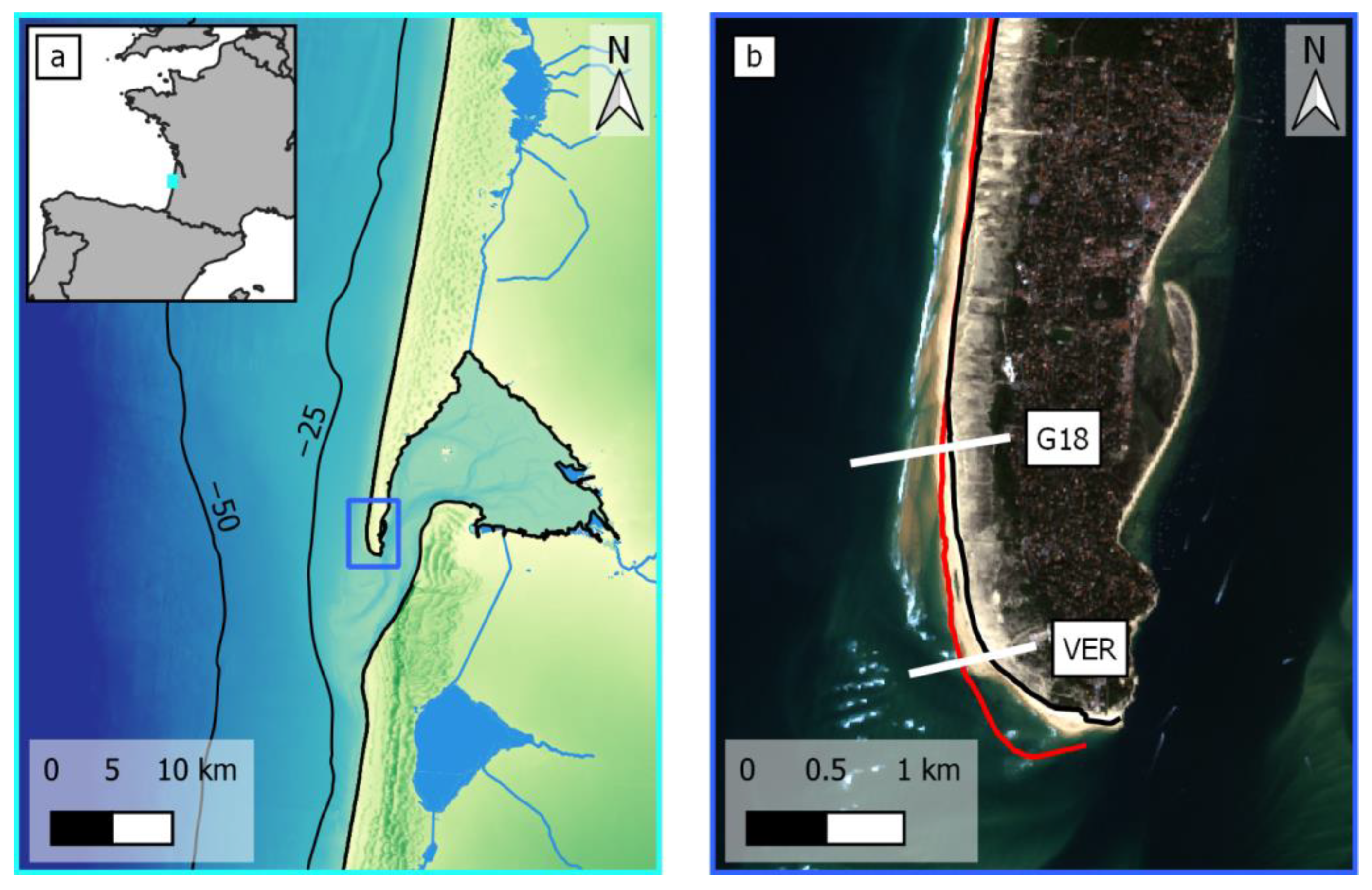
2. Study Site
3. Materials and Methods
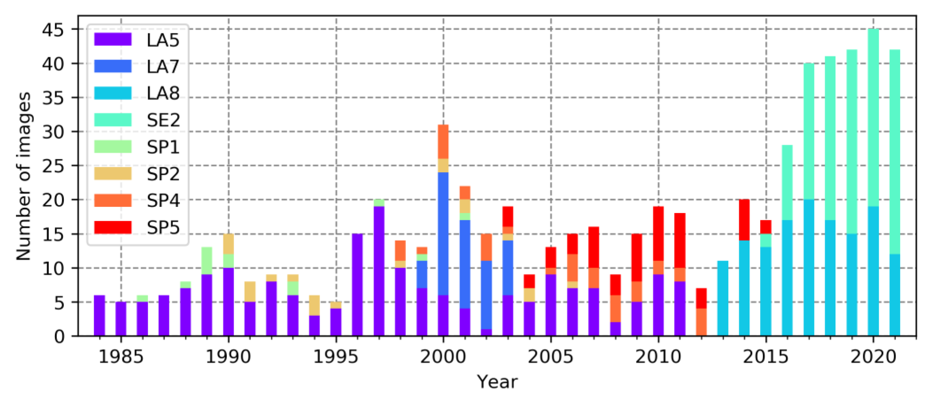
3.1. Satellite Images
3.2. Topographic Surveys and Shorelines
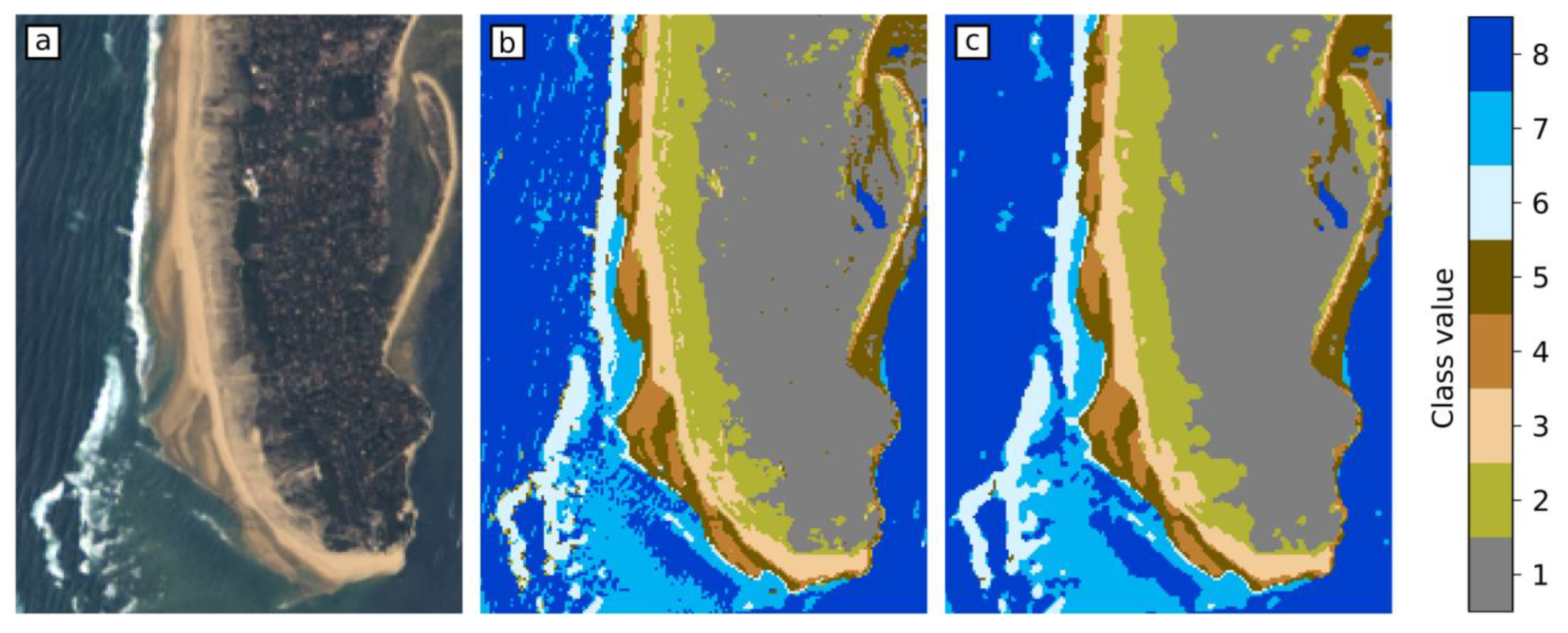
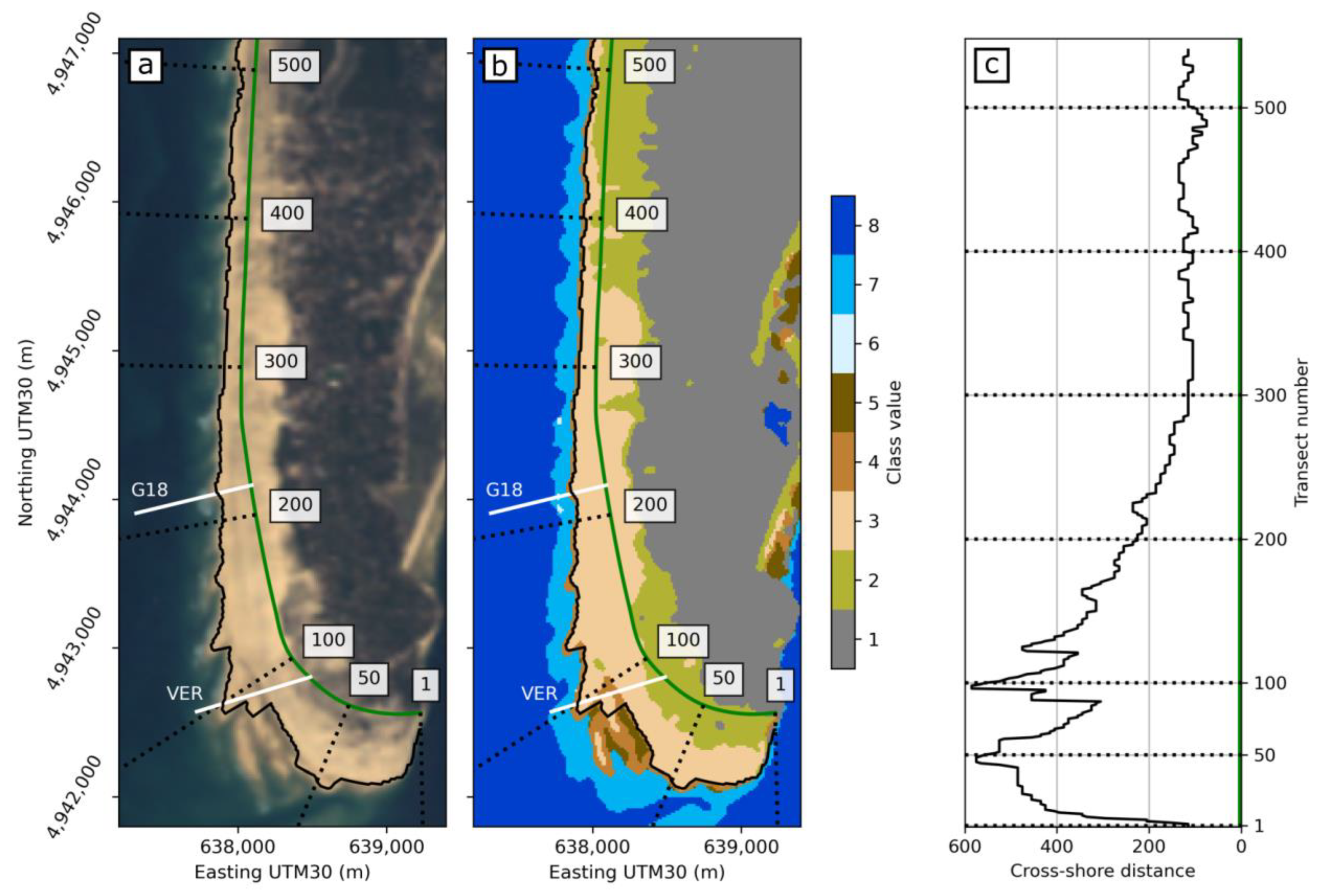
3.3. Supervised Classification
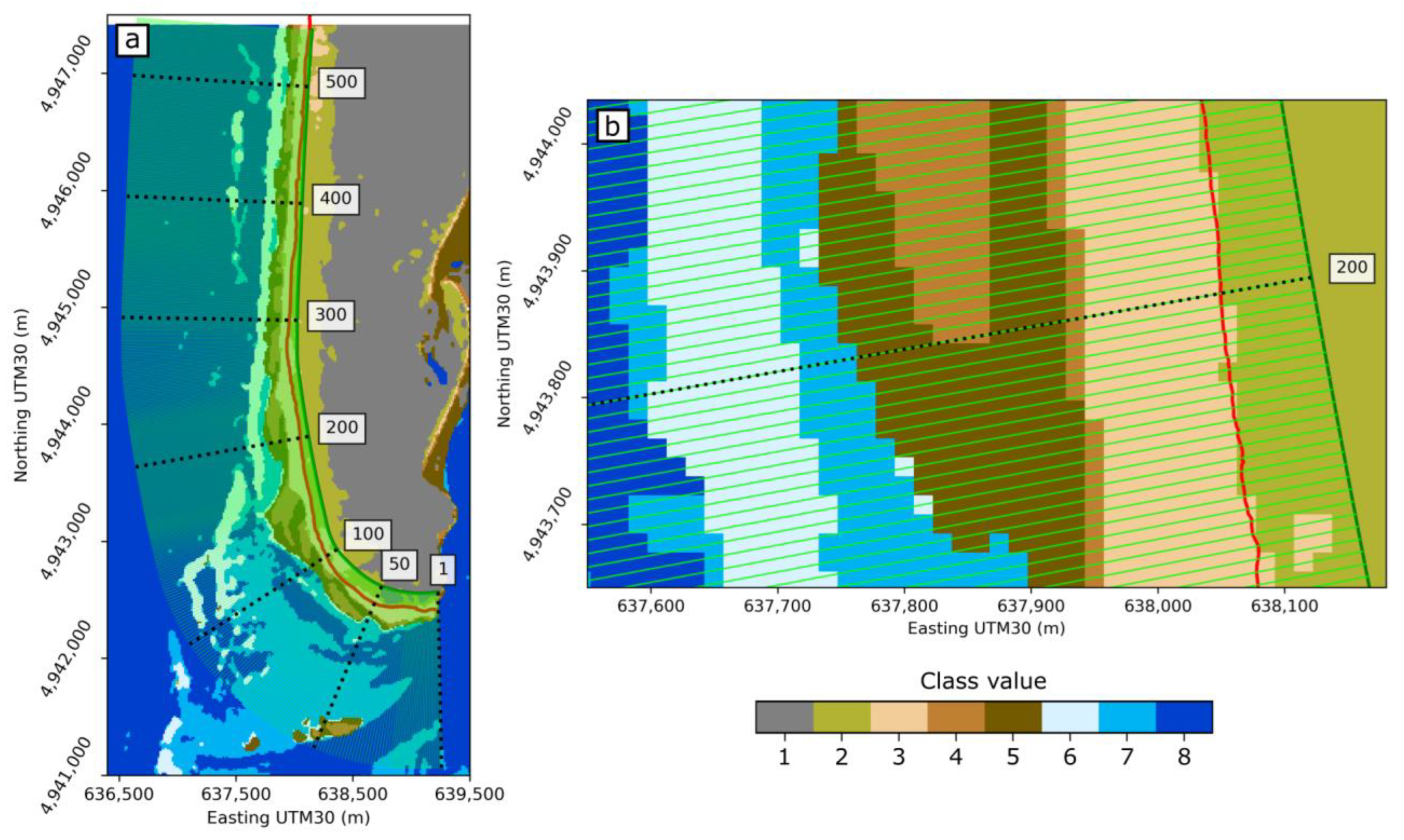
3.4. Wet/Dry Line Detection
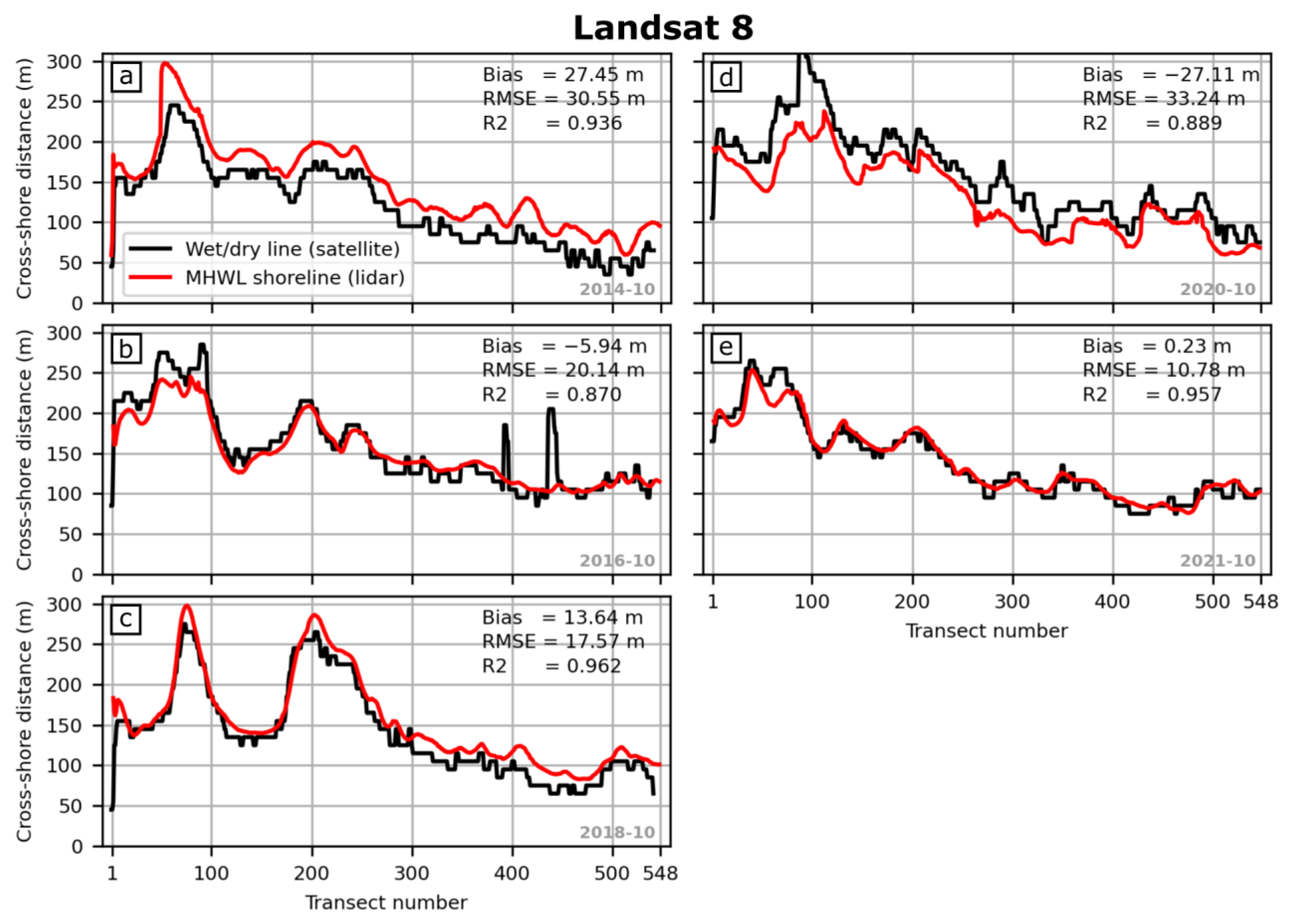
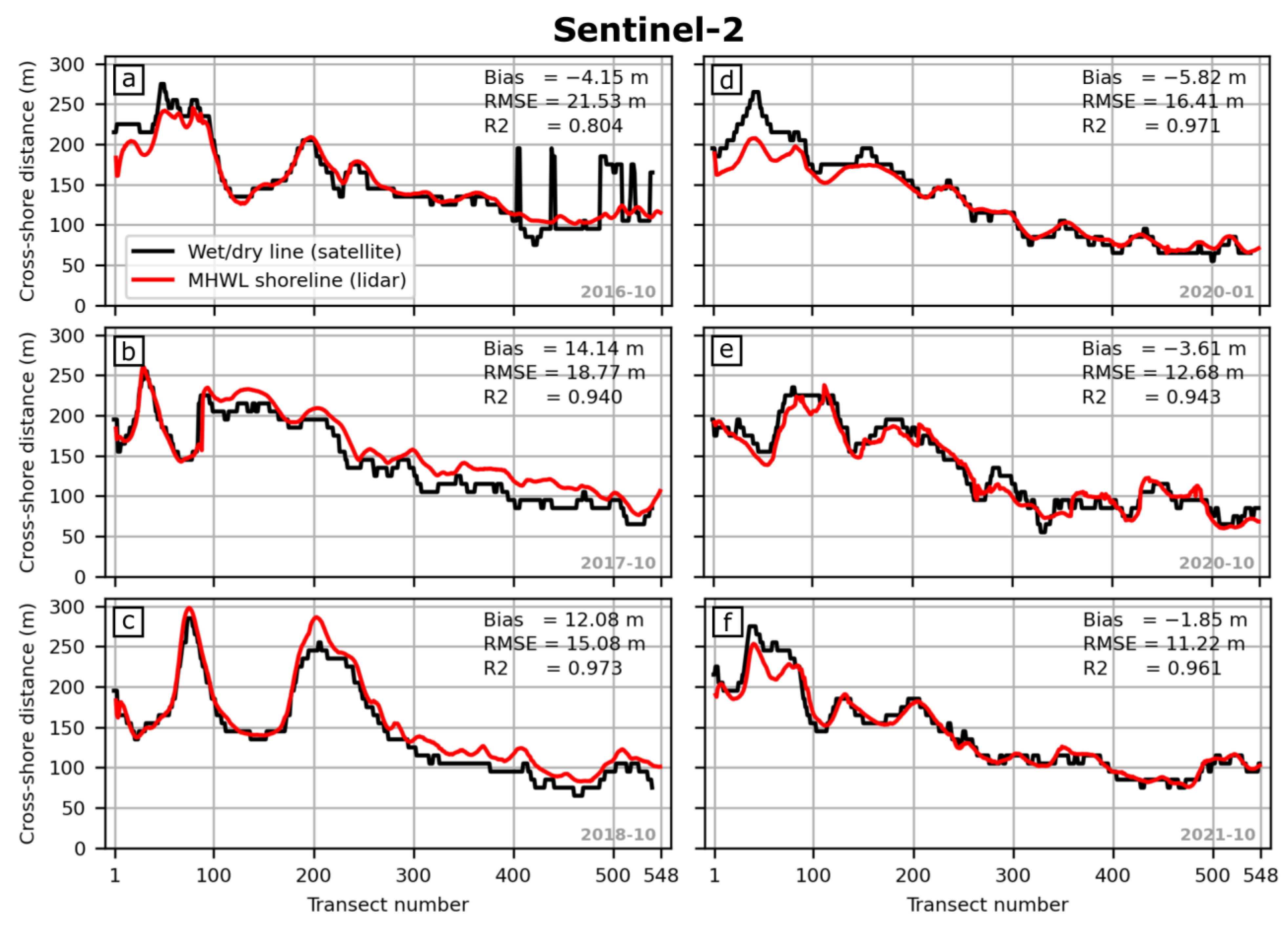
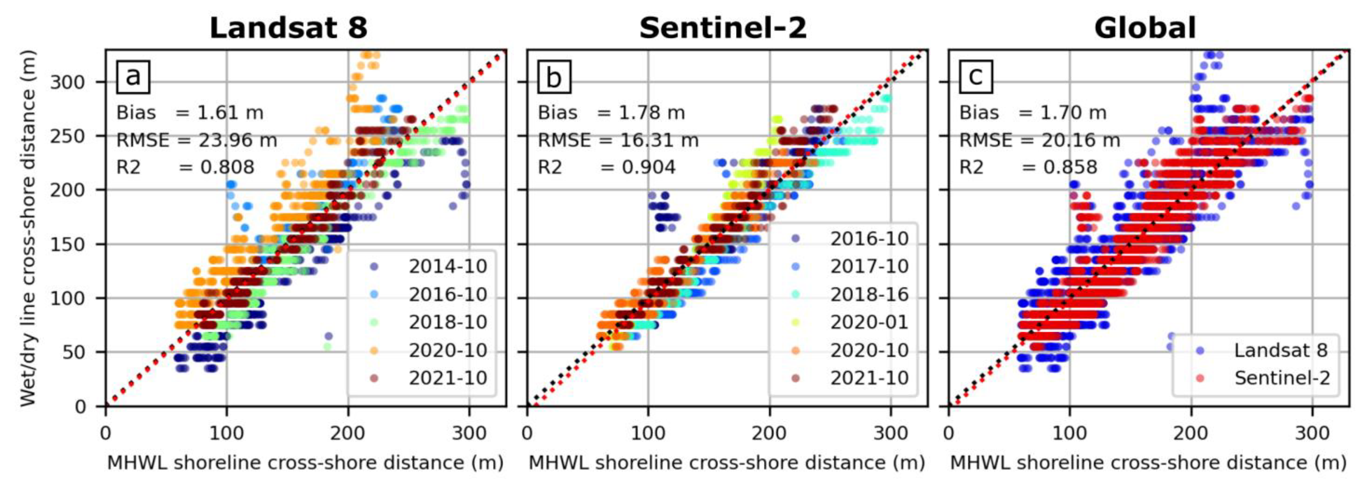
3.5. Comparison with Measurements
3.6. Wet/Dry Line Post-Processing
4. Results
4.1. Relation Between Wet/Dry Line and MHW Shoreline
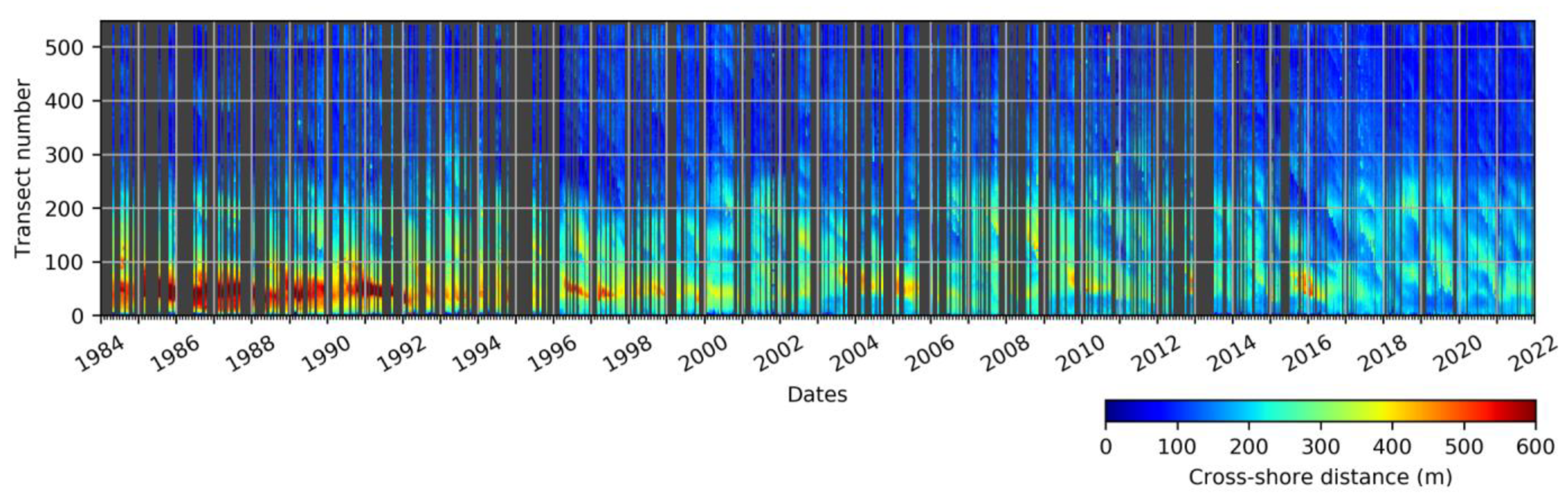
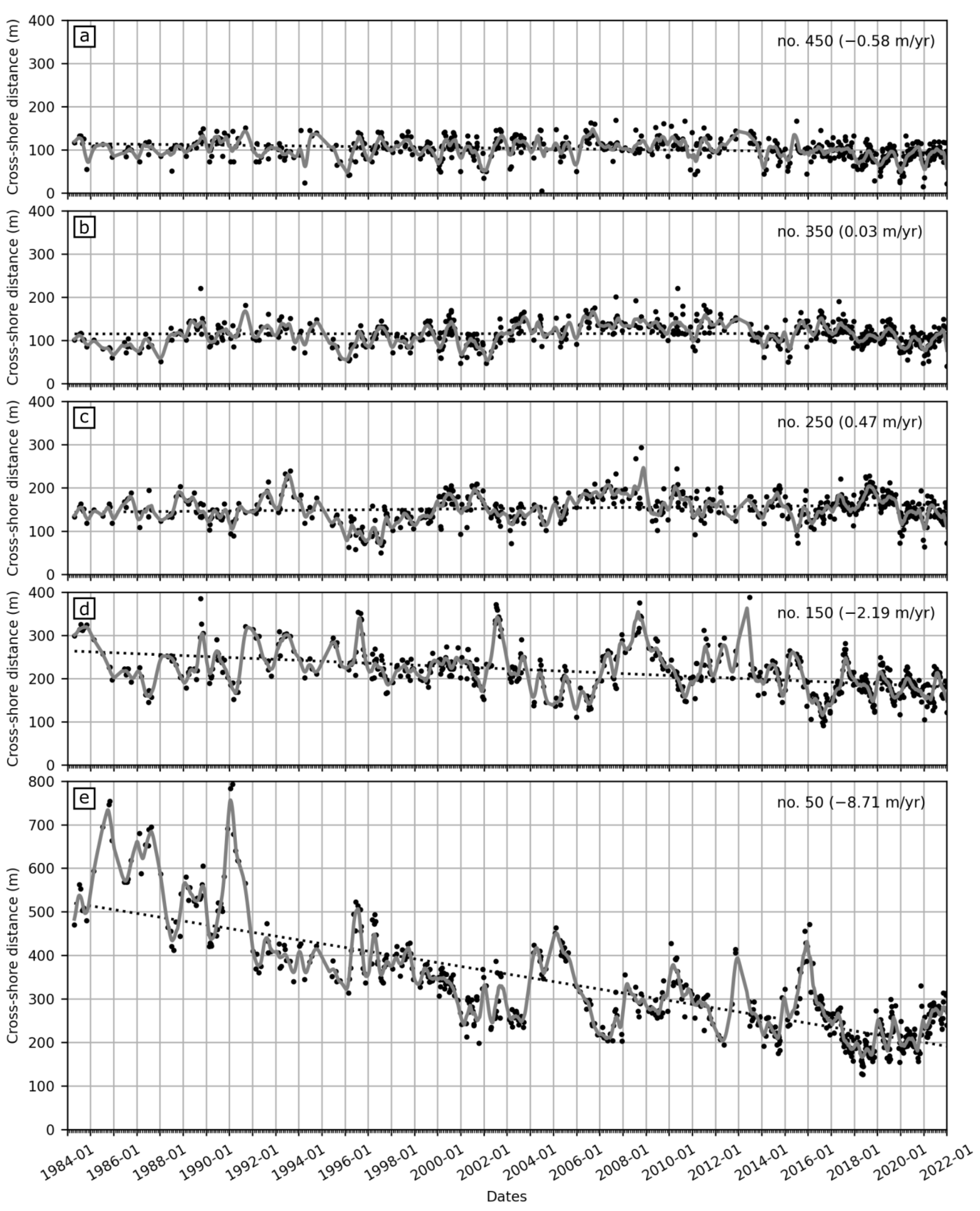
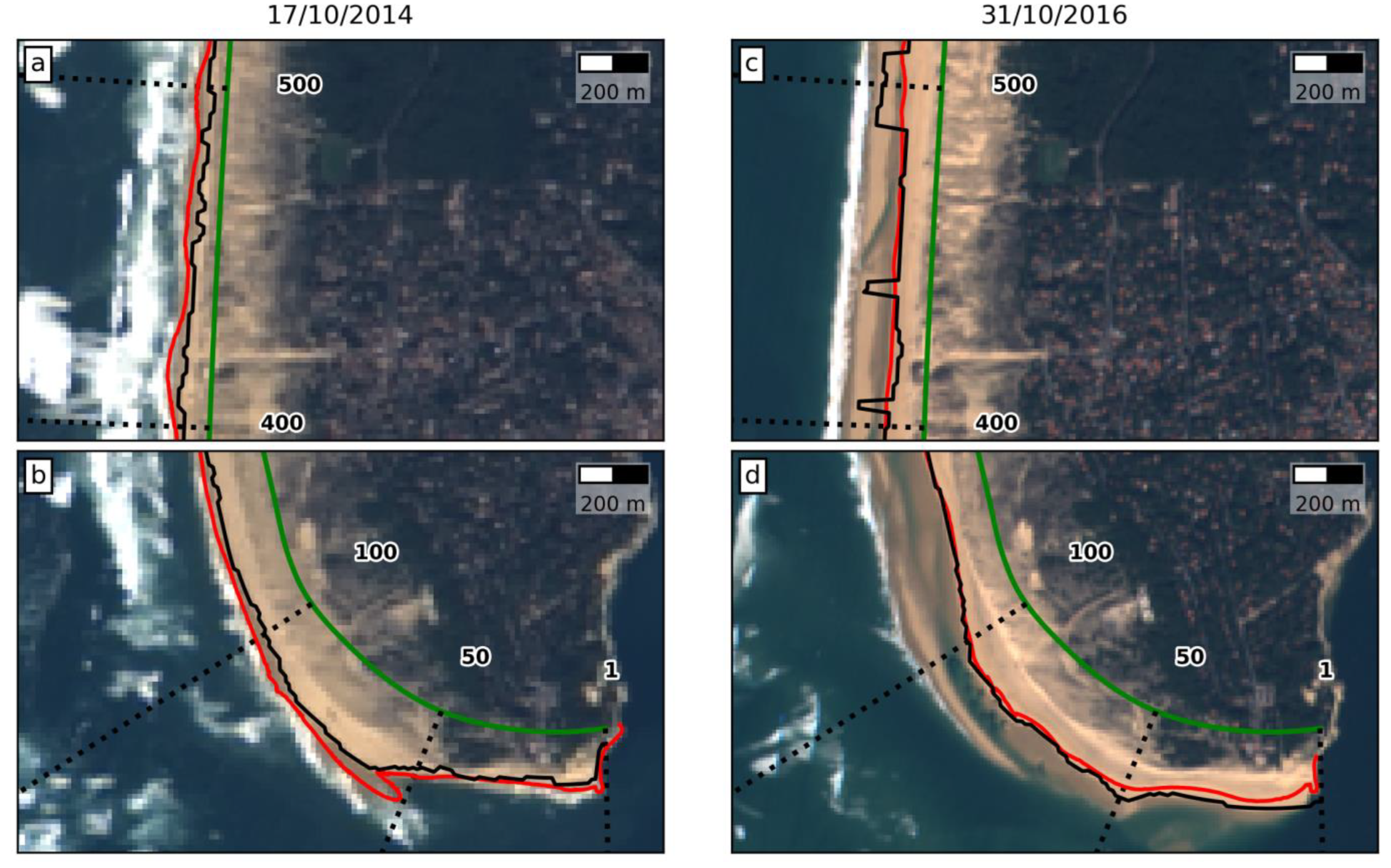
4.2. Spatiotemporal Evolution of Shoreline
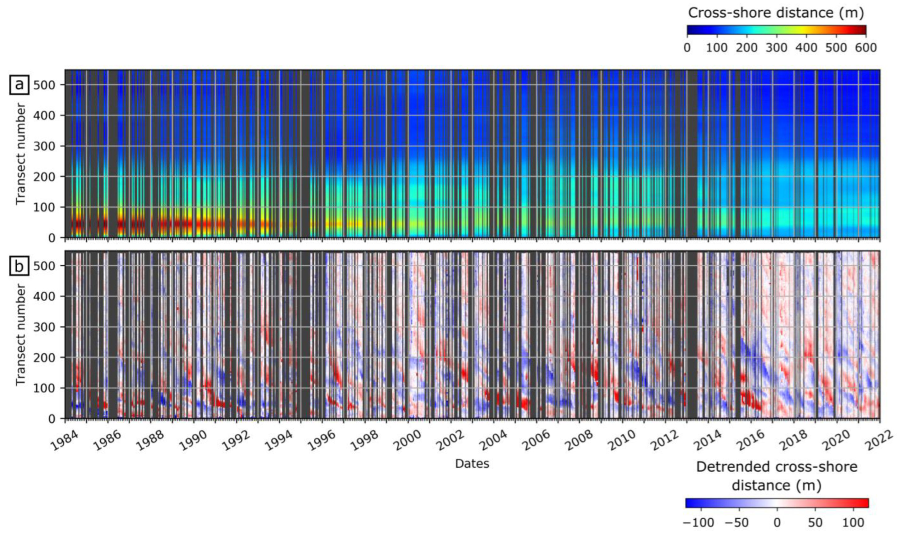
4.3. Migrating Shoreline Undulations
5. Discussion
5.1. Limitations and Advantages
5.2. Comparison with the Waterline-Based Shoreline Detection
5.3. Shoreline Variability Along the Cap Ferret Sand Spit
5.4. New Opportunities for Coastal Monitoring
6. Conclusions
Author Contributions
Funding
Data Availability Statement
Acknowledgments
Conflicts of Interest
Abbreviations
| CNES | Centre National des Etudes Spatiales |
| DTM | Digital Terrain Model |
| ESA | European Space Agency |
| GNSS | Global navigation satellite system |
| Hs | Significant wave height |
| IGN | Institut national de l’information Géographique et forestière (France) |
| LA | Landsat |
| MHW | Mean high water |
| MHWN | Mean high water neap |
| MSL | Mean sea level |
| NASA | National Aeronautics and Space Administration |
| NGF | Nivellement général de la France |
| no. | Number |
| n/a | Not applicable |
| RMSE | Root-mean-square error |
| R2 | Determination coefficient |
| SE | Sentinel |
| SDS | Satellite-derived shoreline |
| SP | SPOT |
| Tp | Peak wave period |
| USGS | United States Geological Survey |
References
- Stive, M.J.F.; Aarninkhof, S.G.J.; Hamm, L.; Hanson, H.; Larson, M.; Wijnberg, K.M.; Nicholls, R.J.; Capobianco, M. Variability of Shore and Shoreline Evolution. Coast. Eng. 2002, 47, 211–235. [Google Scholar] [CrossRef]
- Ashton, A.D.; Murray, A.B. High-angle Wave Instability and Emergent Shoreline Shapes: 2. Wave Climate Analysis and Comparisons to Nature. J. Geophys. Res. 2006, 111, F04012. [Google Scholar] [CrossRef]
- Harley, M.D.; Turner, I.L.; Short, A.D.; Ranasinghe, R. A Reevaluation of Coastal Embayment Rotation: The Dominance of Cross-Shore versus Alongshore Sediment Transport Processes, Collaroy-Narrabeen Beach, Southeast Australia. J. Geophys. Res. 2011, 116, F04033. [Google Scholar] [CrossRef]
- Castelle, B.; Marieu, V.; Bujan, S.; Splinter, K.D.; Robinet, A.; Sénéchal, N.; Ferreira, S. Impact of the Winter 2013–2014 Series of Severe Western Europe Storms on a Double-Barred Sandy Coast: Beach and Dune Erosion and Megacusp Embayments. Geomorphology 2015, 238, 135–148. [Google Scholar] [CrossRef]
- Pianca, C.; Holman, R.; Siegle, E. Shoreline Variability from Days to Decades: Results of Long-term Video Imaging. JGR Oceans 2015, 120, 2159–2178. [Google Scholar] [CrossRef]
- Bouvier, C.; Balouin, Y.; Castelle, B. Video Monitoring of Sandbar-Shoreline Response to an Offshore Submerged Structure at a Microtidal Beach. Geomorphology 2017, 295, 297–305. [Google Scholar] [CrossRef]
- Nicolae Lerma, A.; Castelle, B.; Marieu, V.; Robinet, A.; Bulteau, T.; Bernon, N.; Mallet, C. Decadal Beach-Dune Profile Monitoring along a 230-Km High-Energy Sandy Coast: Aquitaine, Southwest France. Appl. Geogr. 2022, 139, 102645. [Google Scholar] [CrossRef]
- Harley, M.D.; Turner, I.L.; Short, A.D. New Insights into Embayed Beach Rotation: The Importance of Wave Exposure and Cross-shore Processes. JGR Earth Surface 2015, 120, 1470–1484. [Google Scholar] [CrossRef]
- Castelle, B.; Guillot, B.; Marieu, V.; Chaumillon, E.; Hanquiez, V.; Bujan, S.; Poppeschi, C. Spatial and Temporal Patterns of Shoreline Change of a 280-Km High-Energy Disrupted Sandy Coast from 1950 to 2014: SW France. Estuar. Coast. Shelf Sci. 2018, 200, 212–223. [Google Scholar] [CrossRef]
- Vandenhove, M.; Castelle, B.; Nicolae Lerma, A.; Marieu, V.; Dalet, E.; Hanquiez, V.; Mazeiraud, V.; Bujan, S.; Mallet, C. Secular Shoreline Response to Large-Scale Estuarine Shoal Migration and Welding. Geomorphology 2024, 445, 108972. [Google Scholar] [CrossRef]
- Robinet, A.; Castelle, B.; Idier, D.; Le Cozannet, G.; Déqué, M.; Charles, E. Statistical Modeling of Interannual Shoreline Change Driven by North Atlantic Climate Variability Spanning 2000–2014 in the Bay of Biscay. Geo-Mar. Lett. 2016, 36, 479–490. [Google Scholar] [CrossRef]
- Robinet, A.; Castelle, B.; Idier, D.; Harley, M.D.; Splinter, K.D. Controls of Local Geology and Cross-Shore/Longshore Processes on Embayed Beach Shoreline Variability. Mar. Geol. 2020, 422, 106118. [Google Scholar] [CrossRef]
- Vitousek, S.; Barnard, P.L.; Limber, P.; Erikson, L.; Cole, B. A Model Integrating Longshore and Cross-shore Processes for Predicting Long-term Shoreline Response to Climate Change. JGR Earth Surface 2017, 122, 782–806. [Google Scholar] [CrossRef]
- Antolínez, J.A.A.; Méndez, F.J.; Anderson, D.; Ruggiero, P.; Kaminsky, G.M. Predicting Climate-Driven Coastlines with a Simple and Efficient Multiscale Model. JGR Earth Surface 2019, 124, 1596–1624. [Google Scholar] [CrossRef]
- Montaño, J.; Coco, G.; Antolínez, J.A.A.; Beuzen, T.; Bryan, K.R.; Cagigal, L.; Castelle, B.; Davidson, M.A.; Goldstein, E.B.; Ibaceta, R.; et al. Blind Testing of Shoreline Evolution Models. Sci. Rep. 2020, 10, 2137. [Google Scholar] [CrossRef]
- Boak, E.H.; Turner, I.L. Shoreline Definition and Detection: A Review. J. Coast. Res. 2005, 214, 688–703. [Google Scholar] [CrossRef]
- Hansen, J.E.; Barnard, P.L. Sub-Weekly to Interannual Variability of a High-Energy Shoreline. Coast. Eng. 2010, 57, 959–972. [Google Scholar] [CrossRef]
- Phillips, M.S.; Harley, M.D.; Turner, I.L.; Splinter, K.D.; Cox, R.J. Shoreline Recovery on Wave-Dominated Sandy Coastlines: The Role of Sandbar Morphodynamics and Nearshore Wave Parameters. Mar. Geol. 2017, 385, 146–159. [Google Scholar] [CrossRef]
- Yates, M.L.; Guza, R.T.; O’Reilly, W.C. Equilibrium Shoreline Response: Observations and Modeling. J. Geophys. Res. 2009, 114, C09014. [Google Scholar] [CrossRef]
- Castelle, B.; Marieu, V.; Bujan, S.; Ferreira, S.; Parisot, J.-P.; Capo, S.; Sénéchal, N.; Chouzenoux, T. Equilibrium Shoreline Modelling of a High-Energy Meso-Macrotidal Multiple-Barred Beach. Mar. Geol. 2014, 347, 85–94. [Google Scholar] [CrossRef]
- Vos, K.; Harley, M.D.; Splinter, K.D.; Simmons, J.A.; Turner, I.L. Sub-Annual to Multi-Decadal Shoreline Variability from Publicly Available Satellite Imagery. Coast. Eng. 2019, 150, 160–174. [Google Scholar] [CrossRef]
- Pardo-Pascual, J.E.; Almonacid-Caballer, J.; Ruiz, L.A.; Palomar-Vázquez, J. Automatic Extraction of Shorelines from Landsat TM and ETM+ Multi-Temporal Images with Subpixel Precision. Remote Sens. Environ. 2012, 123, 1–11. [Google Scholar] [CrossRef]
- Luijendijk, A.; Hagenaars, G.; Ranasinghe, R.; Baart, F.; Donchyts, G.; Aarninkhof, S. The State of the World’s Beaches. Sci. Rep. 2018, 8, 6641. [Google Scholar] [CrossRef]
- Vos, K.; Splinter, K.D.; Harley, M.D.; Simmons, J.A.; Turner, I.L. CoastSat: A Google Earth Engine-Enabled Python Toolkit to Extract Shorelines from Publicly Available Satellite Imagery. Environ. Model. Softw. 2019, 122, 104528. [Google Scholar] [CrossRef]
- Sánchez-García, E.; Palomar-Vázquez, J.M.; Pardo-Pascual, J.E.; Almonacid-Caballer, J.; Cabezas-Rabadán, C.; Gómez-Pujol, L. An Efficient Protocol for Accurate and Massive Shoreline Definition from Mid-Resolution Satellite Imagery. Coast. Eng. 2020, 160, 103732. [Google Scholar] [CrossRef]
- Almeida, L.P.; Efraim de Oliveira, I.; Lyra, R.; Scaranto Dazzi, R.L.; Martins, V.G.; Henrique da Fontoura Klein, A. Coastal Analyst System from Space Imagery Engine (CASSIE): Shoreline Management Module. Environ. Model. Softw. 2021, 140, 105033. [Google Scholar] [CrossRef]
- Mao, Y.; Harris, D.L.; Xie, Z.; Phinn, S. Efficient Measurement of Large-Scale Decadal Shoreline Change with Increased Accuracy in Tide-Dominated Coastal Environments with Google Earth Engine. ISPRS J. Photogramm. Remote Sens. 2021, 181, 385–399. [Google Scholar] [CrossRef]
- Castelle, B.; Masselink, G.; Scott, T.; Stokes, C.; Konstantinou, A.; Marieu, V.; Bujan, S. Satellite-Derived Shoreline Detection at a High-Energy Meso-Macrotidal Beach. Geomorphology 2021, 383, 107707. [Google Scholar] [CrossRef]
- Warrick, J.A.; Vos, K.; Buscombe, D.; Ritchie, A.C.; Curtis, J.A. A Large Sediment Accretion Wave Along a Northern California Littoral Cell. JGR Earth Surface 2023, 128, e2023JF007135. [Google Scholar] [CrossRef]
- Mentaschi, L.; Vousdoukas, M.I.; Pekel, J.-F.; Voukouvalas, E.; Feyen, L. Global Long-Term Observations of Coastal Erosion and Accretion. Sci. Rep. 2018, 8, 12876. [Google Scholar] [CrossRef]
- Serafin, K.A.; Ruggiero, P. Simulating Extreme Total Water Levels Using a Time-dependent, Extreme Value Approach. JGR Oceans 2014, 119, 6305–6329. [Google Scholar] [CrossRef]
- Komar, P.D.; Enfield, D.B. Short-term sea-level changes and coastal erosion. In Sea Level Fluctuation and Coastal Evolution; Nummedal, D., Pilkey, O.H., Howard, J.D., Eds.; Society of Economic Paleontologists and Mineralogists: Tulsa, OK, USA, 1987; Volume 41, pp. 17–27. [Google Scholar]
- García-Rubio, G.; Huntley, D.; Russell, P. Evaluating Shoreline Identification Using Optical Satellite Images. Mar. Geol. 2015, 359, 96–105. [Google Scholar] [CrossRef]
- Bishop-Taylor, R.; Nanson, R.; Sagar, S.; Lymburner, L. Mapping Australia’s Dynamic Coastline at Mean Sea Level Using Three Decades of Landsat Imagery. Remote Sens. Environ. 2021, 267, 112734. [Google Scholar] [CrossRef]
- Vos, K.; Splinter, K.D.; Palomar-Vázquez, J.; Pardo-Pascual, J.E.; Almonacid-Caballer, J.; Cabezas-Rabadán, C.; Kras, E.C.; Luijendijk, A.P.; Calkoen, F.; Almeida, L.P.; et al. Benchmarking Satellite-Derived Shoreline Mapping Algorithms. Commun. Earth Environ. 2023, 4, 345. [Google Scholar] [CrossRef]
- Vitousek, S.; Vos, K.; Splinter, K.D.; Erikson, L.; Barnard, P.L. A Model Integrating Satellite-Derived Shoreline Observations for Predicting Fine-Scale Shoreline Response to Waves and Sea-Level Rise Across Large Coastal Regions. JGR Earth Surface 2023, 128, e2022JF006936. [Google Scholar] [CrossRef]
- van der Werff, H.M.A. Mapping Shoreline Indicators on a Sandy Beach with Supervised Edge Detection of Soil Moisture Differences. Int. J. Appl. Earth Obs. Geoinf. 2019, 74, 231–238. [Google Scholar] [CrossRef]
- McBeth, F.H. A Method of Shoreline Delineation. Photogramm. Eng. 1956, 22, 21–25. [Google Scholar]
- Dolan, R.; Hayden, B.; Heywood, J. A New Photogrammetric Method for Determining Shoreline Erosion. Coast. Eng. 1978, 2, 21–39. [Google Scholar] [CrossRef]
- Pajak, M.J.; Leatherman, S. The High Water Line as Shoreline Indicator. J. Coast. Res. 2022, 18, 329–337. [Google Scholar]
- Vicens-Miquel, M.; Medrano, F.A.; Tissot, P.E.; Kamangir, H.; Starek, M.J.; Colburn, K. A Deep Learning Based Method to Delineate the Wet/Dry Shoreline and Compute Its Elevation Using High-Resolution UAS Imagery. Remote Sens. 2022, 14, 5990. [Google Scholar] [CrossRef]
- McAllister, E.; Payo, A.; Novellino, A.; Dolphin, T.; Medina-Lopez, E. Multispectral Satellite Imagery and Machine Learning for the Extraction of Shoreline Indicators. Coast. Eng. 2022, 174, 104102. [Google Scholar] [CrossRef]
- Pardo-Pascual, J.E.; Almonacid-Caballer, J.; Cabezas-Rabadán, C.; Fernández-Sarría, A.; Armaroli, C.; Ciavola, P.; Montes, J.; Souto-Ceccon, P.E.; Palomar-Vázquez, J. Assessment of Satellite-Derived Shorelines Automatically Extracted from Sentinel-2 Imagery Using SAET. Coast. Eng. 2024, 188, 104426. [Google Scholar] [CrossRef]
- Sekovski, I.; Stecchi, F.; Mancini, F.; Del Rio, L. Image Classification Methods Applied to Shoreline Extraction on Very High-Resolution Multispectral Imagery. Int. J. Remote Sens. 2014, 35, 3556–3578. [Google Scholar] [CrossRef]
- Ollerhead, J.; Davidson-Arnott, R.G.D. The Evolution of Buctouche Spit, New Brunswick, Canada. Mar. Geol. 1995, 124, 215–236. [Google Scholar] [CrossRef]
- Simeoni, U.; Fontolan, G.; Tessari, U.; Corbau, C. Domains of Spit Evolution in the Goro Area, Po Delta, Italy. Geomorphology 2007, 86, 332–348. [Google Scholar] [CrossRef]
- Allard, J.; Bertin, X.; Chaumillon, E.; Pouget, F. Sand Spit Rhythmic Development: A Potential Record of Wave Climate Variations? Arçay Spit, Western Coast of France. Mar. Geol. 2008, 253, 107–131. [Google Scholar] [CrossRef]
- Dan, S.; Stive, M.J.F.; Walstra, D.-J.R.; Panin, N. Wave Climate, Coastal Sediment Budget and Shoreline Changes for the Danube Delta. Mar. Geol. 2009, 262, 39–49. [Google Scholar] [CrossRef]
- Evans, O.F. The Origin of Spits, Bars, and Related Structures. J. Geol. 1942, 50, 846–865. [Google Scholar]
- Petersen, D.; Deigaard, R.; Fredsøe, J. Modelling the Morphology of Sandy Spits. Coast. Eng. 2008, 55, 671–684. [Google Scholar] [CrossRef]
- Bertin, X.; Deshouilieres, A.; Allard, J.; Chaumillon, E. A New Fluorescent Tracers Experiment Improves Understanding of Sediment Dynamics along the Arcay Sandspit (France). Geo-Mar. Lett. 2007, 27, 63–69. [Google Scholar] [CrossRef]
- Anthony, E.J. Wave Influence in the Construction, Shaping and Destruction of River Deltas: A Review. Mar. Geol. 2015, 361, 53–78. [Google Scholar] [CrossRef]
- Robin, N.; Levoy, F.; Anthony, E.J.; Monfort, O. Sand Spit Dynamics in a Large Tidal-range Environment: Insight from Multiple LiDAR, UAV and Hydrodynamic Measurements on Multiple Spit Hook Development, Breaching, Reconstruction, and Shoreline Changes. Earth Surf. Process. Landf. 2020, 45, 2706–2726. [Google Scholar] [CrossRef]
- Nahon, A.; Idier, D.; Bertin, X.; Guérin, T.; Marieu, V.; Sénéchal, N.; Mugica, J. Modelling the Contribution of Wind Waves to Cap Ferret’s Updrift Erosion. Coast. Eng. 2022, 172, 104063. [Google Scholar] [CrossRef]
- Nahon, A.; Idier, D.; Sénéchal, N.; Féniès, H.; Mallet, C.; Mugica, J. Imprints of Wave Climate and Mean Sea Level Variations in the Dynamics of a Coastal Spit over the Last 250 Years: Cap Ferret, SW France. Earth Surf. Process. Landf. 2019, 44, 2112–2125. [Google Scholar] [CrossRef]
- Pringle, A.W. Holderness Coast Erosion and the Significance of Ords. Earth Surf. Process. Landf. 1985, 10, 107–124. [Google Scholar] [CrossRef]
- Stewart, C.J.; Davidson-Arnott, R.G.D. Morphology, Formation and Migration of Longshore Sandwaves; Long Point, Lake Erie, Canada. Mar. Geol. 1988, 81, 63–77. [Google Scholar] [CrossRef]
- Davidson-Arnott, R.G.D.; Van Heyningen, A.G. Migration and Sedimentology of Longshore Sandwaves, Long Point, Lake Erie, Canada. Sedimentology 2003, 50, 1123–1137. [Google Scholar] [CrossRef]
- Medellín, G.; Medina, R.; Falqués, A.; González, M. Coastline Sand Waves on a Low-Energy Beach at “El Puntal” Spit, Spain. Mar. Geol. 2008, 250, 143–156. [Google Scholar] [CrossRef]
- López-Ruiz, A.; Ortega-Sánchez, M.; Baquerizo, A.; Losada, M.A. Short and Medium-Term Evolution of Shoreline Undulations on Curvilinear Coasts. Geomorphology 2012, 159–160, 189–200. [Google Scholar] [CrossRef]
- Ashton, A.D.; Nienhuis, J.; Ells, K. On a Neck, on a Spit: Controls on the Shape of Free Spits. Earth Surf. Dynam. 2016, 4, 193–210. [Google Scholar] [CrossRef]
- Taveneau, A.; Almar, R.; Bergsma, E.W.J.; Sy, B.A.; Ndour, A.; Sadio, M.; Garlan, T. Observing and Predicting Coastal Erosion at the Langue de Barbarie Sand Spit around Saint Louis (Senegal, West Africa) through Satellite-Derived Digital Elevation Model and Shoreline. Remote Sens. 2021, 13, 2454. [Google Scholar] [CrossRef]
- Taveneau, A.; Almar, R.; Bergsma, E.W.J. On the Cyclic Behavior of Wave-Driven Sandspits with Implications for Coastal Zone Management. Estuar. Coast. Shelf Sci. 2024, 303, 108798. [Google Scholar] [CrossRef]
- Féniès, H.; Lericolais, G. Architecture Interne d’une Vallée Incisée Sur Une Côte à Forte Énergie de Houle et de Marée (Vallée de La Leyre, Côte Aquitaine, France). Comptes Rendus. Géosci. 2005, 337, 1257–1266. [Google Scholar] [CrossRef]
- Allard, J.; Chaumillon, E.; Féniès, H. A Synthesis of Morphological Evolutions and Holocene Stratigraphy of a Wave-Dominated Estuary: The Arcachon Lagoon, SW France. Cont. Shelf Res. 2009, 29, 957–969. [Google Scholar] [CrossRef]
- Idier, D.; Castelle, B.; Charles, E.; Mallet, C. Longshore Sediment Flux Hindcast: Spatio-Temporal Variability along the SW Atlantic Coast of France. J. Coast. Res. 2013, 165, 1785–1790. [Google Scholar] [CrossRef]
- Castelle, B.; Dodet, G.; Masselink, G.; Scott, T. A New Climate Index Controlling Winter Wave Activity along the Atlantic Coast of Europe: The West Europe Pressure Anomaly. Geophys. Res. Lett. 2017, 44, 1384–1392. [Google Scholar] [CrossRef]
- Castelle, B.; Bujan, S.; Ferreira, S.; Dodet, G. Foredune Morphological Changes and Beach Recovery from the Extreme 2013/2014 Winter at a High-Energy Sandy Coast. Mar. Geol. 2017, 385, 41–55. [Google Scholar] [CrossRef]
- Salles, P.; Valle-Levinson, A.; Sottolichio, A.; Senechal, N. Wind-driven Modifications to the Residual Circulation in an Ebb-tidal Delta: Arcachon L Agoon, S Outhwestern F Rance. JGR Oceans 2015, 120, 728–740. [Google Scholar] [CrossRef]
- Gallagher, E.L.; MacMahan, J.; Reniers, A.J.H.M.; Brown, J.; Thornton, E.B. Grain Size Variability on a Rip-Channeled Beach. Mar. Geol. 2011, 287, 43–53. [Google Scholar] [CrossRef]
- Nahon, A. Évolution Morphologique Actuelle d’une Flèche Littorale Holocène: Le Cap Ferret, à L’embouchure du Bassin d’Arcachon. Thèse de Doctorat, Université de Bordeaux, Bordeaux, France, 2018. [Google Scholar]
- Bossard, V.; Nicolae Lerma, A. Geomorphologic Characteristics and Evolution of Managed Dunes on the South West Coast of France. Geomorphology 2020, 367, 107312. [Google Scholar] [CrossRef]
- Castelle, B.; Bonneton, P.; Dupuis, H.; Sénéchal, N. Double Bar Beach Dynamics on the High-Energy Meso-Macrotidal French Aquitanian Coast: A Review. Mar. Geol. 2007, 245, 141–159. [Google Scholar] [CrossRef]
- Lafon, V.; De Melo Apoluceno, D.; Dupuis, H.; Michel, D.; Howa, H.; Froidefond, J.M. Morphodynamics of Nearshore Rhythmic Sandbars in a Mixed-Energy Environment (SW France): I. Mapping Beach Changes Using Visible Satellite Imagery. Estuar. Coast. Shelf Sci. 2004, 61, 289–299. [Google Scholar] [CrossRef]
- Dubarbier, B.; Castelle, B.; Ruessink, G.; Marieu, V. Mechanisms Controlling the Complete Accretionary Beach State Sequence. Geophys. Res. Lett. 2017, 44, 5645–5654. [Google Scholar] [CrossRef]
- Thornton, E.B.; MacMahan, J.; Sallenger, A.H. Rip Currents, Mega-Cusps, and Eroding Dunes. Mar. Geol. 2007, 240, 151–167. [Google Scholar] [CrossRef]
- Castelle, B.; Marieu, V.; Bujan, S. Alongshore-Variable Beach and Dune Changes on the Timescales from Days (Storms) to Decades Along the Rip-Dominated Beaches of the Gironde Coast, SW France. J. Coast. Res. 2019, 88, 157–171. [Google Scholar] [CrossRef]
- Castelle, B.; Bujan, S.; Marieu, V.; Ferreira, S. 16 Years of Topographic Surveys of Rip-Channelled High-Energy Meso-Macrotidal Sandy Beach. Sci. Data 2020, 7, 410. [Google Scholar] [CrossRef]
- Gassiat, L. Hydrodynamique et Evolution Sédimentaire d’un Système Lagune-Flèche Littorale. Le Bassin d’Arcachon et la Flèche du Cap Ferret. Thèse de Doctorat, Université de Bordeaux, Bordeaux, France, 1989. [Google Scholar]
- Castelle, B.; Ritz, A.; Marieu, V.; Nicolae Lerma, A.; Vandenhove, M. Primary Drivers of Multidecadal Spatial and Temporal Patterns of Shoreline Change Derived from Optical Satellite Imagery. Geomorphology 2022, 413, 108360. [Google Scholar] [CrossRef]
- Bernon, N.; Mallet, C.; Belon, R. Caractérisation de l’aléa Recul Du trait de côte sur le Littoral de la côte Aquitaine aux Horizons 2025 et 2050; BRGM: Pessac, France, 2016. [Google Scholar]
- Bernon, N.; Mallet, C. Synthèse de L’accompagnement de l’Observatoire de la Côte Aquitaine dans la Gestion de L’érosion du Cordon Dunaire à la Pointe du Cap Ferret-Hiver 2017/2018; BRGM: Pessac, France, 2018. [Google Scholar]
- Gorelick, N.; Hancher, M.; Dixon, M.; Ilyushchenko, S.; Thau, D.; Moore, R. Google Earth Engine: Planetary-Scale Geospatial Analysis for Everyone. Remote Sens. Environ. 2017, 202, 18–27. [Google Scholar] [CrossRef]
- Rabaute, T.; Tinel, C.; Marzocchi-Polizzi, S.; De Boissezon, H. Kalideos, Des Images Pour La Science: Un Instrument Au Service Des Applications Thématiques. RFPT 2012, 197, 3–9. [Google Scholar] [CrossRef]
- Nicolae Lerma, A.; Ayache, B.; Ulvoas, B.; Paris, F.; Bernon, N.; Bulteau, T.; Mallet, C. Pluriannual Beach-Dune Evolutions at Regional Scale: Erosion and Recovery Sequences Analysis along the Aquitaine Coast Based on Airborne LiDAR Data. Cont. Shelf Res. 2019, 189, 103974. [Google Scholar] [CrossRef]
- Pedregosa, F.; Varoquaux, G.; Gramfort, A.; Michel, V.; Thirion, B.; Grisel, O.; Blondel, M.; Prettenhofer, P.; Weiss, R.; Dubourg, V.; et al. Scikit-Learn: Machine Learning in Python. J. Mach. Learn. Res. 2011, 12, 2825–2830. [Google Scholar]
- Gao, B. NDWI—A Normalized Difference Water Index for Remote Sensing of Vegetation Liquid Water from Space. Remote Sens. Environ. 1996, 58, 257–266. [Google Scholar] [CrossRef]
- Xu, H. Modification of Normalised Difference Water Index (NDWI) to Enhance Open Water Features in Remotely Sensed Imagery. Int. J. Remote Sens. 2006, 27, 3025–3033. [Google Scholar] [CrossRef]
- Stockdon, H.F.; Holman, R.A.; Howd, P.A.; Sallenger, A.H. Empirical Parameterization of Setup, Swash, and Runup. Coast. Eng. 2006, 53, 573–588. [Google Scholar] [CrossRef]
- Konstantinou, A.; Scott, T.; Masselink, G.; Stokes, K.; Conley, D.; Castelle, B. Satellite-Based Shoreline Detection along High-Energy Macrotidal Coasts and Influence of Beach State. Mar. Geol. 2023, 462, 107082. [Google Scholar] [CrossRef]
- FitzGerald, D.M. Sediment Bypassing at Mixed Energy Tidal Inlets. In Proceedings of the Coastal Engineering 1982; American Society of Civil Engineers: Cape Town, South Africa, 1982; pp. 1094–1118. [Google Scholar]
- Elias, E.P.L.; Van der Spek, A.J.F.; Pearson, S.G.; Cleveringa, J. Understanding Sediment Bypassing Processes through Analysis of High-Frequency Observations of Ameland Inlet, the Netherlands. Mar. Geol. 2019, 415, 105956. [Google Scholar] [CrossRef]
- Ashton, A.D.; Murray, A.B. High-angle Wave Instability and Emergent Shoreline Shapes: 1. Modeling of Sand Waves, Flying Spits, and Capes. J. Geophys. Res. 2006, 111, 2005JF000422. [Google Scholar] [CrossRef]
- Medellín, G.; Falqués, A.; Medina, R.; González, M. Coastline Sand Waves on a Low-energy Beach at El Puntal Spit, Spain: Linear Stability Analysis. J. Geophys. Res. 2009, 114, C03022. [Google Scholar] [CrossRef]


| Blue | Green | Red | Near-Infrared | Short Wave Infrared | Panchromatic | |
|---|---|---|---|---|---|---|
| Landsat 5 | 30—band 1 | 30—band 2 | 30—band 3 | 30—band 4 | 30—band 5 | - |
| Landsat 7 | 30—band 1 | 30—band 2 | 30—band 3 | 30—band 4 | 30—band 5 | 15—band 8 |
| Landsat 8 | 30—band 2 | 30—band 3 | 30—band 4 | 30—band 5 | 30—band 6 | 15—band 8 |
| Sentinel-2 | 10—band 2 | 10—band 3 | 10—band 4 | 10—band 8 | 20—band 11 | - |
| SPOT 1/2 | - | 20—band 1 | 20—band 2 | 20—band 3 | - | - |
| SPOT 4 | - | 20—band 1 | 20—band 2 | 20—band 3 | 20—band 4 | 10—band 5 * |
| SPOT 5 | - | 10—band 1 | 10—band 2 | 10—band 3 | 20—band 4 | - |
| Name | Urbanized Area and Dense Vegetation | Vegetated Dune | Dry Sand | Slightly Wet Sand | Very Wet Sand | Breaking Waves and Foam | Shallow Water | Deep Water |
|---|---|---|---|---|---|---|---|---|
| Value | 1 | 2 | 3 | 4 | 5 | 6 | 7 | 8 |
| Site [Study] | Detection Based on | Tidal Range (m) | Target Datum- Based Shoreline | Water Level Correction | Image Exclusion | RMSE (m) | Bias (m) | R2 | n |
|---|---|---|---|---|---|---|---|---|---|
| Cap Ferret sand spit [this work] | wet/dry line | 3.8 | MHW | none | none | 20.2 | 1.7 | 0.86 | 11 |
| Truc Vert [28] | waterline (CoastSat) | 3.7 | MHW | none | none | 31.4 | 22.5 | 0.42 | 226 |
| tide-only | none | 15.6 | −8.0 | 0.53 | 226 | ||||
| tide and wave runup | low-tide images | 10.3 | 7.1 | 0.78 | 164 | ||||
| Slapton Sands [90] | waterline (CoastSat) | 4.4 | MHW | none | none | 18.1 | 10.2 | n/a | 147 |
| tide-only | none | 14.0 | 6.5 | n/a | 147 | ||||
| Perranporth [90] | waterline (CoastSat) | 6.3 | MHWN | none | none | 138.2 | 16.2 | n/a | 93 |
| tide and wave runup | none | 22.2 | −4.2 | n/a | 93 |
Disclaimer/Publisher’s Note: The statements, opinions and data contained in all publications are solely those of the individual author(s) and contributor(s) and not of MDPI and/or the editor(s). MDPI and/or the editor(s) disclaim responsibility for any injury to people or property resulting from any ideas, methods, instructions or products referred to in the content. |
© 2025 by the authors. Licensee MDPI, Basel, Switzerland. This article is an open access article distributed under the terms and conditions of the Creative Commons Attribution (CC BY) license (https://creativecommons.org/licenses/by/4.0/).
Share and Cite
Robinet, A.; Bernon, N.; Nicolae Lerma, A. Multi-Decadal Shoreline Variability Along the Cap Ferret Sand Spit (SW France) Derived from Satellite Images. Remote Sens. 2025, 17, 1200. https://doi.org/10.3390/rs17071200
Robinet A, Bernon N, Nicolae Lerma A. Multi-Decadal Shoreline Variability Along the Cap Ferret Sand Spit (SW France) Derived from Satellite Images. Remote Sensing. 2025; 17(7):1200. https://doi.org/10.3390/rs17071200
Chicago/Turabian StyleRobinet, Arthur, Nicolas Bernon, and Alexandre Nicolae Lerma. 2025. "Multi-Decadal Shoreline Variability Along the Cap Ferret Sand Spit (SW France) Derived from Satellite Images" Remote Sensing 17, no. 7: 1200. https://doi.org/10.3390/rs17071200
APA StyleRobinet, A., Bernon, N., & Nicolae Lerma, A. (2025). Multi-Decadal Shoreline Variability Along the Cap Ferret Sand Spit (SW France) Derived from Satellite Images. Remote Sensing, 17(7), 1200. https://doi.org/10.3390/rs17071200