Spaceborne GNSS Reflectometry for Vegetation and Inland Water Monitoring: Progress, Challenges, Opportunities, and Potential

Abstract

Global navigation satellite system reflectometry (GNSS-R) uses the reflection characteristics of navigation satellite signals reflected from the earth’s surface to provide an innovative tool for remote sensing, especially for monitoring surface and atmospheric environmental variables, such as wind speed, soil moisture, vegetation, and sea ice parameters. This paper focuses on the current application and future potential of spaceborne GNSS-R in vegetation remote sensing and the retrieval of inland water environmental and physical parameters. This paper reviews the technical progress of GNSS-R in detail, from early feasibility studies to multiple application examples at this stage, from the United Kingdom Disaster Monitoring Constellation (UK-DMC) satellite in 2003 to other recent GNSS-R missions. These cases demonstrate the unique advantages of GNSS-R in terms of global coverage, low cost, and real-time monitoring. This paper explores the application of GNSS-R technology in vegetation parameters and inland water monitoring, especially its potential in vegetation parameters and surface water monitoring applications. The article also mentioned that the accuracy and efficiency of parameter retrieval can be significantly improved by improving models and algorithms, such as using neural networks and data fusion technology. Finally, the article points out the future direction of spaceborne GNSS-R technology in vegetation remote sensing and the retrieval of inland water environment and physical parameters, including expanding its application areas to a broader range of environmental monitoring and resource management. It emphasized its essential role in monitoring the global ecosystem and monitoring water resources.

1. Introduction

Vegetation and inland water bodies are important to the Earth’s ecosystem. Vegetation is a key factor in combating global warming through photosynthesis, which absorbs carbon dioxide and releases oxygen [1]. The health of plants also reflects the impact of environmental pressures such as land use changes, pests and diseases, and climate change. Inland water bodies significantly impact water security, agricultural irrigation, and others [2]. In addition, there is a close link between the environmental and the physical parameters of vegetation and inland water bodies: vegetation affects the evaporation and infiltration processes of water bodies, which leads to changes in water levels and others [3], and water bodies also have an impact on the growth and development of plants [4]. Together, these parameters characterize and affect the ecology of the region. Monitoring these natural elements is challenging because the areas to be monitored are often remote, which makes the monitoring process difficult and expensive. This requires the use of remote sensing technology, especially spaceborne global navigation satellite system reflectometry (GNSS-R) technology, to obtain information about water distribution [5], vegetation water content (VWC) [6], and canopy height (CH) [7] by analyzing the reflection of satellite signals on the Earth’s surface, providing strong scientific and technological support for environmental protection and resource management.

In recent years, GNSS-R technology has developed rapidly in the field of environmental and physical parameters of inland water bodies and vegetation parameters. Compared with traditional remote sensing technology, spaceborne GNSS-R has the unique advantages of low cost, real-time monitoring [8], and high resolution while also exhibiting strong anti-interference capabilities [6]. In [9,10], they review the progress in applying GNSS-R in monitoring, especially its vital role in predicting the risk of strong winds, floods, ocean eddies, and storm surges. Camps et al. [11] reviewed the application progress of GNSS-R technology in land monitoring, especially its potential to monitor soil moisture, surface topography, water levels, vegetation, and snow height. By reflecting GNSS signals, this technology demonstrates high spatial resolution and anti-interference ability and is suitable for monitoring various environments. Yu et al. [12] summarized GNSS-R or GNSS transmission (GNSS-T) opportunity signal technology used to measure geographical parameters such as soil moisture, surface topography, water levels, vegetation, snow height, and VWC. Yan and Huang [13] summarized the GNSS-R sea ice remote sensing methods, including applications such as sea ice detection, sea ice concentration estimation, sea ice type classification, sea ice thickness retrieval, and sea ice altimetry. They also demonstrated the potential of GNSS-R technology for high precision and spatial resolution. Edokossi et al. [14] reviewed using GNSS-R technology to measure soil moisture content (SMC) and demonstrated the advantages of GNSS-R technology in global coverage, low cost, and real-time monitoring. In [15,16], they reviewed the progress of GNSS-R in soil moisture monitoring, vegetation monitoring, polarization, and coherent and incoherent scattering and pointed out that the current algorithm relies on auxiliary data, and the independent retrieval capability needs to be improved. In vegetation remote sensing, the focus is on analyzing the impact of GNSS-R multi-angle observation and polarization characteristics on vegetation monitoring, pointing out the shortcomings of existing models in polarization and geometric angle processing, and emphasizing the necessity of improving retrieval accuracy through theoretical models. Carreno-Luengo et al. [17] reviewed the application of GNSS-R technology in the remote sensing of ocean, land, and cryosphere. The application potential of GNSS-R technology in retrieving parameters such as ocean wind speed, sea surface height, soil moisture, and biomass was highlighted. However, it also faces challenges such as low data spatial resolution and radio frequency interference (RFI). Euriques et al. [18] analyzed the advantages of using GNSS-R technology for soil moisture estimation, such as wide coverage, low cost, and no climate impact. However, this technology still faces the challenge of retrieval accuracy, which is affected by topography, vegetation, surface roughness, and soil temperature. It is pointed out that the accuracy of GNSS-R soil moisture estimation can be improved by improving models and data fusion. Unwin et al. [19] introduced using HydroGNSS mission GNSS-R data to monitor hydrological-related climate variables, including soil moisture, wetland cover, freeze–thaw status, and aboveground biomass. The potential of providing high-resolution, low-cost global observation data through small satellite constellations is pointed out. Pierdicca et al. [20] explored the potential application of spaceborne GNSS-R in soil moisture, biomass, and freeze–thaw monitoring. The study set three goals: first, to verify the predictive ability of current models and ground experiments in soil moisture and vegetation biomass retrieval; second, to understand the impact of freeze–thaw dynamics and other biophysical phenomena on reflected signals; and third, to improve the retrieval algorithm based on neural networks to further improve the retrieval accuracy and the breadth of practical applications. In [21,22], they pointed out that vegetation monitoring mainly focuses on qualitative analysis and the application of satellite observation data. Future research will focus on exploring observation geometry and polarimetric data, seeking the best observation combination, and promoting the development of quantitative retrieval technology. Bu et al. [23] reviewed the potential applications of GNSS-R on land. He emphasized the need to develop more advanced GNSS-R modeling algorithms and optimize the design of next-generation instruments to improve their performance. Yang et al. [24] reviewed the application of GNSS-R technology in soil moisture retrieval, discussed the principles and research status of technologies based on different platforms (ground-based, airborne, and spaceborne), pointed out that the introduction of transfer learning and spatial feature fusion methods is expected to improve the retrieval accuracy, and emphasized the potential of machine learning (ML) and deep learning (DL) in parameter monitoring.

Spaceborne GNSS-R technology has shown enormous potential for land remote sensing applications. With its advantages of accurately measuring key geographical parameters, such as soil moisture, water levels, topography, vegetation cover, and soil freeze–thaw conditions, and its low cost, strong anti-interference, and high spatial resolution, this technology has become exceedingly popular in environmental monitoring. However, despite the broad prospects, some challenges remain, such as interference from non-target parameters, improving retrieval accuracy, optimizing data quality, and further improving modeling algorithms. Most of the current literature focuses on the research of GNSS-R technology in specific application fields. However, there is a relative lack of systematic reviews on the comprehensive application of this technology in monitoring the environmental and physical parameters of inland water bodies and vegetation and the challenges it faces. This review focuses on analyzing the progress of GNSS-R technology in monitoring environmental, physical, and vegetation parameters in inland water bodies and the main challenges it faces. The two fields are interrelated in ecosystem monitoring. Water bodies and vegetation are among the most critical elements of the Earth’s ecosystem, and their state directly affects key ecological functions such as the hydrological cycle, climate regulation, and biodiversity. Therefore, this paper aims to review and analyze the progress of spaceborne GNSS-R technology in these fields, focusing on its innovative prospects for vegetation monitoring and the physical parameters of inland water environments to provide a reference for the future development of the technology and deeper insights.

The structure of the rest of this article is as follows: In Section 2, we briefly introduced the current development status of the spaceborne GNSS-R microsatellites constellation. Section 3 studied the various applications of GNSS-R technology in the field of vegetation, including the assessment of vegetation water content, vegetation optical depth (VOD), and the observation of forest AGB and CH. In this process, this section emphasizes the importance of this technology in promoting ecological protection. Section 4 provides an overview of methods for retrieving the physical parameters of inland water bodies, including inland water body detection, water level monitoring, river width, slope measurements, as well as surface wind speed and wave height estimation. The advantages and disadvantages of various methods are analyzed. Section 5 focuses on the methods of retrieving environmental parameters of inland water bodies, involving multiple aspects such as red tide, wetlands, and surface water, and demonstrates the potential applications of GNSS-R in environmental protection and resource management. Section 6 analyzes the contribution of GNSS-R technology, discusses the advantages, existing problems, and challenges of GNSS-R technology, and focuses on the application of ML and DL in GNSS-R. Finally, Section 7 summarizes the entire paper and looks forward to the future of GNSS-R technology, hoping to provide systematic reference and guidance for subsequent academic research and practical applications.

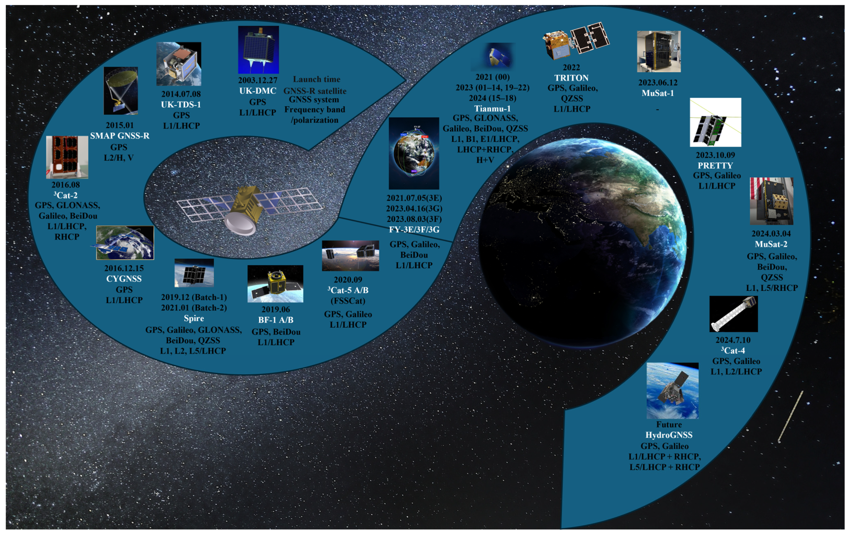
2. Current Status of Spaceborne GNSS-R Microsatellites

As an innovative remote sensing method, spaceborne GNSS-R technology has gained wide attention and applications in recent years. Using signals from navigation satellites and reflections from the Earth’s surface, spaceborne GNSS-R technology enables the monitoring of the oceans, the atmosphere, and terrestrial environments at a low cost with an elevated level of coverage and temporal resolution. Therefore, spaceborne GNSS-R technology has immense potential, especially in land, ocean, atmosphere, and cryosphere applications.

Early spaceborne GNSS-R missions focused on verifying the technology’s feasibility of this technology. In 2003, UK-DMC, the world’s first satellite carrying a GNSS-R receiver, received and processed the reflected signals from the Global Positioning System (GPS) L1 C/A code, thus verifying the feasibility of receiving GNSS-R signals from orbit and performing ocean remote sensing. Although its data is not publicly available, they provide a technical basis for subsequent missions [25]. This was followed in 2014 by the UK’s TechDemoSat-1 (TDS-1), which became another key advance in the field by measuring sea surface wind speed, sea ice thickness, and soil moisture and receiving GPS reflection signals. TDS-1’s successful collection of a large amount of data proved the potential of the GNSS-R technology for ocean and land remote sensing applications and laid a solid foundation for subsequent GNSS-R applications [26]. Subsequently, a significant GNSS-R mission, the Cyclone Global Navigation Satellite System (CYGNSS), launched by the National Aeronautics and Space Administration (NASA) in 2016, was a significant milestone in applying GNSS-R technology [27]. CYGNSS comprises eight microsatellites with high temporal resolution, which can observe tropical cyclones multiple times every few hours, providing valuable data support for extreme weather monitoring. In addition, the public disclosure of CYGNSS data provides scientists worldwide with rich research opportunities, extensively promoting the widespread application of GNSS-R technology. In 2018, the European Space Agency successfully launched ³Cat-5 A/B, consisting of two 6U cube satellites, as an early verification project of a small satellite federation system [28]. The Chinese BuFeng-1 A/B satellites were launched from a sea platform in 2019 to support measuring wind speeds at sea during typhoons and hurricanes. The instruments on each satellite include a direct-broadcast antenna, two 26-degree-tilted reflector high-gain antennas, a Global Navigation Satellite System-R receiver, and others. BuFeng-1 A/B not only collects Delay-Doppler Maps (DDMs) reflected by the Earth but also obtains the intermediate frequency (IF) raw data [29], marking China’s entry into the GNSS-R era. Since July 2021, China has launched FengYun-3E/3F/3G satellites to conduct global surface observations [30,31]. Many spaceborne missions have been launched in recent decades to exploit reflected GNSS signals; however, most provide DDMs of reflected GNSS signal power as their primary data product. The data products of complex waveforms of reflected signals can also be output using direct signal processing and open-loop model calculations of raw IF signals from multiple spaceborne missions [32]. The Spire satellite was also successfully launched in 2019. The Spire satellite constellation currently has over 100 3-unit cube satellites in low earth orbit at 450 to 600 km. Most of these satellites are dedicated to collecting GNSS-RO measurement data. The Spire GNSS-RO satellite’s instrument and antenna configuration enables it to receive earth-reflected signals from GNSS satellites at a ground-grazing angle (GA) [33], allow high-precision sea ice monitoring [34], and provide a new source of ionospheric data to mitigate the sparse availability of GNSS receivers over the ocean [35]. To map the distribution of inland water bodies, Zhang et al. [36] proposed jointly using the carrier phase and signal strength of the reflected signal to identify consistent reflections and applied this to GNSS-R measurements from the Spire and CYGNSS satellites. Since 2023, Muon Space has launched the MuSat-1 and MuSat-2 satellite missions, which can perform various Earth surface observations, such as soil moisture [37], wind speed at the ocean surface, surface water extent and inundation mapping, and sea ice characterization. MuSat-2 can also measure total electron content (TEC) using dual-frequency observations from multiple global navigation satellite system (GNSS) constellations [38]. The new generation GNSS-R receiver (NGRx) in the Rongowai mission can process multiple GNSS satellite signals simultaneously, with dual-polarization (Co-pol and Cross-pol) and dual-frequency (L1, L5) capabilities [39], significantly improving its potential for applications such as the remote sensing of the land surface, such as biomass estimation, soil moisture recovery, and flood monitoring [40].

Table 1 provides a brief introduction to GNSS missions and their application characteristics. Figure 1 shows the historical development of GNSS-R satellites, highlighting technological advances.

Figure 1. Development history of spaceborne GNSS-R satellites. Background image [41], UK DMC-1 [42], UK TDS-1 [43], CYGNSS [44], Soil Moisture Active Passive (SMAP) [45], PRETTY [46], Tianmu-1 [47], FY [48], ³Cat-2 [49], SPIRE [50], Bufeng-1 A/B [51], TRITON [52], FSSCat [53], ³Cat-4 [54], hydroGNSS [55], MuSat-1 [56], and MuSat-2 [57]. For more information, refer to UK DMC-1 [25,58], UK TDS-1 [26], SMAP [59], ³Cat-2 [60], CYGNSS [27], Spire [22,61], Bufeng-1 A/B [62], ³Cat-5A/B [28], FY-3E/G/F [30,31,63], TRITON [64], PRETTY [65], ³Cat-4 [66], and hydroGNSS [19].

Figure 1. Development history of spaceborne GNSS-R satellites. Background image [41], UK DMC-1 [42], UK TDS-1 [43], CYGNSS [44], Soil Moisture Active Passive (SMAP) [45], PRETTY [46], Tianmu-1 [47], FY [48], ³Cat-2 [49], SPIRE [50], Bufeng-1 A/B [51], TRITON [52], FSSCat [53], ³Cat-4 [54], hydroGNSS [55], MuSat-1 [56], and MuSat-2 [57]. For more information, refer to UK DMC-1 [25,58], UK TDS-1 [26], SMAP [59], ³Cat-2 [60], CYGNSS [27], Spire [22,61], Bufeng-1 A/B [62], ³Cat-5A/B [28], FY-3E/G/F [30,31,63], TRITON [64], PRETTY [65], ³Cat-4 [66], and hydroGNSS [19].

Table 1. Current major global navigation satellite system missions and their application characteristics.

Satellite	Sensor	Spatial Resolution	Temporal Resolution (Revisit Time)	Typical Applications	Data Coverage Ranges
UK-DMC-1 [25]	The GPS reflectometry payload	-	-	wind speed and wave [67].	Partial sea area
UK-TDS-1 [26]	A Space GPS receiver remote sensing instrument (SGR-ReSI)	-	More than 24 h	Ocean wind speed search, SM [68], monitoring of inland water bodies [69], water level [70], and sea ice [71].	-
CYGNSS [27]	Delay Doppler mapping instrument (DDMI)	25 km × 25 km	The average revisit time is about 7 h.	VWC [6], VOD [72], AGB, canopy height (CH) [7], water levels [73], river width and gradient [74], surface wind speed [75], red tide [76], SM [77], and flood monitoring [78].	North Bounding Coordinate: 40 degrees South Bounding Coordinate: −40 degrees West Bounding Coordinate: −180 degrees East Bounding Coordinate: 180 degrees
3Cat-2 [79]	The P(Y) and C/A reflectometer (PYCARO)	30 km	Revisit cycle less than 2 days	SM, AGB, altimetry, and surface wind speed [60].	-
SMAP GNSS-R [59]	The SMAP radar receiver	-	-	VWC [80], aboveground biomass (AGB) [59], F/T [81].	-
BuFeng-1 A/B [62]	One direct antenna, two 26-degree-tilted reflector high-gain antennas, and a GNSS-R receiver	-	-	-	From 53°S to 53°N
Spire [22,34,61,82,83]	A STRATOS dual-frequency GNSS receiver	-	-	The monitoring of inland water bodies [36], water levels [84], slope [85], SM [86], altimetry [33], and sea ice [34].	Batch-1: [−37,37] Batch-2: Global
FengYun-3E/3F/3G [30,31,87]	GNSS Radio Occultation Sounder II (GNOS II)	7 km × 0.5 km (on land)	approximately 1–2 days (at 36 km)	SM [87].	-
3Cat-5 A/B (FSSCat) [28]	Flexible Microwave PayLoad 2 (FMPL-2)	300 km to 40 m	daily	Soil moisture (SM), sea ice extent (SIE), concentration and thickness, and even wind speed [88].	Global
3Cat-4 [66]	Flexible Microwave PayLoad 1 (FMPL-1)	Sub kilometer	Global coverage the next day	-	-
PRETTY [65,89,90]	A passive GNSS-based reflectometer and dosimeter		Daily coverage of the polar region	Altimeter [91].	Global
TRITON (FORMOSAT-7R) [64,92,93]	The receiver is capable of handling the dispersed GPS, Galileo, and QZSS signals.	0.5. km to 25 km or 0.5 km to 40 km	-	surface wind speed [94].	-
HydroGNSS [19]	Delay Doppler mapping receiver (DDMR)	25 km	15 days	SM, AGB [95], F/T [19], flooded, or wetland [96].	Global
Tianmu-1 [23,97,98]	GNOS-M	Better than 25 km	Sampling approximately once every 1 s	surface wind speed [98].	-
MuSat-1 [56]	-	-	-	-	-
MuSat-2 [99]	A high-gain, beamforming GNSS-R payload	-	-	SM, Surface wind speed, the presence of vegetation or wetlands, and sea ice characteristics [38,57].	-

Table 1. Current major global navigation satellite system missions and their application characteristics.

Satellite	Sensor	Spatial Resolution	Temporal Resolution (Revisit Time)	Typical Applications	Data Coverage Ranges
UK-DMC-1 [25]	The GPS reflectometry payload	-	-	wind speed and wave [67].	Partial sea area
UK-TDS-1 [26]	A Space GPS receiver remote sensing instrument (SGR-ReSI)	-	More than 24 h	Ocean wind speed search, SM [68], monitoring of inland water bodies [69], water level [70], and sea ice [71].	-
CYGNSS [27]	Delay Doppler mapping instrument (DDMI)	25 km × 25 km	The average revisit time is about 7 h.	VWC [6], VOD [72], AGB, canopy height (CH) [7], water levels [73], river width and gradient [74], surface wind speed [75], red tide [76], SM [77], and flood monitoring [78].	North Bounding Coordinate: 40 degrees South Bounding Coordinate: −40 degrees West Bounding Coordinate: −180 degrees East Bounding Coordinate: 180 degrees
3Cat-2 [79]	The P(Y) and C/A reflectometer (PYCARO)	30 km	Revisit cycle less than 2 days	SM, AGB, altimetry, and surface wind speed [60].	-
SMAP GNSS-R [59]	The SMAP radar receiver	-	-	VWC [80], aboveground biomass (AGB) [59], F/T [81].	-
BuFeng-1 A/B [62]	One direct antenna, two 26-degree-tilted reflector high-gain antennas, and a GNSS-R receiver	-	-	-	From 53°S to 53°N
Spire [22,34,61,82,83]	A STRATOS dual-frequency GNSS receiver	-	-	The monitoring of inland water bodies [36], water levels [84], slope [85], SM [86], altimetry [33], and sea ice [34].	Batch-1: [−37,37] Batch-2: Global
FengYun-3E/3F/3G [30,31,87]	GNSS Radio Occultation Sounder II (GNOS II)	7 km × 0.5 km (on land)	approximately 1–2 days (at 36 km)	SM [87].	-
3Cat-5 A/B (FSSCat) [28]	Flexible Microwave PayLoad 2 (FMPL-2)	300 km to 40 m	daily	Soil moisture (SM), sea ice extent (SIE), concentration and thickness, and even wind speed [88].	Global
3Cat-4 [66]	Flexible Microwave PayLoad 1 (FMPL-1)	Sub kilometer	Global coverage the next day	-	-
PRETTY [65,89,90]	A passive GNSS-based reflectometer and dosimeter		Daily coverage of the polar region	Altimeter [91].	Global
TRITON (FORMOSAT-7R) [64,92,93]	The receiver is capable of handling the dispersed GPS, Galileo, and QZSS signals.	0.5. km to 25 km or 0.5 km to 40 km	-	surface wind speed [94].	-
HydroGNSS [19]	Delay Doppler mapping receiver (DDMR)	25 km	15 days	SM, AGB [95], F/T [19], flooded, or wetland [96].	Global
Tianmu-1 [23,97,98]	GNOS-M	Better than 25 km	Sampling approximately once every 1 s	surface wind speed [98].	-
MuSat-1 [56]	-	-	-	-	-
MuSat-2 [99]	A high-gain, beamforming GNSS-R payload	-	-	SM, Surface wind speed, the presence of vegetation or wetlands, and sea ice characteristics [38,57].	-

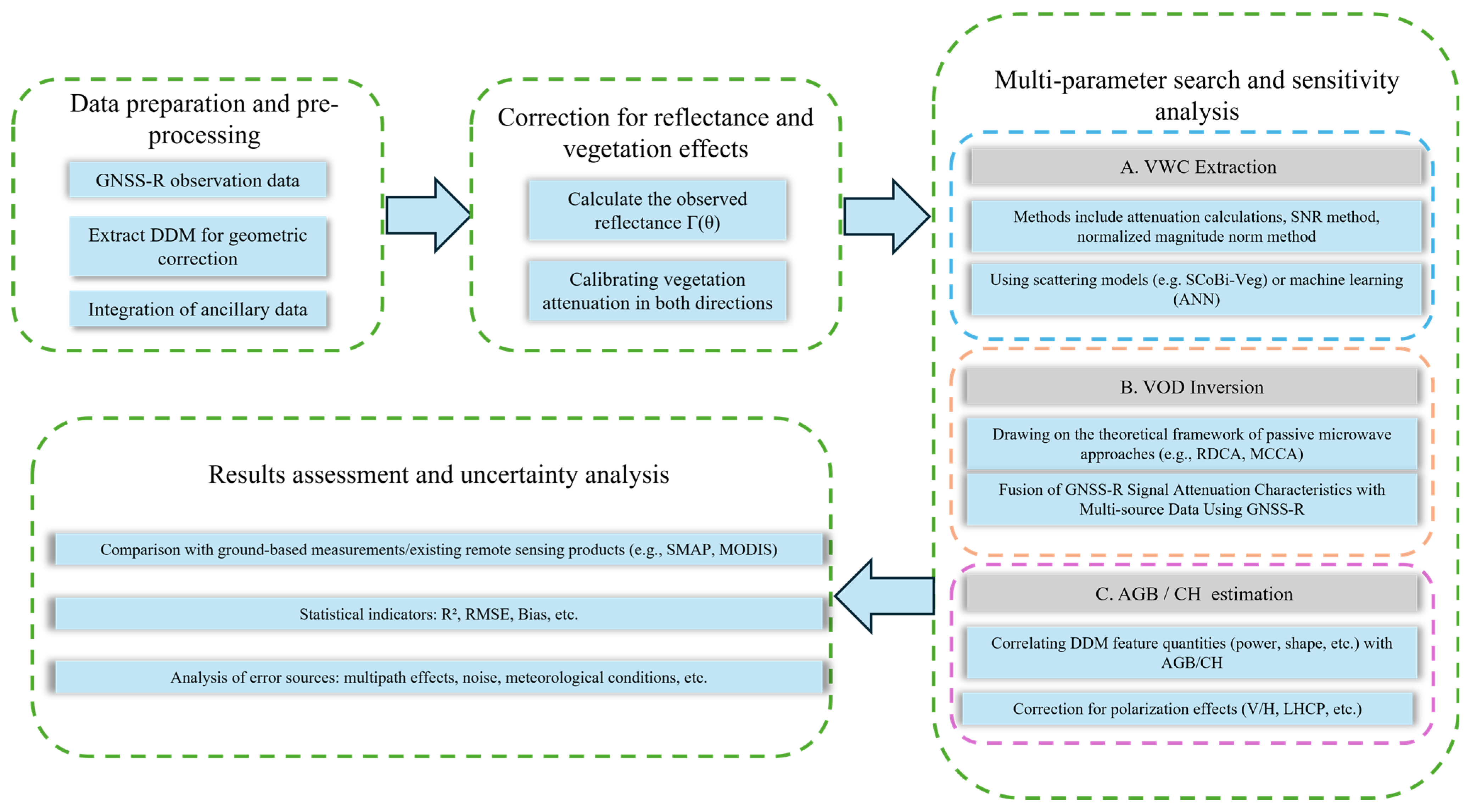
3. Vegetation Remote Sensing

3.1. Sensitivity Analysis of Spaceborne GNSS-R to Vegetation

Studying the sensitivity of spaceborne GNSS-R to vegetation is crucial for improving the accuracy and reliability of remote sensing data. Vegetation affects the reflection characteristics of GNSS-R signals. Therefore, through sensitivity analysis, we can better understand the impact of vegetation on signal attenuation, scattering, and other effects, thereby improving vegetation monitoring models and enhancing monitoring capabilities in areas such as soil moisture, ecological environments, and climate change.

The successful launch of the TDS-1 satellite in the UK in 2014 opened up new possibilities for monitoring land vegetation. Using data from the TDS-1 satellite, Camps et al. [100] found that GNSS-R technology shows strong vegetation sensitivity. When the normalized difference vegetation index (NDVI) value is low, the GNSS-R reflected signal shows stronger sensitivity to changes in soil moisture; as the NDVI increases, this sensitivity gradually weakens, but it still has a significant effect. Rodriguez-Alvarez et al. [80] analyzed the sensitivity of SMAP-reflectometry (SMAP-R) signals to VWC, which revealed that signal-to-noise ratio (SNR) decreases as VWC increases, and verified the feasibility of GNSS-R retrieve geophysical parameters. Through qualitative analysis, Yueh et al. [101] found that the effective reflectivity of CYGNSS decreased roughly linearly with NDVI-VWC. Their study laid the foundation for the coordinated use of reflectometry and radiometry data for multi-parameter retrieval and the development of consistent soil moisture products. The total power $P_r^S$ is the sum of the coherent and incoherent components, expressed as $P_c$ and $P_i$, respectively:

$$P_r^S=P_c+P_i$$

(1)

Their coherent reflection in the mirror direction can be expressed as [101]

$$P_c=\mathsf{\Gamma }(\theta ){\displaystyle \frac{{\lambda }^2{P}_t{G}_t{G}_r}{{(4\pi )}^2{(R_t+R_r)}^2}}$$

(2)

The bistatic radar equation can describe incoherent scattering [102]:

$$P_i={\displaystyle \frac{{\lambda }^2{P}_t{G}_t}{{\left(4\pi \right)}^3}}\int {\displaystyle \frac{G_r}{R_t^2{R}_r^2}}{\sigma }_s{\chi }^2(\tau ,f_D)dA$$

(3)

where $P_t{G}_t$ is the equivalent isotropic radiated power (EIRP) of the GPS, inferred from direct measurements of CYGNSS; $G_r$ is the antenna gain pointing toward the specular point; $R_t$ is the distance between the GPS transmitter and the specular point; $R_r$ is the distance between the CYGNSS receiver and the specular point; $\mathsf{\Gamma }(\theta )$ is the coherent reflectivity at the angle of incidence $(\theta )$; $\lambda$ is the GPS wavelength; ${\sigma }_s$ is the incoherent normalized radar cross section for rough surfaces and vegetation; and ${\chi }^2$ is the Woodward ambiguity function (WAF).

Surface reflectivity is affected by multiple factors, such as soil, vegetation, and topography. In areas with sparse vegetation and flat terrain, the influence of the soil dielectric constant and soil moisture on reflectivity is more significant; vegetation attenuation plays a key role in areas with dense vegetation. At the same time, surface roughness affects reflectivity through diffuse scattering processes, but for satellite observations, the impact of large-scale terrain is usually more significant than small-scale roughness.

Satellite systems using spaceborne GNSS-R technology mainly receive GNSS signals and are widely used in vegetation monitoring. Vegetation monitoring based on spaceborne GNSS-R data has achieved remarkable results in North America, Europe, Asia, and other regions. GNSS reflection signals contain various characteristics information, providing key data for vegetation and surface parameter estimation. However, current applications are relatively focused on GPS signals, and the potential development of other global navigation satellite systems (such as GLONASS, Galileo, BeiDou, and others) must be explored in depth. In general, applying spaceborne GNSS-R technology in different regions provides a new means for vegetation remote sensing. Still, the model needs further improvements to correct vegetation absorption and scattering effects. In addition, future development directions should include expansion to other GNSS signals to achieve more comprehensive and accurate vegetation and soil moisture monitoring capabilities.

3.2. Vegetation Water Content

VWC is a key factor affecting vegetation growth, activity, and biomass and plays a vital role in ecosystems’ water cycle and biogeochemical processes. Traditional VWC monitoring methods mainly rely on on-site measurements, which are limited by the spatial and temporal scales of the data [103]. Remote sensing techniques (including optical and microwave remote sensing) have become an alternative. Optical remote sensing has high spatial resolution but is susceptible to cloud cover [104], while microwave remote sensing has a strong penetration ability and can obtain data under cloud cover. Still, its resolution is low and is affected by ground roughness and soil moisture [105]. The GNSS-R passive remote sensing method has gradually become a new monitoring method due to its sensitivity to VWC in recent years. By analyzing the ground reflection characteristics such as signal strength, the polarization ratio, and the Doppler effect, GNSS-R signals can provide long-term time series data of vegetation water changes. Compared with traditional remote sensing methods, GNSS-R technology has the unique advantage of avoiding clouds and shadows to provide more stable and continuous monitoring data. Therefore, applying GNSS-R technology to monitor VWC has excellent potential and research value.

Small et al. [106] are the first to show a qualitative consistency between reflections recorded by GPS receivers and vegetation growth. Rodriguez-Alvarez et al. [107] studied the GNSS-R technique for estimating VWC by measuring and analyzing the received power of the GPS signal in the open sky and under the vegetation layer, calculating the attenuation caused by vegetation and inferring information about VWC. There is good consistency. The power received by the instrument is used to calculate the attenuation caused by vegetation, and the formula is as follows:

$${\displaystyle \frac{P_A}{P_B}}={\displaystyle \frac{{|L\cdot E_A|}^2}{{\left|E_B\right|}^2}}={\displaystyle \frac{{\left|L\right|}^2\cdot {|E_{0i}\cdot e^{j{\varphi }_A}|}^2}{{|E_{0i}\cdot e^{j{\varphi }_B}|}^2}}={\left|L\right|}^2=L^2$$

(4)

where $P_A$ and $P_B$ is the powers received by instruments $A$ and $B$, respectively, $L$ is the attenuation caused by vegetation, $E_{0i}$ is the amplitude of the incident electric field (the amplitude is the same for both instruments because the attenuation has already been taken into account by using the factor $L$), and ${\varphi }_A$ and ${\varphi }_B$ are the phases of the incident electric field for each instrument.

Chew et al. [108] proposed that the fundamental change in GPS (signal-to-noise ratio) SNR data is related to the vegetation canopy. Wan et al. [109] confirmed that there is consistency between SNR data and VWC and that temperature minimally affects the SNR data. Eroglu et al. [110] used the scattering model SCoBi-Veg to accurately characterize the vegetation effect and found that the specular component of the reflected signal dominates at moderate surface roughness, and there is a significant correlation between VWC and the cross-polarized reflected signal. Guerriero et al. [111] considered the propagation and scattering of left and right circularly polarized signals. The results showed that right-polarized measurements are mainly affected by coherent signal attenuation, while left-polarized measurements are almost entirely affected by incoherent volumetric scattering. Chen et al. [6] found a linear relationship between CYGNSS reflectivity and soil moisture using the tau-omega model, where the slope (A) and intercept (B) are related to vegetation characteristics. The use of artificial neural network (ANN) models for VWC retrieval is consistent, but the technology for fusing multiple remote sensing parameters is still immature. Therefore, Zhang et al. [112] constructed a GNSS-R VWC retrieval model that integrates key information such as the bistatic radar cross section (BRCS), the effective scattering area, CYGNSS variables, and surface auxiliary parameters and tested the performance of different models. The results show that the root mean square error (RMSE) of the random forest (RF) and bagging tree (BT) models is 0.50 kg/m², which is better than other models. Asgarimehr et al. [113] studied the diurnal cycle of VWC and its response to water stress in the Amazon region. The results showed significant differences in the morning and evening VWC during the wet and dry seasons. Emphasized that GNSS-R can achieve high-frequency monitoring of tropical rainforests.

GNSS-R technology shows excellent potential in monitoring VWC. Still, it faces some challenges, such as the effects of vegetation type, climate, and topography on the reflected signals; the multipath effect of the signals; and the interference of soil moisture. Future research should optimize models and algorithms and combine multi-source remote sensing data and ML techniques to improve monitoring accuracy and adaptability and enhance GNSS-R technology’s ability to be applied globally.

3.3. Vegetation Optical Depth

VOD is a key indicator of plant water status. It is closely related to vegetation biomass, soil moisture, and the various physiological characteristics of plants, such as leaf water potential and overall health.

Remote sensing technology is vital in studying plant water and related processes. The attenuation effect of water inside plants on microwave signals and the extinction of microwave radiation in the plant canopy can be used to calculate the VOD. Chaubell et al. [114] use the regularized dual-channel algorithm (RDCA) to effectively improve the retrieval accuracy of soil moisture and vegetation optical depth (VOD) by combining H and V polarization brightness temperature measurements, and the VOD retrieval results are consistent with the trend of SMOS products. Hu et al. [115] use the multi-channel collaborative algorithm (MCCA), which is based on a two-component model, to link microwave brightness temperature observations under different frequencies and polarization conditions in a multi-channel environment. The formula is as follows:

$$T{B}_{ch}^{measured}=V_{ch}^e+V_{ch}^t•e_{ch}^s$$

(5)

The subscript $ch$ represents the different channels and is used below to denote polarization $(P)$, the angle of incidence $(\theta )$, and frequency $(f)$; the superscript s denotes the rough soil surface; $T{B}_{ch}^{measured}$ is the total brightness temperature measured at channel $ch$; $e_{ch}^s$ denotes the emissivity from the rough soil surface, which is a function of the soil dielectric constant ${ϵ}_{ch}^s$ and the surface roughness; $V_{ch}^e$ is the vegetation emission term; and $V_{ch}^t$ is the vegetation transmission term.

The global soil moisture and frequency- and polarization-dependent VOD products developed from AMSR-E/2 microwave remote sensing data have good global applicability. Liu et al. [116] proposed that global C-band data based on Advanced Scatterometer (ASCAT) active microwave data use a water cloud model (WCM) and introduced a multi-temporal (MT) retrieval method to stabilize the retrieval parameters to simultaneously retrieve VOD and vegetation scattering parameters (ω).

Microwave remote sensing can extract VOD by measuring the attenuation of microwave signals from the vegetation, which reflects the water status of plants. However, it has many limitations in monitoring soil moisture and vegetation biomass, such as the fixed transit time of sun-synchronous satellites, which limits the capture of diurnal changes due to low spatial resolution and difficulty distinguishing the multiple process contributions to VOD. Recent studies have shown that the attenuation effect of GNSS signals can also be used to monitor VOD, providing continuous observation data with higher temporal resolution. The GNSS signal is also affected by moisture when passing through the vegetation canopy, so changes in the GNSS signal can be used to estimate VOD. The advantage of this method is that it can provide data at a higher frequency at the sub-hourly level, which helps study the diurnal cycle of VOD and its relationship with plant water dynamics.

Santi et al. [72] validated the potential of GNSS-R data in observing vegetation parameters and attempted to combine CYGNSS and ML to estimate forest biomass. Xu et al. [117] proposed a new method for retrieving VOD using the effective reflectivity of CYGNSS and developed a physical model based on a dielectric constant model. The results show that the VOD retrieved by CYGNSS highly correlates with SMAP data in agricultural areas. However, the model needs to be further optimized to consider the effect of biomass on reflectivity. Pierdicca et al. [20] explored GNSS-R and its application in the detection of vegetation dynamics. The study utilized satellite data and found that GNSS-R reflectivity was negatively correlated with the sensitivity of VOD. The model further verified that GNSS-R reflectivity is significantly affected by vegetation absorption and scattering. Bu et al. [118] combine the extreme random tree (ET) model with retrieve VOD and integrate BRCS with the effective scattering area and surface parameters, Their approach achieves superior accuracy compared to adaptive boosting (AdaBoost), the support vector machine (SVM), and gradient boosting decision trees (GBDTs). The RMSE is improved by 178.12%, 67.87%, and 85.26%, and the MAPE is improved by 87.50%, 80.00%, and 92.31%, making it suitable for high-precision VOD retrieval. Yao et al. [119] utilized the GNSS signal attenuation characteristics to monitor the diurnal and seasonal variations in VOD in temperate broadleaf forests on a sub-hourly basis, revealing significant correlations with leaf water potential (R² = 0.68) and daily maximum VOD.

3.4. Forest Aboveground Biomass and Canopy Height

AGB and CH are key indicators of forest health, carbon storage, and ecological functioning. AGB represents the total mass of all living plants in the forest and is an essential basis for assessing the carbon sequestration capacity of forests and the role of climate regulation. CH reflects the vertical structure of the forest and affects light distribution and ecological diversity.

GNSS-R technology has obvious advantages over traditional methods in retrieving AGB and CH. Conventional methods, such as empirical modeling based on the field tree height and the diameter at breast height [120], are highly accurate but costly and time-consuming [121], and the accuracy may be reduced in large-scale applications. While more accurate, remote sensing technologies such as LiDAR [122] and synthetic aperture radar (SAR) are limited by high costs [123]. In contrast, GNSS-R technology can penetrate clouds and vegetation by receiving satellite reflection signals; has global coverage, low cost, low power consumption; and is not limited by weather and terrain.

Carreno-Luengo et al. [124] proposed to analyze the relationship between multiple observable measurements from DDMs and AGB by finding that the trailing edge width (TE) and reflectivity (Γ) are sensitive to forest AGB, and this sensitivity depends on elevation angles, with the optimal elevation angle varying depending on the forest type with elevation angles varying depending on forest type. In rainforests, the trailing edge width (TE) at low elevation angles and the reflectivity (Γ) at moderate elevation angles can maintain sensitivity to AGB up to 350 tons per hectare without saturation. Γ outperforms TE at low AGB. By combining CYGNSS observations, SMAP soil moisture data, and localization information, Chen et al. [7] proposed an improved retrieval method for AGB and CH using an artificial neural network (ANN), which outperformed the traditional method. Different satellite GNSS-R receiving antenna polarization methods (SMAP: V/H linear polarization; TDS-1, CYGNSS: left-handed circular polarization (LHCP)) significantly affects vegetation monitoring. Traditional GNSS-R retrievals mostly use only DDM peaks and ignore latent information; therefore, Pilikos et al. [125] proposed a novel DL retrieval model for biomass estimation using the full DDM of surface reflectivity, which was shown to be more superior on global and regional scales, with less biomass target error, providing more information while enhancing the model’s robustness to the robustness of the reflectivity signal from the vegetation. However, the complex process of calibrating the retrieval model remains a problem.

GNSS-R data are susceptible to forest parameters and show good potential for forest biomass retrieval. In the future, more reliable ground truth data and updated reference maps need to be introduced to further evaluate its ability in terms of spatial resolution. In addition, auxiliary retrieval combined with other surface parameters (such as soil moisture) may improve the retrieval accuracy. At the same time, exploring other information in DDM data is possible.

However, the research on GNSS-R in terrestrial remote sensing applications is still in its infancy, and most of it is currently focused on sensitivity analyses of vegetation parameters, lacking an in-depth understanding of the physical mechanisms. The retrieval accuracy is expected to improve with ML, especially neural network methods. Current GNSS-R satellites still have limitations, such as coverage and signal variability, and further research is urgently needed. In the future, as datasets and tasks improve, techniques based on complex retrieval algorithms will help improve the retrieval quality of biogeophysical parameters such as forest biomass and promote the practical application of this technology in vegetation remote sensing.

Figure 2 demonstrates the four stages of the vegetation parameter extraction process based on spaceborne GNSS-R data: data preprocessing, reflectivity and vegetation effect correction, multi-parameter extraction and sensitivity analysis, and result evaluation. VWC, VOD, and AGB were extracted through the integrated processing of GNSS-R signals and auxiliary data. Finally, the results are evaluated using ground observation data and statistical indicators to provide a reference for applying GNSS-R technology in vegetation monitoring.

To understand the current application status and research progress of spaceborne GNSS-R technology in vegetation parameter monitoring, we have summarized the relevant work, as shown in

Table 2. Current status and summary of spaceborne GNSS-R technology vegetation parameter monitoring-related work.

Vegetation Parameters	Literature	Satellites	Spatial Coverage	GNSS-R Observables	Auxiliary Data	Reference Data	Retrieval Models	Retrieval Accuracy
AGB and CH	[7]	CYGNSS	Quasi-global	Traditional Reflectivity (Γsurrface) and Correction Reflectivity (ΓLR (${\mathit{\epsilon }}_S$, θi)/${\sigma }_0^{coh}$)	AGB map derived from LUCID and ICESat/GLAS CHt	SMAP soil moisture	ANN	The RMSE was reduced by 11.63% and R was improved by 5.26% using the AGB method, while the RMSE was reduced by 12.59% and R was improved by 5.06% using the CH method.
	[20]	CYGNSS	Manaus, Algorta, Fairbanks, and Asuncion	Reflectivity, SNR, and DDM peak	SMAP VOD	MODIS NDVI	ANN	RMSE = 0.1 and R = 0.924
	[111]	Ground-Based	Poplar forests of four different biomasses in Tuscany, Italy	GNSS signal power and polarization	Ground truth vegetation biomass, tree density, LAI, and SMC	Vegetation height	ANN	The RMSE is about 10 tons/hectare, and the R is close to 1.
	[124]	CYGNSS	Congo and Amazon rainforests	Reflected delay waveforms, trailing edge width (TE), reflectivity (Γ)	land Elevation Satellite (ICESat-1)/Geoscience Laser Altimeter System (GLAS) AGB	SMAP-derived VOD, PI, and SMC	linear regressions”	The sensitivities between the trailing edge AGB and the roughness parameter Γ are 350 t/ha and 250 t/ha, respectively.
	[125]	CYGNSS	South America, Central Africa	DDMs, equivalent surface reflectivity Γ, and SNR	ESA CCI biomass map	-	neural networks	R = 0.962 and RMSE = 25.65 t/ha.
VOD	[117]	CYGNSS	Tropical forest regions, agricultural land, and the global scale	Reflectivity	SMAP soil moisture data	SMAP VOD NDVI VOD	Semi-empirical forward model	The VOD data inverted by CYGNSS are more consistent with SMAP data in agricultural areas and lower in forested areas.
VWC	[6]	CYGNSS	Quasi-global	The coefficient and intercept feature derived from the tau-omega model	SMAP VWC	SMAP SM, the land cover, and NDVI derived from MODIS	Linear model and ANN	CYGNSS VWC retrieval (ANN: R = 0.940 and RMSE = 1.392 kg/m2) outperforms the linear model.
	[113]	CYGNSS	Amazon rainforest	Reflectivity	SMAP soil moisture	AmeriFlux PE-QFR site data	Linear model	GNSS-R VWC are consistent with SMAP-derived VWC

.

4. Retrieval of Physical Parameters of Inland Water Bodies

4.1. Detection of Inland Water Bodies

Inland surface water bodies (rivers, lakes, reservoirs, wetlands, and others) are essential components of the Earth system, affecting the hydrological cycle, energy exchange, and carbon cycle. They are significant to human society and the climate, requiring high spatial and temporal resolution to monitor surface water dynamics and remote sensing technology. Optical, microwave radar, and radiation are widely used to map the surface water distribution [126,127]; optical images have a high spatial resolution but are susceptible to weather and vegetation [128], and microwave observations are highly resistant to interference but have low time resolution. GNSS-R provides a new solution, with the advantage of being weather-independent and light-independent, enabling the continuous monitoring of water bodies under more weather conditions. By analyzing satellite signals reflected from the water surface, GNSS-R can accurately detect the existence of water bodies and their dynamics, especially during floods or other extreme weather events. The application of this technology increases the reliability and frequency of monitoring, making water resource management and disaster prevention more efficient and timelier.

Since coherent reflection and incoherent scattering are different physical effects closely related to the scene and sensor characteristics, identifying the dominance of coherent or incoherent effects in CYGNSS measurements is crucial to support surface studies. For this reason, Al-Khaldi et al. [129] analyze the distribution of the power across the DDM using a Power Ratio (PR) to detect coherence. The algorithm can efficiently mark coherent regions, especially water bodies or exceptionally smooth surface areas such as deserts. To solve the problem of unreasonable threshold selection, Wang et al. [130] proposed an algorithm based on a SVM to detect coherent reflections. The detection accuracy of this algorithm is 98.66%, superior to other detection methods based on thresholding and logistic regression. However, the incoherent scattering component in the reflection signal often leads to cycle slips in conventional open-loop (OL) tracking methods, which in turn causes meter-level errors. Therefore, Wang et al. [131] proposed a synchronized cycle slip and noise filtering (SCANF) algorithm that combines signal amplitude measurements and is capable of efficient real-time operation. Experimental results show that the algorithm can achieve accurate centimeter-level sea surface height anomaly (SSHA) retrieval in practical applications. However, the algorithm still needs to be improved, especially in optimizing the noise model, handling ionospheric/tropospheric multipath fluctuations, and calibrating the SNR measurement according to the antenna gain pattern, for which an adaptive hybrid tracking (AHT) algorithm is proposed by Wang and Morton [132]. Utilizing a Doppler model to assist adaptive closed-loop (ACL) tracking effectively integrates the mechanisms typically employed in MS-OL and CL carrier phase tracking systems with good robustness.

The primary collection of raw IF data from multiple spaceborne missions provide a valuable opportunity to explore the potential of GNSS-R technology in advanced geophysical applications and future missions. Therefore, Li et al. [32] generated complex waveform data products that included amplitude and carrier phase information by processing raw GNSS reflection signal data collected from multiple space missions. The existence of water bodies can be effectively identified by analyzing the phase information and amplitude of the reflected signal. Using these complex waveform data, new applications of GNSS-R technology in future spaceborne missions can be further explored. Mei et al. [133] used CYGNSS IF data to verify the effectiveness of the method in combination with Sentinel-2 NDWI and Sentinel-1 SAR images. The results show that the comprehensive method has an accuracy of 80–91%, which is better than the single feature method, and has a high time resolution of 20Hz, which is suitable for the detection of small-scale water bodies. In [36,134], they developed a method that integrates the carrier phase and signal strength to detect coherent reflections, enabling effective monitoring of inland water bodies. The results indicate that compared to observations from global surface water resource managers, Spire data have a 90% difference in water boundaries of less than 0.73 km, with an average difference of 0.28 km; the 90% difference in CYGNSS data is less than 0.43 km, with an average difference of 0.18 km. This indicates that the method has high accuracy in drawing surface water maps. In [135,136], they proposed a new CYGNSS data product based on raw IF data that includes several well-established signal coherence detectors, including the power ratio P_ratio, the complex zero-Doppler delay waveform, total entropy E_full, and a new fast entropy detector E_fast, which can effectively capture surface features. Fast entropy achieves performance comparable to full entropy at low computational costs and is particularly effective in detecting small bodies of water. Different researchers have proposed different GNSS-R coherence detection methods. Since these methods are applied in various scenarios and quantified differently, comparing their advantages and disadvantages is difficult. Therefore, Loria et al. [137] conducted a unified comparison of various GNSS-R coherence detection methods. The results show that shape-based algorithms (such as first-order PR and entropy) have good detection performance and do not require accurate DDM power calibration. The choice of algorithm should be optimized for specific application scenarios, particularly for real-time in-orbit processing and post-processing applications, which have different advantages. Traditional satellite remote sensing systems cannot reliably detect biomass-dense inland waters. Therefore, Carreno-Luengo et al. [138] discussed the ability of the CYGNSS mission to detect small water bodies under high-density vegetation in complex and heterogeneous scenes such as tropical rainforests through the power ratio and reflectivity feature. Despite the influence of the intermediate vegetation cover, GPS signals can still be coherently reflected from surface water bodies, detect and image small water bodies with lush vegetation, and even surface water with low water levels. Du et al. [139] proposed a new spaceborne processing strategy that coherently combines the reflected (GPS) III level 1 (L1) C/A and L1C signals, which can significantly improve the SNR using additional signal components. The auto-correlation function of the combined signal is defined as follows:

$$\begin{array}{c}{R}_{\mathrm{com}}(\tau )={\displaystyle \frac{1}{2}}{R}_{\mathrm{L}1\mathrm{C}/\mathrm{A}}(\tau )+{\displaystyle \frac{1}{2}}{R}_{\mathrm{L}1\mathrm{C}}(\tau )\\ =\left\{\begin{array}{cc}1-{\displaystyle \frac{2\left|\tau \right|}{T_{\mathrm{chip}}}},& |\tau |<{\displaystyle \frac{T_{\mathrm{chip}}}{2}}\\ 0,& \mathrm{else}.\end{array}\right.\hfill \end{array}$$

(6)

where $T_{\mathrm{chip}}$ is the duration of the code chip and $\tau$ is the code delay.

The combined signal’s auto-correlation function is narrower, further improving geophysical applications’ spatial resolution and performance. The next generation of GNSS-R payloads will be able to process multiple types of reflected GNSS signals, improving sensing capabilities and thus expanding potential applications. Kossieris et al. [140] used CYGNSS data combined with unsupervised learning algorithms for inland water detection. They used clustering methods such as K-means, agglomerate, and density-based spatial clustering of applications with noise (DBSCAN) to automatically identify water bodies. The research results show that the K-means algorithm performs the best in accuracy, reaching 93.5%; the DBSCAN algorithm achieved the highest recall rate of 83.1%. The polarized GNSS-R system improves the accuracy of remote sensing through additional polarization channels [141]. Peng et al. [142] analyzed the impact of right-handed polarized signals on the GNSS-R water detection algorithm and proposed that dual-polarized GNSS-R data can significantly improve water detection capability and reduce the reliance on auxiliary data.

Figure 3 shows the monitoring process of inland water bodies based on CYGNSS signals, including data input, direct and reflected signal preprocessing, signal phase correction, and weighted combination to generate a combined signal with an enhanced SNR. Finally, monitoring effectiveness is validated through waveform analysis and resolution enhancement.

The sensitivity of CYGNSS to inland water bodies is widely recognized, but relying solely on CYGNSS for water body detection is uncertain, which poses a challenge to large-scale accurate detection. Therefore, Chen and Yan [143] proposed a contextual feature refinement method (CFRT) that combines multi-source data to detect inland water bodies worldwide. This method accurately predicts water bodies using CYGNSS reflection signals, vegetation parameters, terrain data, and geographical location information. This method significantly reduces the error (RMSE = 7.15%) compared to traditional DL models and improves the spatial consistency of water body detection (intersection over union = 0.778). To monitor inundation in areas with dense vegetation and cloud cover [144], a water body mask based on a random walk algorithm was developed to monitor seasonal dynamics in tropical regions. Combining the high temporal resolution of CYGNSS data with the penetrating power of L-band microwave and computer vision generates a monthly water mask with a spatial resolution of 0.01° (about 1 km). The product shows more significant seasonal water body changes. Peng et al. [96] extended the water body monitoring algorithm to dual-frequency and dual-polarization data by utilizing a random forest classifier and integrating coherence metrics from low-rate power signals (PSR and reflectivity) with high-rate complex signals (coherence coefficient and normalized amplitude); the classification accuracy exceeded 90%.

Although GNSS-R technology shows excellent potential in inland water monitoring, it still faces many challenges. The primary problem is the impact of complex heterogeneous surface environments on GNSS-R signals, especially in areas with high-density vegetation cover, such as tropical rainforests. Dense vegetation attenuates and scatters GNSS signals, reducing the coherence of the reflected signal from the water body and making it difficult to identify the water body. In addition, temporal and spatial changes in the vegetation type, vegetation cover, and biomass can also affect the consistency and reliability of GNSS-R observations. Therefore, there is an urgent need to develop advanced algorithms that can effectively deal with the impact of vegetation and extract water body information. At the same time, the fusion of multi-source remote sensing data (such as optical, radar, and radiometer data) and the use of ML and other techniques to combine multidimensional feature information are expected to further enhance the ability to detect and map water bodies in complex environments and expand the scope of GNSS-R applications. Future research needs to focus on overcoming these key scientific issues and tapping the potential of GNSS-R in global land hydrology research.

4.2. Water Level

Monitoring the water level of lakes is an integral part of hydrological research. Standard methods include hydrological station measurements and satellite altimeters. Hydrological stations are sparsely distributed and difficult to establish in harsh environments, while satellite altimeters provide higher temporal and spatial resolution. However, current satellite altimetry missions can only monitor water volume changes in 15% of the world’s inland water bodies due to resolution limitations. GNSS-R technology can be regarded as a radar altimeter, using GNSS satellites as the emission source. Still, it has mainly focused on sea level in the past, and little research has been performed on inland lake water levels.

GNSS-R technology measures water level by analyzing the delay between the direct and reflected signals of GNSS satellites. The existing height measurement techniques can be divided into code delay-based height measurement and carrier phase-based height measurement. Code delay height measurement relies on changes in ranging codes to calculate height, which requires less signal coherence and stronger adaptability. However, due to the chip width of the GNSS signal and the limitations of the reflected signal strength, its accuracy is relatively low [145]. Phase-based altimetry can achieve centimeter-level measurement accuracy [146], but it has high requirements for signal coherence and is susceptible to interference when sea surface roughness increases [147]. Semmling et al. [148] proposed that the spectral search method can tolerate sea surface standard deviations (≤30 cm) and is suitable for sea conditions with high wave heights. Cardellach et al. [147] first used a space platform to realize carrier phase sea surface altimetry. The altimetry results show that the accuracy of the carrier phase-based altimeter (CaPA) technology is in the sub-decimeter range, with a system accuracy of 3.0 cm (median) at 20 Hz and up to 16 cm.

Xu et al. [70] studied the feasibility of using TDS-1 global navigation satellite system reflection data to estimate global lake water levels. However, the data quality and accuracy still need to be improved. Since the GNSS signal reflected from water surfaces has a significantly different received power than land, this difference can be used to generate relevant maps. Loria et al. [149] used a complete forward scattering model approach to assess the accuracy of wetland extent retrieval algorithms, and the results showed that scattering from outside the first Fresnel zone and instrument effects can affect the accuracy. Factors such as surface shape, vegetation attenuation, and surface roughness further complicate the measurement, and adequate characterization of these other factors is required to accurately estimate these variables. To assess the performance of the large number of DDMs recorded by the CYGNSS satellites in estimating inland water levels, Zhang and Morton [5] modeled the range delay of the reflected signal as follows:

$${\rho }_m={\rho }_m^{\mathrm{GEOM}}+{\rho }_m^{\mathrm{IONO}}+{\rho }_m^{\mathrm{TROPO}}+{\rho }_m^{\mathrm{SET}}.$$

(7)

where ${\rho }_m^{\mathrm{GEOM}}$ indicates the geometric distance between the GPS transmitter, SP, and CYGNSS receiver; ${\rho }_m^{\mathrm{IONO}}$ indicates the ionospheric delay of direct and reflected signals; ${\rho }_m^{\mathrm{TROPO}}$ indicates the tropospheric delay of reflected signals; and ${\rho }_m^{\mathrm{SET}}$ indicates solid Earth tide.

The water level is calculated with the position relationship between the satellite and the water surface. The overall results show that the water level estimation of CYGNSS data has a deviation of about 2 m compared to RA data, RMSE of 3.1 m, and an unbiased root mean square difference (ubRMSD) of 2.4 m. This study shows that GNSS-based reflection altimetry can effectively monitor reservoirs and flood events with drastic changes in the water level. Brendle et al. [150] proposed a method to estimate the water level by tracking the change in reflectivity near the reservoir boundary. CYGNSS data can estimate the reservoir water level within one day, and the correlation with the on-site measured data can be as high as 86%. For periods when the reservoir water level changes significantly, this method effectively captures the dynamic changes in the water level. Yanez et al. [84] used Spire’s grazing GNSS-R data to compare and analyze the radar altimetry data from the Sentinel-3 satellite, which showed that combining the two techniques could achieve an estimated water level accuracy of within 6 cm. In addition, GNSS-R data can also independently verify the accuracy of radar altimetry data, especially in areas where ground monitoring is lacking. This provides basic research for future multi-technology-integrated hydrological products. Ma et al. [73] proposed a method for rapidly estimating the water level and depth of inland water bodies by combining CYGNSS L1 data and digital terrain models (DTMs). The results showed that the method was highly correlated in flood monitoring (average R is 0.98) and also showed some consistency in monitoring long-term changes in lakes and reservoirs, which can be used to monitor sudden floods and long-term changes). GNSS-R phase altimetry measurements have a constant but unknown offset and may be affected by residual atmospheric errors after model correction. Therefore, Wang et al. [151] improves the accuracy of surface height measurements through cross-adjustment. In the case of Lake Ladoga, the accuracy after cross-adjustment is very high, with a root mean square difference (RMSD) of about 3 cm.

Figure 4 shows the process of water level estimation based on GNSS-R data, including data input (delay-Doppler diagram, reflection point position, and others), pre-processing (data quality filtering and temporal and spatial consistency), reflection point and delay calculation, level modeling, and a systematic framework for validation and spatiotemporal analysis using both measured and satellite data.

Table 3. Current status and summary of related work on water level estimation using spaceborne GNSS-R.

Source	Satellites	Spatial Coverage (Resolution)	GNSS-R Observables	Reference Data	Retrieval Models	Retrieval Accuracy
[5]	CYGNSS	Five lakes	Reflection signal delay and SNR	DAHITI and Hydroweb	-	The accuracy of inland water surface elevation can reach 2–3 m.
[70]	TDS-1	500 square kilometers	DDMs	CryoSat-2 data and Hydroweb data	-	Overall R2 greater than 0.95.
[73]	CYGNSS	three floods, three lakes, and two reservoirs	Surface reflectivity	ICESat-2, GEDI, DAHITI, and Hydroweb	A water level retrieval method based on CYGNSS and the digital terrain model (DTM)	The water level recovery method combining CYGNSS and DTM data is effective.
[84]	Spire	Great Lakes of North America	Raw IF data	NOAA CO-OPS network height data and mean lake surface (MLS)	-	The use of GNSS radio measurements to supplement RA observations has advantages.
[150]	CYGNSS	Okeechobee Lake, Bull Shoals Lake, and Mead Lake	Normalized BISTATIC radar cross section (NBRCS) and surface reflectivity	In situ water level data and planet satellite imagery from NASA SEDAC	Empirical linear models	For reasonable performance, at least 15 2 Hz measurements per day are required in the “edge area”.
[151]	Spire	Lake Ladoga	carrier phases, and SNR	ICESat-2 altimetry measurements, and the geoid model EGM2008	least-squares adjustment techniques	root-mean-square (RMS) = 3 cm

summarizes the status and related research work on water level estimation using spatial GNSS-R technology

4.3. River Width and Slope

A river’s slope and width are two crucial parameters in hydrological research. They are significant for estimating a river’s flow rate and velocity. The river’s slope is affected by terrain and weather. Traditional river slope data mostly come from terrain models and elevation measurements [126], which have certain timeliness and accuracy issues. River width is an essential input parameter for hydrological models. It is the basis for predicting hydrological phenomena such as floods and sediment transport and is closely related to changes in flow. Data on river width is usually obtained through long-term satellite observations. Images provided by satellites such as Shuttle Radar Topography Mission (SRTM) [152] and Landsat [153] can reflect the river’s range at a specific point in time. However, these data cannot capture the dynamic changes in the river promptly. The current GNSS-R method has the potential to provide large-scale data with high temporal resolution that can be used as the input for estimation algorithms.

Warnock and Ruf [154] showed a high correlation between river width measured from GNSS-R signals and river flow, and this technique can be used to estimate river flow. Wang and Morton [155] confirmed the potential of GNSS-R carrier phase measurements to estimate river surface slope as follows:

$$H=H_{\mathrm{Ref}}-{\displaystyle \frac{\delta {\mathsf{\Phi }}_s}{2\sin \theta }}$$

(8)

where $H_{\mathrm{Re}\mathrm{f}}$ is the reference height of the river surface, $\theta$ is the elevation angle at SP, and $\delta {\mathsf{\Phi }}_s$ is the estimated excess phase of the reflected signal due to changes in the height of the reflecting surface.

The gradient of multiple river sections was obtained through OL tracking of the carrier phase of the reflected signal and search, and a novel combination of error correction methods was applied. The results matched the surveyed average gradient. One year later, Wang and Morton [85] used Spire data with higher phase noise to extract the river surface slope and also observed the phenomenon of river superelevation. In addition, at low elevation angles, due to the large footprint of reflected signals and multipath inter-ference, the phase noise of the L2 signal is significant, which affects the accuracy; In some cases, ionospheric correction using dual frequency measurements may not be the optimal choice. To fully understand the sensitivity and behavior of GNSS-R signals in inland waterways, Warnock et al. [74] assessed the ability of GNSS-R bistatic radar SNR data to measure the width of narrow rivers. The results show that the river width is proportional to the SNR expressed in linear units, with a width uncertainty of ~2 to 5 m and decreasing with increasing incidence angle. For isolated, straight rivers, the width can be measured as narrow as 160 m, with an error of about 3%. Wang et al. [156] used IF data from CYGNSS and Spire satellite grazing-angle GNSS-R data to measure riverbank slope. The results show that this method can effectively measure the slope of a river section with a width of more than 500 m. Error budget analysis shows that the measurement accuracy can be below 1 cm/km at an elevation angle of about 30°. The main sources of error are satellite orbits, specular point estimation, ionospheric effects, and phase noise.

Although GNSS-R technology shows significant potential in the remote sensing measurement of rivers, several challenges remain. First, GNSS-R signal processing is complex, especially in complex terrain and variable hydrological conditions, and the accuracy of signal interpretation may be affected. Second, the dual-frequency signal shows significant differences in different ionospheric conditions, which leads to fluctuations in the accuracy of the slope and width estimates. Without a gradient, the L2 signal has high phase noise, affecting measurement accuracy. In addition, the dependence of GNSS-R on high SNR limits its application in some narrow or complex water bodies. Finally, the lack of large-scale field verification and multi-source data fusion research means that the reliability and robustness of GNSS-R technology in practical applications still need to be further improved.

4.4. Surface Wind Speed and Wave Height over Inland Water

Microwave remote sensing can provide surface water characteristics such as open water, submerged vegetation extent, and wind speed data. However, there are few systems for characterizing wind speed in inland water bodies. Inland wind speed measurements are critical for meteorological and water resource monitoring. Surface roughness and dielectric properties can identify various land features through satellites’ passive GNSS-R and SAR reflection and scattering analysis. In [75,157], they combined multiple systems, including CYGNSS, SPIRE L-band reflectometry, Sentinel-1 C-band SAR, and AirSWOT Ka-band radar. This laid the foundation for achieving high spatial resolution (1 km) inland wind speed estimates. Loria et al. [158] proposed a method for retrieving wind speed using forward model and wave models. The wind speed is retrieved from the change in reflected power using the least squares method. The results show that the coherent reflection signal is susceptible to wind speed and direction changes. This new method is of great scientific value for studying lake surface heat balance in uninstrumented areas and the ecological impact of wind on inland waters. However, further research is needed for lakes with complex vegetation cover. Zavorotny and Loria [159] discuss using GNSS-R to model scattering in inland waters, focusing on the effects of wind speed, surface roughness, and vegetation on signal reflection. The results show that wind-generated waves significantly attenuate the coherent signal in open water. In contrast, the reflected signal in wetland areas with vegetation cover is strong, and the coherent component is higher than the non-coherent component reflected from rough water surfaces. The study points out that wind speed and vegetation are the main confounding factors in signal interpretation and emphasizes the need to improve modeling methods.

GNSS-R technology can retrieve wind speed and wave height in inland water bodies without active sensors and is less affected by the weather. It can accurately reflect wind conditions even in relatively small water bodies. However, there are also some problems, such as scattering effects at the water’s edge, the complexity of the terrain, and vegetation cover, which can make modeling more challenging. This then affects the accuracy of wind speed inversion. In addition, there may be cases where non-coherent scattering is the dominant signal in large bodies of water. In the future, the impact of vegetation should be optimized; the edge effect processing method should be solved, and the interference of incoherent scattering on the accuracy of wind speed retrieval should be determined.

5. Retrieval of Environmental Parameters of Inland Water Bodies

5.1. Red Tide

With the development of the economy and society, the number of people settling around inland lakes has increased, exacerbating water pollution and eutrophication and inducing algal blooms. Algal blooms consume oxygen, release toxins, endanger water ecology and drinking water safety, and affect fishery resources. Traditional in situ monitoring can measure algal concentrations, but it has limited coverage and is costly. Remote sensing technology is used for algal bloom monitoring because of its low cost and wide coverage. Visible and infrared remote sensing can distinguish between algal bloom areas but is easily affected by cloud cover, leading to incomplete observation sequences. SAR can continue to observe in lousy weather [160], but most airborne SAR missions still have long revisit periods. The emerging GNSS-R technology provides a new solution for red tide monitoring by collecting L-band reflected signals.

Zhen and Yan [76] developed an algal bloom detection method based on CYGNSS reflectivity data and ERA5 meteorological data using the RUSBoost algorithm. They verified it in Taihu Lake, with an accuracy of 82.9%. The results show the effectiveness of GNSS-R combined with meteorological data. Jia et al. [161] extracted the chlorophyll-a concentration of the water body based on Sentinel-3 data and established an XGBoost-based algal bloom classification monitoring model using CYGNSS reflectivity and wind speed data. The results show that CYGNSS data have high accuracy in monitoring the severity of algal blooms, and combining multi-source data with ML techniques achieved adequate early warning. Zhen and Yan [162] combined CYGNSS-reflected microwave data and ERA5 meteorological data to recover the NDVI value of the lake surface under cloud cover through the Bagging Tree method to solve the monitoring limitations of traditional optical sensors in cloudy weather. The effectiveness and accuracy of this method (The regression coefficient of NDVI R up to 0.95 and RMSE of 0.021) were verified.

Figure 5 shows in detail an ML-based process for predicting and monitoring environmental phenomena. This process is suitable for research in ecological or environmental fields. It is divided into four main stages: input collection, feature extraction, ML, and verification.

The above research found that multi-source remote sensing data and advanced ML algorithms have significant potential for algal bloom monitoring. CYGNSS reflection data provide high-frequency observations, especially under cloud cover and in severe weather conditions, making up for traditional optical sensors’ shortcomings. However, GNSS-R technology still faces signal saturation and resolution limitations in areas with high-density algal blooms, affecting detection accuracy. Meteorological data helps understand the environmental drivers of algal blooms, but integrating different data sources and scales remains challenging.

Future research can explore DL methods to improve model performance in complex environments and develop real-time data processing and automated monitoring systems to enhance the timeliness and practicality of algal bloom warnings. Cross-regional and cross-seasonal data sharing can help build more universal monitoring models to achieve precise management of algal blooms in inland lakes.

5.2. Wetland

Wetlands play a key role in climate change, mainly affecting atmospheric composition through methane (CH4) emissions [163]. In recent years, global methane concentrations have risen since 2007, possibly related to climate-driven fluctuations in wetland methane emissions. The extent of wetlands is affected by temperature and precipitation changes, which predict their CH4 emissions, which are uncertain. Although wetlands are monitored using remote sensing technology, there are still problems with accurately quantifying spatial and temporal variability. Climate change causes wetlands to collapse, reducing their water storage capacity and exacerbating sea level rise and coastal flood risk. Therefore, wetland monitoring is crucial.

Chew et al. [164] investigated the measurement of wetland extent and flooded areas using ground-reflected GNSS signals. The results showed that the reflected power of these signals increased by more than 10 dB near wetlands and had good sensitivity to flooded areas. Nghiem et al. [165] verified the reliability of GNSS-R in wetland detection, showing that it can identify wetlands in submerged vegetation and forested areas. To better map the spatial distribution and temporal changes in tropical wetland floods, Jensen et al. [166] compared the ability of ALOS2 PALSAR-2 L-band imaging radar data and CYGNSS reflection data to describe the dynamics of surface inundation. It was found that the relationship between SNR and the area of inundation inferred by PALSAR-2 was the most significant, and the sensitivity was comparable to or even higher than that of standard techniques for classifying L-band SAR. However, issues such as the influence of biomass variability and signal coherence on DDM observations still require further research. Li et al. [69] explored the application of GNSS-R in inland water and wetland monitoring. It was found that open inland water bodies (such as lakes and rivers) have strong coherent reflections in the GNSS-R signal, which has the potential to be used for accurate surface height measurement and monitoring of wetland inundation. Morris et al. [167] developed a method using CYGNSS data to map inundation in swampy wetland areas, capturing the dynamic changes in wetlands on a rapid timescale using depth-matching estimates from the Everglades Depth Estimation Network (EDEN). Rodriguez-Alvarez et al. [168] proposed a method using the multiple decision tree random (MDTR) algorithm to classify flooded wetlands using GNSS-R and auxiliary data. The classification results showed an accuracy of 69% for flooded vegetation areas, 87% for open-water areas, and 99% for non-flooded areas.

Lowe et al. [169] conducted a flight experiment over Lake Caddo in Texas to test the ability of GNSS-R to detect water under vegetation cover. The results show that compared with the reflection of open water, the GNSS-R reflection signal of submerged short and dense vegetation only loses about 2.15 dB. In contrast, the reflection number in the submerged cypress forest loses 9.4 dB, which is more sensitive to water sensing than Sentinel-1 C-band data. This proves that the forward-scattered GNSS signal can effectively map submerged areas regardless of whether they are covered by dense vegetation or short plants. However, the GNSS-R instrument is mainly designed for the diffuse scattering of the ocean, and the coherent reflection observation of the smooth surface area of inland water bodies is ineffective. Therefore, O’Brien and Loria [170] introduced a method to judge the coherence of the reflected signal by measuring the instantaneous coherent integration gain of the received signal and when a coherent signal is detected to trigger further processing and downlinking of the coherent information. This algorithm can be efficiently implemented on a satellite platform. An adaptive, coherent integration algorithm is also introduced, which dynamically adjusts the coherent integration time by estimating the coherence time of the signal to optimize signal processing according to the specific characteristics of the reflection scene. Downs et al. [171] studied the water mask obtained from Landsat images, used the difference between the actual reflected signal received and the simulated value to identify submerged vegetation areas, and mapped the seasonal changes in wetland extent. CYGNSS data estimate the inundation range through empirical signal power thresholds, but gridding and averaging processes classify pixels as inundated or non-inundated and are sensitive to changes in incident angle and transmission power, which can easily lead to classification errors. Therefore, Setti et al. [172] proposed a new method for estimating the inundation range of wetlands by using CYGNSS data that are not affected by changes in transmitted signal power and incident angle. A track-by-track estimation method based on the reflected signal power is used to estimate the flooded area. Zuffada et al. [173] studied the characteristics of the reflected signal of CYGNSS and found that GNSS-R can effectively detect small water bodies partially obscured by vegetation. It is pointed out that data based on the CYGNSS mission have demonstrated their ability to map surface water in complex hydrological scenarios. However, the complexity of the scattering effect in heterogeneous scenarios leads to significant changes in peak power, limiting the accuracy and reliability of monitoring.

Future research should focus on combining CYGNSS data with other remote sensing datasets to improve the temporal and spatial resolution of wetland monitoring through data fusion methods, especially in the tracking and analysis of dynamic changes, to achieve more accurate monitoring and assessments of wetland changes.

5.3. Surface Water

Detailed flood maps help first responders locate affected areas, help scientists understand the evolution of floods, and provide a reference for future disasters. However, due to the highly dynamic nature of floods, surface water is challenging to map promptly during floods, and the extent of floods varies depending on the terrain and fluctuates with soil saturation and rainwater swelling. The mapping method of satellite data provides an opportunity for flood mapping by covering large areas in a relatively short period. However, there are shortcomings in existing space-based technologies. Optical remote sensing is susceptible to weather disturbances and may not provide information during floods. Although microwave remote sensing can penetrate clouds and some vegetation, the time repeat period of high-resolution satellites is too long to promptly capture the maximum inundation extent of floods. In addition, access to single static radar data is often severely limited, making it challenging to meet the needs of highly dynamic flood monitoring, which makes mapping during floods even more difficult.

Beckheinrich et al. [174] used GNSS-R technology to monitor flooding in the Mekong Delta. The phase difference between reflected and direct L-band signals can be used to estimate the water surface height with decimeter-level accuracy. However, multipath effects must be considered to optimize the model further. Chew et al. [78] used CYGNSS data to estimate the flooded area during Hurricane Harvey and Irma using thresholding techniques. They also quantitatively depicted the peak and retreat of the flood, demonstrating the advantages of CYGNSS data over traditional radiometers at higher temporal and spatial resolutions. Wan et al. [175] studied the benefits and limitations of using CYGNSS data to monitor flooding. The surface reflectivity (in dB) of each specular reflection point was calculated based on the DDM SNR observation:

$$\mathrm{SR}\propto \mathrm{SNR}-10{\mathrm{logP}}_{\mathrm{r}}^{\mathrm{t}}-10{\mathrm{logG}}^{\mathrm{t}}-10{\mathrm{logG}}^{\mathrm{r}}-20\log \lambda +20\log \left({\mathrm{R}}_{\mathrm{ts}}+{\mathrm{R}}_{\mathrm{sr}}\right)+20\log \left(4\pi \right)$$

(9)

where $P_r^t$ is the transmission power; $G^t$ and $G^r$ are the gains of the transmitting and receiving antennas, respectively; $\lambda$ is the GPS wavelength (0.19 m); $R_{\mathrm{ts}}$ is the distance between the transmitter and the point of mirror reflection; and $R_{\mathrm{sr}}$ is the distance between the point of mirror reflection and the receiver.

The surface reflectivity and inundation area of CYGNSS are qualitatively consistent with the precipitation of the Global Precipitation Measurement (GPM) mission and the circularly polarized total brightness temperature of SMAP/SMOS. To provide real-time flood monitoring, Ghasemigoudarzi et al. [176], based on CYGNSS data and the RUSBoost classification algorithm, propose six methods for preparing flood detection data into two categories: flood and land. The study considers flood monitoring to be a binary classification problem. The leading-edge slope (LES), trailing edge slope (TES), and SNR data achieved higher accuracy in the observation of floods. However, these methods were not practical for small flash floods. Rajabi et al. [177] evaluated the potential of GNSS-R technology for flood detection and mapping during heavy rains in Iran’s Sistan and Balochistan provinces. DDM were calculated using the two-base radar equation formulation, corrected and interpolated to a regular grid, and verified through MODIS imagery. An 11 dB threshold was applied to distinguish inundated and non-inundated areas, resulting in maps of flood-affected areas. The CYGNSS mission collects L-band GNSS-R signals that are sensitive to surface water. However, due to the pseudorandom distribution of data points, it is difficult to obtain high-resolution flood maps, and it is also impossible to update sudden floods in real time, which affects emergency response. Therefore, Unnithan et al. [178] combined CYGNSS signals with topographic indicators to generate large-scale, high-resolution flood inundation maps validated using Sentinel-1A data. The model achieved 60–80% flood accuracy at lower thresholds, with a key success index of 0.22 at the optimal threshold. However, the model has limitations regarding different land uses, data coverage, and the sensitivity of model parameters, and accuracy can be improved by integrating multi-source data. To test the feasibility of routine flood monitoring using GNSS-R observations, Yang et al. [179] evaluated the Henan floods in July 2021 using processed CYGNSS data to obtain surface reflectivity to enable daily tracking and mapping. The results show that the areas with high CYGNSS reflectivity are consistent with the flood areas monitored by MODIS and SMAP, and the flood area and duration can be quantified in more detail. This study verifies the application potential of CYGNSS in flood monitoring to support emergency management. Zhang et al. [180] also used CYGNSS data to monitor the disaster situation in Henan Province and determined the inundated area by calculating the SNR, reflectivity, and changes in the delay-Doppler plot. The results show that the flood extent is consistent with SMAP, Global Precipitation Measurement (GPM), and weather station data. The spatial resolution has improved, but the temporal resolution is limited to less than 5 days, and the errors are more pronounced at high altitudes and in complex terrain. Improved algorithms are needed to improve accuracy. It is generally believed that the coherent component dominates in inland water bodies. However, the GNSS-R speckle problem in coherent imaging systems has received little attention. Therefore, Liu et al. [181] analyzed the GNSS-R speckle characteristics in CYGNSS constellation data and their application in mapping surface water bodies. The results show that the power obeys a three-degree-of-freedom distribution model. Their study also explores the statistical characteristics of CYGNSS at different spatial and temporal scales. However, due to the sparseness of the quasi-random trajectories, the high revisit rate of CYGNSS makes it challenging to map inundation maps from short time-scale data. Therefore, Wilson-Downs et al. [182] used the GNSS-R coherent scattering model, in which the coherent reflection power must be evaluated using the entire surface integral method, to deal with complex water surface shapes to obtain the DDM Y(τ, f):

$$|Y(\tau ,f){|}^2={\displaystyle \frac{G_r{G}_t{P}_t}{{\left(4\pi \right)}^4}}{\left|{\mathbf{\iint }}_S{\displaystyle \frac{jk\sqrt{\gamma \psi }\cos (\theta )\mathsf{\Gamma }(\theta )\chi (f,\tau )}{R_1{R}_2}}{e}^{-jk(R_1+R_2)}dS\right|}^2$$

(10)

where $k$ is the wavelength, $\mathrm{\Gamma }$ is the Fresnel reflection coefficient, $\theta$ is the incidence angle, $\psi$ is the attenuation due to small-scale surface roughness over the entire surface, $P_t$ is the transmission power, $G_{\mathrm{r}}$ and $G_{\mathrm{t}}$ are the antenna gains of the receiver and transmitter, respectively, $\chi (f,\tau )$ is the Woodward ambiguity function (WAF), $R_1$ and $R_2$ are the distances from the transmitter to a point on the surface and from the surface to the receiver, and $\gamma$ is the vegetation attenuation parameter.

Moreover, through the minimization scheme, which matches the simulated data with the measured data, even if the measurement data are sparse, changes in the watershed of up to 4 km² can be detected. However, there is a limitation of not considering the case of vegetation cover. Based on CYGNSS coherent reflectivity data using 0.1 spatial resolution and weekly sampling, Zeiger et al. [183] determined that the time series gaps were filled by Gaussian-weighted sliding windows. The results show that CYGNSS reflectivity is highly correlated with flooded areas and can identify floodplains, irrigated farmland, and others. However, the accuracy of the observations is limited at high elevations and in densely vegetated areas. Song et al. [184] propose a dual-branch neural network (DBNN) model that combines a convolutional neural network (CNN) and a backpropagation (BP)-based neural network to extract the deep features of the DDM and typical GNSS-R physical features, respectively, while also integrating vegetation information from the SMAP satellite. Experimental results show that the accuracy of DBNN in flood monitoring (85.54%) is better than that of the traditional surface reflectivity and power ratio (PR) methods. Using the GA-LinkNet model, Yan et al. [185] achieved high-precision detection of inland water bodies using CYGNSS data and verified its superiority in the Amazon and Congo regions. In addition, the improved role of the CYGNSS mask provides new perspectives for water resource monitoring, which is of great practical value. Chew et al. [186] generate fractional inundation maps at the 3 km grid scale based on a simple dielectric model using reflectivity observations combined with parameters such as soil moisture and surface roughness. However, there is a problem of underestimation of partial inundation due to the parameterization of soil moisture and surface roughness, and the algorithm is limited in its application to a wide range of areas due to the multiple uncertainties involved in the parameterization process. Downs [187] proposed an algorithm that fuses GNSS-R and SAR data and combines them with a water cloud model so that the next-day revisit rate of CYGNSS and the high spatial resolution of Sentinel-1 are complementary to enable short-time-scale observations of dynamic inundation events under all-weather, diurnal, and night-time conditions as well as through vegetation. Downs et al. [188] quantitatively compared CYGNSS data mapping surface water in wetlands to a representative set of products, with CYGNSS data detecting 35.4% more surface water than Sentinel-1 and the VIIRS and MODIS products underestimating it by 4.8% and 83.7%, respectively. The study demonstrated that CYGNSS can complement existing flood remote sensing techniques and effectively detect water bodies at low to medium resolution through accuracy, actual positive rates, and F2 scores. However, sensitivity to small water bodies may be misclassified; Scott et al. [189] show that the relationship between the SNR, the coherence of the GNSS-R signal, and the extent of surface water contained in the spatial footprint of the reflected signal is affected. The results showed a positive correlation between SNR, circumferential length, and the percentage of surface water in the footprint, and the circumferential length was more consistent for larger waters. Yang et al. [190] proposed a new metric based on CYGNSS data, namely the annual threshold index for flood inundation (ATFII), for dynamic monitoring of daily flood inundation and quantifying the extent of inundation. By deriving the surface albedo with surface properties based on the zero-order radiative transfer model, a time-series-based ATFII model was established to realize the classification of inundation levels. In a study by Zeiger et al. [191], a water fraction time series of 0.1° pixels (~10 km) updated weekly for 1 year was generated by combining the L-band reflectivity data of CYGNSS with AGB maps, which can better capture the spatial distribution and seasonal changes in wetland areas. To better solve the problems caused by the pseudo-random distribution of CYGNSS data, Zhang et al. [192] utilized a spatial interpolation method based on previously observed behavior interpolation (POBI) for flood monitoring, which can provide real-time flood distribution information with high consistency through observations such as MODIS imagery and SMAP. It is well known that CYGNSS can monitor surface inundation. However, the existing studies are mostly simplified to inundated and non-inundated states, insufficiently supporting fine hydrological modeling. Therefore, Ma et al. [193] considered component and dynamic surface water monitoring for the first time by coupling the surface reflectivity from CYGNSS with bright temperature (Tb) data reflectivity from SMAP and SMOS through a physical model, eliminating the effects of surface roughness and vegetation and calculating the surface water component (Wf) on a per-pixel basis, with an average overall accuracy of 64.44% and an average error of 17.78%. The performance is good, and in the future, multi-source remote sensing can be used to improve monitoring accuracy. Setti and Tabibi [194] proposed a trajectory method based on CYGNSS data mapping surface water extent and seasonal variability in the Amazon basin. Monthly water maps with high temporal resolution were generated by classifying each trajectory independently and minimizing the effects of signal incidence angle and GPS transmit power on surface reflectivity. The high sensitivity of CYGNSS to water bodies was found to make it excellent for water mapping in the Amazon, especially in areas with dense vegetation cover. Yan et al. [195] used a regression tree integration algorithm (BARTs) with inputs such as CYGNSS reflectivity, soil moisture, and other data. The model was trained on SWAMPS data to generate surface water fraction maps with 0.025° resolution, and the R² of both the training and test sets exceeded 0.96, and the RMSE was lower than 0.018. Compared with traditional optical remote sensing, the surface water fraction estimated by CYGNSS was superior in coverage and resolution, and the effect was outstanding, especially in high biomass areas. The correlation coefficient is 0.95 when compared with surface water level data, which can effectively detect seasonal changes. The method has significant spatial coverage and monitoring accuracy advantages and can complement existing microwave and optical products. The Rongowai polarimetric GNSS-R airborne mission improves the detection capability of inland water bodies under dense vegetation by incorporating polarimetric information into the CYGNSS retrieval algorithm, providing an innovative dataset for wetland mapping and supporting future polarimetric missions (such as ESA’s HydroGNSS and Muon Space constellations) [39]. The FAST framework fully utilizes the data to generate flood extent prediction maps through a simplified coherence detection method combined with a digital elevation model (DEM), enabling efficient flood assessments [196].

Spaceborne GNSS-R technology has shown exciting potential in flood monitoring, and although some progress has been made, it still faces some challenges. First, it relies mainly on GPS reflection signals from CYGNSS satellites with a single data source, limiting its monitoring effectiveness in complex environments. Although some studies have considered the influence of factors such as topography and vegetation cover on monitoring accuracy, the accuracy improvement is still limited due to modeling errors and data uncertainty.

In addition, the quasi-random distribution nature of CYGNSS data leads to gaps in observations. Although the POBI method can compensate for the data gaps, it inevitably introduces errors that affect the accuracy of the monitoring results. The current water body dataset also suffers from insufficient spatial and temporal resolution, especially when dealing with inland floods with fast-changing dynamics; the existing data cannot provide timely and accurate support.

Future development should focus on fusing multi-frequency and multi-constellation GNSS reflection signals to improve monitoring spatiotemporal resolution. At the same time, combining ML and GIS technology can better deal with monitoring problems in complex environments, thus providing more accurate data support for disaster management. The retrieval methods and accuracies in spaceborne GNSS-R flood detection research are presented in

Table 4. Retrieval method and accuracy in spaceborne GNSS-R flood detection research.

References	Satellite	GNSS-R Observations	Spatial Coverage	Time Resolution	Auxiliary Data	Main Results
[78]	CYGNSS	Reflectivity	Texas and Cuba	~3 days	SMAP	The surface reflectivity was analyzed to quantitatively describe the flood peak and ebb tide processes.
[175]	CYGNSS	Reflectivity	Southeastern China	Daily scale	Global Precipitation Measurement (GPM)	CYGNSS can dynamically monitor flooding and access flood-inundated areas.
[176]	CYGNSS	Each SP extracted 11 different observations.	Areas affected during Hurricane Harvey and Hurricane Irma	-	DFO flood maps	The selected method detected 89.00% and 85.00% submerged points and 97.20% and 71.00% non-submerged land points, respectively.
[177]	CYGNSS	SNR	Sistan and Baluchestan provinces	Three days (13 January to 15 January 2020)	MODIS false color images	A flood area of about 19,644 km2 kilometers was detected using changes in reflectivity during heavy rain.
[178]	CYGNSS	SNR	Kerala, India, Bangladesh, and parts of northern and northeastern India	daily	Advanced Spaceborne Thermal Emission and Reflection Radiometer (ASTER) digital elevation model (DEM) Version 3	Combined with terrain indicators, a flood accuracy of 60–80% can be achieved at lower thresholds.
[179]	CYGNSS	Reflectivity	Henan, China	daily	SMAP and MODIS images	The CYGNSS high albedo area is highly consistent with the MODIS and SMAP monitoring results.
[181]	CYGNSS	Reflectivity	37°S~37°N	-	MODIS and SMAP	The overall accuracy in water body mapping is about 0.97, and the F1 score is about 0.60.
[186]	CYGNSS	Surface reflectivity (Γ), the peak of the DDM	Amazon, Mozambique, Mali, and Australia	Three days	Global surface water dataset, a static dataset of AGB, and SMAP soil moisture	The advantages of CYGNSS in quickly updating flooded areas have been confirmed.
[188]	CYGNSS	Normalized SNR	South Sudan	Month scale	-	Improved mapping of inland surface water systems using GNSS-R and SAR was observed.
[190]	CYGNSS	Surface reflectivity	southeast China	Daily scale	VIIRS floodwater fraction data, SMAP data, and GPM IMERG	The annual threshold flood inundation index based on CYGNSS data is highly consistent with VIIRS data and GPM data (0.51 < R < 0.64).
[193]	CYGNSS	Surface reflectivity	Pakistan	3 days	Tb and SM data, global precipitation measurement (GPM), global flood monitoring product, and remote sensing image	High-resolution dynamic water monitoring is achieved by combining CYGNSS reflectivity with SMAP/SMOS brightness temperature data.

.

6. Discussion

The potential of satellite-based GNSS-R for land remote sensing is becoming increasingly apparent. This technology uses the L-band signals of navigation satellites (such as GPS, BeiDou, GLONASS, Galileo, etc.) and on-orbit receivers to detect surface-reflected waves and then quantitatively inverts the VWC [112], VOD [117], water level [150], wetlands [69], and other key physical parameters of vegetation and the water environment. Compared with traditional single-based microwave radars or passive microwave radiometers, satellite-based GNSS-R has outstanding advantages such as high resolution, all-weather observation [8], and relatively low costs [197], providing a new data source and method for monitoring.

In the application of spaceborne GNSS-R, preliminary quantitative studies based on spaceborne GNSS-R have been carried out in many fields. It has outstanding performance in flood and inland water monitoring. Compared with optical/thermal infrared satellites, GNSS-R signals can better penetrate cloud and rain interference, continuously observing the dynamic changes in inland water systems and wetlands [178]. In terms of vegetation monitoring, GNSS-R has a lower saturation of vegetation biomass [198]. Compared with traditional SAR, the observation geometry and polarization mode of dual-base/multi-base GNSS-R can provide information different from that of single-base scatter radar, which helps to improve the diversity of data inversion and cross-validation. Small satellite constellations (such as CYGNSS and Tianmu-1) support daily to the next-day revisit capabilities [24]. This makes up for the shortcomings of traditional microwave radiometers (such as SMOS and SMAP). It can be combined with other remote sensing techniques, and airborne GNSS-R has significant complementarity. The high-resolution flood inundation mapping capability of active microwave technology can be combined with the rapid response characteristics of GNSS-R to dynamically monitor monsoon floods. The synergy of SAR and GNSS-R bands can also overcome the saturation limit of a single technology for monitoring vegetation biomass.

ML and DL techniques bring new opportunities to GNSS-R technology. Some ML or DL methods have been successfully used for spaceborne GNSS-R applications, especially CNNs [199], RFs [200], long short-term memory (LSTM) [201], and networks and SVMs [202]; they can achieve accurate monitoring of parameters such as soil moisture [22,203,204,205,206], floods [184,200], and wind speed [207,208,209]. ML/DL techniques have the ability to handle nonlinear relationships that are difficult to fully describe using traditional physical models. DL models (e.g., CNNs) can automatically extract key features from high-dimensional data (e.g., DDM), which is especially prominent when processing image-like GNSS-R data. In order to better demonstrate the application of ML/DL in GNSS-R, we take SM monitoring as an example and summarize Table S1 for readers’ reference.

However, spaceborne GNSS-R still faces many challenges in Earth observation applications. The continuous motion of GNSS transmitting and receiving satellites leads to the randomness of the GNSS-R observation geometry, which increases the difficulty of signal processing and data matching [178]. Secondly, imperfect instrument calibration and noise suppression, as well as uncertainties in transmitter power and antenna gain, can easily affect the accurate quantification of reflected signals, leading to deviations in vegetation parameters. In complex conditions such as dense vegetation or undulating terrain, GNSS-R signal attenuation and multipath effects can reduce observation accuracy, requiring better error correction models [210,211]. Finally, the lack of polarization observations and bandwidth limitations [8] and the underutilization of multi-system signals limit the accurate detection of more geophysical quantities. Spatial resolution is greatly affected by terrain and surface roughness. In addition, despite the powerful ability of ML and DL techniques to fill data gaps, they lack sufficient model generalization capabilities. Models trained in specific environments are difficult to adapt to different conditions. The scarcity of real ground data also limits supervised learning and verification, and the “black box” nature of DL models also reduces interpretability.

From the perspective of future development, further efforts are needed in terms of models and algorithms. Specifically, ground-based and airborne experiments should be conducted to test and improve L-band electromagnetic scattering models, study the signal scattering characteristics of different land cover types (such as sandy soil, wetlands, dense forests, and mountains) [169], and use auxiliary data (such as meteorological, topographic, and vegetation type data) to optimize retrieval algorithms. In addition, developing models that can separate the effects of non-target parameters can improve search accuracy, while hybrid modeling methods that combine physical scattering models with ML/DL techniques can improve interpretability [212]. At the instrument level, the next generation of airborne GNSS-R receivers can try multi-system, multi-frequency, dual-polarization, or full-polarization designs to improve the resolution of target parameters through multidimensional analyses of reflected signals. In recent years, the application of spaceborne polarized GNSS-R technology has gradually attracted high attention from researchers. The detection ability of GNSS-R systems for complex surface features can be significantly improved by the polarization state of the signal (such as horizontal, vertical, or circular polarization) [213]. In order to review the current research status of spaceborne polarized GNSS-R applications, we reviewed the recent literature and compiled Table S2. In addition, technology integration is also necessary: GNSS-R, SAR, passive microwave, optical, thermal infrared, and other multi-source data complement or supplement each other and will have a more significant combined advantage in environmental monitoring, resource assessment, disaster warning, and other aspects.

7. Summary and Future Prospects

This paper systematically reviews GNSS-R technology’s application progress and potential development in the remote sensing of vegetation and monitoring inland water bodies’ environmental and physical parameters. The article elaborates on the application of technology in vegetation parameter inversion, retrieving key indicators such as VWC, VOD, AGB, and CH; meanwhile, for land water monitoring, it explores its application to physical parameters such as water distribution, water level, river slope, surface wind speed, and wave height. Also, it introduces the potential application of GNSS-R in monitoring the aquatic environment, such as detecting red tides, wetlands, and surface water, demonstrating its wide range of application scenarios. However, the article also points out the challenges facing the current technology development, including the stability of data quality, the lack of model inversion accuracy, and algorithm optimization.

In conclusion, although spaceborne GNSS-R is still in the rapid development stage in vegetation and inland water monitoring, it has gradually shown the potential for application in monitoring vegetation biomass, inland water bodies, extreme weather, and others. If we can improve instrument design, algorithmic accuracy, and data quality, we will realize the advantages of integration in environmental monitoring, resource assessment, and disaster warning. We can continue investing in multi-source data fusion, strengthen ground-based airborne satellite-integrated observation and verification, and expand to more emerging fields. In that case, spaceborne GNSS-R is expected to provide a more efficient and flexible technical path for a global environment and resource monitoring and to play an increasingly important role in academic research and social applications.

References

1. Allan, R.P.; Arias, P.A.; Berger, S.; Canadell, J.G.; Cassou, C.; Chen, D.; Cherchi, A.; Connors, S.L.; Coppola, E.; Cruz, F.A. Intergovernmental panel on climate change (IPCC). Summary for policymakers. In Climate Change 2021: The Physical Science Basis. Contribution of Working Group I to the Sixth Assessment Report of the Intergovernmental Panel on Climate Change; Cambridge University Press: Cambridge, UK, 2023; pp. 3–32. [Google Scholar]
2. Wheater, H.S.; Gober, P. Water security and the science agenda. Water Resour. Res. 2015, 51, 5406–5424. [Google Scholar] [CrossRef]
3. Gaberščik, A.; Murlis, J. The role of vegetation in the water cycle. Ecohydrol. Hydrobiol. 2011, 11, 175–181. [Google Scholar] [CrossRef]
4. McElrone, A.J.; Choat, B.; Gambetta, G.A.; Brodersen, C.R. Water uptake and transport in vascular plants. Nat. Educ. Knowl. 2013, 4, 6. [Google Scholar]
5. Zhang, J.; Morton, Y.J. Inland water body surface height retrievals using CYGNSS delay doppler maps. IEEE Trans. Geosci. Remote Sens. 2023, 61, 1–16. [Google Scholar] [CrossRef]
6. Chen, F.; Liu, L.; Guo, F.; Huang, L. A New Vegetation Observable Derived from Spaceborne GNSS-R and Its Application to Vegetation Water Content Retrieval. Remote Sens. 2024, 16, 931. [Google Scholar] [CrossRef]
7. Chen, F.; Guo, F.; Liu, L.; Nan, Y. An Improved Method for Pan-Tropical Above-Ground Biomass and Canopy Height Retrieval Using CYGNSS. Remote Sens. 2021, 13, 2491. [Google Scholar] [CrossRef]
8. Jin, S.; Camps, A.; Jia, Y.; Wang, F.; Martin-Neira, M.; Huang, F.; Yan, Q.; Zhang, S.; Li, Z.; Edokossi, K.; et al. Remote sensing and its applications using GNSS reflected signals: Advances and prospects. Satell. Navig. 2024, 5, 19. [Google Scholar] [CrossRef]
9. Jin, S.; Komjathy, A. GNSS reflectometry and remote sensing: New objectives and results. Adv. Space Res. 2010, 46, 111–117. [Google Scholar] [CrossRef]
10. Jin, S.; Feng, G.P.; Gleason, S. Remote sensing using GNSS signals: Current status and future directions. Adv. Space Res. 2011, 47, 1645–1653. [Google Scholar] [CrossRef]
11. Camps, A.; Rodriguez-Alvarez, N.; Valencia, E.; Forte, G.; Ramos, I.; Alonso-Arroyo, A.; Bosch-Lluis, X. Land monitoring using GNSS-R techniques: A review of recent advances. In Proceedings of the 2013 IEEE International Geoscience and Remote Sensing Symposium-IGARSS, Melbourne, VIC, Australia, 21–26 July 2013; pp. 4026–4029. [Google Scholar]
12. Yu, K.; Rizos, C.; Burrage, D.; Dempster, A.G.; Zhang, K.; Markgraf, M. An overview of GNSS remote sensing. EURASIP J. Adv. Signal Process. 2014, 2014, 1–14. [Google Scholar] [CrossRef]
13. Yan, Q.; Huang, W. Sea ice remote sensing using GNSS-R: A review. Remote Sens. 2019, 11, 2565. [Google Scholar] [CrossRef]
14. Edokossi, K.; Calabia, A.; Jin, S.; Molina, I. GNSS-Reflectometry and Remote Sensing of Soil Moisture: A Review of Measurement Techniques, Methods, and Applications. Remote Sens. 2020, 12, 614. [Google Scholar] [CrossRef]
15. Wu, X.; Ma, W.; Xia, J.; Bai, W.; Jin, S.; Calabia, A. Spaceborne GNSS-R soil moisture retrieval: Status, development opportunities, and challenges. Remote Sens. 2020, 13, 45. [Google Scholar] [CrossRef]
16. Wu, X.; Guo, P.; Sun, Y.; Liang, H.; Zhang, X.; Bai, W. Recent Progress on Vegetation Remote Sensing Using Spaceborne GNSS-Reflectometry. Remote Sens. 2021, 13, 4244. [Google Scholar] [CrossRef]
17. Carreno-Luengo, H.; Camps, A.; Ruf, C.; Floury, N.; Martin-Neira, M.; Wang, T.; Khalsa, S.J.; Clarizia, M.P.; Reynolds, J.; Johnson, J.; et al. The IEEE-SA Working Group on Spaceborne GNSS-R: Scene Study. IEEE Access 2021, 9, 89906–89933. [Google Scholar] [CrossRef]
18. Euriques, J.F.; Krueger, C.P.; Machado, W.C.; Sapucci, L.F.; Geremia-Nievinski, F. Soil moisture estimation with gnss reflectometry: A conceptual review. Rev. Bras. De Cartogr. 2021, 73, 413–434. [Google Scholar]
19. Unwin, M.J.; Pierdicca, N.; Cardellach, E.; Rautiainen, K.; Foti, G.; Blunt, P.; Guerriero, L.; Santi, E.; Tossaint, M. An Introduction to the HydroGNSS GNSS Reflectometry Remote Sensing Mission. IEEE J. Sel. Top. Appl. Earth Obs. Remote Sens. 2021, 14, 6987–6999. [Google Scholar] [CrossRef]
20. Pierdicca, N.; Comite, D.; Camps, A.; Carreno-Luengo, H.; Cenci, L.; Clarizia, M.P.; Costantini, F.; Dente, L.; Guerriero, L.; Mollfulleda, A.; et al. The Potential of Spaceborne GNSS Reflectometry for Soil Moisture, Biomass, and Freeze–Thaw Monitoring: Summary of a European Space Agency-funded study. IEEE Geosci. Remote Sens. Mag. 2022, 10, 8–38. [Google Scholar] [CrossRef]
21. Rodriguez-Alvarez, N.; Munoz-Martin, J.F.; Morris, M. Latest Advances in the Global Navigation Satellite System—Reflectometry (GNSS-R) Field. Remote Sens. 2023, 15, 2157. [Google Scholar] [CrossRef]
22. Setti, P.T., Jr.; Tabibi, S. Evaluation of Spire GNSS-R reflectivity from multiple GNSS constellations for soil moisture estimation. Int. J. Remote Sens. 2023, 44, 6422–6441. [Google Scholar] [CrossRef]
23. Bu, J.; Wang, Q.; Wang, Z.; Fan, S.; Liu, X.; Zuo, X. Land Remote Sensing Applications Using Spaceborne GNSS Reflectometry: A Comprehensive Overview. IEEE J. Sel. Top. Appl. Earth Obs. Remote Sens. 2024, 17, 12811–12841. [Google Scholar] [CrossRef]
24. Yang, C.; Mao, K.; Guo, Z.; Shi, J.; Bateni, S.M.; Yuan, Z. Review of GNSS-R Technology for Soil Moisture Inversion. Remote Sens. 2024, 16, 1193. [Google Scholar] [CrossRef]
25. Gleason, S.; Hodgart, S.; Sun, Y.; Gommenginger, C.; Mackin, S.; Adjrad, M.; Unwin, M. Detection and processing of bistatically reflected GPS signals from low earth orbit for the purpose of ocean remote sensing. IEEE Trans. Geosci. Remote Sens. 2005, 43, 1229–1241. [Google Scholar]
26. Unwin, M.; Jales, P.; Tye, J.; Gommenginger, C.; Foti, G.; Rosello, J. Spaceborne GNSS-reflectometry on TechDemoSat-1: Early mission operations and exploitation. IEEE J. Sel. Top. Appl. Earth Obs. Remote Sens. 2016, 9, 4525–4539. [Google Scholar] [CrossRef]
27. Ruf, C.; Chang, P.; Clarizia, M.; Gleason, S.; Jelenak, Z.; Murray, J.; Morris, M.; Musko, S.; Posselt, D.; Provost, D. CYGNSS handbook Cyclone Global Navigation Satellite System: Deriving Surface Wind Speeds in Tropical Cyclones; National Aeronautics and Space Administration: Ann Arbor, MI, USA, 2016; 154p. [Google Scholar]
28. Camps, A.; Golkar, A.; Gutierrez, A.; De Azua, J.R.; Munoz-Martin, J.F.; Fernandez, L.; Diez, C.; Aguilella, A.; Briatore, S.; Akhtyamov, R. FSSCAT, the 2017 Copernicus Masters’ “ESA Sentinel Small Satellite Challenge” Winner: A Federated Polar and Soil Moisture Tandem Mission Based on 6U Cubesats. In Proceedings of the IGARSS 2018—2018 IEEE International Geoscience and Remote Sensing Symposium, Valencia, Spain, 22–27 July 2018; pp. 8285–8287. [Google Scholar]
29. Jing, C.; Li, W.; Wan, W.; Lu, F.; Niu, X.; Chen, X.; Rius, A.; Cardellach, E.; Ribó, S.; Liu, B.; et al. A review of the BuFeng-1 GNSS-R mission: Calibration and validation results of sea surface and land surface. Geo-Spat. Inf. Sci. 2024, 27, 638–652. [Google Scholar] [CrossRef]
30. Sun, Y.; Wang, X.; Du, Q.; Bai, W.; Xia, J.; Cai, Y.; Wang, D.; Wu, C.; Meng, X.; Tian, Y. The status and progress of Fengyun-3E GNOS II mission for GNSS remote sensing. In Proceedings of the IGARSS 2019—2019 IEEE International Geoscience and Remote Sensing Symposium, Yokohama, Japan, 28 July–2 August 2019; pp. 5181–5184. [Google Scholar]
31. Sun, Y.; Huang, F.; Xia, J.; Yin, C.; Bai, W.; Du, Q.; Wang, X.; Cai, Y.; Li, W.; Yang, G.; et al. GNOS-II on Fengyun-3 Satellite Series: Exploration of Multi-GNSS Reflection Signals for Operational Applications. Remote Sens. 2023, 15, 5756. [Google Scholar] [CrossRef]
32. Li, W.; Cardellach, E.; Ribó, S.; Oliveras, S.; Rius, A. Exploration of Multi-Mission Spaceborne GNSS-R Raw IF Data Sets: Processing, Data Products and Potential Applications. Remote Sens. 2022, 14, 1344. [Google Scholar] [CrossRef]
33. Nguyen, V.A.; Nogués-Correig, O.; Yuasa, T.; Masters, D.; Irisov, V. Initial GNSS Phase Altimetry Measurements From the Spire Satellite Constellation. Geophys. Res. Lett. 2020, 47, e2020GL088308. [Google Scholar]
34. Roesler, C.J.; Morton, Y.J.; Wang, Y.; Nerem, R.S. Coherent GNSS-Reflections Characterization Over Ocean and Sea Ice Based on Spire Global CubeSat Data. IEEE Trans. Geosci. Remote Sens. 2022, 60, 1–18. [Google Scholar] [CrossRef]
35. Wang, Y.; Morton, Y.J. Spaceborne GNSS-R for High Latitude Ionospheric TEC Disturbance Observations. In Proceedings of the 2021 IEEE Specialist Meeting on Reflectometry Using GNSS and Other Signals of Opportunity (GNSS+R), Beijing, China, 14–17 September 2021; pp. 21–24. [Google Scholar]
36. Zhang, J.; Morton, Y.J.; Wang, Y.; Roesler, C.J. Mapping Surface Water Extents Using High-Rate Coherent Spaceborne GNSS-R Measurements. IEEE Trans. Geosci. Remote Sens. 2022, 60, 1–15. [Google Scholar] [CrossRef]
37. Roberts, M.; Colwell, I.; Chew, C.; Masters, D.; Nordstrom, K. The Muon Space GNSS-R Surface Soil Moisture Product. arXiv 2024, arXiv:2412.00072. [Google Scholar]
38. Masters, D.S.; Roberts, M.; Chew, C.; Lowe, S.; Tan, L.; Colwell, I.; McCleese, D.; Ruf, C.S. The Muon Space Signals of Opportunity Small Satellite Constellation and its Role in Sustainable Earth Observations. In Proceedings of the AGU Fall Meeting Abstracts, San Francisco, CA, USA, 11–15 December 2023; p. SY51D-0609. [Google Scholar]
39. Carreno-Luengo, H.; Ruf, C.S.; Gleason, S.; Russel, A. Latest Progress on Rongowai Polarimetric GNSS-R Airborne Mission. In Proceedings of the IGARSS 2024—2024 IEEE International Geoscience and Remote Sensing Symposium, Athens, Greece, 7–12 July 2024; pp. 6828–6830. [Google Scholar]
40. Bai, D.; Ruf, C.S.; Moller, D. Measurement of Surface Reflectivity with the Polarimetric GNSS-R Sensor in the Rongowai Mission. In Proceedings of the AGU Fall Meeting Abstracts, San Francisco, CA, USA, 11–15 December 2023; p. A12B-02. [Google Scholar]
41. Visual China Group Co., Ltd. Standing Under the Stars. Available online: https://www.vcg.com/creative/1191056346.html (accessed on 16 March 2025).
42. Krebs, G.D. UK-DMC 1 (BNSCSat 1). Available online: https://space.skyrocket.de/doc_sdat/uk-dmc-1.htm (accessed on 29 September 2024).
43. Page, G.s.S. TechDemoSat 1 (TDS 1). Available online: https://space.skyrocket.de/doc_sdat/techdemosat-1.htm (accessed on 14 March 2025).
44. Ruf, C.S.; Chew, C.; Lang, T.; Morris, M.G.; Nave, K.; Ridley, A.; Balasubramaniam, R. A New Paradigm in Earth Environmental Monitoring with the CYGNSS Small Satellite Constellation. Sci. Rep. 2018, 8, 8782. [Google Scholar] [CrossRef]
45. Soil Moisture Active Passive. Available online: https://smap.jpl.nasa.gov/ (accessed on 15 March 2025).
46. Krebs, G.D. PRETTY. Available online: https://space.skyrocket.de/doc_sdat/pretty.htm (accessed on 29 September 2024).
47. Tianmu-1. Available online: https://www.tmsats.com/satellite (accessed on 29 September 2024).
48. Center, N.S.M. Fengyun-3 Series. Available online: https://www.nsmc.org.cn/nsmc/cn/satellite/FY3.html (accessed on 15 March 2025).
49. Lab, N. 3cat-2. Available online: https://nanosatlab.upc.edu/en/missions-and-projects/3cat-2/ (accessed on 29 September 2024).
50. Sky-Brokers. Spire Global. Available online: https://sky-brokers.com/supplier/spire-global/?cn-reloaded=1 (accessed on 15 March 2025).
51. Krebs, G.D. Bufeng 1A, 1B. Available online: https://space.skyrocket.de/doc_sdat/bufeng-1.htm (accessed on 29 September 2024).
52. Agency, T.S. TRITON. Available online: https://www.tasa.org.tw/zh-TW/missions/detail/TRITON (accessed on 14 March 2025).
53. Krebs, G.D. FSSCAT A, B (3Cat 5A, 5B). Available online: https://space.skyrocket.de/doc_sdat/fsscat.htm (accessed on 29 September 2024).
54. Lab, N. 3cat-4. Available online: https://nanosatlab.upc.edu/en/missions-and-projects/3cat-4 (accessed on 29 September 2024).
55. Esa. Second Scout Gets the Go-Ahead. Available online: https://www.esa.int/Applications/Observing_the_Earth/Second_Scout_gets_the_go-ahead (accessed on 14 March 2025).
56. Page, G.s.S. MuSat 1. Available online: https://space.skyrocket.de/doc_sdat/musat-1_muon.htm (accessed on 14 March 2025).
57. Page, G.s.S. MuSat-2. Available online: https://space.skyrocket.de/doc_sdat/musat-2_muon.htm (accessed on 14 March 2025).
58. Clarizia, M.P.; Gommenginger, C.; Gleason, S.; Galdi, C.; Unwin, M. Global navigation satellite system-reflectometry (GNSS-R) from the UK-DMC satellite for remote sensing of the ocean surface. In Proceedings of the IGARSS 2008—2008 IEEE International Geoscience and Remote Sensing Symposium, Boston, MA, USA, 7–11 July 2008; pp. I-276–I-279. [Google Scholar]
59. Carreno-Luengo, H.; Lowe, S.; Zuffada, C.; Esterhuizen, S.; Oveisgharan, S. Spaceborne GNSS-R from the SMAP Mission: First Assessment of Polarimetric Scatterometry over Land and Cryosphere. Remote Sens. 2017, 9, 362. [Google Scholar] [CrossRef]
60. Carreno-Luengo, H.; Camps, A.; Via, P.; Munoz, J.F.; Cortiella, A.; Vidal, D.; Jané, J.; Catarino, N.; Hagenfeldt, M.; Palomo, P.; et al. 3Cat-2—An Experimental Nanosatellite for GNSS-R Earth Observation: Mission Concept and Analysis. IEEE J. Sel. Top. Appl. Earth Obs. Remote Sens. 2016, 9, 4540–4551. [Google Scholar] [CrossRef]
61. Masters, D. Design and planning for the first spire GNSS-R missions of 2019. In Proceedings of the IEEE GRSS, Specialist Meeting Reflectometry Using GNSS Other Signals Opportunity, Benevento, Italy, 20–22 May 2019. [Google Scholar]
62. Jing, C.; Niu, X.; Duan, C.; Lu, F.; Di, G.; Yang, X. Sea surface wind speed retrieval from the first Chinese GNSS-R mission: Technique and preliminary results. Remote Sens. 2019, 11, 3013. [Google Scholar] [CrossRef]
63. Center, N.S.M. Available online: https://fy4.nsmc.org.cn/nsmc/cn/satellite/FY3.html (accessed on 29 September 2024).
64. Juang, J.-C.; Ma, S.-H.; Lin, C.-T. Study of GNSS-R techniques for FORMOSAT mission. IEEE J. Sel. Top. Appl. Earth Observ. Remote Sens. 2016, 9, 4582–4592. [Google Scholar]
65. Dielacher, A.; Fragner, H.; Koudelka, O.; Beck, P.; Wickert, J.; Cardellach, E.; Høeg, P. The ESA passive reflectometry and dosimetry (PRETTY) mission. In Proceedings of the IGARSS 2019—2019 IEEE International Geoscience and Remote Sensing Symposium, Yokohama, Japan, 28 July–2 August 2019; pp. 5173–5176. [Google Scholar]
66. Munoz-Martin, J.F.; Miguelez, N.; Castella, R.; Fernandez, L.; Solanellas, A.; Via, P.; Camps, A. 3Cat-4: Combined GNSS-R, L-Band radiometer with RFI mitigation, and AIS receiver for a I-Unit Cubesat based on software defined radio. In Proceedings of the IGARSS 2018—2018 IEEE International Geoscience and Remote Sensing Symposium, Valencia, Spain, 22–27 July 2018; pp. 1063–1066. [Google Scholar]
67. Clarizia, M.P.; Gommenginger, C.P.; Gleason, S.T.; Srokosz, M.A.; Galdi, C.; Di Bisceglie, M. Analysis of GNSS-R delay-Doppler maps from the UK-DMC satellite over the ocean. Geophys. Res. Lett. 2009, 36, 605–610. [Google Scholar] [CrossRef]
68. Lwin, A.; Yang, D.; Hong, X.; Cheraghi Shamsabadi, S.; Ahmed, W.A. Spaceborne gnss-r retrieving on global soil moisture approached by support vector machine learning. Int. Arch. Photogramm. Remote Sens. Spat. Inf. Sci. 2020, XLIII-B3-2020, 605–610. [Google Scholar] [CrossRef]
69. Li, W.; Cardellach, E.; Fabra, F.; Ribó, S.; Rius, A. Applications of Spaceborne GNSS-R over Inland Waters and Wetlands. In Proceedings of the IGARSS 2019—2019 IEEE International Geoscience and Remote Sensing Symposium, Yokohama, Japan, 28 July–2 August 2019; pp. 5255–5258. [Google Scholar]
70. Xu, L.; Wan, W.; Chen, X.; Zhu, S.; Liu, B.; Hong, Y. Spaceborne GNSS-R observation of global lake level: First results from the TechDemoSat-1 mission. Remote Sens. 2019, 11, 1438. [Google Scholar] [CrossRef]
71. Alonso-Arroyo, A.; Zavorotny, V.U.; Camps, A. Sea Ice Detection Using U.K. TDS-1 GNSS-R Data. IEEE Trans. Geosci. Remote Sens. 2017, 55, 4989–5001. [Google Scholar] [CrossRef]
72. Santi, E.; Pettinato, S.; Paloscia, S.; Clarizia, M.P.; Dente, L.; Guerriero, L.; Comite, D.; Pierdicca, N. Soil Moisture and Forest Biomass retrieval on a global scale by using CyGNSS data and Artificial Neural Networks. In Proceedings of the IGARSS 2020—2020 IEEE International Geoscience and Remote Sensing Symposium, Waikoloa, HI, USA, 26 September–2 October 2020; pp. 5905–5908. [Google Scholar]
73. Ma, Z.; Zhang, S.; Camps, A.; Park, H.; Liu, Q.; Tan, P.; Wang, C. A fast and efficient method to estimate inland water levels using CYGNSS L1 data and DTMs: Application to Floods, lakes and reservoirs monitoring. J. Hydrol. 2024, 645, 132258. [Google Scholar]
74. Warnock, A.; Ruf, C.S.; Knoll, A.L. Characterization of River Width Measurement Capability by Space Borne GNSS-Reflectometry. Remote Sens. 2024, 16, 1446. [Google Scholar] [CrossRef]
75. Fayne, J.V. Inland Water Inundation Extent and Wind Speeds from Passive L-band GNSS-R and Active C- and Ka-band Radar. In Proceedings of the 2023 International Conference on Electromagnetics in Advanced Applications (ICEAA), Venice, Italy, 9–13 October 2023; p. 574. [Google Scholar]
76. Zhen, Y.; Yan, Q. Improving Spaceborne GNSS-R Algal Bloom Detection with Meteorological Data. Remote Sens. 2023, 15, 3122. [Google Scholar] [CrossRef]
77. Kim, H.; Lakshmi, V. Use of cyclone global navigation satellite system (CyGNSS) observations for estimation of soil moisture. Geophys. Res. Lett. 2018, 45, 8272–8282. [Google Scholar]
78. Chew, C.; Reager, J.T.; Small, E. CYGNSS data map flood inundation during the 2017 Atlantic hurricane season. Sci. Rep. 2018, 8, 9336. [Google Scholar]
79. Carreno-Luengo, H.; Camps, A.; Perez-Ramos, I.; Forte, G.; Onrubia, R.; Díez, R. 3Cat-2: A P(Y) and C/A GNSS-R experimental nano-satellite mission. In Proceedings of the 2013 IEEE International Geoscience and Remote Sensing Symposium—IGARSS, Melbourne, VIC, Australia, 21–26 July 2013; pp. 843–846. [Google Scholar]
80. Rodriguez-Alvarez, N.; Misra, S.; Morris, M. Sensitivity Analysis of Smap-Reflectometry (SMAP-R) Signals to Vegetation Water Content. In Proceedings of the IGARSS 2019—2019 IEEE International Geoscience and Remote Sensing Symposium, Yokohama, Japan, 28 July–2 August 2019; pp. 7395–7398. [Google Scholar]
81. Rodriguez-Alvarez, N.; Podest, E. Characterization of the land surface freeze/thaw state with SMAP-reflectometry (SMAP-R). In Proceedings of the IGARSS 2019—2019 IEEE International Geoscience and Remote Sensing Symposium, Yokohama, Japan, 28 July–2 August 2019; pp. 4024–4027. [Google Scholar]
82. Masters, D.; Irisov, V.; Nguyen, V.; Duly, T.; Nogués-Correig, O.; Tan, L.; Yuasa, T.; Ringer, J.; Sikarin, R.; Gorbunov, M. Status and plans for Spire’s growing commercial constellation of GNSS science cubeSats. In Proceedings of the Joint 6th ROM SAF User Workshop and 7th IROWG Workshop, Helsingør, Denmark, 19–25 September 2019; pp. 19–25. [Google Scholar]
83. Freeman, V.; Masters, D.; Jales, P.; Esterhuizen, S.; Ebrahimi, E.; Irisov, V.; Ben Khadhra, K. Earth Surface Monitoring with Spire’s New GNSS Reflectometry (GNSS-R) CubeSats. In Proceedings of the EGU General Assembly Conference Abstracts, Online, 4–8 May 2020; p. 13766. [Google Scholar]
84. Yanez, C.; Li, W.; Cardellach, E.; Raynal, M.; Picot, N.; Martin-Neira, M.; Borde, F. Lake Water Level Estimation From Grazing GNSS-Reflectometry and Satellite Radar Altimetry Over the Great Lakes. IEEE Geosci. Remote Sens. Lett. 2024, 21, 1–5. [Google Scholar] [CrossRef]
85. Wang, Y.; Morton, Y.J. Observation of the Mississippi River Surface Gradients from Spire’s GNSS-R CubeSats. In Proceedings of the IGARSS 2022—2022 IEEE International Geoscience and Remote Sensing Symposium, Kuala Lumpur, Malaysia, 17–22 July 2022; pp. 4403–4406. [Google Scholar]
86. Al-Khaldi, M.M.; Johnson, J.T.; Horton, D.; McKague, D.S.; Twigg, D.; Russel, A.; Policelli, F.S.; Ouellette, J.D.; Bindlish, R.; Park, J. An Analysis of a Commercial GNSS-R Soil Moisture Dataset. IEEE J. Sel. Top. Appl. Earth Obs. Remote Sens. 2024, 17, 15480–15493. [Google Scholar] [CrossRef]
87. Yang, W.; Guo, F.; Zhang, X.; Zhu, Y.; Li, Z.; Zhang, Z. First quasi-global soil moisture retrieval using Fengyun-3 GNSS-R constellation observations. Remote Sens. Environ. 2025, 321, 114653. [Google Scholar] [CrossRef]
88. Munoz-Martin, J.F.; Capon, L.F.; Ruiz-de-Azua, J.A.; Camps, A. The Flexible Microwave Payload-2: A SDR-Based GNSS-Reflectometer and L-Band Radiometer for CubeSats. IEEE J. Sel. Top. Appl. Earth Obs. Remote Sens. 2020, 13, 1298–1311. [Google Scholar] [CrossRef]
89. Dielacher, A.; Fragner, H.; Moritsch, M.; Høeg, P.; Wickert, J.; Cardellach, E.; Koudelka, O.; Beck, P.; Walker, R.; Martin-Neira, M. The passive reflectometer on board of PRETTY. In Proceedings of the ESA ARSIKEO Conference, Amsterdam, The Netherlands, 11–13 November 2019. [Google Scholar]
90. Dielacher, A.; Fragner, H.; Koudelka, O. PRETTY—Passive GNSS-Reflectometry for CubeSats. e i Elektrotechnik Und Informationstechnik 2022, 139, 25–32. [Google Scholar] [CrossRef]
91. Cardellach, E.; Li, W.; Nahavandchi, H.; Semmling, M.; Moreno Bulla, M.A.; Hoque, M.M.; Wickert, J.; Asgarimehr, M.; Zus, F.; Dielacher, A. Precise GNSS-R Altimetry with the ESA PRETTY CubeSat: Initial In-Orbit Results. In Proceedings of the 2024 IEEE International Geoscience and Remote Sensing Symposium, Athens, Greece, 7–12 July 2024. [Google Scholar]
92. Wang, H.Y.; Juang, J.C. Retrieval of Ocean Surface Wind Speed Using Reflected BPSK/BOC Signals. Remote Sens. 2020, 12, 2698. [Google Scholar] [CrossRef]
93. Juang, J.C.; Tsai, Y.F.; Lin, C.T. TRITON GNSS-R Mission: Preliminary Results and Perspectives. In Proceedings of the IGARSS 2024—2024 IEEE International Geoscience and Remote Sensing Symposium, Athens, Greece, 7–12 July 2024; pp. 6725–6728. [Google Scholar]
94. Chen, M.-Y.; Liou, Y.-F.; Chien, H. Applications of deep-learning on TRITON data: Results and findings. In Proceedings of the Advancement on GNSS-Based Measurements and Applications, Kaohsiung, Taiwan, 2–5 December 2024; pp. 6–8. [Google Scholar]
95. Santi, E.; Clarizia, M.P.; Comite, D.; Dente, L.; Guerriero, L.; Pierdicca, N.; Floury, N. Combining Cygnss and Machine Learning for Soil Moisture and Forest Biomass Retrieval in View of the ESA Scout Hydrognss Mission. In Proceedings of the IGARSS 2022—2022 IEEE International Geoscience and Remote Sensing Symposium, 17–22 July 2022; pp. 7433–7436. [Google Scholar]
96. Peng, J.; Li, W.; Cardellach, E.; Marigold, G.; Clarizia, M.-P. Signal coherence and water detection algorithms for the ESA HydroGNSS mission. IEEE Trans. Geosci. Remote Sens. 2024, 62, 1–18. [Google Scholar] [CrossRef]
97. Han, X.; Li, X.; Yang, J.; Tao, W.; Han, G.; Wang, J.; Wang, Y.; Bao, Q.; Chen, L.; Li, W. Evaluation and deep learning-based calibration of nearshore sea surface wind speeds from FY-3E GNOS-II and TIANMU missions. Geo-Spat. Inf. Sci. 2025, 1–12. [Google Scholar] [CrossRef]
98. Liu, X.; Bu, J.; Zuo, X.; Wang, Z.; Wang, Q.; Wang, Q.; Ji, C.; Zhao, Y.; Yang, H.; He, X. Performance Validation of Sea Surface Wind Speed Retrieval Algorithms and Products From the Chinese Tianmu-1 Constellation GNSS-R: First Results on Comparison With Other Wind Speed Products. IEEE J. Sel. Top. Appl. Earth Obs. Remote Sens. 2025, 18, 5189–5203. [Google Scholar] [CrossRef]
99. Colwell, I.; Masters, D.; Roberts, M.; Chew, C.; Lowe, S.; Tan, L.; McCleese, D.; Ruf, C. The Muon Space Generalized GNSS-R Retrieval Pipeline and Satellite Constellation. Available online: https://assets.science.nasa.gov/content/dam/science/cds/science-enabling-technology/events/2025/accelerating-informatics/AM_10_Colwell.pdf (accessed on 14 March 2025).
100. Camps, A.; Park, H.; Pablos, M.; Foti, G.; Gommenginger, C.P.; Liu, P.-W.; Judge, J. Sensitivity of GNSS-R spaceborne observations to soil moisture and vegetation. IEEE J. Sel. Top. Appl. Earth Obs. Remote Sens. 2016, 9, 4730–4742. [Google Scholar]
101. Yueh, S.H.; Shah, R.; Chaubell, M.J.; Hayashi, A.; Xu, X.; Colliander, A. A Semiempirical Modeling of Soil Moisture, Vegetation, and Surface Roughness Impact on CYGNSS Reflectometry Data. IEEE Trans. Geosci. Remote Sens. 2020, 60, 1–17. [Google Scholar] [CrossRef]
102. Zavorotny, V.U.; Voronovich, A.G. Scattering of GPS signals from the ocean with wind remote sensing application. IEEE Trans. Geosci. Remote Sens. 2000, 38, 951–964. [Google Scholar]
103. Yebra, M.; Scortechini, G.; Badi, A.; Beget, M.E.; Boer, M.M.; Bradstock, R.; Chuvieco, E.; Danson, F.M.; Dennison, P.; Resco de Dios, V. Globe-LFMC, a global plant water status database for vegetation ecophysiology and wildfire applications. Sci. Data 2019, 6, 1–8. [Google Scholar]
104. Zhang, J.; Xu, Y.; Yao, F.; Wang, P.; Guo, W.; Li, L.; Yang, L. Advances in estimation methods of vegetation water content based on optical remote sensing techniques. Sci. China Technol. Sci. 2010, 53, 1159–1167. [Google Scholar]
105. Judge, J.; Liu, P.-W.; Monsiváis-Huertero, A.; Bongiovanni, T.; Chakrabarti, S.; Steele-Dunne, S.C.; Preston, D.; Allen, S.; Bermejo, J.P.; Rush, P. Impact of vegetation water content information on soil moisture retrievals in agricultural regions: An analysis based on the SMAPVEX16-MicroWEX dataset. Remote Sens. Environ. 2021, 265, 112623. [Google Scholar]
106. Small, E.E.; Larson, K.M.; Braun, J.J. Sensing vegetation growth with reflected GPS signals. Geophys. Res. Lett. 2010, 37. [Google Scholar] [CrossRef]
107. Rodriguez-Alvarez, N.; Bosch-Lluis, X.; Camps, A.; Ramos-Perez, I.; Valencia, E.; Park, H.; Vall-Llossera, M. Vegetation water content estimation using GNSS measurements. IEEE Geosci. Remote Sens. Lett. 2011, 9, 282–286. [Google Scholar] [CrossRef]
108. Chew, C.C.; Small, E.E.; Larson, K.M.; Zavorotny, V.U. Vegetation Sensing Using GPS-Interferometric Reflectometry: Theoretical Effects of Canopy Parameters on Signal-to-Noise Ratio Data. IEEE Trans. Geosci. Remote Sens. 2015, 53, 2755–2764. [Google Scholar] [CrossRef]
109. Wan, W.; Larson, K.M.; Small, E.E.; Chew, C.C.; Braun, J.J. Using geodetic GPS receivers to measure vegetation water content. GPS Solut. 2015, 19, 237–248. [Google Scholar] [CrossRef]
110. Eroglu, O.; Kurum, M.; Ball, J. Response of GNSS-R on dynamic vegetated terrain conditions. IEEE J. Sel. Top. Appl. Earth Obs. Remote Sens. 2019, 12, 1599–1611. [Google Scholar] [CrossRef]
111. Guerriero, L.; Martín, F.; Mollfulleda, A.; Paloscia, S.; Pierdicca, N.; Santi, E.; Floury, N. Ground-based remote sensing of forests exploiting GNSS signals. IEEE Trans. Geosci. Remote Sens. 2020, 58, 6844–6860. [Google Scholar] [CrossRef]
112. Zhang, Y.; Bu, J.; Zuo, X.; Yu, K.; Wang, Q.; Huang, W. Vegetation Water Content Retrieval from Spaceborne GNSS-R and Multi-Source Remote Sensing Data Using Ensemble Machine Learning Methods. Remote Sens. 2024, 16, 2793. [Google Scholar] [CrossRef]
113. Asgarimehr, M.; Entekhabi, D.; Camps, A. Diurnal vegetation moisture cycle in the Amazon and response to water stress. Geophys. Res. Lett. 2024, 51, e2024GL111462. [Google Scholar] [CrossRef]
114. Chaubell, J.; Yueh, S.; Dunbar, R.S.; Colliander, A.; Entekhabi, D.; Chan, S.K.; Chen, F.; Xu, X.; Bindlish, R.; Neill, P.O.; et al. Regularized Dual-Channel Algorithm for the Retrieval of Soil Moisture and Vegetation Optical Depth From SMAP Measurements. IEEE J. Sel. Top. Appl. Earth Obs. Remote Sens. 2022, 15, 102–114. [Google Scholar] [CrossRef]
115. Hu, L.; Zhao, T.; Ju, W.; Peng, Z.; Shi, J.; Rodríguez-Fernández, N.J.; Wigneron, J.-P.; Cosh, M.H.; Yang, K.; Lu, H. A twenty-year dataset of soil moisture and vegetation optical depth from AMSR-E/2 measurements using the multi-channel collaborative algorithm. Remote Sens. Environ. 2023, 292, 113595. [Google Scholar] [CrossRef]
116. Liu, X.; Wigneron, J.-P.; Wagner, W.; Frappart, F.; Fan, L.; Vreugdenhil, M.; Baghdadi, N.; Zribi, M.; Jagdhuber, T.; Tao, S. A new global C-band vegetation optical depth product from ASCAT: Description, evaluation, and inter-comparison. Remote Sens. Environ. 2023, 299, 113850. [Google Scholar]
117. Xu, X.; Yueh, S.; Shah, R.; Hayashi, A. Vegetation optical depth retrieval from CYGNSS data. In Proceedings of the 2021 IEEE International Geoscience and Remote Sensing Symposium IGARSS, Brussels, Belgium, 11–16 July 2021; pp. 6407–6410. [Google Scholar]
118. Bu, J.; Wang, Q.; Li, L.; Zhang, Y.; Liu, X. Combining Spaceborne GNSS-R Data and Ensemble Machine Learning Methods for the Retrieval Vegetation Optical Depth. In Proceedings of the IGARSS 2024—2024 IEEE International Geoscience and Remote Sensing Symposium, Athens, Greece, 7–12 July 2024; pp. 10616–10619. [Google Scholar]
119. Yao, Y.; Humphrey, V.; Konings, A.G.; Wang, Y.; Yin, Y.; Holtzman, N.; Wood, J.D.; Bar-On, Y.; Frankenberg, C. Investigating diurnal and seasonal cycles of Vegetation Optical Depth retrieved from GNSS signals in a broadleaf forest. Geophys. Res. Lett. 2024, 51, e2023GL107121. [Google Scholar]
120. Chave, J.; Andalo, C.; Brown, S.; Cairns, M.A.; Chambers, J.Q.; Eamus, D.; Fölster, H.; Fromard, F.; Higuchi, N.; Kira, T. Tree allometry and improved estimation of carbon stocks and balance in tropical forests. Oecologia 2005, 145, 87–99. [Google Scholar] [PubMed]
121. Clark, D.B.; Kellner, J.R. Tropical forest biomass estimation and the fallacy of misplaced concreteness. J. Veg. Sci. 2012, 23, 1191–1196. [Google Scholar]
122. Calders, K.; Newnham, G.; Burt, A.; Murphy, S.; Raumonen, P.; Herold, M.; Culvenor, D.; Avitabile, V.; Disney, M.; Armston, J. Nondestructive estimates of above-ground biomass using terrestrial laser scanning. Methods Ecol. Evol. 2015, 6, 198–208. [Google Scholar]
123. Chaparro, D.; Duveiller, G.; Piles, M.; Cescatti, A.; Vall-Llossera, M.; Camps, A.; Entekhabi, D. Sensitivity of L-band vegetation optical depth to carbon stocks in tropical forests: A comparison to higher frequencies and optical indices. Remote Sens. Environ. 2019, 232, 111303. [Google Scholar]
124. Carreno-Luengo, H.; Luzi, G.; Crosetto, M. Above-Ground Biomass Retrieval over Tropical Forests: A Novel GNSS-R Approach with CyGNSS. Remote Sens. 2020, 12, 29. [Google Scholar] [CrossRef]
125. Pilikos, G.; Clarizia, M.P.; Floury, N. Biomass Estimation with GNSS Reflectometry Using a Deep Learning Retrieval Model. Remote Sens. 2024, 16, 1125. [Google Scholar] [CrossRef]
126. Alsdorf, D.E.; Rodríguez, E.; Lettenmaier, D.P. Measuring surface water from space. Rev. Geophys. 2007, 45, RG2002. [Google Scholar] [CrossRef]
127. Huang, C.; Chen, Y.; Zhang, S.; Wu, J. Detecting, extracting, and monitoring surface water from space using optical sensors: A review. Rev. Geophys. 2018, 56, 333–360. [Google Scholar]
128. Pekel, J.-F.; Cottam, A.; Gorelick, N.; Belward, A.S. High-resolution mapping of global surface water and its long-term changes. Nature 2016, 540, 418–422. [Google Scholar] [PubMed]
129. Al-Khaldi, M.M.; Johnson, J.T.; Gleason, S.; Loria, E.; O’Brien, A.J.; Yi, Y. An algorithm for detecting coherence in cyclone global navigation satellite system mission level-1 delay-Doppler maps. IEEE Trans. Geosci. Remote Sens. 2020, 59, 4454–4463. [Google Scholar]
130. Wang, Y.; Liu, Y.; Roesler, C.; Morton, Y.J. Detection of Coherent GNSS-R Measurements Using a Support Vector Machine. In Proceedings of the IGARSS 2020—2020 IEEE International Geoscience and Remote Sensing Symposium, Waikoloa, HI, USA, 26 September–2 October 2020; pp. 6210–6213. [Google Scholar]
131. Wang, Y.; Breitsch, B.; Morton, Y.T.J. A State-Based Method to Simultaneously Reduce Cycle Slips and Noise in Coherent GNSS-R Phase Measurements From Open-Loop Tracking. IEEE Trans. Geosci. Remote Sens. 2021, 59, 8873–8884. [Google Scholar] [CrossRef]
132. Wang, Y.; Morton, Y.J. Coherent GNSS Reflection Signal Processing for High-Precision and High-Resolution Spaceborne Applications. IEEE Trans. Geosci. Remote Sens. 2021, 59, 831–842. [Google Scholar] [CrossRef]
133. Mei, J.; Yan, S.; Chen, C. Multifeature Water Discrimination Method Based on CYGNSS Intermediate Frequency Data. IEEE Trans. Geosci. Remote Sens. 2025, 63, 1–14. [Google Scholar] [CrossRef]
134. Zhang, J.; Morton, Y.; Wang, Y.; Roesler, C. Mapping Inland Water Bodies by Using High-rate Space-borne GNSS-R Observations. In Proceedings of the AGU Fall Meeting Abstracts, Chicago, IL, USA, 12–16 December 2022; p. H33E-02. [Google Scholar]
135. Carreno-Luengo, H.; Ruf, C.S.; Gleason, S.; Russel, A. A New Multiresolution CYGNSS Data Product for Fully and Partially Coherent Scattering. IEEE Trans. Geosci. Remote Sens. 2023, 61, 1–18. [Google Scholar] [CrossRef]
136. Carreno-Luengo, H.; Ruf, C.S.; Gleason, S.; Russel, A.; Russo, I.M.; Bisceglie, M.D.; Galdi, C. In-Orbit Real Time Inland Water Detection by A Future Spaceborne Gnss-R Receiver. In Proceedings of the IGARSS 2023—2023 IEEE International Geoscience and Remote Sensing Symposium, Pasadena, CA, USA, 16–21 July 2023; pp. 3724–3725. [Google Scholar]
137. Loria, E.; Russo, I.M.; Wang, Y.; Giangregorio, G.; Galdi, C.; Bisceglie, M.d.; Wilson-Downs, B.; Lavalle, M.; O’Brien, A.J.; Morton, Y.J.; et al. Comparison of GNSS-R Coherent Reflection Detection Algorithms Using Simulated and Measured CYGNSS Data. IEEE Trans. Geosci. Remote Sens. 2023, 61, 1–16. [Google Scholar] [CrossRef]
138. Carreno-Luengo, H.; Ruf, C.S.; Gleason, S.; Russel, A. Detection of inland water bodies under dense biomass by CYGNSS. Remote Sens. Environ. 2024, 301, 113896. [Google Scholar] [CrossRef]
139. Du, H.; Nan, Y.; Li, W.; Cardellach, E.; Ribó, S.; Rius, A. Coherent Combination of GPS III L1 C/A and L1C Signals for GNSS Reflectometry. IEEE Trans. Geosci. Remote Sens. 2024, 62, 5801019. [Google Scholar] [CrossRef]
140. Kossieris, S.; Asgarimehr, M.; Wickert, J. Unsupervised Machine Learning for GNSS Reflectometry Inland Water Body Detection. Remote Sens. 2023, 15, 3206. [Google Scholar] [CrossRef]
141. Bai, D.; Ruf, C.S.; Moller, D. Calibration of the Polarimetric GNSS-R Sensor in the Rongowai Mission. arXiv 2025, arXiv:2501.10334. [Google Scholar]
142. Peng, J.; Cardellach, E.; Li, W.; Ribó, S.; Rius, A. Impact of Right-Hand Polarized Signals in GNSS-R Water Detection Algorithms. IEEE J. Sel. Top. Appl. Earth Obs. Remote Sens. 2025, 18, 5646–5655. [Google Scholar] [CrossRef]
143. Chen, Y.; Yan, Q. Unlocking the potential of CYGNSS for pan-tropical inland water mapping through multi-source data and transformer. Int. J. Appl. Earth Obs. Geoinf. 2024, 133, 104122. [Google Scholar] [CrossRef]
144. Pu, T.; Gerlein-Safdi, C.; Xiong, Y.; Li, M.; Kort, E.A.; Bloom, A.A. Berkeley-RWAWC: A new CYGNSS-based watermask unveils unique observations of seasonal dynamics in the tropics. Water Resour. Res. 2024, 60, e2024WR037060. [Google Scholar]
145. Gao, F.; Xu, T.; Meng, X.; Wang, N.; He, Y.; Ning, B. A Coastal Experiment for GNSS-R Code-Level Altimetry Using BDS-3 New Civil Signals. Remote Sens. 2021, 13, 1378. [Google Scholar] [CrossRef]
146. Xu, T.; He, Y.; Gao, F.; Meng, X. High-precision GNSS-R Altimetry based on Carrier Phase Measurement Combination. In Proceedings of the EGU General Assembly Conference Abstracts, Vienna, Austria, 23–28 April 2023; p. EGU-4062. [Google Scholar]
147. Cardellach, E.; Li, W.; Rius, A.; Semmling, M.; Wickert, J.; Zus, F.; Ruf, C.S.; Buontempo, C. First Precise Spaceborne Sea Surface Altimetry with GNSS Reflected Signals. IEEE J. Sel. Top. Appl. Earth Obs. Remote Sens. 2020, 13, 102–112. [Google Scholar] [CrossRef]
148. Semmling, A.M.; Schmidt, T.; Wickert, J.; Schön, S.; Fabra, F.; Cardellach, E.; Rius, A. On the retrieval of the specular reflection in GNSS carrier observations for ocean altimetry. Radio Sci. 2012, 47, 1–13. [Google Scholar] [CrossRef]
149. Loria, E.; O’Brien, A.; Zavorotny, V.; Downs, B.; Zuffada, C. Analysis of scattering characteristics from inland bodies of water observed by CYGNSS. Remote Sens. Environ. 2020, 245, 111825. [Google Scholar] [CrossRef]
150. Brendle, N.J.; Chan, S.K.; Hajj, G.; Al-Khaldi, M.M.; Johnson, J.T. Reservoir Water Level Monitoring Using CYGNSS’s Level-1 Observations. IEEE J. Sel. Top. Appl. Earth Obs. Remote Sens. 2024, 17, 9090–9098. [Google Scholar] [CrossRef]
151. Wang, Y.; Minear, J.T.; Putnam, A. Precise Mapping of Relative Surface Elevation Using Spaceborne Gnss-R Phase Altimetry with Crossover Adjustment: A Case Study of Lake Ladoga. SSRN 2025. [Google Scholar] [CrossRef]
152. Yamazaki, D.; O’Loughlin, F.; Trigg, M.A.; Miller, Z.F.; Pavelsky, T.M.; Bates, P.D. Development of the global width database for large rivers. Water Resour. Res. 2014, 50, 3467–3480. [Google Scholar] [CrossRef]
153. Allen, G.H.; Pavelsky, T.M. Patterns of river width and surface area revealed by the satellite-derived North American River Width data set. Geophys. Res. Lett. 2015, 42, 395–402. [Google Scholar] [CrossRef]
154. Warnock, A.; Ruf, C. Response to variations in river flowrate by a spaceborne GNSS-R river width estimator. Remote Sens. 2019, 11, 2450. [Google Scholar] [CrossRef]
155. Wang, Y.; Morton, Y.J. River slope observation from spaceborne GNSS-R carrier phase measurements: A case study. IEEE Geosci. Remote Sens. Lett. 2021, 19, 1–5. [Google Scholar] [CrossRef]
156. Wang, Y.; Morton, Y.J.; Minear, J.T.; Putnam, A.; Conrad, A.; Axelrad, P.; Nerem, R.S.; Warnock, A.; Ruf, C.; Moreira, D.M. Measuring river slope using spaceborne GNSS reflectometry: Methodology and first performance assessment. Remote Sens. Environ. 2025, 318, 114597. [Google Scholar] [CrossRef]
157. Fayne, J.V.; Al-Khaldi, M. Passive L-Band GNSS-R and Active C-and Ka-Band Radar Inland Water Wind Speeds. In Proceedings of the 2024 United States National Committee of URSI National Radio Science Meeting (USNC-URSI NRSM), Boulder, CO, USA, 9–12 January 2024; p. 178. [Google Scholar]
158. Loria, E.; O’Brien, A.; Zavorotny, V.; Zuffada, C. Towards wind vector and wave height retrievals over inland waters using CYGNSS. Earth Space Sci. 2021, 8, e2020EA001506. [Google Scholar] [CrossRef]
159. Zavorotny, V.; Loria, E. Scattering Models for Gnss-R in Inland Waters. In Proceedings of the 2021 IEEE International Geoscience and Remote Sensing Symposium IGARSS, Brussels, Belgium, 11–16 July 2021; pp. 958–961. [Google Scholar]
160. Landuyt, L.; Van Wesemael, A.; Schumann, G.J.-P.; Hostache, R.; Verhoest, N.E.; Van Coillie, F.M. Flood mapping based on synthetic aperture radar: An assessment of established approaches. IEEE Trans. Geosci. Remote Sens. 2018, 57, 722–739. [Google Scholar] [CrossRef]
161. Jia, Y.; Xiao, Z.; Yang, L.; Liu, Q.; Jin, S.; Lv, Y.; Yan, Q. Enhancing Algal Bloom Level Monitoring with CYGNSS and Sentinel-3 Data. Remote Sens. 2024, 16, 3915. [Google Scholar] [CrossRef]
162. Zhen, Y.; Yan, Q. Recovering NDVI over lake surfaces: Initial insights from CYGNSS data enhanced by ERA-5 inputs. Int. J. Appl. Earth Obs. Geoinf. 2024, 135, 104253. [Google Scholar] [CrossRef]
163. Stocker, T. Climate Change 2013: The Physical Science Basis: Working Group I Contribution to the Fifth Assessment Report of the Intergovernmental Panel on Climate Change; Cambridge University Press: Cambridge, UK, 2014. [Google Scholar]
164. Chew, C.C.; Shah, R.; Zuffada, C.; Mannucci, A.J. Wetland mapping and measurement of flood inundated area using ground-reflected GNSS signals in a bistatic radar system. In Proceedings of the 2016 IEEE International Geoscience and Remote Sensing Symposium (IGARSS), Beijing, China, 10–15 July 2016; pp. 7184–7187. [Google Scholar]
165. Nghiem, S.V.; Zuffada, C.; Shah, R.; Chew, C.; Lowe, S.T.; Mannucci, A.J.; Cardellach, E.; Brakenridge, G.R.; Geller, G.; Rosenqvist, A. Wetland monitoring with global navigation satellite system reflectometry. Earth Space Sci. 2017, 4, 16–39. [Google Scholar] [CrossRef]
166. Jensen, K.; McDonald, K.; Podest, E.; Rodriguez-Alvarez, N.; Horna, V.; Steiner, N. Assessing L-Band GNSS-Reflectometry and Imaging Radar for Detecting Sub-Canopy Inundation Dynamics in a Tropical Wetlands Complex. Remote Sens. 2018, 10, 1431. [Google Scholar] [CrossRef]
167. Morris, M.; Chew, C.; Reager, J.T.; Shah, R.; Zuffada, C. A novel approach to monitoring wetland dynamics using CYGNSS: Everglades case study. Remote Sens. Environ. 2019, 233, 111417. [Google Scholar] [CrossRef]
168. Rodriguez-Alvarez, N.; Podest, E.; Jensen, K.; McDonald, K.C. Classifying Inundation in a Tropical Wetlands Complex with GNSS-R. Remote Sens. 2019, 11, 1053. [Google Scholar] [CrossRef]
169. Lowe, S.T.; Chew, C.; Shah, J.; Kilzer, M. An Aircraft Wetland Inundation Experiment Using GNSS Reflectometry. Remote Sens. 2020, 12, 512. [Google Scholar] [CrossRef]
170. O’Brien, A.; Loria, E. Overcoming the Current Limitations of GNSS-R Observation of Wetlands and Surface Water. In Proceedings of the 2021 IEEE International Geoscience and Remote Sensing Symposium IGARSS, Brussels, Belgium, 11–16 July 2021; pp. 962–965. [Google Scholar]
171. Downs, B.; O’Brien, A.; Morris, M.; Zavorotny, V.; Zuffada, C. Using GNSS Reflectometry Measurements Over the Everglades to Identify Variations in Wetland Inundation Extent Beneath Vegetation. Authorea Prepr. 2022. [Google Scholar] [CrossRef]
172. Setti, P.D.T.; Tabibi, S.; Van Dam, T. CYGNSS GNSS-R Data for Inundation Monitoring in the Brazilian Pantanal Wetland. In Proceedings of the IGARSS 2022—2022 IEEE International Geoscience and Remote Sensing Symposium, Kuala Lumpur, Malaysia, 17-22 July 2022; pp. 5531–5534. [Google Scholar]
173. Zuffada, C.; Downs, B.; Lavalle, M.; Loria, E.; Morris, M.; O’Brien, A.; Russo, I.; Zavorotny, V. An Assessment of the Capabilities of GNSS Reflectometry for Dynamic Monitoring of Wetlands and Inundations. Authorea Prepr. 2022. [Google Scholar] [CrossRef]
174. Beckheinrich, J.; Beyerle, G.; Schoen, S.; Apel, H.; Semmling, M.; Wickert, J. WISDOM: GNSS-R based flood monitoring. In Proceedings of the 2012 Workshop on Reflectometry Using GNSS and Other Signals of Opportunity (GNSS+ R), West Lafayette, IN, USA, 10–11 October 2012; pp. 1–6. [Google Scholar]
175. Wan, W.; Liu, B.; Zeng, Z.; Chen, X.; Wu, G.; Xu, L.; Chen, X.; Hong, Y. Using CYGNSS data to monitor China’s flood inundation during typhoon and extreme precipitation events in 2017. Remote Sens. 2019, 11, 854. [Google Scholar] [CrossRef]
176. Ghasemigoudarzi, P.; Huang, W.; De Silva, O.; Yan, Q.; Power, D.T. Flash flood detection from CYGNSS data using the RUSBoost algorithm. IEEE Access 2020, 8, 171864–171881. [Google Scholar]
177. Rajabi, M.; Nahavandchi, H.; Hoseini, M. Evaluation of CYGNSS observations for flood detection and mapping during Sistan and Baluchestan torrential rain in 2020. Water 2020, 12, 2047. [Google Scholar] [CrossRef]
178. Unnithan, S.K.; Biswal, B.; Rüdiger, C. Flood inundation mapping by combining GNSS-R signals with topographical information. Remote Sens. 2020, 12, 3026. [Google Scholar] [CrossRef]
179. Yang, W.; Gao, F.; Xu, T.; Wang, N.; Tu, J.; Jing, L.; Kong, Y. Daily Flood Monitoring Based on Spaceborne GNSS-R Data: A Case Study on Henan, China. Remote Sens. 2021, 13, 4561. [Google Scholar] [CrossRef]
180. Zhang, S.; Ma, Z.; Li, Z.; Zhang, P.; Liu, Q.; Nan, Y.; Zhang, J.; Hu, S.; Feng, Y.; Zhao, H. Using CYGNSS data to map flood inundation during the 2021 extreme precipitation in Henan Province, China. Remote Sens. 2021, 13, 5181. [Google Scholar] [CrossRef]
181. Liu, B.; Wan, W.; Tang, G.; Li, H.; Guo, Z.; Chen, X.; Hong, Y. Statistical Analysis of CyGNSS Speckle and Its Applications to Surface Water Mapping. IEEE Trans. Geosci. Remote Sens. 2022, 60, 1–15. [Google Scholar] [CrossRef]
182. Wilson-Downs, B.; O’Brien, A.; Zuffada, C. Retrieval of Dynamic Changes of Surface Water Extent from Sparse GNSS-R Measurements Using a Model-Driven Approach. In Proceedings of the IGARSS 2022—2022 IEEE International Geoscience and Remote Sensing Symposium, Kuala Lumpur, Malaysia, 17–22 July 2022; pp. 4407–4410. [Google Scholar]
183. Zeiger, P.; Frappart, F.; Darrozes, J. Introducing the Global Mapping of Flood Dynamics Using Gnss-Reflectometry and the Cygnss Mission. ISPRS Ann. Photogramm. Remote Sens. Spat. Inf. Sci. 2022, 53, 93–100. [Google Scholar]
184. Song, D.; Zhang, Q.; Wang, B.; Yin, C.; Xia, J. A novel dual-branch neural network model for flood monitoring in South Asia based on CYGNSS data. Remote Sens. 2022, 14, 5129. [Google Scholar] [CrossRef]
185. Yan, Q.; Chen, Y.; Jin, S.; Liu, S.; Jia, Y.; Zhen, Y.; Chen, T.; Huang, W. Inland Water Mapping Based on GA-LinkNet From CyGNSS Data. IEEE Geosci. Remote Sens. Lett. 2023, 20, 1–5. [Google Scholar] [CrossRef]
186. Chew, C.; Small, E.; Huelsing, H. Flooding and inundation maps using interpolated CYGNSS reflectivity observations. Remote Sens. Environ. 2023, 293, 113598. [Google Scholar]
187. Downs, B. Mapping Inland Surface Water with Spaceborne GNSS Reflectometry and SAR. Ph.D. Thesis, The Ohio State University, Columbus, OH, USA, 2023. [Google Scholar]
188. Downs, B.; Kettner, A.J.; Chapman, B.D.; Brakenridge, G.R.; O’Brien, A.J.; Zuffada, C. Assessing the relative performance of GNSS-R flood extent observations: Case study in South Sudan. IEEE Trans. Geosci. Remote Sens. 2023, 61, 1–13. [Google Scholar]
189. Scott, M.; Chew, C.; Wang, Y.; Roesler, C.; Morton, Y.J. On The Relationship Between The GNSS-R Signal SNR and Coherency With Surface Water: A Case Study Over Lake Okeechobee. In Proceedings of the IGARSS 2023—2023 IEEE International Geoscience and Remote Sensing Symposium, Pasadena, CA, USA, 16-21 July 2023; pp. 3345–3348. [Google Scholar]
190. Yang, T.; Sun, Z.; Jiang, L. A Novel Index for Daily Flood Inundation Retrieval from CYGNSS Measurements. Remote Sens. 2023, 15, 524. [Google Scholar] [CrossRef]
191. Zeiger, P.; Frappart, F.; Darrozes, J.; Prigent, C.; Jiménez, C.; Bourrel, L. Weekly mapping of surface water extent in the intertropical wetlands using spaceborne GNSS reflectometry. J. Hydrol. 2023, 626, 130305. [Google Scholar] [CrossRef]
192. Zhang, S.; Ma, Z.; Liu, Q.; Hu, S.; Feng, Y.; Zhao, H.; Guo, Q. POBI interpolation algorithm for CYGNSS near real time flood detection research: A case study of extreme precipitation events in Henan, China in 2021. Adv. Space Res. 2023, 71, 2862–2878. [Google Scholar] [CrossRef]
193. Ma, Z.; Zhang, S.; Liu, Q.; Feng, Y.; Guo, Q.; Zhao, H.; Feng, Y. Using CYGNSS and L-band Radiometer Observations to Retrieve Surface Water Fraction: A Case Study of the Catastrophic Flood of 2022 in Pakistan. IEEE Trans. Geosci. Remote Sens. 2024, 62, 4203117. [Google Scholar] [CrossRef]
194. Setti, P.T.; Tabibi, S. Spaceborne GNSS-Reflectometry for surface water mapping in the Amazon basin. IEEE J. Sel. Top. Appl. Earth Obs. Remote Sens. 2024, 17, 6658–6670. [Google Scholar] [CrossRef]
195. Yan, Q.; Liu, S.; Chen, T.; Jin, S.; Xie, T.; Huang, W. Mapping Surface Water Fraction Over the Pan-Tropical Region Using CYGNSS Data. IEEE Trans. Geosci. Remote Sens. 2024, 62, 5800914. [Google Scholar] [CrossRef]
196. Andreadis, K.; Moller, D. Low-latency flood inundation mapping with airborne GNSS-R. In Proceedings of the EGU General Assembly Conference Abstracts, Vienna, Austria, 14–19 April 2024; p. 20575. [Google Scholar]
197. Rover, S.; Vitti, A. GNSS-R with low-cost receivers for retrieval of antenna height from snow surfaces using single-frequency observations. Sensors 2019, 19, 5536. [Google Scholar] [CrossRef]
198. Paloscia, S.; Santi, E.; Fontanelli, G.; Pettinato, S.; Egido, A.; Caparrini, M.; Motte, E.; Guerriero, L.; Pierdicca, N.; Floury, N. GNSS-R sensor sensitivity to soil moisture and vegetation biomass and comparison with SAR data performance. In Proceedings of the SAR Image Analysis, Modeling, and Techniques XIII, Dresden, Germany, 23–26 September 2013; pp. 125–131. [Google Scholar]
199. Song, S.; Zhu, Y.; Qu, X.; Tao, T. Spaceborne GNSS-R for Sensing Soil Moisture Using CYGNSS Considering Land Cover Type. Water Resour. Manag. 2025. [Google Scholar] [CrossRef]
200. Cai, H. Research on Flood Disaster Risk Assessment Based on Random Forest Algorithm. In Proceedings of the 2022 IEEE 2nd International Conference on Data Science and Computer Application (ICDSCA), Dalian, China, 28–30 October 2022; pp. 356–359. [Google Scholar]
201. Lu, C.; Wang, Z.; Wu, Z.; Zheng, Y.; Liu, Y. Global Ocean Wind Speed Retrieval From GNSS Reflectometry Using CNN-LSTM Network. IEEE Trans. Geosci. Remote Sens. 2023, 61, 1–12. [Google Scholar] [CrossRef]
202. Hu, Y.; Yuan, X.; Liu, W.; Hu, Q.; Wickert, J.; Jiang, Z. An SVM-Based Snow Detection Algorithm for GNSS-R Snow Depth Retrievals. IEEE J. Sel. Top. Appl. Earth Obs. Remote Sens. 2022, 15, 6046–6052. [Google Scholar] [CrossRef]
203. Yin, C.; Huang, F.; Xia, J.; Bai, W.; Sun, Y.; Yang, G.; Zhai, X.; Xu, N.; Hu, X.; Zhang, P.; et al. Soil Moisture Retrieval from Multi-GNSS Reflectometry on FY-3E GNOS-II by Land Cover Classification. Remote Sens. 2023, 15, 1097. [Google Scholar] [CrossRef]
204. Zhang, S.; Guo, Q.; Liu, Q.; Ma, Z.; Liu, N.; Hu, S.; Bao, L.; Zhou, X.; Zhao, H.; Wang, L.; et al. Improvement of CYGNSS soil moisture retrieval model considering water and surface temperature. Adv. Space Res. 2023, 72, 3048–3064. [Google Scholar] [CrossRef]
205. Zhu, Y.; Guo, F.; Zhang, X. Effect of surface temperature on soil moisture retrieval using CYGNSS. Int. J. Appl. Earth Obs. Geoinf. 2022, 112, 102929. [Google Scholar] [CrossRef]
206. Lei, F.; Senyurek, V.; Kurum, M.; Gurbuz, A.C.; Boyd, D.; Moorhead, R.; Crow, W.T.; Eroglu, O. Quasi-global machine learning-based soil moisture estimates at high spatio-temporal scales using CYGNSS and SMAP observations. Remote Sens. Environ. 2022, 276, 113041. [Google Scholar] [CrossRef]
207. Li, M.; Hou, Y.; Song, X.; Hou, C.; Xiong, Z.; Ma, D. Self-Attention-Guided Multiindicator Retrieval for Ocean Surface Wind Field With Multimodal Data Augmentation and Fusion. IEEE Trans. Geosci. Remote Sens. 2024, 62, 1–22. [Google Scholar] [CrossRef]
208. Zhao, D.; Heidler, K.; Asgarimehr, M.; Arnold, C.; Xiao, T.; Wickert, J.; Zhu, X.X.; Mou, L. DDM-Former: Transformer networks for GNSS reflectometry global ocean wind speed estimation. Remote Sens. Environ. 2023, 294, 113629. [Google Scholar] [CrossRef]
209. Cheng, P.H.; Lin, C.C.H.; Morton, Y.T.J.; Yang, S.C.; Liu, J.Y. A Bagged-Tree Machine Learning Model for High and Low Wind Speed Ocean Wind Retrieval From CYGNSS Measurements. IEEE Trans. Geosci. Remote Sens. 2023, 61, 1–10. [Google Scholar] [CrossRef]
210. Liu, Y.; Wang, Y.; Lai, J.; Lin, Y.; Shi, L. Evaluation of Satellite-Based Global Navigation Satellite System Reflectometry (GNSS-R) Soil Moisture Products in Complex Terrain: A Case Study of the Yunnan–Guizhou Plateau. Remote Sens. 2025, 17, 887. [Google Scholar] [CrossRef]
211. Wu, X.; Jin, S.; Xia, J. A Forward GPS Multipath Simulator Based on the Vegetation Radiative Transfer Equation Model. Sensors 2017, 17, 1291. [Google Scholar] [CrossRef]
212. Koppa, A.; Rains, D.; Hulsman, P.; Poyatos, R.; Miralles, D.G. A deep learning-based hybrid model of global terrestrial evaporation. Nat. Commun. 2022, 13, 1912. [Google Scholar] [CrossRef]
213. Wu, X.; Du, X.; Yan, F.; Bai, W.; Song, S. Investigation of Potential of GNSS-R Polarization: Theoretical Simulations. Remote Sens. 2022, 14, 3700. [Google Scholar] [CrossRef]
214. Chew, C.; Small, E. Soil moisture sensing using spaceborne GNSS reflections: Comparison of CYGNSS reflectivity to SMAP soil moisture. Geophys. Res. Lett. 2018, 45, 4049–4057. [Google Scholar] [CrossRef]
215. Yan, Q.; Jin, S.; Huang, W.; Jia, Y. Global soil moisture estimation using CYGNSS data. In Proceedings of the IGARSS 2020—2020 IEEE International Geoscience and Remote Sensing Symposium, Waikoloa, HI, USA, 26 September–2 October 2020; pp. 6182–6185. [Google Scholar]
216. Wan, W.; Liu, B.; Guo, Z.; Lu, F.; Niu, X.; Li, H.; Ji, R.; Cheng, J.; Li, W.; Chen, X. Initial evaluation of the first Chinese GNSS-R mission BuFeng-1 A/B for soil moisture estimation. IEEE Geosci. Remote Sens. Lett. 2021, 19, 8017305. [Google Scholar] [CrossRef]
217. Munoz-Martin, J.F.; Llaveria, D.; Herbert, C.; Pablos, M.; Park, H.; Camps, A. Soil moisture estimation synergy using GNSS-R and L-Band microwave radiometry data from FSSCat/FMPL-2. Remote Sens. 2021, 13, 994. [Google Scholar] [CrossRef]
218. Eroglu, O.; Kurum, M.; Boyd, D.; Gurbuz, A.C. High Spatio-Temporal Resolution CYGNSS Soil Moisture Estimates Using Artificial Neural Networks. Remote Sens. 2019, 11, 2272. [Google Scholar] [CrossRef]
219. Yang, T.; Wan, W.; Sun, Z.; Liu, B.; Li, S.; Chen, X. Comprehensive Evaluation of Using TechDemoSat-1 and CYGNSS Data to Estimate Soil Moisture over Mainland China. Remote Sens. 2020, 12, 1699. [Google Scholar] [CrossRef]
220. Jia, Y.; Jin, S.; Chen, H.; Yan, Q.; Savi, P.; Jin, Y.; Yuan, Y. Temporal-spatial soil moisture estimation from CYGNSS using machine learning regression with a preclassification approach. IEEE J. Sel. Top. Appl. Earth Obs. Remote Sens. 2021, 14, 4879–4893. [Google Scholar] [CrossRef]
221. Jia, Y.; Jin, S.; Yan, Q.; Savi, P.; Zhang, R.; Li, W. An effective land type labeling approach for independently exploiting high-resolution soil moisture products based on CYGNSS data. IEEE J. Sel. Top. Appl. Earth Obs. Remote Sens. 2022, 15, 4234–4247. [Google Scholar] [CrossRef]
222. Senyurek, V.; Lei, F.; Boyd, D.; Gurbuz, A.C.; Kurum, M.; Moorhead, R. Evaluations of machine learning-based CYGNSS soil moisture estimates against SMAP observations. Remote Sens. 2020, 12, 3503. [Google Scholar] [CrossRef]
223. Nabi, M.; Senyurek, V.; Gurbuz, A.C.; Kurum, M. Deep learning-based soil moisture retrieval in conus using cygnss delay–doppler maps. IEEE J. Sel. Top. Appl. Earth Obs. Remote Sens. 2022, 15, 6867–6881. [Google Scholar] [CrossRef]
224. Nabi, M.M.; Senyurek, V.; Lei, F.; Kurum, M.; Gurbuz, A.C. Quasi-Global Assessment of Deep Learning-Based CYGNSS Soil Moisture Retrieval. IEEE J. Sel. Top. Appl. Earth Obs. Remote Sens. 2023, 16, 5629–5644. [Google Scholar] [CrossRef]
225. Roberts, T.M.; Colwell, I.; Chew, C.; Lowe, S.; Shah, R. A Deep-Learning Approach to Soil Moisture Estimation with GNSS-R. Remote Sens. 2022, 14, 3299. [Google Scholar] [CrossRef]
226. Munoz-Martin, J.F.; Rodriguez-Alvarez, N.; Bosch-Lluis, X.; Oudrhiri, K. Effective Surface Roughness Impact in Polarimetric GNSS-R Soil Moisture Retrievals. Remote Sens. 2023, 15, 2013. [Google Scholar] [CrossRef]
227. Rodriguez-Alvarez, N.; Munoz-Martin, J.F.; Bosch-Lluis, X.; Oudrhiri, K. Full Polarimetric GNSS-R Assessment of the Freeze and Thaw States of the Terrestrial Cryosphere. IEEE Trans. Geosci. Remote Sens. 2024, 62, 4301711. [Google Scholar] [CrossRef]
228. Munoz-Martin, J.F.; Rodriguez-Alvarez, N.; Bosch-Lluis, X.; Oudrhiri, K. Analysis of polarimetric GNSS-R Stokes parameters of the Earth’s land surface. Remote Sens. Environ. 2023, 287, 113491. [Google Scholar] [CrossRef]
229. Rodriguez-Alvarez, N.; Munoz-Martin, J.F.; Bosch-Lluis, X.; Oudrhiri, K. A Hybrid Compact Polarimetry GNSS-R Analysis of the Earth’s Cryosphere. IEEE Trans. Geosci. Remote Sens. 2023, 61, 4301615. [Google Scholar] [CrossRef]
230. Munoz-Martin, J.F.; Rodriguez-Alvarez, N.; Bosch-Lluis, X.; Oudrhiri, K. Detection Probability of Polarimetric GNSS-R Signals. IEEE Geosci. Remote Sens. Lett. 2023, 20, 3500905. [Google Scholar] [CrossRef]
231. Rodriguez-Alvarez, N.; Munoz-Martin, J.F.; Bosch-Lluis, X.; Oudrhiri, K.; Entekhabi, D.; Colliander, A. The first polarimetric GNSS-Reflectometer instrument in space improves the SMAP mission’s sensitivity over densely vegetated areas. Sci. Rep. 2023, 13, 3722. [Google Scholar] [CrossRef]
232. Rodriguez-Alvarez, N.; Munoz-Martin, J.F.; Bosch-Lluis, X.; Oudrhiri, K. Initial evaluation of freeze/thaw state and sea ice detection using the SMAP-R dataset. In Proceedings of the IGARSS 2022—2022 IEEE International Geoscience and Remote Sensing Symposium, Kuala Lumpur, Malaysia, 17–22 July 2022; pp. 3876–3879. [Google Scholar]
233. Munoz-Martin, J.F.; Rodriguez-Alvarez, N.; Bosch-Lluis, X.; Oudrhiri, K. Scattering Matrix Retrieval Using Full Polarimetric GNSS-R. IEEE Trans. Geosci. Remote Sens. 2024, 62, 5107015. [Google Scholar]
234. Perez-Portero, A.; Rodriguez-Alvarez, N.; Munoz-Martin, J.F.; Bosch-Lluis, X.; Oudrhiri, K. Estimating Backward Scattering Using GNSS-Reflectometry Measurements for Soil Moisture Retrieval. IEEE Access 2024, 12, 73608–73619. [Google Scholar] [CrossRef]
235. Munoz-Martin, J.F.; Bosch-Lluis, X.; Rodriguez-Alvarez, N.; Oudrhiri, K. Calibration Strategy for Compact Polarimetric GNSS-R Instruments. IEEE Trans. Geosci. Remote Sens. 2023, 61, 5103513. [Google Scholar] [CrossRef]
236. Rodriguez-Alvarez, N.; Munoz-Martin, J.F.; Bosch-Lluis, X.; Oudrhiri, K. Introduction to the new SMAP-reflectometry (SMAP-R) dataset: Status and science capabilities. In Proceedings of the IGARSS 2022—2022 IEEE International Geoscience and Remote Sensing Symposium, Kuala Lumpur, Malaysia, 17–22 July 2022; pp. 7624–7627. [Google Scholar]
237. Bosch-Lluis, X.; Munoz-Martin, J.F.; Rodriguez-Alvarez, N.; Oudrhiri, K. Towards GNSS-R hybrid compact polarimetry: Introducing the stokes parameters for SMAP-R dataset. In Proceedings of the IGARSS 2022—2022 IEEE International Geoscience and Remote Sensing Symposium, Kuala Lumpur, Malaysia, 17–22 July 2022; pp. 7425–7428. [Google Scholar]
238. Munoz-Martin, J.F.; Rodriguez-Alvarez, N.; Bosch-Lluis, X.; Oudrhiri, K. Full Calibration of the SMAP-R dataset. In Proceedings of the IGARSS 2022—2022 IEEE International Geoscience and Remote Sensing Symposium, Kuala Lumpur, Malaysia, 17–22 July 2022; pp. 7437–7440. [Google Scholar]
239. Munoz-Martin, J.F.; Rodriguez-Alvarez, N.; Bosch-Lluis, X.; Oudrhiri, K. Stokes parameters retrieval and calibration of hybrid compact polarimetric GNSS-R signals. IEEE Trans. Geosci. Remote Sens. 2022, 60, 5113911. [Google Scholar]
240. Rodriguez-Alvarez, N.; Misra, S.; Podest, E.; Morris, M.; Bosch-Lluis, X. The use of SMAP-reflectometry in science applications: Calibration and capabilities. Remote Sens. 2019, 11, 2442. [Google Scholar] [CrossRef]
241. Carreno-Luengo, H.; Amèzaga, A.; Bolet, A.; Vidal, D.; Jané, J.; Munoz, J.F.; Olivé, R.; Camps, A.; Carola, J.; Catarino, N.; et al. 3CAT-2: A 6U CubeSat-based multi-constellation, dual-polarization, and dual-frequency GNSS-R and GNSS-RO experimental mission. In Proceedings of the 2015 IEEE International Geoscience and Remote Sensing Symposium (IGARSS), Milan, Italy, 26–31 July 2015; pp. 5115–5118. [Google Scholar]
Figure 2. Schematic diagram of vegetation parameter extraction based on GNSS-R signals. Information reference from [6,7,110,114,115,124].
Remotesensing 17 01199 g002
Figure 3. Monitoring process for inland water bodies based on CYGNSS signals. Information reference from [32,131,132,139].
Remotesensing 17 01199 g003
Figure 4. GNSS-R data processing flow for water level estimation. Information reference from [5,70,73].
Remotesensing 17 01199 g004
Figure 5. Monitoring and predicting the extent of algal blooms is based on multi-source data fusion and ML. MAE: mean absolute error; TPR: true positive rate; AUC: area under the curve. Information reference from [76,161,162].
Remotesensing 17 01199 g005