Land Spatial Development Intensity and Its Ecological Effect on Soil Carbon Sinks in Large-Scale Coastal Areas

Abstract

High spatiotemporal variance in land spatial development intensity occurs during rapid socioeconomic development. However, this remains poorly understood in large-scale coastal areas owing to limitations in quantification accuracy and spatial resolution. In this study, the land spatial development intensity in a large-scale coastal area of China was quantified by examining three major types of development areas: ecological, agricultural, and built-up areas. The quantity and quality of these area types were measured to improve quantification accuracy, and a spatial resolution of 100 m × 100 m was employed to capture detailed spatial information. Two time points, 2020 and 2010, were considered as the temporal interval to investigate the spatiotemporal characteristics of land spatial development intensity indices (DIIs) in the context of extensive ecological restoration. The effects of land spatial development intensity on soil organic carbon density (SOCD) were analyzed. The results revealed that ecological and built-up areas exhibited the “patch” spatial pattern, while agricultural areas exhibited the “area” pattern. The coastline is a unique land feature that influences the spatial distribution of ecological and agricultural areas. The DIIs of the ecological, agricultural, and built-up areas increased by 22.29%, 16.33%, and 32.55%, respectively, from 2010 to 2020. Quality improvement benefiting from ecological restoration largely drove the DII increase in ecological and agricultural areas, while quantity enlargement and quality promotion jointly determined the DII increase in built-up areas. Generally, the increase in DIIs contributed to an increase in the SOCD from 2010 to 2020. Specifically, the DII increase in ecological and agricultural areas led to a remarkable improvement in soil carbon sinks in large-scale coastal areas, while that in built-up areas decreased it to a lesser degree. The contributions of the ecological, agricultural, and built-up areas to the SOCD spatiotemporal variations were 45.12%, 40.87%, and 14.01%, respectively, in the entire study area.

1. Introduction

Coastal areas are vital for both human survival and socioeconomic development [1,2,3]. Human activities in coastal areas are intensive and diverse, encompassing different types of development, and exhibit remarkable spatial heterogeneity [4,5]. Land development areas can be broadly classified into three major types: ecological, agricultural, and built-up areas [6]. Ecological areas represent land cover types that perform important ecological functions, such as preserving biodiversity [7], functioning as carbon sinks [8], and contributing to water purification [9], which are fundamental to the sustainable development of human society [6,10]. These functions occur naturally to some extent, but are influenced—both negatively and positively—by human activities, while also partly shaped and controlled by humans [11]. Agricultural areas are defined as areas that produce food, fiber, timber, and other raw materials that satisfy the basic needs of humans [12]. These areas are particularly valuable and strictly protected under China’s fundamental state policy, known as cultivated land protection [13]. Built-up areas include all forms of construction and are characterized by buildings, structures, and impervious land surfaces [14]. These areas support residential buildings and various human activities, directly reflecting land use intensity [15]. These three major types of development areas have been officially designated as the basis for territorial spatial planning in China, which is currently the only framework for land spatial configuration and optimization in the country [16,17]. Against the backdrop of the unique natural conditions and processes in coastal areas [4,18], the three major types of development areas exhibit distinct spatial distributions and development intensities. Furthermore, the development intensity within the same type exhibits distinct spatial variance across different locations. In large-scale coastal areas, the spatial variations in the development intensity across the three major types, and within different locations of the same type, are highly complex. This complexity stems from differences in the natural conditions and socioeconomic environment. This has been particularly true in China in recent decades, where large-scale ecological restoration projects have significantly transformed the land surface characteristics [19,20]. Therefore, there is an urgent need to quantify and spatially represent the intensity of large-scale land development in China’s coastal areas, considering both socioeconomic development and ecological restoration.

Currently, the quantification of human activity intensity is widely conducted in terms of land cover. Generally, the detailed parameters of different land cover types, including the area [21,22], utilization mode [15,23], spatial configuration [11,24], and ecological effects [25,26], serve as basic data, and the intensity of human activity is quantified using the above-mentioned parameters at different spatial scales. However, quantification precision tends to decrease as the spatial scale increases, largely owing to data limitations. This decline is attributed to the following two factors. First, at larger scales, the parameters used to quantify intensity are simplified, often relying solely on the areas of different development types to quantify intensity across different area types [22,27]. This approach ignores differences within the same type, resulting in decreased precision and accuracy in quantification. Second, the spatial resolution used at large scales is always coarse [23,26]. Although coarse resolution can be used to represent the overall spatial patterns of human activity intensity, it fails to adequately capture spatial characteristics in specific and small areas within a large-scale context, thereby reducing the precision of spatial details. Additionally, the quantification of land spatial development intensity from the perspective of the three major development types has seldom been reported.

Besides the socioeconomic functions, coastal areas possess essential ecological functions, of which the carbon sink is one of the key ecological functions. Coastal areas have high potential as carbon sinks because wetland vegetation sequesters blue carbon [28], while coastal inland vegetation sequesters green carbon [29]. As a carrier and repository of sequestrated carbon, soil determines the stability and sustainability of carbon sinks in coastal areas [30,31]. Coastal carbon sinks exhibit distinct spatial heterogeneity driven by natural and anthropogenic factors [32,33], with anthropogenic influences being dominant [20]. Intensive and diverse human activities exert a profound influence on coastal ecosystems [34,35], inevitably exerting effects on the coastal soil carbon sinks. However, the quantifiable effects of different development area types on coastal soil carbon sinks on a large scale remain unclear, and the spatial patterns of soil carbon along with changes in development intensity must be investigated.

In this study, the intensity of land spatial development in a large-scale coastal area in China was quantified with consideration for three major area development types. The quantity and quality of the three types were measured using high-resolution remote sensing and open-source land-cover data to achieve precise quantification. This analysis was conducted for two reference years, 2020 and 2010, to elucidate the spatiotemporal characteristics of land spatial development intensity within the context of extensive ecological restoration. Subsequently, the effects of land spatial development intensity on soil carbon sinks were analyzed across different development types, and along the changes in development intensity within the same type. The contributions of different development types were measured both for the entire study area and for each city during the period from 2010 to 2020 (Figure 1).

The objective of this study was to answer the following three scientific questions: (1) How can the intensity of human activity in large-scale coastal areas be quantified and spatially represented? (2) What were the spatial patterns and influencing factors of the three major development types in China’s coastal areas during 2010–2020? (3) What are the contributions of the three major development types to spatiotemporal variations in coastal soil carbon sinks?

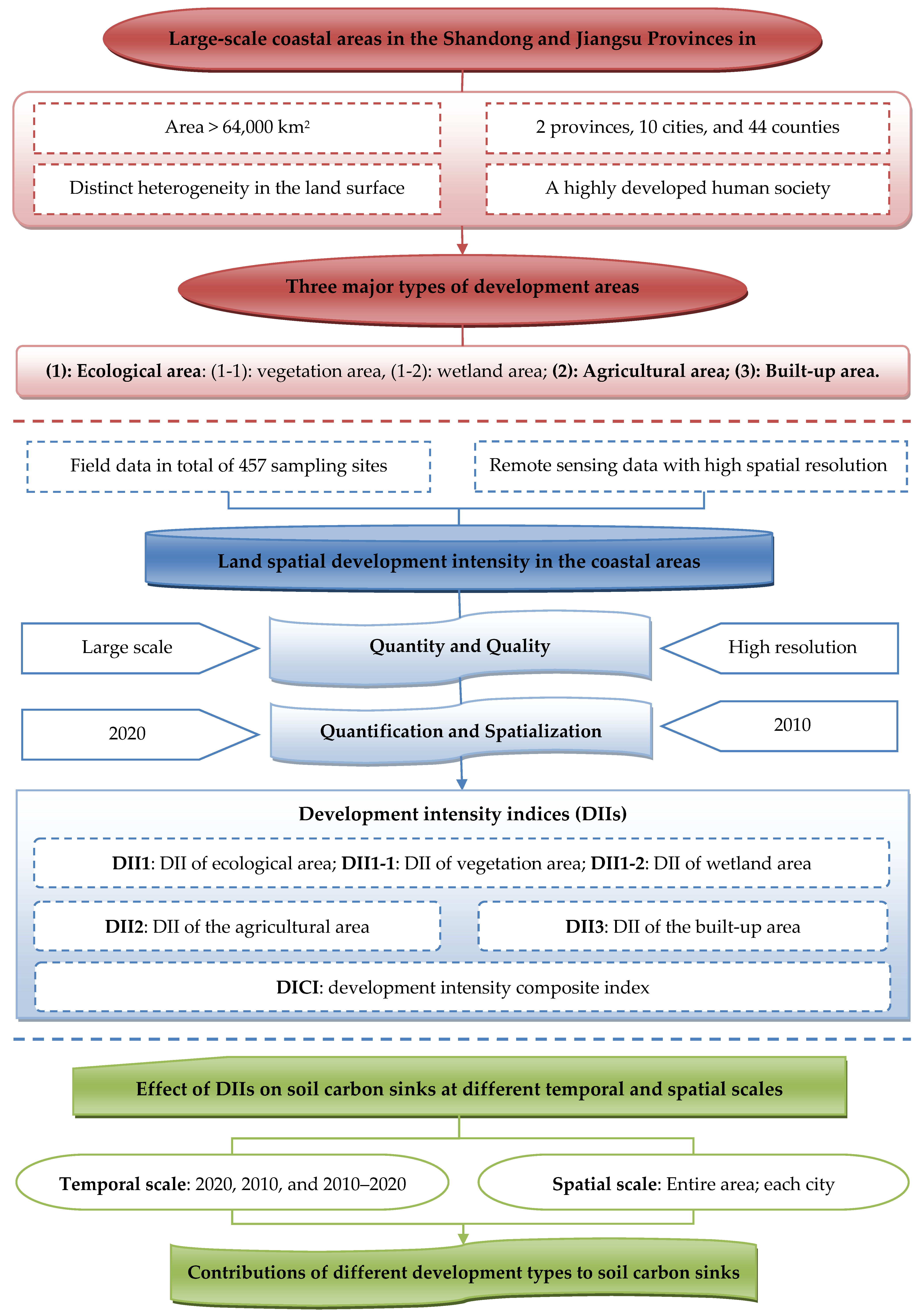
2. Materials and Methods

2.1. Study Area and Data Sources

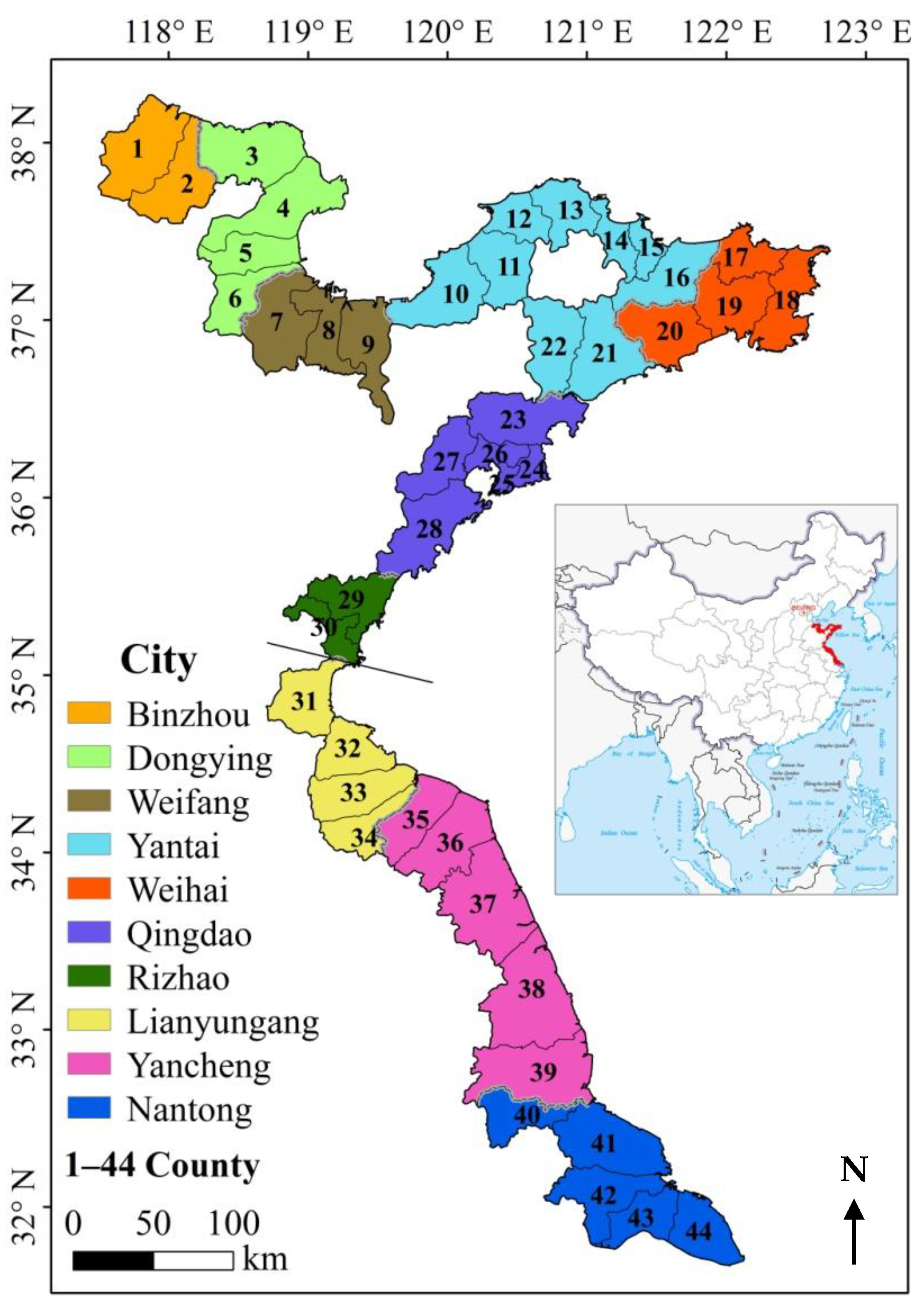
2.1.1. Study Area

The study area encompassed alongshore counties, including counties, county-level cities, and districts, within the Shandong and Jiangsu Provinces in China. The study area ranges from 31°N to 38°N and 117°E to 122°E, and consists of 44 counties in 10 cities in the two provinces (Figure 2). The study area has a warm temperate or subtropical climate that is suitable for crop and natural vegetation growth. The terrain is generally simple and flat in cities 1–3, 9, and 10, owing to the continuous sediment input through China’s two longest rivers, the Yangtze River and the Yellow River, and the coast is mostly muddy in these areas. In contrast, cities 4–7 in Shandong Province and city 8 in Jiangsu Province have undulating terrains and are classified as hilly regions; the coasts in these cities are mostly rocky and sandy.

The study area has a long history of human habitation and exploitation, and urban agglomerations are currently being developed. These 44 counties had more than 37 million permanent residents as of 1 November 2020 [36] (see Figure S1 for a population map of the study area), accounting for 65.15% of the 10 cities, 20.14% of the 2 provinces, and 2.60% of China (1.44 billion). In terms of population density, the 44 counties had a mean population density of 577.35 per km², which is distinctly higher than that of China (150.36 per km²). Moreover, the vast areas in the inner land have long served as an important agricultural hub, producing large amounts of grains, vegetables, and fruits. For instance, County 7 (Shouguang) is a major vegetable-producing area in China, while the Shandong Hilly Region is renowned for its high-quality fruits. Moreover, the study area has abundant ecological resources, with forests and grasslands inland and coastal wetlands in alongshore areas. These ecosystems perform vital ecological functions and serve as key nodes in the regional ecological network, improving ecological connectivity. Within the three major types of development areas, ecological areas are distributed in mountainous areas in the form of forests and grasslands, and along the coastline in the form of wetlands. Forests and grasslands are mainly found in Shandong Hilly Region, while wetlands are generally found on muddy coasts, particularly in the Yellow River Estuary and the Yancheng Coast, which have been designated as National Parks and World Natural Heritage Sites, respectively. Agricultural areas occupied most of the study area. Crops are widely cultivated in the two provinces, particularly in the northwestern part of Shandong Province and almost the entirety of Jiangsu Province. In the Shandong Hilly Region, large-scale fruit trees are planted along with crops. Built-up areas are spread over 44 counties in the form of buildings, roads, ports, and bridges. These areas are continuously distributed in urban areas and scattered in rural areas, exhibiting distinct spatial heterogeneities in terms of area, type, and intensity across different cities and counties within the study area.

2.1.2. Data Sources

Remote sensing: Multiple spectral bands (spatial resolution of 30 m × 30 m) in 2010 and 2020 were collected from the Landsat 5 and 8 satellites, respectively, and employed to generate the spectral reflectance, which was used to calculate the ecological indices. The fused RGB images served as the basis for extracting the coastlines of the study area for the years 2010 and 2020. All remote sensing images were cloud-free and consistent in terms of seasonality. A total of 25 images were selected to cover the entire study area for 2010 and 2020 (see Supplementary Table S1). In addition, GlobeLand30 (https://www.webmap.cn/commres.do?method=globeIndex, accessed on 1 March 2021) provides open-source land cover data, including forests, grasslands, wetlands, croplands, water areas, bare lands, and built-up areas, which were used to identify the three types of development areas. The GlobeLand30 data were derived from a series of remote sensing data obtained from Landsat and the Chinese HJ-1 and GF-1 satellites. The kappa coefficients of 0.78 and 0.82 in 2010 and 2020, respectively, confirm the high accuracy of the data.

Field survey: A total of 457 sampling sites were established and evenly distributed over the study area in September 2020 and May, June, and July 2021 (Supplementary Figures S2 and S3 show a location map and photographs of the sampling sites, respectively). A grid pattern method [37] was employed, and a site was set every 12.5 km to meet the balance of comprehensiveness and cost. In the process of the field survey, the actual positions of the sites were determined by considering the representativeness of the ecological characteristics and field accessibility. Soil samples were collected at the sites, and the soil properties were measured in the laboratory. In the measurement process of soil organic carbon, the measurement conditions were kept consistent across the samples in the 457 sites, ensuring the comparability of the measured results (see Supplementary Table S2 for detailed information on field soil data).

2.2. Quantification of Land Spatial Development Intensity

2.2.1. Scale and Resolution

Spatial scale refers to the scope of the study area, which spanned over 64,000 km² and encompassed a vast and extensive region. Resolution refers to the minimum unit used to quantify the intensity of land spatial development, determining the spatial details, map granularity, and data volume [20,38,39]. The minimum unit should account for the spatial resolution of the data source, such as Landsat and land cover data, which have a spatial resolution of 30 m × 30 m. Therefore, a grid size of 100 m × 100 m was employed as the minimum unit in this study to ensure detailed spatial results while avoiding excessive data volume. The Fishnet tool in ArcGIS 10.6 was used to generate the minimum number of units, resulting in 6,534,950 units in 2020 and 6,441,180 units in 2010.

2.2.2. Quantity and Quality

The land spatial development intensities of the three major types of development areas were quantified based on quantity and quality, following the framework proposed in a previous study on small-scale coastal archipelagic regions in China [6].

(1)

Quantity

Quantity refers to the proportional area of the three major development types in the minimum unit, as derived from the land cover data. The ecological area was divided into two subtypes, namely vegetation and wetland areas, based on differences in their detailed ecological functions and spectral characteristics [24,40]. In the land cover data, the vegetation area consisted of forest and grassland, while the wetland area was limited to wetlands. Additionally, the agricultural area was represented as cropland. Aquaculture ponds were excluded owing to significant differences in their spectral characteristics compared with croplands. The quantity was calculated as follows:

$$\mathrm{Q}\mathrm{T}1=\mathrm{Q}\mathrm{T}1\text{-}1+\mathrm{Q}\mathrm{T}1\text{-}2$$

(1)

$$\mathrm{Q}\mathrm{T}1\text{-}1={\displaystyle \frac{\mathrm{F}\mathrm{A}+\mathrm{G}\mathrm{A}}{\mathrm{T}\mathrm{A}}}$$

(2)

$$\mathrm{Q}\mathrm{T}1\text{-}2={\displaystyle \frac{\mathrm{W}\mathrm{A}}{\mathrm{T}\mathrm{A}}}$$

(3)

$$\mathrm{Q}\mathrm{T}2={\displaystyle \frac{\mathrm{C}\mathrm{A}}{\mathrm{T}\mathrm{A}}}$$

(4)

$$\mathrm{Q}\mathrm{T}2={\displaystyle \frac{\mathrm{C}\mathrm{A}}{\mathrm{T}\mathrm{A}}}$$

(5)

where QT1, QT2, and QT3 are the measured quantities of the ecological, agricultural, and built-up areas, respectively; QT1-1 and QT1-2 are the measured quantities of the vegetation and wetland areas, respectively; FA, GA, WA, CA, and BA are the forest, grassland, wetland, cropland, and built-up areas, respectively; and TA is the total area of the minimum unit.

(2)

Quality

Quality indicates the development level of the three major types per area, and was sourced from multi-spectral remote sensing data obtained from the Landsat 5 and 8 satellites. Three classical ecological indices—the normalized difference vegetation index (NDVI), the soil-adjusted vegetation index (SAVI), and the index-based built-up index (IBI)—were calculated using the methods reported in Huete et al. [41,42,43]. These indices served as the foundation for assessing the quality of the three types of development areas. NDVI directly reflects the vegetation growth and ecological quality [44,45], which makes it suitable for evaluating the quality of ecological areas. SAVI represents both the vegetation conditions and bare soil conditions [46,47], and was employed to assess the quality of agricultural areas, because croplands are seasonally mixed with bare soils. IBI is particularly effective in distinguishing built-up land features [43,48], and was used to assess the quality of built-up areas. The corresponding equations are as follows:

$$\mathrm{Q}\mathrm{L}1=\mathrm{Q}\mathrm{L}1\text{-}1+\mathrm{Q}\mathrm{L}1\text{-}2$$

(6)

$${\displaystyle \mathrm{Q}\mathrm{L}1\text{-}1=\left(\begin{array}{ccc}0& & \mathrm{N}\mathrm{D}\mathrm{V}\mathrm{I}1\text{-}{1}_i\le \mathrm{N}\mathrm{D}\mathrm{V}\mathrm{I}1\text{-}{1}_{1\%}\\ {\displaystyle \frac{\mathrm{N}\mathrm{D}\mathrm{V}\mathrm{I}1\text{-}{1}_i-\mathrm{N}\mathrm{D}\mathrm{V}\mathrm{I}1\text{-}{1}_{1\%}}{\mathrm{N}\mathrm{D}\mathrm{V}\mathrm{I}1\text{-}{1}_{99\%}-\mathrm{N}\mathrm{D}\mathrm{V}\mathrm{I}1\text{-}{1}_{1\%}}}& & \mathrm{N}\mathrm{D}\mathrm{V}\mathrm{I}1\text{-}{1}_{1\%}<\mathrm{N}\mathrm{D}\mathrm{V}\mathrm{I}1\text{-}{1}_i\le \mathrm{N}\mathrm{D}\mathrm{V}\mathrm{I}1\text{-}{1}_{99\%}\\ 1& & \mathrm{N}\mathrm{D}\mathrm{V}\mathrm{I}1\text{-}{1}_i>\mathrm{N}\mathrm{D}\mathrm{V}\mathrm{I}1\text{-}{1}_{99\%}\end{array}\right)}$$

(7)

$$\mathrm{Q}\mathrm{L}1\text{-}2=\left(\begin{array}{ccc}0& & \mathrm{N}\mathrm{D}\mathrm{V}\mathrm{I}1\text{-}{2}_i\le \mathrm{N}\mathrm{D}\mathrm{V}\mathrm{I}1\text{-}{2}_{1\%}\\ {\displaystyle \frac{\mathrm{N}\mathrm{D}\mathrm{V}\mathrm{I}1\text{-}{2}_i-\mathrm{N}\mathrm{D}\mathrm{V}\mathrm{I}1\text{-}{2}_{1\%}}{\mathrm{N}\mathrm{D}\mathrm{V}\mathrm{I}1\text{-}{2}_{60\%}-\mathrm{N}\mathrm{D}\mathrm{V}\mathrm{I}1\text{-}{2}_{1\%}}}& & \mathrm{N}\mathrm{D}\mathrm{V}\mathrm{I}1\text{-}{2}_{1\%}<\mathrm{N}\mathrm{D}\mathrm{V}\mathrm{I}1\text{-}{2}_i\le \mathrm{N}\mathrm{D}\mathrm{V}\mathrm{I}1\text{-}{2}_{60\%}\\ 1& & \mathrm{N}\mathrm{D}\mathrm{V}\mathrm{I}1\text{-}{2}_i>\mathrm{N}\mathrm{D}\mathrm{V}\mathrm{I}1\text{-}{2}_{60\%}\end{array}\right)$$

(8)

$$\mathrm{Q}\mathrm{L}2=\left(\begin{array}{ccc}0& & \mathrm{S}\mathrm{A}\mathrm{V}\mathrm{I}{2}_i\le \mathrm{S}\mathrm{A}\mathrm{V}\mathrm{I}{2}_{1\%}\\ {\displaystyle \frac{\mathrm{S}\mathrm{A}\mathrm{V}\mathrm{I}{2}_i-\mathrm{S}\mathrm{A}\mathrm{V}\mathrm{I}{2}_{1\%}}{\mathrm{S}\mathrm{A}\mathrm{V}\mathrm{I}{2}_{99\%}-\mathrm{S}\mathrm{A}\mathrm{V}\mathrm{I}{2}_{1\%}}}& & \mathrm{S}\mathrm{A}\mathrm{V}\mathrm{I}{2}_{1\%}<\mathrm{S}\mathrm{A}\mathrm{V}\mathrm{I}{2}_i\le \mathrm{S}\mathrm{A}\mathrm{V}\mathrm{I}{2}_{99\%}\\ 1& & \mathrm{S}\mathrm{A}\mathrm{V}\mathrm{I}{2}_i>\mathrm{S}\mathrm{A}\mathrm{V}\mathrm{I}{2}_{99\%}\end{array}\right)$$

(9)

$$\mathrm{QL}3=\left(\begin{array}{ccc}0& & \mathrm{IBI}{3}_i\le \mathrm{IBI}{3}_{1\%}\\ {\displaystyle \frac{\mathrm{IBI}{3}_i-\mathrm{IBI}{3}_{1\%}}{\mathrm{IBI}{3}_{99\%}-\mathrm{IBI}{3}_{1\%}}}& & \mathrm{IBI}{3}_{1\%}<\mathrm{IBI}{3}_i\le \mathrm{IBI}{3}_{99\%}\\ 1& & \mathrm{IBI}{3}_i>\mathrm{IBI}{3}_{99\%}\end{array}\right)$$

(10)

where QL1, QL2, and QL3 are the measured quality values of ecological, agricultural, and built-up areas, respectively; QL1-1 and QL1-2 represent the measured quality values for vegetation and wetland areas, respectively; NDVI1-1_i represents the NDVI value in unit i within the scope of the vegetation area in either 2020 or 2010; NDVI1-1_1% and NDVI1-1_99% are the 1st and 99th percentiles, respectively, of all NDVI values within the vegetation area in 2020 and 2010; NDVI1-2_i is the NDVI value in unit i within the wetland area in 2020 or 2010; NDVI1-2_1% and NDVI1-2_60% are the 1st and 60th percentiles, respectively, of all NDVI values within the wetland area in 2020 and 2010; SAVI2_i is the SAVI value in unit i within the agricultural area in 2020 or 2010; SAVI2_1% and SAVI2_99% are the 1st and 99th percentiles, respectively, of all SAVI values within the agricultural area in 2020 and 2010; IBI3_i is the IBI value in unit i within the scope of the built-up area in either 2020 or 2010; IBI3_1% and IBI3_99% are the 1st and 99th percentiles, respectively, of all IBI values within the built-up area in 2020 and 2010. The selections of upper limits for different ecological indices varied, i.e., the upper limit for NDVI in the QL1-2 calculation was set as the 60th percentile, different from those (the 99th percentile) in the other calculations. The reason underlying the upper limit selection for the QL1-2 calculation is as follows: QL1-2 indicates the quality of wetland areas, which are featured by periodic inundation by seawater and contrasting spectral characteristics across different community types, such as Phragmites australis and Suaeda salsa. These circumstances indicate that wetland areas of high quality do not certainly possess an extremely high NDVI. The spatial distributions of the three types of development areas, in terms of quantity and quality, are shown in Supplementary Figure S4.

2.2.3. Development Intensity Indices

Development intensity indices (DIIs) are proposed to quantify and spatially represent the development intensities of the three major types, in addition to the overall development intensity. The corresponding equations are as follows:

$$\mathrm{D}\mathrm{I}\mathrm{I}1=\mathrm{D}\mathrm{I}\mathrm{I}1\text{-}1+\mathrm{D}\mathrm{I}\mathrm{I}1\text{-}2$$

(11)

$$\mathrm{D}\mathrm{I}\mathrm{I}1\text{-}1=\mathrm{Q}\mathrm{T}1\text{-}1\times \mathrm{Q}\mathrm{L}1\text{-}1$$

(12)

$$\mathrm{D}\mathrm{I}\mathrm{I}1\text{-}2=\mathrm{Q}\mathrm{T}1\text{-}2\times \mathrm{Q}\mathrm{L}1\text{-}2$$

(13)

$$\mathrm{D}\mathrm{I}\mathrm{I}2=\mathrm{Q}\mathrm{T}2\times \mathrm{Q}\mathrm{L}2$$

(14)

$$\mathrm{D}\mathrm{I}\mathrm{I}3=\mathrm{Q}\mathrm{T}3\times \mathrm{Q}\mathrm{L}3$$

(15)

$$\mathrm{D}\mathrm{I}\mathrm{C}\mathrm{I}=\mathrm{D}\mathrm{I}\mathrm{I}1+\mathrm{D}\mathrm{I}\mathrm{I}2+\mathrm{D}\mathrm{I}\mathrm{I}3$$

(16)

where DII1, DII2, and DII3 are the development intensity indices for the ecological, agricultural, and built-up areas, respectively; DII1-1 and DII1-2 are the development intensity indices for the vegetation and wetland areas, respectively; and DICI is the development intensity composite index.

2.3. Effects of Land Spatial Development Intensity on Soil Carbon Sinks

The effects on soil carbon sinks were analyzed from three perspectives: the overall effect, dual-scope gradient analyses, and dual-scope and dual-scheme correlation analyses. The soil organic carbon density (SOCD) in 2020 and 2010 and ΔSOCD across 2010–2020 (SOCD in 2020 minus that in 2010) were used to indicate the soil carbon sink. Spatial data for SOCD covering the entire study area were obtained through digital soil mapping, which integrated point data (field soil data) with area data (remote sensing and land cover data), enabling the conversion from point-based to area-based information. This work was conducted in a previous study, and high accuracy was achieved [20]. Specifically, a predictor system was established for the soil mapping. The system consists of four aspects, namely, ecological indices, landscape composition, landscape configuration, and geographical position, and covers different types of natural and anthropogenic factors influencing the soil carbon; a total of 17 predictors were extracted based on open source remote sensing and land cover data. Then, the 10-fold cross-validation method was employed to conduct the soil mapping and validate the simulation accuracy. The field soil data from the 457 sites were randomly and evenly divided into 10 groups. Each of the 10 groups was considered a validating sample, while the remaining nine groups were considered training samples, with every group serving as the validating sample once. Partial least squares regression was used to implement the simulations through Minitab Statistical Softwarev20 to ensure repeatability. Thus, 10 sets of results were obtained, and the mean value and standard deviation of the 10 sets were used as the final simulation result and uncertainty, respectively. The simulation accuracies were measured using the root mean squared error and Lin’s concordance correlation coefficient, which validated the high accuracy of the soil mapping [20].

The overall effect was determined by analyzing the mean values of SOCD and ΔSOCD across the three major types of development areas. In the dual-scope gradient analyses, DIIs were categorized into different levels, and the variations in SOCD and ΔSOCD across these levels were analyzed within two scopes: the entire study area and each of the 10 cities. Correlation analyses between DIIs and SOCD, and between ΔDIIs and ΔSOCD, were conducted within the two scopes, following two analysis schemes. In Scheme A, correlation analyses were performed using data encompassing the full scope of the analysis. For instance, when the correlation between DII1-1 and SOCD in City 1 was analyzed in Scheme A, DII1-1 and SOCD data for all units in City 1 were employed to conduct the analysis. In Scheme B, the analyses were conducted using data specific to the development areas within the scope of analysis. For example, when analyzing the correlation between DII1-1 and SOCD in city 1 in Scheme B, only data for DII1-1 and SOCD from the vegetation area units in city 1 were used.

3. Results

3.1. Land Spatial Development Intensity in Large-Scale Coastal Areas

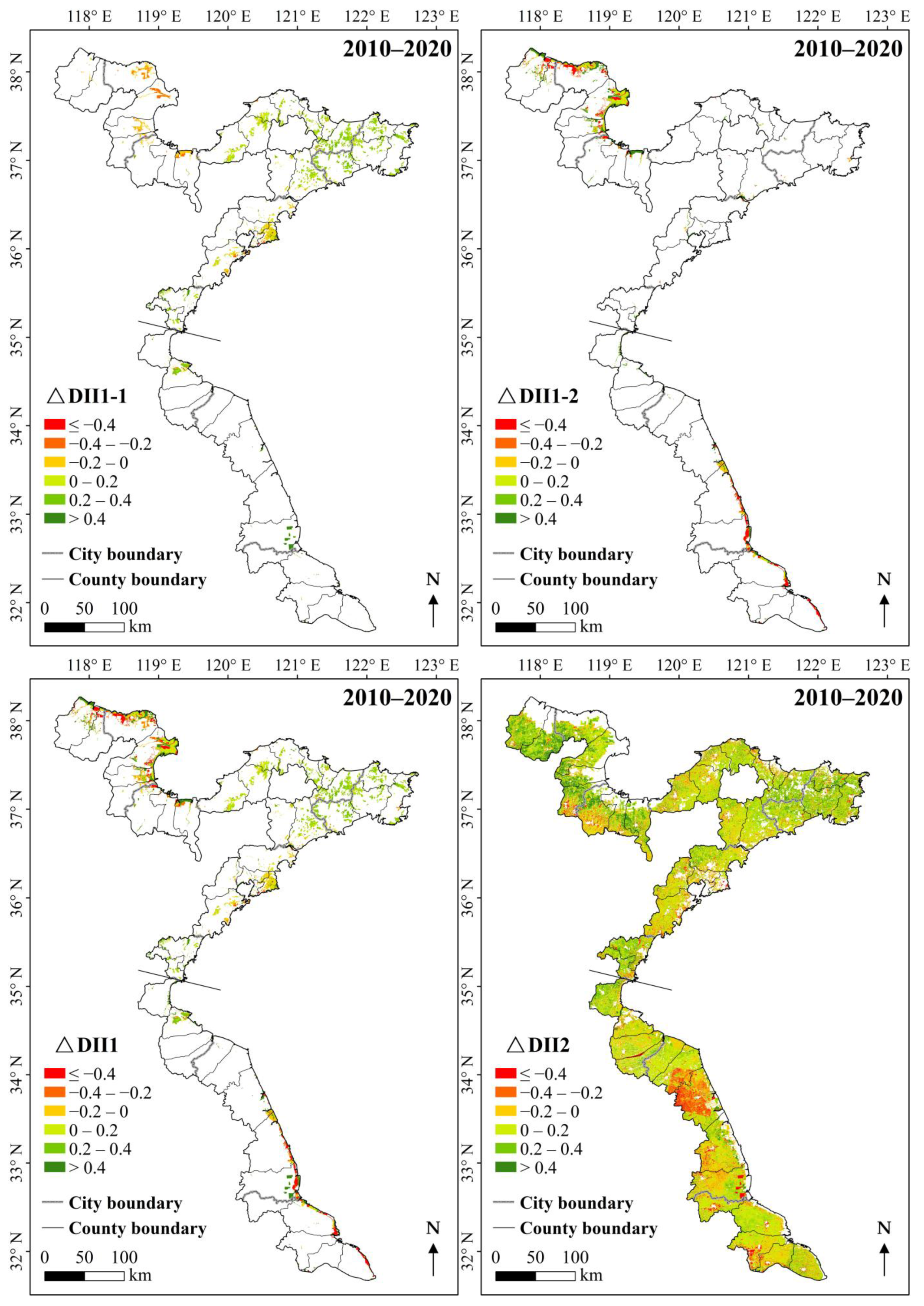
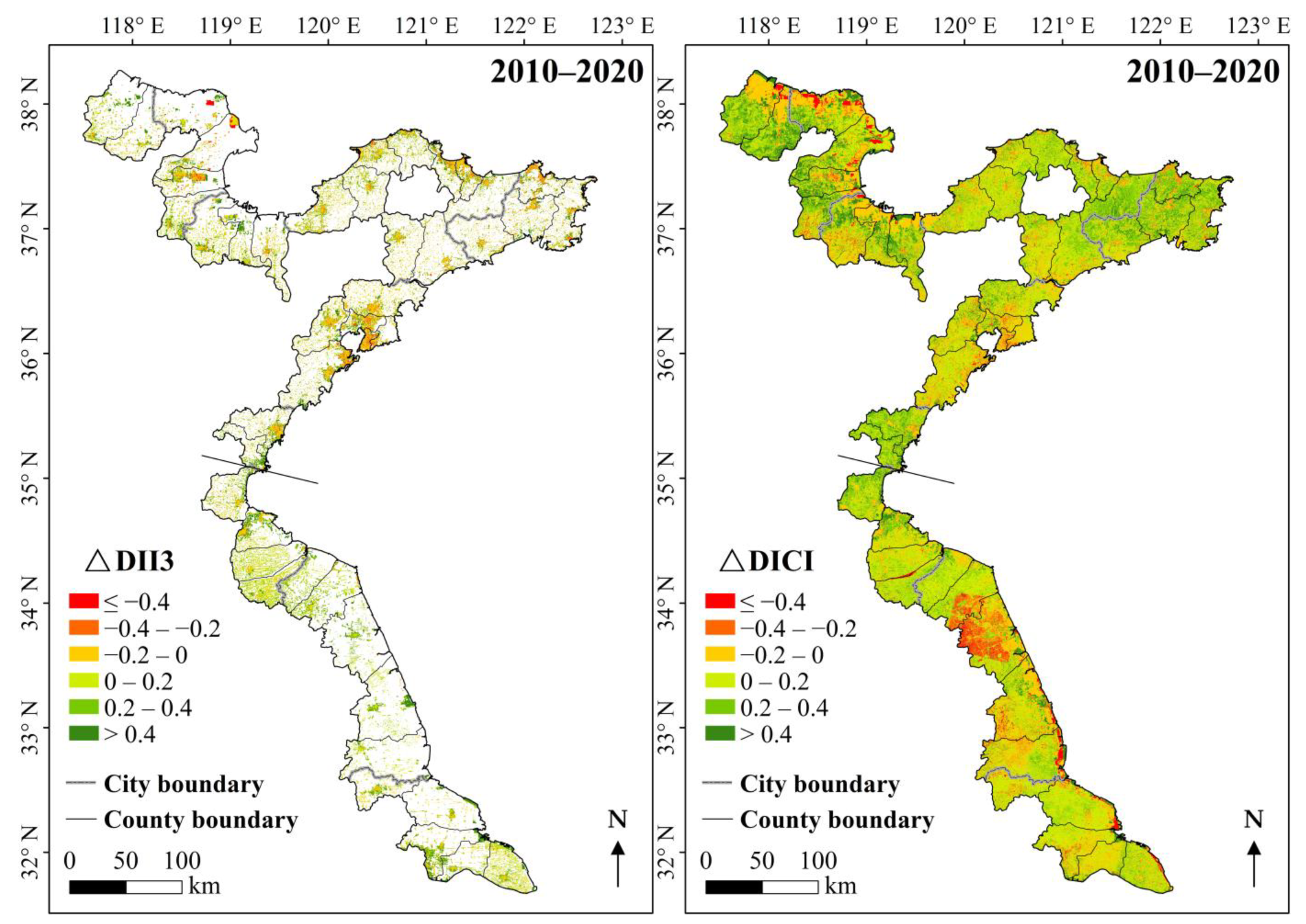
3.1.1. Spatial Distributions of Land Spatial Development Intensity

The spatial distribution of DIIs in 2020 is shown in Supplementary Figure S5. DII1-1 was high in mountainous areas in the eastern part of Shandong Province and the northern corner of Jiangsu Province, while DII1-2 exhibited elevated values in the northwestern part of Shandong Province and the narrow alongshore areas in Jiangsu Province. DII1 combines the spatial characteristics of DII1-1 and DII1-2. DII2 was high in the inner land while low along the coastline. For DII3, high areas were scattered over the study area in patchy formations, with larger patches occurring in urban areas and smaller ones in rural areas. The DICI integrated the above-mentioned indices and exhibited distinct spatial heterogeneity within the study area. The spatial distributions of DIIs in 2010 are shown in Supplementary Figure S6. The indices exhibited spatial patterns similar to those in 2020; however, their overall values were lower than those in 2020. The spatial distributions of ΔDIIs across 2010–2020 are shown in Figure 3. ΔDII1-1 was >0 in most vegetation areas, except the northwestern part of Shandong Province. Areas with ΔDII1-2 > 0 were always near the sea, while those with ΔDII1-2 < 0 were observed on the landward side. ΔDII2 was >0 in most of the study area and <0 in the central part of Jiangsu Province. ΔDII3 was >0 in most built-up areas, with a higher increment observed in rural areas compared with urban areas. ΔDICI combines the spatial characteristics of the above-mentioned indices, and was generally > 0 throughout the study area.

Throughout the study area, all DIIs increased between 2010 and 2020. DII1-1, DII1-2, DII1, DII2, DII3, and DICI increased by 30.34%, 12.18%, 22.29%, 16.33%, 32.55%, and 19.79%, respectively, during 2010–2020.

3.1.2. Land Spatial Development Intensity Along Multiple Gradients and Across Administrative Divisions

Figure 4 shows the changes in DIIs along the gradients of latitude and distance to the coastline (DTC). Along latitudes from 31°N to 38°N, DII1-1 initially increased and then decreased, while DII1-2 followed a pattern of increasing, then decreasing, and finally surging sharply; DII1 generally exhibited an increasing trend, while DII2 exhibited a fluctuating “up-down-up-down” trend; DII3 followed a “down-up-down” trend, and DICI exhibited similar characteristics to DII2. These trends are consistent for both 2020 and 2010. For ΔDIIs, fluctuations were observed from 31°N to 38°N: ΔDII1-1, ΔDII1-2, and ΔDII1 generally followed an “up-down-up” trend and were >0 at intermediate latitudes; ΔDII2 and ΔDICI followed a “down-up-down” trend and were >0, except those at 33°N; ΔDII3 slightly fluctuated and was >0 at all latitudes. Along DTC, DII1-1 initially increased and then decreased with small changes. DII1-2, DII1, and DII3 continuously decreased, whereas DII2 and DICI generally continued to increase in 2020 and 2010. Regarding ΔDIIs, ΔDII1-1 and ΔDII3 exhibited change patterns similar to those of DII1-1 and DII3, respectively, and were constantly >0 at all DTC intervals. ΔDII1-2 and ΔDII1 followed an “up-down-up-down” trend; ΔDII1 was >0 at all intervals, while ΔDII1-2 was >0 except in the 3–10 km intervals. ΔDII2 and ΔDICI first increased and then slightly decreased; ΔDICI was >0 in all intervals, while ΔDII2 was >0 except in the 0–1 km intervals.

The changes in DIIs across administrative divisions are shown in Figure 5. For the 10 cities in 2020 and 2010, DII1-1 was distinctly higher in cities 4–8 compared with the remaining cities, and city 5 achieved the highest DII1-1. DII1-2 exhibits the opposite trends compared with DII1-1, and city 2 has a much higher DII1-2 compared with the nine remaining cities. The differences in DII2 and DII3 across cities are not as large as those in DII1-1 and DII1-2. Cities 9 and 10 exhibited higher DII2 but lower DII3 compared with the remaining cities, while city 6 had the highest DII3. Regarding ΔDIIs, all indices were >0 except ΔDII1-1 in cities 2 and 3, ΔDII1-2 in cities 5, 9, and 10, ΔDII1 in city 10, and ΔDII2 in city 9. Cities 5, 7, and 4 had the highest three ΔDII1-1 and ΔDII1 values; cities 2, 3, and 8 had the highest three ΔDII1-2 values; cities 1, 5, and 7 had the highest three ΔDII2 values; cities 7, 8, and 10 exhibited the highest three ΔDII3 values; and cities 7, 1, and 5 had the highest three ΔDICI values. The changes in DIIs across the 44 counties are shown in Figure 5, where distinct differences can be observed.

3.2. Soil Carbon Sink Effect of Land Spatial Development Intensity

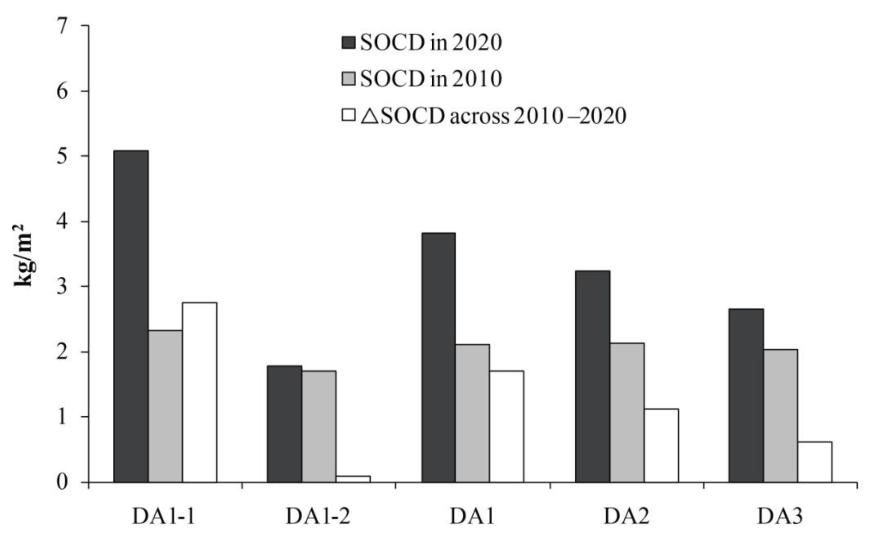
3.2.1. Overall Effect of Different Development Types

Figure 6 shows the SOCDs in the different development areas. The SOCD in 2020 and 2010 exhibited similar change characteristics across different types. Specifically, vegetated areas had the highest SOCD, followed by agricultural and built-up areas, with wetland areas exhibiting the lowest values. However, the differences in SOCD across the different types were much smaller in 2010 than in 2020. Moreover, ΔSOCD was >0 in all development types and exhibited the same change characteristics as those of SOCD in 2020 across different types.

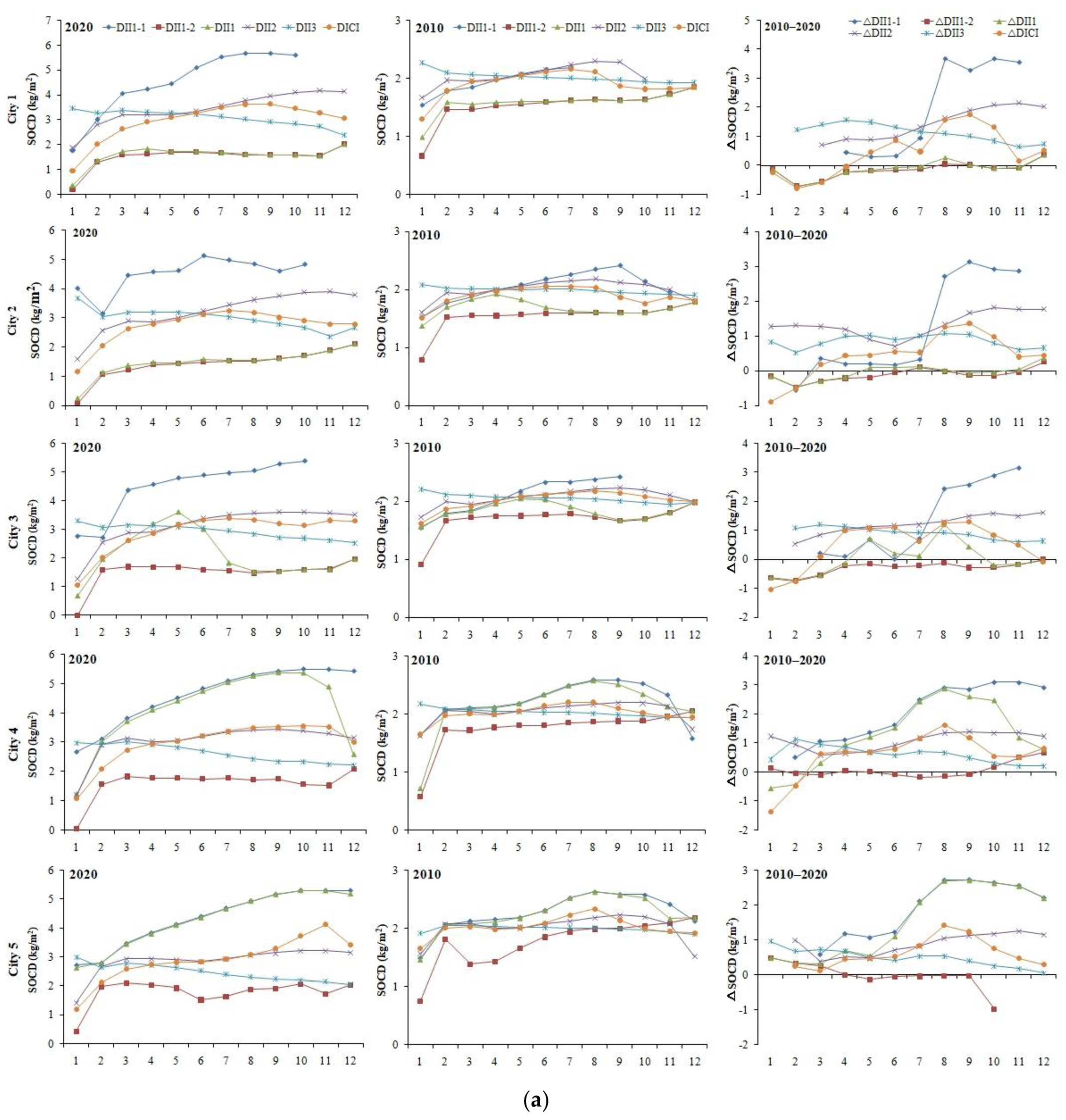
3.2.2. Gradient Analyses Within Two Scopes

Figure 7 shows the changes in SOCD along the different DII levels in the entire study area. In 2020, SOCD continuously increased along the gradients of DII1-1, DII1-2, and DII2, and decreased along the gradient of DII3. SOCD first increased and then decreased along the gradients of DII1 and DICI. The circumstances in 2010 were similar to those in 2020, but two discrepancies were noted: first, the changes in SOCD along the gradients were smaller in 2010 than in 2020; second, SOCD initially increased and then slightly decreased along the gradients of DII1-1 and DII2 in 2010. Regarding ΔSOCD, it continuously increased along the gradient of ΔDII1-1, stayed stable along the gradient of ΔDII1-2, first increased, and then decreased along the gradient of ΔDII1 and ΔDICI, first decreased, then increased, and finally decreased along the gradient of ΔDII2, and continuously decreased with a small change along the gradient of ΔDII3.

Figure 8 shows the changes in SOCD along different DII levels for each of the 10 cities. These characteristics are generally consistent with those in the entire study area. Similar patterns were observed in the 10 cities: ΔSOCD continuously increased and decreased along the gradients of ΔDII1-1 and ΔDII3, respectively; ΔSOCD first increased and then generally decreased along the gradients of ΔDII1 and ΔDICI. The change patterns of ΔSOCD along the gradients of ΔDII1-2 and ΔDII2 varied across different cities. Along the ΔDII1-2 gradient, ΔSOCD generally increased in cities 1–3, fluctuated in cities 4, 6, 7, 9, and 10, and decreased in cities 5 and 8; along the ΔDII2 gradient, ΔSOCD generally increased in cities 1, 3, and 8, initially decreased and then increased in City 7, and initially decreased, then increased, and finally decreased in the remaining cities.

3.2.3. Correlation Analyses Within Two Scopes Using Two Analysis Schemes

The correlation coefficients (CCs) of SOCD with DIIs, along with those of ΔSOCD with ΔDIIs, are presented in Supplementary Table S3. In the entire study area under Scheme A, SOCD exhibited positive CCs with DII1-1, DII1, DII2, and DICI, and negative CCs with DII1-2 and DII3, in 2020 and 2010. The correlation strength, represented by the absolute value of CC (A-CC), was higher for DII1-1, DII2, and DICI than for DII1-2, DII1, and DII3. ΔSOCD had positive CCs with all ΔDIIs except ΔDII3. The A-CCs for ΔDII1-1 were highest among all DIIs; those for ΔDII1, ΔDII2, ΔDII3, and ΔDICI were intermediate, while that for ΔDII1-2 was the lowest. In Scheme B, all CCs were positive except those of SOCD with DII3 in 2020 and 2010, and that of ΔSOCD with ΔDII3 during 2010–2020. The A-CCs were generally higher than those shown in Scheme A. In 2020 and 2010, the incidence of A-CC was high, with the exception of DII1 and DICI. From 2010 to 2020, the A-CC for ΔDII1-1 was distinctly higher than that for the remaining indices.

In each of the 10 cities, the CCs in Scheme A varied in nature and strength for certain DIIs compared with those in the entire study area, whereas the CCs in Scheme B only changed with respect to strength. The changes compared with the circumstances in the entire study area were mainly due to the following points: the CCs for DII1-1 and ΔDII1-1 in cities 1–3, 9, and 10 in Scheme A were distinctly lower than those in the entire study area and the remaining cities; the CCs for ΔDII1-2 in cities 3, 4, and 6–8 in Scheme A, and that in city 5 in Scheme B, became negative; the CCs for DII2 and ΔDII2 in Schemes A and B were generally higher in cities 1–3 than in the entire study area and the remaining cities, while those for ΔDII2 in city 7 in Scheme A and in city 9 in Schemes A and B became negative; the CCs for DII3 were generally consistent with those in the entire study area, except those in cities 1 and 2 in Scheme A.

4. Discussion

4.1. Optimization of Method for Quantifying Land Spatial Development Intensity in Large-Scale Coastal Areas

In this study, the quantity–quality framework was modified based on the factual conditions of the study area to ensure the accuracy and applicability of the framework in large-scale coastal areas. The modifications were based on the following two aspects.

First, the ecological areas were divided into two subtypes: vegetation and wetland areas. In the two coastal archipelagos in the study by Chi et al. [6], wetlands were generally scarce, preventing further subdivision of the ecological area into subtypes. In large coastal areas, forests, grasslands, and wetlands are widespread and distributed across various locations. Forests and grasslands predominantly occur in mountainous areas, where they often intermingle and share similar spectral characteristics as detected by Landsat satellites [11]. Consequently, in this study, they were classified as a single subtype, referred to as the vegetation area. Wetland areas are primarily distributed along the coastline [49]. Because they exhibit differences in terms of location, ecological function, and spectral characteristics compared with the vegetation areas, they were classified as a distinct subtype. The quality values of the two subtypes were calculated separately based on the NDVI to ensure independence, and different percentiles were adopted as the upper limits for the two subtypes in Equations (7) and (8) with consideration to their spectral characteristics.

Second, the methods for measuring the quality values were simplified and optimized. Chi et al. [6] used the Shannon–Wiener index (H’) and NDVI to measure the quality of an ecological area, NDVI to measure that of an agricultural area, and quality coefficients (QCs) to measure that of built-up areas. The H’ value was obtained through field investigation, and the QCs were determined through the detailed functions and floor number of buildings. The difficulty in acquiring accurate H’ and QC values in large-scale coastal areas hinders their application. In this study, plant diversity was recorded in situ, and H’ was calculated for each sampling site. However, the intrinsic correlations between H’ and the predictors sourced by remote sensing were weak, resulting in low accuracy in the spatial simulation of H’. Consequently, it was not possible to generate comprehensive area-wide H’ data for the entire study area. The QCs could not be precisely extracted based on the remote sensing and land-cover data used in this study. Thus, NDVI and IBI, two frequently used ecological indices that are effective in evaluating land features [48,50,51], were employed to measure the quality values of vegetation and built-up areas, respectively. Additionally, because bare land seasonally appears within the agricultural areas in northern China [52], SAVI provides a better indication of the quality of an agricultural area compared with NDVI.

The data required to quantify the large-scale land spatial development intensity were obtained from open-source remote sensing and land cover data, which improved applicability. The 100 m × 100 m resolution maps, with consideration given to both quantity and quality, provided precise spatial details and accurate quantification results, thereby ensuring overall accuracy.

4.2. Spatial Patterns and Influencing Factors of Land Spatial Development Intensity

4.2.1. Spatial Patterns of Land Spatial Development Intensity

The spatial patterns of land spatial development intensity for the three major development types exhibited distinct spatial heterogeneities, which can be summarized as follows:

First, the ecological and built-up areas exhibited “patch” patterns, while the agricultural area exhibited the “area” pattern. These patterns are controlled by long-term common practices, land use policies, and geographic constraints. The patches for ecological areas primarily refer to mountains covered by vegetation in the Shandong Hilly Region and wetlands in certain alongshore areas, such as the Yellow River Delta and Yancheng Wetlands. They perform essential ecological functions in the study area and are fundamental to global bird migration [51,53,54]. The built-up areas consisted of coastal cities with large areas, including the well-known seaside cities of Qingdao, Yantai, and Weihai [55,56], in addition to smaller coastal rural residential areas dispersed throughout the study area. In contrast, agricultural areas dominated the study area, forming the primary landscape matrix in a continuous areal pattern. Agricultural activities have shaped the landscape in the study area for the long term. Under the farmland protection policy, agricultural areas are strictly protected against urbanization, preserving their integrity and spatial pattern.

Second, the coastline serves as a distinctive land feature that shapes the spatial distribution of wetlands and agricultural areas, with their DIIs exhibiting a clear and continuous decrease and increase, respectively, as the DTC increases. Wetland areas developed along the coastline in the form of salt marshes, while agricultural areas in alongshore areas were restrained by soil salinization [57,58,59]. Additionally, built-up areas exhibited a slight decrease as the DTC increased. The locations of coastal cities are affected by the coast type. On rocky and sandy coasts (cities 4–8), cities were consistently established near the sea to exploit marine resources, developing into seaside hubs characterized by tourism and port activities. In contrast, cities on muddy coasts (cities 1–3, 9, and 10) were developed further inland, maintaining some distance from the sea.

Third, the intensity of land spatial development generally increased over the study area in 2010–2020. However, spatial heterogeneity was observed within each development type. The vegetation areas in the Yellow River Delta exhibited a decrease in development intensity, which is attributed to soil salinization stress [52,59]. The wetland areas adjacent to the sea experienced an increase in development intensity, which benefited from the newly formed coastal wetlands resulting from land–sea interactions [60], while those on the landward side exhibited a decrease in development intensity, because natural wetlands were susceptible to occupation and transformed into other development areas [29,61]. Agricultural areas farther from the coastline exhibited a more distinct increase in development intensity compared with those near the coastline. The increase in development intensity for built-up areas was more distinct in rural settlements and coastal engineering regions compared with developed areas.

4.2.2. Factors Influencing Spatial Patterns of Land Spatial Development Intensity

Human activity has been the main factor of change in land surface characteristics, and has driven ecological evolution worldwide in recent decades [62,63,64]. The internal motivations for land utilization are population growth and socioeconomic development. Humans utilize suitable areas for different purposes, including farmlands for food provision, buildings for residence and work, and roads and ports for traffic, all while considering the natural environment in the process. In turn, natural factors constitute the context for exploitation activities and may influence the spatial patterns of different development types [65,66]. The CCs of DIIs with natural factors, that is, the altitude (Al), slope (Sl), and DTC, are presented in Supplementary Table S4. In the entire study area, Al and Sl were positively correlated with DII1-1 and DII1, but negatively correlated with DII1-2, DII2, and DII3, whereas DTC was positively correlated with DII2 and negatively correlated with the remaining indices. However, the correlations were generally weak, except those of Al and Sl with DII1-1, and those of DTC with DII1-2 and DII2. Terrain factors (Al and Sl) influenced only the spatial patterns of the vegetation area, whereas the coastline distinctly influenced the spatial patterns of the wetland and agricultural areas in the entire study area. In each of the 10 cities considered in this study, the effects of terrain factors on DIIs were generally weak in cities with alluvial plains as the main landform type (cities 1–3, 9, and 10), whereas in the remaining cities with eroded hills as the main landform type (cities 4–8), terrain factors had prominent effects on DII1-1, and the effects on DII3 in city 7 were distinct. In contrast, the effects of DTC on DII1-2 and DII2 were particularly distinct in cities 1–3, 9, and 10, which were characterized by muddy coasts, and indistinct in cities 4–8, which typically featured rocky and sandy coasts. Additionally, DTC had a distinct effect on DII3 in city 7. All evidence suggests that natural factors influenced the spatial patterns of land spatial development intensity. However, the degree of influence was limited and varied greatly across different administrative divisions. The effect of terrain factors on vegetation areas was a consequence of differences in the priorities of different development types. Built-up, agricultural, and ecological areas were ranked in descending order of development priority when ecological conservation had not received sufficient attention. As mentioned earlier, humans have utilized land space as extensively as possible for urban construction and agricultural development, and the former has taken priority over the latter in many cases [67,68]. Mountains, where urban construction and agricultural development are challenging, serve as reserved spaces for ecological areas. In recent decades, the prioritization of ecological and agricultural areas has significantly increased within the framework of ecological civilization construction [69] and the requisition–compensation balance of arable land [70]. The coastline has shaped the spatial patterns of wetland and agricultural areas, with wetlands thriving near the coast and agricultural areas developing further inland.

Humans are the fundamental force behind the spatiotemporal variations in land spatial development intensity. The results reveal that DICI increased by 19.79% during 2010–2020 as a result of human effort. The quantity and quality of different development types are controlled by human activities and contribute to changes in DIIs. However, they make contrasting contributions to the increase in DIIs. The quantity values for the ecological, agricultural, and built-up areas decreased by 1.28%, 5.43%, and 36.65%, respectively, whereas the quality values increased by 24.45%, 18.16%, and 28.07%, respectively, from 2010 to 2020. For ecological and agricultural areas, quality rather than quantity was the main driving factor of the DII increase, and quality promotion benefited largely from extensive ecological restoration in China during 2010–2020 [19,20]. Regarding built-up areas, both quantity enlargement and quality enhancement jointly contributed to the DII increase, with the former making a larger contribution. Ongoing urbanization drives an increase in quantity, whereas the development mode of intensive utilization promotes quality [71].

4.3. Contributions of Different Development Types to Spatiotemporal Variations of Soil Carbon Sinks

Different development types with varying DIIs largely determined the spatiotemporal variations in the soil carbon sink, but different development types made different contributions to the spatiotemporal variations. The contributions were measured based on the CCs between the SOCD and DIIs, following the two analysis schemes and accounting for the scale of each development type. These contributions were measured within two scopes, the entire study area and in each of the 10 cities, as follows:

$${\mathrm{I}\mathrm{V}}_i=\left|\mathrm{C}\mathrm{C}1+\mathrm{C}\mathrm{C}2\times \frac{{\mathrm{A}}_i}{\mathrm{T}\mathrm{A}}\right|/2$$

(17)

$${\mathrm{C}\mathrm{t}}_i={\displaystyle \frac{{\mathrm{I}\mathrm{V}}_i}{{\mathrm{I}\mathrm{V}}_s}}\times 100\%$$

(18)

where IV_i is the influencing value of development type i; i = 1, 2, 3, and 4 are the vegetation, wetland, agricultural, and built-up areas, respectively; CC1 and CC2 are the CCs in Schemes A and B, respectively; A_i and TA are the areas of development type i and the total area within the corresponding scope, respectively; Ct_i is the contribution of development type i; and IV_s is the sum of IV within the corresponding scope. The contributions of the different types of development areas to the two scopes are presented in

Table 1. Contributions of different types of development areas to spatiotemporal variations of soil organic carbon density.

Region	2020				2010				2010–2020
	DA1-1	DA1-2	DA2	DA3	DA1-1	DA1-2	DA2	DA3	DA1-1	DA1-2	DA2	DA3
	%	%	%	%	%	%	%	%	%	%	%	%
EA	30.02 +	10.35 −	44.73 +	14.90 −	22.18 +	12.83 −	55.43 +	9.56 −	43.53 +	1.59 +	40.87 +	14.01 −
City 1	2.33 +	11.64 −	84.87 +	1.15 +	1.07 +	5.70 −	89.36 +	3.87 +	5.39 +	7.01 +	80.57 +	7.04 −
City 2	3.22 +	10.01 −	83.90 +	2.86 +	10.65 +	20.82 −	61.32 +	7.20 +	13.70 +	11.65 +	72.89 +	1.76 +
City 3	8.81 +	14.35 −	71.24 +	5.60 −	0.50 −	8.18 −	88.50 +	2.82 −	25.29 +	4.29 −	56.40 +	14.02 −
City 4	47.69 +	6.19 −	19.43 +	26.69 −	48.23 +	3.98 −	31.49 +	16.31 −	49.48 +	1.89 −	33.52 +	15.11 −
City 5	54.82 +	2.14 −	18.71 +	24.33 −	61.97 +	3.06 −	21.03 +	13.94 −	60.26 +	3.13 +	26.30 +	10.30 −
City 6	33.37 +	5.92 −	36.13 +	24.58 −	40.68 +	1.10 −	37.34 +	20.88 −	13.84 +	3.83 −	61.80 +	20.53 −
City 7	48.59 +	5.75 −	20.54 +	25.11 −	38.58 +	1.56 −	46.01 +	13.85 −	66.57 +	7.63 −	0.27 +	25.53 −
City 8	23.19 +	10.32 −	49.15 +	17.34 −	14.21 +	3.35 −	64.89 +	17.55 −	32.97 +	13.54 −	33.67 +	19.81 −
City 9	20.90 +	10.22 −	58.38 +	10.51 −	0.74 −	18.28 −	67.45 +	13.52 −	60.80 +	6.62 +	6.31 −	26.27 −
City 10	7.49 +	14.71 −	55.80 +	22.00 −	0.33 −	23.99 −	57.09 +	18.60 −	17.22 +	7.92 +	49.32 +	25.54 −

ES: Entire area. The numbers for the cities are the same as those in Figure 5. TCC: Total correlation coefficient. DA1-1, vegetation area; DA1-2, wetland area; DA1, ecological area; DA2, agricultural area; DA3, built-up area. Symbols “+” and “−” indicate positive and negative influences, respectively.

. In the entire study area, in 2020 and 2010, the agricultural area made the largest contribution, followed by the vegetation area, while the contributions of the wetland and built-up areas were low. Agricultural and vegetation areas had a positive influence on SOCD, whereas wetland and built-up areas exerted a negative influence. Efforts in management practices, including conservation tillage, straw return, organic fertilizer and green manure application, along with land use and maintenance combinations, and cropland shelterbelt construction, contributed to the increase in SOCD. In terms of variation during 2010–2020, vegetation areas contributed the most, with their contribution being slightly higher than that of agricultural areas. Although the contributions of the wetland and built-up areas remained low, the influence of wetland areas on the SOCD was positive. In each of the 10 cities, the contributions of different development types generally aligned with those observed in the entire study area, though the details varied. Specifically, the contributions of agricultural areas were predominant in cities 1–3, 9, and 10, and relatively low in cities 4–8. The contributions of vegetation areas were higher in cities 4–8 compared with the remaining cities. Generally, wetland areas had low contributions, with positive or negative influences across cities. Built-up areas exerted negative influences in all 10 cities, and the contributions were lower in cities 1 and 2 compared with the remaining cities.

In summary, the increase in the development intensity of ecological and agricultural areas was largely driven by the promotion of ecological quality and improved soil carbon sinks in large-scale coastal areas. The increase in the development intensity of built-up areas led to a reduction in coastal soil carbon. However, this reduction was limited and could be completely bridged and covered by the remarkable increase in soil carbon in other area development types.

5. Conclusions

This study conducted a large-scale quantification of land spatial development intensity in the coastal areas of the Shandong and Jiangsu Provinces in China. The quantity and quality of the three development areas were measured to improve quantification accuracy, using a spatial resolution of 100 m × 100 m. Two time points, 2020 and 2010, were considered as temporal intervals to investigate the spatiotemporal characteristics of land spatial development intensity in the context of extensive ecological restoration. DIIs were introduced to quantify and spatially represent the development intensities of three major area types, namely, ecological, agricultural, and built-up areas, along with the overall development intensity. This approach addressed the first scientific question of this study.

The spatial patterns of the land spatial development intensities for the three major development types exhibited distinct spatial heterogeneity. Coastlines are unique land features that influence the spatial patterns of ecological and agricultural areas. Generally, the land spatial development intensity increased over the study area during 2010–2020, but exhibited distinct spatial variances within each development type. Over the entire study area, the DIIs of the ecological, agricultural, and built-up areas increased by 22.29%, 16.33%, and 32.55%, respectively, and the overall development intensity increased by 19.79%. Quality enhancement was the main driving factor for the increase in DII in ecological and agricultural areas, while both quantity enlargement and quality improvement jointly determined the increase in DII in built-up areas. This answers the second scientific question.

The increase in DIIs contributed to an increase in SOCD between 2010 and 2020. Ecological and agricultural areas had a positive influence on SOCD, while built-up areas exerted a negative influence. The contributions of ecological, agricultural, and built-up areas were 45.12%, 40.87%, and 14.01%, respectively. Furthermore, the contributions of the three major types varied across cities, owing to differences in the natural conditions and socioeconomic environments. This answers the third scientific question.

References

1. Merkens, J.-L.; Reimann, L.; Hinkel, J.; Vafeidis, A.T. Gridded Population Projections for the Coastal Zone under the Shared Socioeconomic Pathways. Glob. Planet. Chang. 2016, 145, 57–66. [Google Scholar] [CrossRef]
2. Lv, Y.; Li, W.; Wen, J.; Xu, H.; Du, S. Population Pattern and Exposure under Sea Level Rise: Low Elevation Coastal Zone in the Yangtze River Delta, 1990–2100. Clim. Risk Manag. 2021, 33, 100348. [Google Scholar] [CrossRef]
3. Pizarro, B.; de Andrés, M.; Barragán, J.M. Coastal Zone in Central Chile, Delimitation Proposal of Valparaiso Region. Ocean Coast. Manag. 2024, 254, 107176. [Google Scholar] [CrossRef]
4. Bazant-Fabre, O.; Bonilla-Moheno, M.; Martínez, M.L.; Lithgow, D.; Muñoz-Piña, C. Land Planning and Protected Areas in the Coastal Zone of Mexico: Do Spatial Policies Promote Fragmented Governance? Land Use Policy 2022, 121, 106325. [Google Scholar] [CrossRef]
5. Yang, D.; Luan, W.; Li, Y.; Zhang, Z.; Tian, C. Multi-Scenario Simulation of Land Use and Land Cover Based on Shared Socioeconomic Pathways: The Case of Coastal Special Economic Zones in China. J. Environ. Manag. 2023, 335, 117536. [Google Scholar] [CrossRef]
6. Chi, Y.; Liu, D.; Wang, C.; Xing, W.; Gao, J. Island development suitability evaluation for supporting the spatial planning in archipelagic areas. Sci. Total Environ. 2022, 829, 154679. [Google Scholar] [CrossRef]
7. Martínez-Megías, C.; Rico, A. Biodiversity Impacts by Multiple Anthropogenic Stressors in Mediterranean Coastal Wetlands. Sci. Total Environ. 2022, 818, 151712. [Google Scholar] [CrossRef]
8. Zhang, Z.; Jiang, W.; Peng, K.; Wu, Z.; Ling, Z.; Li, Z. Assessment of the Impact of Wetland Changes on Carbon Storage in Coastal Urban Agglomerations from 1990 to 2035 in Support of SDG15.1. Sci. Total Environ. 2023, 877, 162824. [Google Scholar] [CrossRef]
9. Zhao, W.; Zhu, K.-H.; Ge, Z.-M.; Lv, Q.; Liu, S.-X.; Zhang, W.; Xin, P. Effects of Plastic Contamination on Carbon Fluxes in a Subtropical Coastal Wetland of East China. J. Environ. Manag. 2023, 345, 118654. [Google Scholar] [CrossRef]
10. Faber-Langendoen, D.; Lemly, J.; Nichols, W.; Rocchio, J.; Walz, K.; Smyth, R. Development and Evaluation of NatureServe’s Multi-Metric Ecological Integrity Assessment Method for Wetland Ecosystems. Ecol. Indic. 2019, 104, 764–775. [Google Scholar] [CrossRef]
11. Zhang, Z.W.; Chi, Y.; Liu, D.H.; Qu, Y.B.; Ma, X.J.; Xing, W.X.; Liu, Z.H. Spatiotemporal Pattern of Landscape Ecological Sensitivity in Coastal Zone in the Last 30 Years: An Empirical Study of Shandong Peninsula, China. J. Coast. Conserv. 2022, 26, 55. [Google Scholar] [CrossRef]
12. Cradock-Henry, N.A.; Flood, S.; Buelow, F.; Blackett, P.; Wreford, A. Adaptation Knowledge for New Zealand’s Primary Industries: Known, Not Known and Needed. Clim. Risk Manag. 2019, 25, 100190. [Google Scholar] [CrossRef]
13. Niu, S.D.; Fang, B. Cultivated Land Protection System in China from 1949 to 2019: Historical Evolution, Realistic Origin Exploration and Path Optimization. China Land Sci. 2019, 33, 1–12. [Google Scholar] [CrossRef]
14. Gao, X.L.; Wu, D.X.; Zhou, K.; Liao, L.W. The Urban Space and Urban Development Boundary under the Framework of Territory Spatial Planning. Geogr. Res. 2019, 38, 2458–2472. [Google Scholar] [CrossRef]
15. Chi, Y.; Zhang, Z.; Xie, Z.; Wang, J. How Human Activities Influence the Island Ecosystem through Damaging the Natural Ecosystem and Supporting the Social Ecosystem? J. Clean. Prod. 2020, 248, 119203. [Google Scholar] [CrossRef]
16. Yue, W.; Hou, B.; Ye, G.; Wang, Z. China’s Land-Sea Coordination Practice in Territorial Spatial Planning. Ocean Coast. Manag. 2023, 237, 106545. [Google Scholar] [CrossRef]
17. Chen, M.X.; Liang, L.W.; Wang, Z.B.; Zhang, W.Z.; Yu, J.H.; Liang, Y. Geographical Thinking on the Relationship between Beautiful China and Land Spatial Planning. Acta Geogr. Sin. 2019, 74, 2467–2481. [Google Scholar] [CrossRef]
18. Crowder, L.B.; Osherenko, G.; Young, O.R.; Airamé, S.; Norse, E.A.; Baron, N.; Day, J.C.; Douvere, F.; Ehler, C.N.; Halpern, B.S.; et al. Resolving Mismatches in U.S. Ocean Governance. Science 2006, 313, 617–618. [Google Scholar] [CrossRef]
19. Chen, X.; Yu, L.; Du, Z.; Xu, Y.; Zhao, J.; Zhao, H.; Zhang, G.; Peng, D.; Gong, P. Distribution of Ecological Restoration Projects Associated with Land Use and Land Cover Change in China and Their Ecological Impacts. Sci. Total Environ. 2022, 825, 153938. [Google Scholar] [CrossRef]
20. Chi, Y.; Liu, D.; Gao, J.; Sun, J.; Zhang, Z.; Xing, W.; Qu, Y.; Ma, X.; Zha, B. Coastal Surface Soil Carbon Stocks Have Distinctly Increased under Extensive Ecological Restoration in Northern China. Commun. Earth Environ. 2023, 4, 373. [Google Scholar] [CrossRef]
21. Brown, M.T.; Vivas, M.B. Landscape Development Intensity Index. Environ. Monit. Assess. 2005, 101, 289–309. [Google Scholar] [CrossRef] [PubMed]
22. Gao, S.; Wang, S. Do Development Zones Increase Urban Land Use Intensity? Empirical Analysis from 235 Cities in China. Appl. Geogr. 2023, 156, 103001. [Google Scholar] [CrossRef]
23. Zheng, H.; Peng, J.; Qiu, S.; Xu, Z.; Zhou, F.; Xia, P.; Adalibieke, W. Distinguishing the Impacts of Land Use Change in Intensity and Type on Ecosystem Services Trade-Offs. J. Environ. Manag. 2022, 316, 115206. [Google Scholar] [CrossRef]
24. Chi, Y.; Zhang, Z.W.; Gao, J.H.; Xie, Z.L.; Zhao, M.W.; Wang, E.K. Evaluating Landscape Ecological Sensitivity of an Estuarine Island Based on Landscape Pattern across Temporal and Spatial Scales. Ecol. Indic. 2019, 101, 221–237. [Google Scholar] [CrossRef]
25. Canelas, J.V.; Pereira, H.M. Impacts of Land-Use Intensity on Ecosystems Stability. Ecol. Model. 2022, 472, 110093. [Google Scholar] [CrossRef]
26. Li, X.; Wu, K.; Yang, Q.; Hao, S.; Feng, Z.; Ma, J. Quantitative Assessment of Cultivated Land Use Intensity in Heilongjiang Province, China, 2001–2015. Land Use Policy 2023, 125, 106505. [Google Scholar] [CrossRef]
27. Xu, Y.; Xu, X.; Tang, Q. Human Activity Intensity of Land Surface: Concept, Methods and Application in China. J. Geogr. Sci. 2016, 26, 1349–1361. [Google Scholar] [CrossRef]
28. Serrano, O.; Lovelock, C.E.; Atwood, T.B.; Macreadie, P.I.; Canto, R.; Phinn, S.; Arias-Ortiz, A.; Bai, L.; Baldock, J.; Bedulli, C.; et al. Australian Vegetated Coastal Ecosystems as Global Hotspots for Climate Change Mitigation. Nat. Commun. 2019, 10, 4313. [Google Scholar] [CrossRef]
29. Li, Y.; Fu, C.C.; Wang, W.Q.; Zeng, L.; Tu, C.; Luo, Y.M. An Overlooked Soil Carbon Pool in Vegetated Coastal Ecosystems: National-Scale Assessment of Soil Organic Carbon Stocks in Coastal Shelter Forests of China. Sci. Total Environ. 2023, 876, 162823. [Google Scholar] [CrossRef]
30. Deb, S.; Mandal, B. Soils and Sediments of Coastal Ecology: A Global Carbon Sink. Ocean Coast. Manag. 2021, 214, 105937. [Google Scholar] [CrossRef]
31. Chi, Y.; Sun, J.K.; Liu, D.H.; Xie, Z.L. Reconstructions of Four-Dimensional Spatiotemporal Characteristics of Soil Organic Carbon Stock in Coastal Wetlands during the Last Decades. Catena 2022, 218, 106553. [Google Scholar] [CrossRef]
32. Owers, C.J.; Rogers, K.; Mazumder, D.; Woodroffe, C.D. Temperate Coastal Wetland Near-Surface Carbon Storage: Spatial Patterns and Variability. Estuar. Coast. Shelf Sci. 2020, 235, 106584. [Google Scholar] [CrossRef]
33. Wang, F.; Wang, T.; Gustave, W.; Wang, J.J.; Zhou, Y.H.; Chen, J.Q. Spatial-Temporal Patterns of Organic Carbon Sequestration Capacity after Long-Term Coastal Wetland Reclamation. Agric. Ecosyst. Environ. 2023, 341, 108209. [Google Scholar] [CrossRef]
34. Hendriks, H.C.M.; van Prooijen, B.C.; Aarninkhof, S.G.J.; Winterwerp, J.C. How Human Activities Affect the Fine Sediment Distribution in the Dutch Coastal Zone Seabed. Geomorphology 2020, 367, 107314. [Google Scholar] [CrossRef]
35. Wang, H.; Zhou, Y.; Wu, J.; Wang, C.; Zhang, R.; Xiong, X.; Xu, C. Human Activities Dominate a Staged Degradation Pattern of Coastal Tidal Wetlands in Jiangsu Province, China. Ecol. Indic. 2023, 154, 110579. [Google Scholar] [CrossRef]
36. National Bureau of Statistics. Bulletin of the Seventh National Population Census in China; National Bureau of Statistics: Beijing, China, 2021.
37. De Gruijter, J.J.; Brus, D.J.; Bierkens, M.F.P.; Knotters, M. Sampling for Natural Resource Monitoring; Springer: Berlin, Germany, 2006. [Google Scholar]
38. Saurette, D.D.; Berg, A.A.; Laamrani, A.; Heck, R.J.; Gillespie, A.W.; Voroney, P.; Biswas, A. Effects of Sample Size and Covariate Resolution on Field-Scale Predictive Digital Mapping of Soil Carbon. Geoderma 2022, 425, 116054. [Google Scholar] [CrossRef]
39. Liang, Z.; Chen, S.; Yang, Y.; Zhao, R.; Shi, Z.; Viscarra Rossel, R.A. National Digital Soil Map of Organic Matter in Topsoil and Its Associated Uncertainty in 1980’s China. Geoderma 2019, 335, 47–56. [Google Scholar] [CrossRef]
40. Fang, Q.; Wang, G.; Liu, T.; Xue, B.-L. Controls of Carbon Flux in a Semi-Arid Grassland Ecosystem Experiencing Wetland Loss: Vegetation Patterns and Environmental Variables. Agric. For. Meteorol. 2018, 259, 196–210. [Google Scholar] [CrossRef]
41. Huete, A.R. A Soil-Adjusted Vegetation Index (SAVI). Remote Sens. Environ. 1988, 25, 295–309. [Google Scholar] [CrossRef]
42. Douaoui, A.E.K.; Nicolas, H.; Walter, C. Detecting Salinity Hazards within a Semiarid Context by Means of Combining Soil and Remote-Sensing Data. Geoderma 2006, 134, 217–230. [Google Scholar] [CrossRef]
43. Xu, H. A New Index for Delineating Built-up Land Features in Satellite Imagery. Int. J. Remote Sens. 2008, 29, 4269–4276. [Google Scholar] [CrossRef]
44. Essaadia, A.; Abdellah, A.; Ahmed, A.; Abdelouahed, F.; Kamal, E. The Normalized Difference Vegetation Index (NDVI) of the Zat Valley, Marrakech: Comparison and Dynamics. Heliyon 2022, 8, e12204. [Google Scholar] [CrossRef]
45. Ruan, L.; Yan, M.; Zhang, L.; Fan, X.; Yang, H. Spatial-Temporal NDVI Pattern of Global Mangroves: A Growing Trend during 2000–2018. Sci. Total Environ. 2022, 844, 157075. [Google Scholar] [CrossRef] [PubMed]
46. Venancio, L.P.; Mantovani, E.C.; do Amaral, C.H.; Usher Neale, C.M.; Gonçalves, I.Z.; Filgueiras, R.; Campos, I. Forecasting Corn Yield at the Farm Level in Brazil Based on the FAO-66 Approach and Soil-Adjusted Vegetation Index (SAVI). Agric. Water Manag. 2019, 225, 105779. [Google Scholar] [CrossRef]
47. Ren, H.; Zhou, G.; Zhang, F. Using Negative Soil Adjustment Factor in Soil-Adjusted Vegetation Index (SAVI) for Aboveground Living Biomass Estimation in Arid Grasslands. Remote Sens. Environ. 2018, 209, 439–445. [Google Scholar] [CrossRef]
48. Hu, X.S.; Xu, H.Q. A New Remote Sensing Index for Assessing the Spatial Heterogeneity in Urban Ecological Quality: A Case from Fuzhou City, China. Ecol. Indic. 2018, 89, 11–21. [Google Scholar] [CrossRef]
49. Zhang, M.; Zhang, H.; Yao, B.; Lin, H.; An, X.; Liu, Y. Spatiotemporal Changes of Wetlands in China during 2000–2015 Using Landsat Imagery. J. Hydrol. 2023, 621, 129590. [Google Scholar] [CrossRef]
50. White, J.G.; Sparrius, J.; Robinson, T.; Hale, S.; Lupone, L.; Healey, T.; Cooke, R.; Rendall, A.R. Can NDVI Identify Drought Refugia for Mammals and Birds in Mesic Landscapes? Sci. Total Environ. 2022, 851, 158318. [Google Scholar] [CrossRef]
51. Yan, J.; Zhu, J.; Zhao, S.; Su, F. Coastal Wetland Degradation and Ecosystem Service Value Change in the Yellow River Delta, China. Glob. Ecol. Conserv. 2023, 44, e02501. [Google Scholar] [CrossRef]
52. Chi, Y.; Sun, J.; Liu, W.; Wang, J.; Zhao, M. Mapping Coastal Wetland Soil Salinity in Different Seasons Using an Improved Comprehensive Land Surface Factor System. Ecol. Indic. 2019, 107, 105517. [Google Scholar] [CrossRef]
53. Wang, C.; Wang, G.; Dai, L.; Liu, H.; Li, Y.; Qiu, C.; Zhou, Y.; Chen, H.; Dong, B.; Zhao, Y.; et al. Study on the Effect of Habitat Function Change on Waterbird Diversity and Guilds in Yancheng Coastal Wetlands Based on Structure–Function Coupling. Ecol. Indic. 2021, 122, 107223. [Google Scholar] [CrossRef]
54. Sun, X.; Shen, J.; Xiao, Y.; Li, S.; Cao, M. Habitat Suitability and Potential Biological Corridors for Waterbirds in Yancheng Coastal Wetland of China. Ecol. Indic. 2023, 148, 110090. [Google Scholar] [CrossRef]
55. Fan, W.; Song, X.; Liu, M.; Shan, B.; Ma, M.; Liu, Y. Spatio-Temporal Evolution of Resources and Environmental Carrying Capacity and Its Influencing Factors: A Case Study of Shandong Peninsula Urban Agglomeration. Environ. Res. 2023, 234, 116469. [Google Scholar] [CrossRef]
56. Huang, L.; Wang, J.; Cheng, H. Spatiotemporal Changes in Ecological Network Resilience in the Shandong Peninsula Urban Agglomeration. J. Clean. Prod. 2022, 339, 130681. [Google Scholar] [CrossRef]
57. Li, H.Y.; Webster, R.; Shi, Z. Mapping Soil Salinity in the Yangtze Delta: REML and Universal Kriging (E-BLUP) Revisited. Geoderma 2015, 237–238, 71–77. [Google Scholar] [CrossRef]
58. Liu, L.P.; Long, X.H.; Shao, H.B.; Liu, Z.P.; Tao, Y.; Zhou, Q.S.; Zong, J.Q. Ameliorants Improve Saline–Alkaline Soils on a Large Scale in Northern Jiangsu Province, China. Ecol. Eng. 2015, 81, 328–334. [Google Scholar] [CrossRef]
59. Guo, B.; Yang, X.; Yang, M.; Sun, D.; Zhu, W.; Zhu, D.; Wang, J. Mapping Soil Salinity Using a Combination of Vegetation Index Time Series and Single-Temporal Remote Sensing Images in the Yellow River Delta, China. Catena 2023, 231, 107313. [Google Scholar] [CrossRef]
60. Fu, Y.; Chen, S.; Ji, H.; Fan, Y.; Li, P. The Modern Yellow River Delta in Transition: Causes and Implications. Mar. Geol. 2021, 436, 106476. [Google Scholar] [CrossRef]
61. Ai, S.; Hu, Y.; Li, J.; Tian, P.; Pu, R.; Liu, Y.; Fan, H. Tracking Economic-Driven Coastal Wetland Change along the East China Sea. Appl. Geogr. 2023, 156, 102995. [Google Scholar] [CrossRef]
62. Halpern, B.S.; Walbridge, S.; Selkoe, K.A.; Kappel, C.V.; Micheli, F.; D’Agrosa, C.; Bruno, J.F.; Casey, K.S.; Ebert, C.; Fox, H.E.; et al. A Global Map of Human Impact on Marine Ecosystems. Science 2008, 319, 948–952. [Google Scholar] [CrossRef]
63. Mahmoud, S.H.; Gan, T.Y. Impact of Anthropogenic Climate Change and Human Activities on Environment and Ecosystem Services in Arid Regions. Sci. Total Environ. 2018, 633, 1329–1344. [Google Scholar] [CrossRef] [PubMed]
64. Xiong, Y.; Mo, S.; Wu, H.; Qu, X.; Liu, Y.; Zhou, L. Influence of Human Activities and Climate Change on Wetland Landscape Pattern—A Review. Sci. Total Environ. 2023, 879, 163112. [Google Scholar] [CrossRef]
65. Sun, Y.; Hou, F.; Angerer, J.P.; Yi, S. Effects of Topography and Land-Use Patterns on the Spatial Heterogeneity of Terracette Landscapes in the Loess Plateau, China. Ecol. Indic. 2020, 109, 105839. [Google Scholar] [CrossRef]
66. Chi, Y.; Sun, J.; Xie, Z.; Wang, J. Soil-Landscape Relationships in a Coastal Archipelagic Ecosystem. Ocean Coast. Manag. 2022, 216, 105996. [Google Scholar] [CrossRef]
67. Bacior, S.; Prus, B. Infrastructure Development and Its Influence on Agricultural Land and Regional Sustainable Development. Ecol. Inform. 2018, 44, 82–93. [Google Scholar] [CrossRef]
68. Lu, L.; Guo, H.; Corbane, C.; Li, Q. Urban Sprawl in Provincial Capital Cities in China: Evidence from Multi-Temporal Urban Land Products Using Landsat Data. Sci. Bull. 2019, 64, 955–957. [Google Scholar] [CrossRef]
69. Xiao, L.; Zhao, R. China’s New Era of Ecological Civilization. Science 2017, 358, 1008–1009. [Google Scholar] [CrossRef] [PubMed]
70. Liu, Y.; Fang, F.; Li, Y. Key Issues of Land Use in China and Implications for Policy Making. Land Use Policy 2014, 40, 6–12. [Google Scholar] [CrossRef]
71. Zhao, J.; Song, Y.; Tang, L.; Shi, L.; Shao, G. China’s Cities Need to Grow in a More Compact Way. Environ. Sci. Technol. 2011, 45, 8607–8608. [Google Scholar] [CrossRef]
Figure 1. Framework for quantifying land spatial development intensity and its effect on soil carbon sinks in coastal areas.
Remotesensing 17 01197 g001
Figure 2. Administrative divisions of study area: Shandong Province and Jiangsu Province are above and below the oblique line, respectively. The names of 44 counties (including county, county-level city, and district) are as follows: 1. Wudi County; 2. Zhanhua District; 3. Hekou District; 4. Kenli District; 5. Dongying District; 6. Guangrao County; 7. Shouguang City; 8. Hanting District; 9. Changyi City; 10. Laizhou City; 11. Zhaoyuan City; 12. Longkou City; 13. Penglai District; 14. Fushan District; 15. Municipal District; 16. Muping District; 17. Huancui District; 18. Rongcheng City; 19. Wendeng City; 20. Rushan City; 21. Haiyang City; 22. Laiyang City; 23. Jimo District; 24. Laoshan District; 25. Municipal District; 26. Chengyang District; 27. Jiaozhou City; 28. Huangdao District; 29. Donggang District; 30. Lanshan District; 31. Ganyu District; 32. Municipal District; 33. Guanyun County; 34. Guannan County; 35. Xiangshui County; 36. Binhai County; 37. Sheyang County; 38. Dafeng District; 39. Dongtai City; 40. Hai’an City; 41. Rudong County; 42. Municipal District; 43. Haimen District; and 44. Qidong City.
Remotesensing 17 01197 g002
Figure 3. Spatiotemporal variations of land spatial development intensity from 2010 to 2020: ΔDII1-1 indicates the variation of DII1-1 between 2020 and 2010, calculated as DII1-1 in 2020 minus that in 2010. The same situations apply to the other indices. DII1-1: development intensity index of vegetation area; DII1-2: development intensity index of wetland area; DII1: development intensity index of ecological area; DII2: development intensity index of agricultural area; DII3: development intensity index of built-up area; DICI: development intensity composite index.
Remotesensing 17 01197 g003aRemotesensing 17 01197 g003b
Figure 4. Intensity of land spatial development along gradients of latitude and distance to coastline. DTC: distance to coastline. DII1-1: development intensity index of vegetation area; DII1-2: development intensity index of wetland area; DII1: development intensity index of ecological area; DII2: development intensity index of agricultural area; DII3: development intensity index of built-up area. DICI: development intensity composite index.
Remotesensing 17 01197 g004
Figure 5. Land spatial development intensity in different cities and counties: DII1-1: development intensity index of vegetation area; DII1-2: development intensity index of wetland area; DII1: development intensity index of ecological area; DII2: development intensity index of agricultural area; DII3: development intensity index of built-up area. DICI: development intensity composite index. City 1: Binzhou; city 2: Dongying; city 3: Weifang; city 4: Yantai; city 5: Weihai; city 6: Qingdao; city 7: Rizhao; city 8: Lianyungang; city 9: Yancheng; city 10: Nantong. The numbers of counties are the same as those in Figure 2.
Remotesensing 17 01197 g005
Figure 6. Soil organic carbon density in different types of development areas: SOCD: soil organic carbon density. DA1-1: vegetation area; DA1-2: wetland area; DA1: ecological area; DA2: agricultural area; DA3: built-up area.
Remotesensing 17 01197 g006
Figure 7. Changes in soil organic carbon density across different levels of development intensity indices in entire study area: DII1-1: development intensity index of vegetation area; DII1-2: development intensity index of wetland area; DII1: development intensity index of ecological area; DII2: development intensity index of agricultural area; DII3: development intensity index of built-up area. DICI: development intensity composite index. The numbers under the lateral axis indicate the different levels of the indices. For 2020 and 2010: 1: DII = 0; 2: DII ∈ (0, 0.1); 3: DII ∈ [0.1, 0.2); 4: DII ∈ [0.2, 0.3); 5: DII ∈ [0.3, 0.4); 6: DII ∈ [0.4, 0.5); 7: DII ∈ [0.5, 0.6); 8: DII ∈ [0.6, 0.7); 9: DII ∈ [0.7, 0.8); 10: DII ∈ [0.8, 0.9); 11: DII ∈ [0.9, 1); 12: DII = 1. For 2010–2020: 1: ΔDII = −1; 2: ΔDII ∈ (−1, −0.8); 3: ΔDII ∈ [−0.8, −0.6); 4: ΔDII ∈ [−0.6, −0.4); 5: ΔDII ∈ [−0.4, −0.2); 6: ΔDII ∈ [−0.2, 0); 7: ΔDII ∈ [0, 0.2); 8: ΔDII ∈ [0.2, 0.4); 9: ΔDII ∈ [0.4, 0.6); 10: ΔDII ∈ [0.6, 0.8); 11: ΔDII ∈ [0.8, 1); 12: ΔDII = 1.
Remotesensing 17 01197 g007
Figure 8. (a). Changes in soil organic carbon density along different levels of development intensity indices in cities 1–5. DII1-1: development intensity index of vegetation area. DII1-2: development intensity index of wetland area. DII1: development intensity index of ecological area. DII2: development intensity index of agricultural area. DII3: development intensity index of built-up area. DICI: development intensity composite index. The numbers under the lateral axis indicate the different levels of indices, as in Figure 7. (b) Changes in soil organic carbon density along different levels of development intensity indices in cities 6–10: DII1-1: development intensity index of vegetation area. DII1-2: development intensity index of wetland area. DII1: development intensity index of ecological area. DII2: development intensity index of agricultural area. DII3: development intensity index of built-up area. DICI: development intensity composite index. The numbers under the lateral axis indicate the different levels of indices, as shown in Figure 7.
Remotesensing 17 01197 g008aRemotesensing 17 01197 g008b