Abstract
Compared to traditional remote sensing technology, video satellites have unique advantages such as real-time continuous imaging and the ability to independently complete staring observation. To achieve effective staring control, the satellite needs to perform attitude maneuvers to ensure that the target’s projection stays within the camera’s visual field and gradually reaches the desired position. The generation of image-based control instructions relies on the calculation of projection coordinates and their rate of change (i.e., visual velocity) of the projection point on the camera’s image plane. However, the visual velocity is usually difficult to obtain directly. Traditional calculation methods of visual velocity using time differentials are limited by video frame rates and the computing power of onboard processors, and is greatly affected by measurement noise, resulting in decreased control accuracy and a higher consumption of maneuvering energy. In order to address the shortcomings of traditional calculations of visual speed by time difference methods, this paper proposes a control method based on the estimation of visual velocity, which achieves real-time calculation of the target’s visual speed through adaptive estimation; then, the stability of the closed-loop system is rigorously demonstrated. Finally, through simulation comparison with the traditional differential method, the results show that the proposed method has an improvement in attitude accuracy for about 74% and a reduction in energy consumption by about 77%.
1. Introduction
Video satellites have the characteristics of agile attitude maneuvering, real-time continuous video imaging, and the ability to independently complete tracking and observation [1,2,3]. They have unique advantages compared with traditional remote sensing satellites [4]. They can achieve continuous staring observation of ground or space targets, and have broad application prospects in resource exploration, Earth observation, and other fields. Due to the above features, many countries and agencies have attached a greater importance to the research of video satellites, and have successively launched a batch of them in recent years, such as the Skybox [5], LAPAN-TUBSA [6], SkySat [7], Tiantuo-2 [8], and Jilin-1 [9,10] satellites, etc., as a supplement to traditional remote sensing observation methods or ground-based observation methods.
The staring control of video satellites usually requires the camera’s optical axis to point towards the direction of the target, which can make the target projection stay at the center position of the camera’s imaging plane and achieve ideal observation results. It can also avoid the target from leaving the camera’s field of view by leaving a certain distance to the edge of the image plane, ensuring the continuity of the tracking observation. Due to the orbital motion of the video satellite, displacement between the target and the satellite exists. In order to achieve tracking and observation, it is necessary to design attitude controllers for the video satellite.
Early research on video satellite tracking and control required the prior geographic position information of ground targets as the input of the attitude controller in order to calculate attitude errors and then implement staring control [1,11,12,13,14]. This type of method is a location-based tracking control that does not involve the image information obtained by the camera, so the prior position information of the target is required. This means that it cannot be applied to the observation of non-cooperative targets, due to the lack of prior information. Therefore, some scholars have started to conduct research on the staring control of video satellites based on visual image feedback [11,15,16,17,18,19,20,21], which can be applied to the observation of both cooperative and non-cooperative targets.
The methods used in the above studies all assume that the parameters of the onboard camera system are precisely calibrated. However, the calibration of cameras in orbit is difficult and time-consuming, making it difficult to meet the rapid response requirements of increasingly complex space-based observation tasks. At the same time, during the long duration of orbit motion, the camera is affected by factors such as heat and vibration, and its optical properties may also deviate to the nominal value. Adopting a method under the assumption of precise camera calibrations will affect the tracking and control accuracy. Currently, two main methodologies are being utilized to resolve the issue. One is the model revision method, which compensates for the parameter deviation caused by some specific factors (thermal deformation [22], geometric deformation of photosensitive elements [23], etc.) to a certain extent, but is difficult to meet the demand for fast response. The other method compensates for the impact of parameter deviations using control algorithms. At present, this method has been studied (to some extent) in the fields of ground robots [24,25,26,27,28,29,30,31,32] and drones [33,34,35,36,37,38]. However, research on the tracking and control of targets by video satellites with uncalibrated in-orbit cameras is still relatively scarce.
The image-based control method requires establishing the relationship between the relative position of the target with the video satellite and its projection point coordinates on the camera’s imaging plane. The control law is calculated using the deviation between the present projection point and the expected point. Then, under the control maneuver, the attitude of the video satellite is changed, gradually moving the target projection point to the expected position. Therefore, the generation of control instructions depends on the calculation of the change rate of projection point coordinates; that is, the visual speed information. However, in reality, visual speed is difficult to measure directly. In order to calculate the visual speed and use it as an input for the controller, it can be indirectly obtained using traditional methods, by calculating the time differential of the pixel coordinates; that is, the differential calculated value of the visual velocity is obtained by dividing the variation in the target’s projected coordinates at adjacent moments by the time interval. The differential operation accuracy is directly affected by the differences in the time intervals. The smaller the time interval, the higher the visual velocity accuracy obtained. However, the time interval is first limited by the video frame rate of the onboard cameras; for example, the video frame rate of Tiantuo-2 and Jilin-1 is 25 frames per second, while the frame rate of the Surrey V-1C video satellite can reach 100 frames per second. Therefore, even with the same control law, different control effects could occur on video satellites with different frame rate shooting capabilities. Moreover, differential operation is also influenced by algorithms and hardware, with significant differences in image processing speeds between different algorithms and hardware which limit the rapid response capability of video satellites. In addition, the measured pixel coordinates inevitably contain noise effects, and the time difference operation will amplify the impact of noise, which can further affect the control accuracy. Therefore, the visual speed obtained with these differences is not only affected by a lack of smoothness, but is also susceptible to noise, which can reduce control accuracy and stability. Thus, it is necessary to design corresponding adaptive visual tracking control methods for situations where visual velocity is treated as an unknown variable without using differential methods. However, there is still relatively little research on how to obtain the visual velocity when it is difficult to acquire.
This manuscript comprehensively considers the tracking control of video satellites under the conditions of uncalibrated cameras and unknown visual velocity. First, we redesign the control law proposed in Ref. [39] by constructing an adaptive law to estimate the visual speed of the target which does not rely on differential calculations as in the reference. Using real-time camera parameter estimation, the reference attitude trajectory, parameter update law, and tracking controller are all calculated using visual speed estimation values. Simulations demonstrate improved noise robustness and smoother tracking compared to the results in the original reference.
The remaining part of the paper proceeds as follows. In Section 2, the physical models of this article, including the video satellite motion model and camera projection model, are established. In Section 3, we describe the model for estimating visual velocity, redesign the control law, and rigorously prove the stability of the closed-loop system. In Section 4, we conduct comparisons and analyses with the differential calculation of visual velocity through simulation, and we end with some conclusions and open problems in Section 5.
2. Problem Formulation
This section establishes the mathematical models that were used. In order to simplify the article, some formulas have been derived from existing models in Ref. [39], and some of the detailed derivation processes can be found in the original literature. To improve readability, some key variables used in this section are summarized in Table 1.

Table 1.
Variables and their definitions.
2.1. Kinematics and Dynamics of Video Satellite
The kinematic and dynamic equations describe the motion characteristics of the video satellite. Under the assumption of a rigid body, the kinematic and dynamic equations of the video satellite are given by
where J is the moment of inertia of the video satellite, is a 3-order unit matrix, and are the angular velocity and attitude quaternion of the video satellite, and is the attitude control torque. The operator is a 3 × 3 skew-symmetric matrix with diagonal elements of 0, with the form of
2.2. Staring Observation Model
When a video satellite performs earth-staring observation tasks, it requires the camera’s optical axis to point towards the ground target, as shown in Figure 1. denotes the satellite’s Earth-centered inertial (ECI, ) position and denotes the transfer matrix from ECI to the satellite’s body frame . Then, the observation model is
where is the extended Euler transform matrix from the inertial frame to the satellite’s body frame.
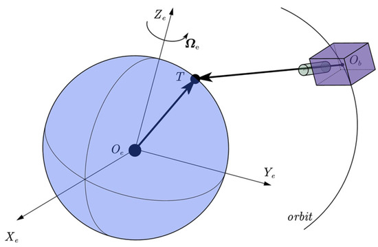
Figure 1.
The diagram of satellite staring observation of ground target T.
After establishing the staring observation model, it is necessary to convert the position relationship of the target relative to the satellite into a projection relationship. In the following text, the intrinsic and extrinsic projection models of the camera are established separately, and then the projection kinematics model is ultimately derived.
2.3. Camera Intrinsic Model
As shown in Figure 2, the observation target T in the camera frame is denoted by and its projection coordinate in the image plane is . Then, the projection model of the target is
where , is the angle between the two axes of the image plane and is the intersection point of the optical axis and the image plane.
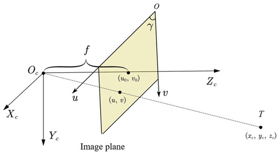
Figure 2.
Camera intrinsic model.
2.4. Camera Extrinsic Model
As shown in Figure 3, the transformation between and can be described by
where is the extended Euler transform matrix between the satellite’s body frame to the onboard camera frame.
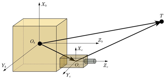
Figure 3.
Camera extrinsic model.
2.5. The Projection Kinematics of Staring Imaging
After obtaining the two projection models, the position of the target observed by the camera at the projection point on the imaging plane can be determined. Next, we will separate the projection point’s coordinates to obtain the kinematics of staring imaging.
Combining Equations (5) and (6), we can obtain the relation between the position of the observation target in ECI and its projection coordinates on the image plane; this is
where is called the projection matrix, which establishes the relationship between the position of the target in ECI and the coordinates of the camera projection point. Its elements are denoted as .
Expand the matrix by rows and define it as
where denotes the first two rows of projection matrix , and is the third row. Then, Equation (7) can be rewritten as
Denote the first three elements of and first three columns of as and , respectively. The differentiative of and can be expressed and simplified as [39]
Equations (10) and (11) are called the staring imaging kinematics. is the rate of change in the coordinates of the target on the imaging plane of the onboard camera over time, i.e., the visual velocity.
3. Design of Adaptive Control Law
3.1. Estimation of Visual Velocity
Visual velocity is a crucial input for the controller. When it is unknown, real-time estimation is required. In the manuscript, we define as the estimated value of a. Then, according to Equation (10), the current estimated value of the real-time visual velocity can be expressed as
Combining Equations (10) and (12), the estimation error of visual velocity is defined as
where is the estimation of the elements in matrix N and is the estimation error, which is the same as the definition in Ref. [39].
Through the intermediate step of the above equation, it can be seen that the estimation error expression of visual velocity contains the parameter “estimation error” (), so it can be represented by linearization. It should be noted that after extracting , the remaining expressions still contain parameter estimation values, so is related to the parameter estimation results .
3.2. Reference Attitude Trajectory
When designing the controller, the deviation between the current state and the expected state is usually used as its input. Due to the difficulty in directly calculating the expected angular velocity , we indirectly calculated the attitude error by defining a reference attitude trajectory. In Ref. [39], the reference attitude trajectory , reference image tracking error , and reference angular velocity tracking error are defined as
where is the image error between the current projected position and the expected position. is defined as
It can be seen that is determined solely by and is unrelated to the unknown visual velocity . Therefore, there is no need to re estimate . However, is related to , so it is necessary to use the estimated values of visual velocity instead, which leads to
By combining Equations (12) and (17), the estimated image tracking error satisfies
By taking the derivative of Equation (17), we can obtain the rate of change of the reference angular velocity
It can be seen that some terms in (20) do not include visual velocity, while the third term that includes visual velocity can be expressed in a linear form (since ). Therefore, the reference angular acceleration can be expressed in a simplified way:
where is part of the expression of , which is independent of visual velocity. The matrix is defined by linearizing the visual velocity and removing the estimated depth. Due to the unknown , the estimated value is substituted into (21) to get
Subtracting Equation (21) from Equation (22), the difference between the reference angular acceleration and its estimated value can be obtained by combining them with Equation (13), resulting in
3.3. Design of Control Law
3.3.1. Parameter Definition and Estimation Law
Firstly, we need to calculate the estimation error, including the projection coordinate estimation error and camera parameter estimation error. The estimated projection error is defined in the same way as Ref. [39] with the expression of
The parameter update law is designed as
where , , and are all positive definite matrix.
The key difference from the parameter update law in Ref. [39] is the first term, which is used to simplify the process of closed-loop stability proof. and are selected to make the system stable. The stability proof will be conducted in the following text.
3.3.2. Staring Controller Design
By redesigning the controller in Ref. [39] and using the estimated parameters as input, the designed control law can be obtained as
where , , , and are positive definite matrix. Substituting the control law expression into (2), we can obtain
Combining Equation (23), the following expression yields
3.3.3. Stability Analysis
Choosing an appropriate positive-definite Lyapunov function and analyzing its time derivative is a common method for analyzing the stability of the system. Here we construct the following two non-negative functions to conduct stability analysis:
Taking the derivative of , we can obtain
Substituting Equation (19) into the above equation, we can obtain
Taking the derivative of and combining it with Equation (25), we can obtain
The Lyapunov function is taken as ; then, we can obtain
Next, we will analyze the derivative of the Lyapunov function to determine the stability of the closed-loop system. According to Equation (11), and are both bounded functions; therefore, it is assumed that
According to the property that the dot product of vectors is less than or equal to the product of the vector module length, by scaling Equation (34), we can obtain
represents the minimum value of , when the following inequality holds
We have
where , , , and are the minimum eigenvalues of , , , and , is the maximum eigenvalue of . Thus, is bounded, and so are , , , and . According to Equation (25), the derivative of the estimated parameter values is also bounded. Furthermore, it can be inferred that the derivative of the estimated projection error is also bounded.
According to Equation (22), it can be inferred that is also a bounded function, and so is . Therefore, combining the attitude dynamics of the video satellite, the boundedness of the angular acceleration can be obtained. Based on the above analysis, it can be concluded based on Barbalat’s lemma that
that is
According to Equation (24), since the parameter estimation values will not all be zero, when is approaching 0, the depth estimation value cannot be zero, resulting in
Due to the inclusion of and in , it is not yet possible to determine the convergence of the pixel error. Next, we will further prove that the projection point will converge to the expected position in the image plane. By estimating the pixel coordinates through parameter estimation values, the estimated pixel coordinates can be defined as
When is approaching 0, we have
Therefore, according to Equations (42) and (43), it can be concluded that
According to the differentiation rule
By substituting Equation (40) obtained from Barbalat’s lemma into the expression of the parameter update law (25), it can be seen that the derivative of the estimated parameter value also tends to zero. Therefore, by substituting it into the above equation, we obtain
According to Equations (45) and (47), we get
The above equation indicates that the estimated visual velocity will eventually approach the actual visual velocity. Therefore, it can be inferred that
This means that the visual tracking error will eventually converge. Therefore, under the designed adaptive visual tracking controller, the estimated visual velocity gradually approaches the actual value, the projection of the ground target gradually approaches the expected coordinates, and then finally stabilizes at the center of the image.
Based on the above derivation process, it can be seen that the process of proving the convergence of visual velocity estimation values does not rely on the sampling time step. Therefore, this method can effectively estimate the visual velocity under different video frame rates, thereby achieving effective tracking of the target. However, for the differential time calculation method, its calculation accuracy of visual velocity will be directly related to the video frame rate. Therefore, this method has stronger universality and can achieve more accurate visual velocity estimation for satellites with different video sampling capabilities. Next, we will validate this method through simulation comparison.
4. Simulation
4.1. Parameter Setting
In this section, we compare the proposed controller based on visual velocity estimation with the differential method in Ref. [39] for ground target observation.
The initial (12 January 2025 12:30:00 UTC) location of the ground target is shown in Table 2. The orbit elements of the video satellite are shown in Table 3. The parameters of the onboard camera are given in Table 4, in which represents the Euler transformation matrix in the order of 3-2-1. The parameters of the controller designed in this paper are shown in Table 5. The compared controller parameters are consistent with Ref. [39]. The nominal parameters are initially real states of the camera and are used as the initial estimated values. In long term obit motion, the actual parameters deviate from the nominal values. is the desired projection position of the observed target. The initial attitude motion states of the satellite are shown in Table 6. It is assumed that the maximum control torque of the actuator is 0.1 N·m; that is, holds for .
Table 2.
Location of the observed ground target.
Table 3.
Orbit elements of the video satellite.
Table 4.
Camera parameters.
Table 5.
Controller parameters.
Table 6.
Initial attitude motion states of the satellite.
The simulation comparative analysis includes two parts. First, the results of the traditional time difference method under different time steps are analyzed with the visual velocity estimation method. Then, we add noise in the pixel coordinates to simulate measurement errors in the image processing process to comparatively analyze the effects of the two methods.
In order to quantitatively analyze the performance of the two methods, we define two indicators that characterize the energy consumption during the control process and the terminal stability, with the expressions of
where and are the duration of the simulation and stable stage, respectively. It can be seen that can characterize the energy consumption during the control process and can indicate the steady-state accuracy of the attitude. In the following simulation, and are set as 10 s and 5 s respectively.
4.2. Simulation Analysis
4.2.1. Effect of Differential Time Step
Figure 4, Figure 5 and Figure 6 respectively demonstrate the control effect when estimating visual velocity using differential time intervals of 0.1 s, 0.08 s, and 0.05 s. The left picture shows the target projection trajectory in the image plane, and the right image shows the angular velocity variation curve of the video satellite.
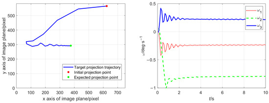
Figure 4.
The projection trajectory (left) and angular velocity (right) under the method in Ref. [39] with differential interval 0.1 s.
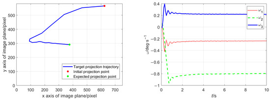
Figure 5.
The projection trajectory (left) and angular velocity (right) under the method in Ref. [39] with differential interval 0.08 s.
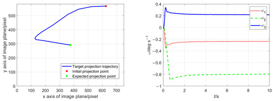
Figure 6.
The projection trajectory (left) and angular velocity (right) under the method in Ref. [39] with differential interval 0.05 s.
By comparing and observing Figure 4, Figure 5 and Figure 6 and the data in Table 7, it can be seen that for the differential control method, the time difference step has an obvious impact on the control effect. As can be seen in Figure 4, Figure 5 and Figure 6, the smaller differential steps result in a higher steady-state control accuracy and lower energy consumption. Therefore, in order to improve the control accuracy and efficiency, it is necessary to increase the frequency of the differential calculation. However, this requires higher video frame rates, more efficient image recognition algorithms, and stronger microcontrollers. Therefore, it is not a feasible approach in practice due to the performance of the onboard camera (as previously specified).
Table 7.
Comparison of three indicators with different differential time steps.
Figure 7 shows the pixel coordinate trajectory and angular velocity curve obtained by the controller designed in this paper. It can be seen that this method also achieves the adjustment of the satellite to the desired attitude. Moreover, the trajectory of the target projection (left figure) and the curve of the satellite’s angular velocity (right figure) are smoother compared with the above results corresponding to three differential time steps. There is almost no oscillation during the control process. After calculation, the indicators for this controller are and . From the perspective of attitude control stability, since is less than the results of the three differential calculations, it indicates that the deviation between the target projection point and the expected point in the stable stage is smaller. From the perspective of control efficiency, since the is also the minimum value among the four results, it indicates that the method based on visual velocity estimation consumes less energy within the same control time.
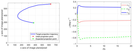
Figure 7.
The projection trajectory (left) and angular velocity (right) under the control method in this paper.
4.2.2. Impact of Measurement Noise
The process of extracting the pixel coordinates of a target from an image is accomplished by image processing techniques. The extracted pixel coordinates inevitably contain noise, and there is a certain deviation between the extracted target coordinates and the actual coordinates. For the control method of obtaining visual velocity through the differential method, the differential will also introduce noise into the visual velocity, so the effect of noise on the accuracy will be even more severe.
In this subsection, ±7 pixels of random noise were added to the actual pixel coordinates. The differential time interval was set to be 0.08 s, and the control effects of the two methods were compared under the same conditions.
Figure 8 and Figure 9 show the control effects, and Table 8 records the two indicators for the two methods. From the two figures, it can be seen that for the control method of obtaining visual velocity using differential methods, both the control torque and angular velocity curve demonstrate significant oscillations. However, for the control method proposed in this paper, the target projection trajectory and control torque are relatively smooth, with almost no oscillation.
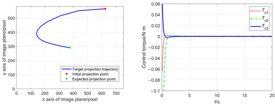
Figure 8.
Target projection trajectory (left) and control torque (right) under the control method in this paper.
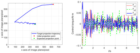
Figure 9.
Target projection trajectory (left) and control torque (right) under the control method in Ref. [39] with differential interval 0.08 s.
Table 8.
Comparison of three indicators for two controllers under noise condition.
This is because the visual velocity term plays a very important role in the control law, and the differential operation amplifies the impact of measurement noise, ultimately reflecting in the oscillation of the control torque. However, for the method designed in this paper, the visual velocity is estimated by camera parameters and is not directly affected by noise, so the image noise has a relatively smaller impact.
Comparing the values of the indicators for the two control methods in Table 8, it can also be seen that compared to the differential method, the method proposed in this paper can effectively overcome the influence of noise and achieve more stable attitude control (with the accuracy increased by about 74.53%) with lower energy consumption (reduced by about 77.47%). In addition, the peak control torque required by the method in this article is smaller than that required by the differential method, so the requirement for the maneuverability of the actuator is also lower.
5. Conclusions
To address the challenges of obtaining visual velocity and mitigating noise effects in traditional differential methods, we propose an adaptive control method based on visual velocity estimation. The estimation of visual velocity is achieved through the camera parameters, which avoids the drawbacks of time differentials. The simulation results indicate that the goal of staring control is achieved by the proposed method. Compared with the traditional differential method, the attitude accuracy is improved by about 74.53% and the energy consumption of the control process is reduced by about 77.47% under the noise condition.
The method proposed in this article is aimed at tracking and observing ground targets, whose motion is predictable due to earth rotation. However, for a large number of non-cooperative spatial targets or ground moving targets, it is difficult to obtain their motion information. Further research is needed to consider how to effectively estimate their visual velocity and track their motion without sufficient prior information.
Author Contributions
Conceptualization, C.S.; data curation, C.S. and Z.Z.; formal analysis, C.S. and C.F.; funding acquisition, C.F.; investigation, C.S.; methodology, C.S., C.F. and Z.Z.; project administration, C.F.; resources, C.F.; software, C.S.; supervision, C.F.; visualization, C.S.; writing—original draft, C.S.; writing—review and editing, C.F. and Z.Z. All authors have read and agreed to the published version of the manuscript.
Funding
This research was funded by the China Pre-Research Projects for Civil Aerospace Technology under Grant No. D030201. Funder: China National Space Administration.
Data Availability Statement
The original contributions presented in the study are included in the article, further inquiries can be directed to the corresponding author.
Conflicts of Interest
The authors declare no conflicts of interest.
References
- Lian, Y.; Gao, Y.; Zeng, G. Staring Imaging Attitude Control of Small Satellites. J. Guid. Control Dyn. 2017, 40, 1278–1285. [Google Scholar] [CrossRef]
- Zhang, X.; Xiang, J.; Zhang, Y. Tracking imaging attitude control of video satellite for cooperative space object. In Proceedings of the 2016 IEEE Advanced Information Management, Communicates, Electronic and Automation Control Conference (IMCEC), Xi’an, China, 3–5 October 2016; pp. 429–434. [Google Scholar]
- Zhang, Z.; Wang, C.; Song, J.; Xu, Y. Object Tracking Based on Satellite Videos: A Literature Review. Remote Sens. 2022, 14, 3674. [Google Scholar] [CrossRef]
- Song, C.; Fan, C.; Wang, M. Image-Based Adaptive Staring Attitude Control for Multiple Ground Targets Using a Miniaturized Video Satellite. Remote Sens. 2022, 14, 3974. [Google Scholar] [CrossRef]
- d’Angelo, P.; Máttyus, G.; Reinartz, P. Skybox image and video product evaluation. Int. J. Image Data Fusion 2016, 7, 3–18. [Google Scholar] [CrossRef]
- Julzarika, A. Utilization of LAPAN Satellite (TUBSAT, A2, and A3) in supporting Indonesia’s potential as maritime center of the world. IOP Conf. Ser. Earth Environ. Sci. 2017, 54, 012097. [Google Scholar] [CrossRef]
- Saunier, S.; Karakas, G.; Yalcin, I.; Done, F.; Mannan, R.; Albinet, C.; Goryl, P.; Kocaman, S. SkySat Data Quality Assessment within the EDAP Framework. Remote Sens. 2022, 14, 1646. [Google Scholar] [CrossRef]
- Zhang, X.; Xiang, J.; Zhang, Y. Space Object Detection in Video Satellite Images Using Motion Information. Int. J. Aerosp. Eng. 2017, 2017, 1024529. [Google Scholar] [CrossRef]
- Xiao, A.; Wang, Z.; Wang, L.; Ren, Y. Super-Resolution for “Jilin-1” Satellite Video Imagery via a Convolutional Network. Sensors 2018, 18, 1194. [Google Scholar] [CrossRef]
- He, Z.; He, D.; Mei, X.; Hu, S. Wetland Classification Based on a New Efficient Generative Adversarial Network and Jilin-1 Satellite Image. Remote Sens. 2019, 11, 2455. [Google Scholar] [CrossRef]
- Han, S.; Ahn, J.; Tahk, M.-J. Analytical Staring Attitude Control Command Generation Method for Earth Observation Satellites. J. Guid. Control Dyn. 2022, 45, 1347–1356. [Google Scholar] [CrossRef]
- Chen, X.; Ma, Y.; Geng, Y.; Wang, F.; Ye, D. Staring imaging attitude tracking control of agile small satellite. In Proceedings of the 2011 6th IEEE Conference on Industrial Electronics and Applications, Beijing, China, 21–23 June 2011; pp. 143–148. [Google Scholar]
- Wu, S.; Sun, X.; Sun, Z.; Wu, X. Sliding-mode control for staring-mode spacecraft using a disturbance observer. Proc. Inst. Mech. Eng. Part G-J. Aerosp. Eng. 2010, 224, 215–224. [Google Scholar] [CrossRef]
- Wang, J.; Liu, F.; Jiao, L.; Gao, Y.; Wang, H.; Li, L.; Chen, P.; Liu, X.; Li, S. Satellite Video Object Tracking Based on Location Prompts. IEEE Trans. Circuits Syst. Video Technol. 2024, 34, 6253–6264. [Google Scholar] [CrossRef]
- Felicetti, L.; Emami, M.R. Image-based attitude maneuvers for space debris tracking. Aerosp. Sci. Technol. 2018, 76, 58–71. [Google Scholar] [CrossRef]
- Wang, M.; Fan, C.; Song, C. Image-Based Visual Tracking Attitude Control Research on Small Video Satellites for Space Targets. In Proceedings of the 2022 IEEE International Conference on Real-time Computing and Robotics (RCAR), Guiyang, China, 17–22 July 2022; pp. 174–179. [Google Scholar]
- Pei, W. Staring Imaging Attitude Tracking Control Laws for Video Satellites Based on Image Information by Hyperbolic Tangent Fuzzy Sliding Mode Control. Comput. Intell. Neurosci. 2022, 2022, 8289934. [Google Scholar] [CrossRef]
- Zhang, X.; Xiang, J.; Zhang, Y. Error analysis of line-of-sight measurement for video satellite. Adv. Mech. Eng. 2017, 9, 168781401774282. [Google Scholar] [CrossRef]
- Wang, C.; Jiang, L.; Zhong, W.; Ren, X.; Wang, Z. Staring-imaging satellite pointing estimation based on sequential ISAR images. Chin. J. Aeronaut. 2024, 37, 261–276. [Google Scholar] [CrossRef]
- Fan, C.; Wang, M.; Song, C.; Zhong, Z.; Yang, Y. Anti-off-Target Control Method for Video Satellite Based on Potential Function. J. Syst. Eng. Electron. 2024, 35, 1583–1593. [Google Scholar] [CrossRef]
- Zhang, D.; Yang, G.; Sun, Y.; Ji, J.; Jin, M.; Liu, H. Two-phase visual servoing for capturing tumbling non-cooperative satellites with a space manipulator. Chin. J. Aeronaut. 2024, 37, 560–573. [Google Scholar] [CrossRef]
- Zhang, H.; Zhao, X.; Mei, Q.; Wang, Y.; Song, S.; Yu, F. On-orbit thermal deformation prediction for a high-resolution satellite camera. Appl. Therm. Eng. 2021, 195, 117152. [Google Scholar] [CrossRef]
- Li, L.; Zhang, G.; Jiang, Y.; Shen, X. An Improved On-Orbit Relative Radiometric Calibration Method for Agile High-Resolution Optical Remote-Sensing Satellites With Sensor Geometric Distortion. IEEE Trans. Geosci. Remote Sens. 2021, 60, 1–15. [Google Scholar] [CrossRef]
- Liang, X.; Wang, H.; Liu, Y.H.; Chen, W.; Jing, Z. Image-Based Position Control of Mobile Robots With a Completely Unknown Fixed Camera. IEEE Trans. Autom. Control 2018, 63, 3016–3023. [Google Scholar] [CrossRef]
- Kang, M.; Chen, H.; Dong, J. Adaptive visual servoing with an uncalibrated camera using extreme learning machine and Q-leaning. Neurocomputing 2020, 402, 384–394. [Google Scholar] [CrossRef]
- Xu, F.; Wang, H.; Liu, Z.; Chen, W. Adaptive Visual Servoing for an Underwater Soft Robot Considering Refraction Effects. IEEE Trans. Ind. Electron. 2020, 67, 10575–10586. [Google Scholar] [CrossRef]
- Wang, H.; Liu, Y.H.; Zhou, D. Dynamic Visual Tracking for Manipulators Using an Uncalibrated Fixed Camera. IEEE Trans. Robot. 2007, 23, 610–617. [Google Scholar] [CrossRef]
- Wang, H.; Liu, Y.H.; Zhou, D. Adaptive Visual Servoing Using Point and Line Features With an Uncalibrated Eye-in-Hand Camera. IEEE Trans. Robot. 2008, 24, 843–857. [Google Scholar] [CrossRef]
- Zhao, Z.; Wang, J.; Zhao, H. Design of A Finite-Time Adaptive Controller for Image-Based Uncalibrated Visual Servo Systems with Uncertainties in Robot and Camera Models. Sensors 2023, 23, 7133. [Google Scholar] [CrossRef]
- Jiao, J.; Li, Z.; Xia, G.; Xin, J.; Wang, G.; Chen, Y. An uncalibrated visual servo control method of manipulator for multiple peg-in-hole assembly based on projective homography. J. Frankl. Inst. 2025, 362, 107572. [Google Scholar] [CrossRef]
- Li, Z.; Lai, B.; Pan, Y. Image-Based Composite Learning Robot Visual Servoing With an Uncalibrated Eye-to-Hand Camera. IEEE/ASME Trans. Mechatron. 2024, 29, 2499–2509. [Google Scholar] [CrossRef]
- Yang, L.; Yuan, C.; Lai, G. Adaptive fault-tolerant visual control of robot manipulators using an uncalibrated camera. Nonlinear Dyn. 2023, 111, 3379–3392. [Google Scholar] [CrossRef]
- Xie, H.; Low, K.H.; He, Z. Adaptive Visual Servoing of Unmanned Aerial Vehicles in GPS-Denied Environments. IEEE/ASME Trans. Mechatron. 2017, 22, 2554–2563. [Google Scholar] [CrossRef]
- Chiang, M.-L.; Tsai, S.-H.; Huang, C.-M.; Tao, K.-T. Adaptive Visual Servoing for Obstacle Avoidance of Micro Unmanned Aerial Vehicle with Optical Flow and Switched System Model. Processes 2021, 9, 2126. [Google Scholar] [CrossRef]
- Zheng, D.; Wang, H.; Wang, J.; Zhang, X.; Chen, W. Toward Visibility Guaranteed Visual Servoing Control of Quadrotor UAVs. IEEE/ASME Trans. Mechatron. 2019, 24, 1087–1095. [Google Scholar] [CrossRef]
- Wynn, J.S. Visual Servoing for Precision Shipboard Landing of an Autonomous Multirotor Aircraft System; Brigham Young University: Provo, UT, USA, 2018. [Google Scholar]
- Zhou, J.; Wang, Q.; Zhang, Z.; Sun, X. Aircraft Carrier Pose Tracking Based on Adaptive Region in Visual Landing. Drones 2022, 6, 182. [Google Scholar] [CrossRef]
- Liu, S.; Zheng, Z.; Guan, Z.; Lin, K. Image-Based Visual Servoing Control for Automatic Carrier Landing. In Proceedings of the 2021 40th Chinese Control Conference (CCC), Shanghai, China, 26–28 July 2021; pp. 351–356. [Google Scholar]
- Song, C.; Fan, C.; Song, H.; Wang, M. Spacecraft Staring Attitude Control for Ground Targets Using an Uncalibrated Camera. Aerospace 2022, 9, 283. [Google Scholar] [CrossRef]
Disclaimer/Publisher’s Note: The statements, opinions and data contained in all publications are solely those of the individual author(s) and contributor(s) and not of MDPI and/or the editor(s). MDPI and/or the editor(s) disclaim responsibility for any injury to people or property resulting from any ideas, methods, instructions or products referred to in the content. |
© 2025 by the authors. Licensee MDPI, Basel, Switzerland. This article is an open access article distributed under the terms and conditions of the Creative Commons Attribution (CC BY) license (https://creativecommons.org/licenses/by/4.0/).