Article

Three-Dimensional Ice-Flow Recovery from Ascending–Descending DInSAR Pairs and Surface-Parallel Flow Hypothesis: A Simplified Implementation in SNAP Software

by
Alejandro Téllez-Quiñones
1,*,
Adán Salazar-Garibay
2,
Beatriz I. Cruz-Sánchez
1,
Hugo Carlos-Martínez
1,
Juan C. Valdiviezo-Navarro
1 and
Victor Soto
3
1
SECIHTI-Centro de Investigación en Ciencias de Información Geoespacial, A.C., Sierra Papacal-Chuburna Pto. Km 5, Mérida-Yucatán 97302, Mexico
2
Agencia Espacial Mexicana, Av. Insurgentes Sur 1685 Guadalupe Inn, Ciudad de-México 01020, Mexico
3
Centro de Ciencias de la Tierra, Universidad Veracruzana, Cto. Gonzalo Aguirre Beltrán SN-Zona Universitaria, Xalapa-Veracruz 91090, Mexico
*
Author to whom correspondence should be addressed.
Remote Sens. 2025, 17(7), 1168; https://doi.org/10.3390/rs17071168
Submission received: 13 January 2025 / Revised: 19 March 2025 / Accepted: 21 March 2025 / Published: 26 March 2025

Abstract

:
By considering two differential interferometric SAR signals, recovered from synthetic aperture radar (SAR) images, it has been possible to estimate the glacier velocity vector, from a method proposed by the authors Joughin, Kwok, and Fahnestock (JKF) in 1998. Although the JKF method normally works well under certain SAR observation conditions, we found a reformulated version of the main equation of this technique that may improve this interesting methodology. Thus, we present a mathematical review of this method, and a validation of our result in terms of accuracy, with some computer simulations. The innovation proposed is a simplified way to implement JKF’s work in the Sentinel Application Platform (SNAP) software, exemplified with some images from the Canadian Arctic. Generally, a north–east–up displacement estimation is considered, by using reference orthogonal coordinates, independent of the SAR image coordinates. However, we propose a methodology to estimate this velocity vector in terms of ascending or descending image coordinates. Given the importance of the JKF work, we believe that this investigation could contribute to the improvement of this technique, beyond the existence of other modern and independent methodologies.

1. Introduction

The dynamics of a glacier is based on the flow of excess ice from the accumulation zone to the ablation’s one. This flow depends on factors such as ice temperature, thickness, basal water content, and terrain slope [1]. In general, a glacier is considered in equilibrium when the volume of ice in the ablation zone is at least equal to that of the accumulation zone, ensuring its permanence over time. However, if the loss of ice during the summer exceeds that of the accumulation zone, both the thickness and surface area will retreat [2]. Unlike mountain glaciers, which are relatively small and only have tens of meters in thickness, circumpolar glaciers are much thicker and have tongues that can reach hundreds of meters or even kilometers in length [3]. The latter offers favorable conditions to analyze the glacier flow velocity of circumpolar regions, as a function of changing climatological parameters and the amount of ice accumulated over the years, through the comparison of radar satellite images.
As is well known, interferometric SAR (InSAR) and/or differential InSAR (DInSAR) techniques are widely used for monitoring topographic changes or terrain displacements induced by different phenomena, like earthquakes or seismic activity, magma accumulation due to volcanic lava flow, and particularly, glacier or ice-flow dynamics [4,5]. In the case of estimating the 3D ice-flow velocity vector v = ( v p , v q , v z ) , an interesting approach was proposed in the work of Joughin, Kwok, and Fahnestock (1998) [6] by considering at least two DInSAR signals, in ascending and descending configuration, respectively. Thus, by using the data of these interferometric pairs, and a reference digital elevation model (DEM) h = h ( p , q ) of the region of analysis, the 3D-velocity vector v = v p p + v q q + v z z , in a general orthonormal basis { p , q , z } , can be estimated from the surface-parallel flow (SPF) assumption, i.e.,
v z = h ( p , q ) · w = h p v p + h q v q ,
where h p = h / p , h q = h / q , and w : = ( v p , v q ) is the 2D horizontal velocity vector, respectively. However, the coordinates for the ascending and descending satellite data are different from the original reference coordinates where the points ( p , q , z ) are considered. Generally, p , q , z referred to east, north, and up directions, respectively. Thus, we need information on the angles induced by unitary vectors y a (ascending ground range), y d (descending ground range), and p . Specifically, α : = angle ( y a , y d ) and β : = angle ( y a , p ) , respectively (see Figure 1a). Nevertheless, if the available reference DEM h is in terms of azimuth and ground range coordinates (ascending or descending SAR satellite coordinates), we may assume without loss of generality that β = 0 , as we see later.
The basic parameters of InSAR geometry (see Figure 2a,b), as well as the reference coordinates of an ascending or a descending SAR system (see Figure 2c), are explained in Appendix A of this research. The relation between the deformation phase ϕ of a DInSAR signal, line of sight (LOS) displacement | A B | , ground range displacement d y , and vertical displacement d z (see Figure 2d), in their native ascending or descending coordinates, is also explained in this material. This information, although widely known, may be useful to understand part of the notation used in this work and how the 3D information of DInSAR data can be exploded. Particular attention must be taken into account, in the description of the moving of a point A = ( x , y , z ) to a point B = ( x + d x , y + d y , z + d z ) due to ice flow, where their respective orthogonal projections A and B onto a common azimuthal plane are displayed in Figure 2d.
Now, the organization of this research is as follows: In Section 2, velocity variables considering ascending and descending directions are described, by following the methodology exposed in reference [6], which basically consists in solving a matrix linear system of equations of order two, per each image pixel. This reference has motivated many authors to generalize the estimation of vector v , even by considering the decomposition of the LOS component in ground and azimuth directions and solving matrix systems of orders bigger than two [7]. However, we reviewed the work in [6] carefully and found a subtle detail in one of the main equations. Consequently, we propose a reformulated equation that can be applied to a general choice of possible angles between ascending and descending tracks. Apparently, this particular reformulation has not been reported in any of the many citations of Joughin, Kwok, and Fahnestock’s (JKF) paper [6], see refs [8,9,10,11,12,13,14,15,16,17], to mention a few. Thus, a modified matrix equation that matches velocity components v p and v q , in terms of deformation phases ϕ a , and ϕ d , recovered from ascending and descending data, respectively, is deduced in Section 2. Then, in Section 3, we apply our proposal to real data conformed by SAR images of the Canadian Arctic, by simplifying our velocity vector estimation in terms of the orthogonal coordinates ( p , q , z ) = ( y d , x d , z d ) , induced by the descending coordinate system with β = 0 in Figure 1b. After this reconstruction, in Section 4, we analyze the accuracy achieved with our corrected equation, in comparison to the original formula exposed in [6], by considering a simulation of ice-flow displacement. The simulation is implemented with synthetic scalar fields as the velocity components given by v , under SPF assumption, and synthetic wrapped phases (SAR interferograms) for ϕ a and ϕ d are used in order to validate our result. Finally, some points of discussion are mentioned in Section 5.

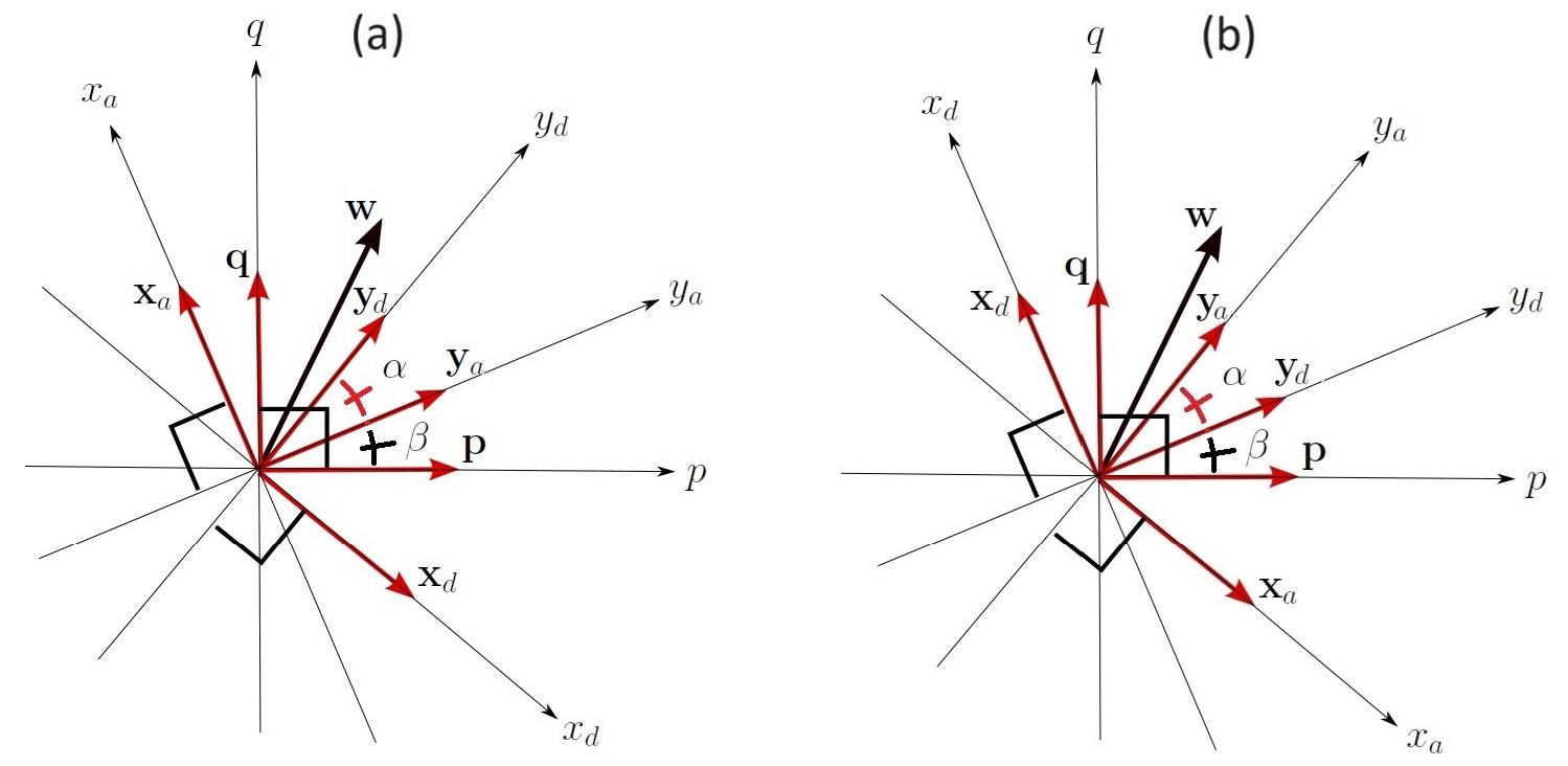
2. Horizontal Velocity Vector in Terms of Ascending and Descending Data

Since the z-components of the 3D vectors for ascending azimuth x a , ascending across track y a , descending azimuth x d , descending across track y d , p , and q are zero, they (or their projections onto plane z = 0 ) can be considered as 2D vectors similar to the horizontal velocity vector w , as depicted in Figure 1a. Now, as demonstrated in Appendix A (see Equation (A4)), the deformation phase ϕ of a DInSAR signal, recovered from a pair of images acquired at times t 1 < t 2 , is related to vertical displacement d z , and the across-track one, d y , according to the expression ϕ / ( 2 k ) = d z cos ( θ ) + d y sin ( θ ) , where θ is an observation angle. This is similar to having
σ : = ϕ 2 k Δ t sin ( θ ) v y + v z cot ( θ ) ,
by considering v z : = d z / d t , v y : = d y / d t and Δ t : = t 2 t 1 , respectively. Thus, Equation (2), rewritten as an equality, for ascending and descending deformation phases ϕ a and ϕ d , would be
σ a : = ϕ a 2 k Δ t a sin ( θ a ) = v y a + v z c a , σ d : = ϕ d 2 k Δ t d sin ( θ d ) = v y d + v z c d ,
where Δ t a = t 2 t 1 > 0 , Δ t d = t 2 t 1 > 0 , c a : = cot ( θ a ) , c d : = cot ( θ d ) , and v z = v z a = v z d , respectively. The latter is because z = z a = z d and t 1 , t 2 t 1 , t 2 , where Δ t a Δ t d (6 o 12 days, for Sentinel-1). Now, if ( v y a , v y d ) denotes the coordinates of w = ( v p , v q ) in the non-orthogonal basis { y a , y d } (with unit Euclidean norms | | y a | | = | | y d | | = 1 ), then w = v y a y a + v y d y d . Therefore, by calculating the dot product w · y a = v y a | | y a | | 2 + v y d | | y a | | | | y d | | cos ( α ) and w · y d , we find that
w · y a = v y a + v y d cos ( α ) , w · y d = v y a cos ( α ) + v y d ,
or equivalently
w · y a w · y d = 1 cos ( α ) cos ( α ) 1 v y a v y d = : B 1 v y a v y d ,
where symbol = : defines a matrix B 1 ( 2 × 2 -dimensional). Nevertheless, the system in Equation (5) in terms of inverse matrix B : = ( B 1 ) 1 is
v y a v y d = 1 sin 2 ( α ) 1 cos ( α ) cos ( α ) 1 w · y a w · y d = : B w · y a w · y d .
If we consider that p = ( p , q ) = ( 1 , 0 ) and q = ( 0 , 1 ) , it is clear from Figure 1a that y a = cos ( β ) p + sin ( β ) q and y d = cos ( α + β ) p + sin ( α + β ) q ; then, w corresponds to
v y a y a + v y d y d = cos ( β ) cos ( α + β ) sin ( β ) sin ( α + β ) v y a v y d = : A v y a v y d ,
which is the same as
w = v p v q = A σ a v z c a σ d v z c d
from Equation (3), in terms of another 2 × 2 -dimensional matrix A . Now, from the SPF assumption, Equation (8) is equivalent to writing
v p v q + ( h p v p + h q v q ) A c a c d = A σ a σ d
or
1 0 0 1 + A c a h p c a h q c d h p c d h q v p v q = A σ a σ d ,
by doing the corresponding algebraic steps. Thus, the last system is the same as
w = v p v q = ( I + A C ) 1 A σ a σ d ,
by considering
I : = 1 0 0 1 , C : = c a h p c a h q c d h p c d h q ,
respectively. On the other hand, if we substitute ( v y a , v y d ) given by Equation (6) into Equation (7), we obtain w = A B ( w · y a , w · y d ) or
w = A B v y a + v y d cos ( α ) v y d + v y a cos ( α ) = A B σ a v z c a + v y d cos ( α ) σ d v z c d + v y a cos ( α )
from Equations (3) and (4). The latter is the same as
w = A B σ a v z c a σ d v z c d + cos ( α ) A B v y d v y a ,
where the second matrix term with cos ( α ) was omitted (ambiguously) in [6], inducing a system given by w + v z A B ( c a , c d ) = A B ( σ a , σ d ) with solution
w = v p v q = ( I + A B C ) 1 A B σ a σ d ,
derived again from the same SPF assumption (see Equation (21) in [6]). In JKF’s work, matrix I + A B C in Equation (15) was reported as I A B C , because Equation (2) was taken with a switched sign, i.e., σ v y v z cot ( θ ) (see Equation (6) in [6]). Independently of this minor detail, it seems that the use of Equation (6) is unnecessary for the practical purposes of expressing w in terms of ( σ a , σ d ) . Thus, our corrected solution corresponds to Equation (11), and to the best of our knowledge, this reformulation has not been considered in any of the current works on the topic. With respect to the detail found, this is not properly an algebraic error, because the authors in [6] were conscious in their Equation (13) that
Equation (13):         v a v h T a ^ v y a w · y a = v y a + v y d cos ( α )     v d v h T d ^ v y d w · y d = v y a cos ( α ) + v y d ,
which is correct, according to our Equation (4). Nevertheless, we could have v y a = w · y a and v y d = w · y d , only when considering α = 90 [deg], and consequently (from our Equation (3)), we would be able to write
equation (12): . . . w · y a = v y a = ϕ a 2 k Δ t a sin ( θ a ) v z c a . . . w · y d = v y d = ϕ d 2 k Δ t d sin ( θ d ) v z c d
in a very similar way to what was expressed by Equation (12) in JKF’s work. Nevertheless, the correct expressions for a general angle α must be
w · y a = ϕ a 2 k Δ t a sin ( θ a ) v z cot ( θ a ) + v y d cos ( α ) , w · y d = ϕ d 2 k Δ t d sin ( θ d ) v z cot ( θ d ) + v y a cos ( α ) ,
from Equations (3) and (4), respectively. Readers can verify in JKF’s paper the detail of considering Equation (12), only valid for α = 90 [deg], in connection with Equation (14) (equivalent to our Equation (5)) and Equation (16) (equivalent to our Equation (9)), both correct in general. A review of these equations can also be conducted by considering the notation equivalences between some of the variables used in JKF’s work and the variables employed in our proposal, as displayed in Table 1.
Therefore, since JKF’s work remains an important reference point on the subject, even in research papers from the last decade (for example [18]), it is very appropriate to analyze the reformulated solution given by Equation (11).

3. Method Proposed and Real Data Experiment: Velocity Vector Estimation

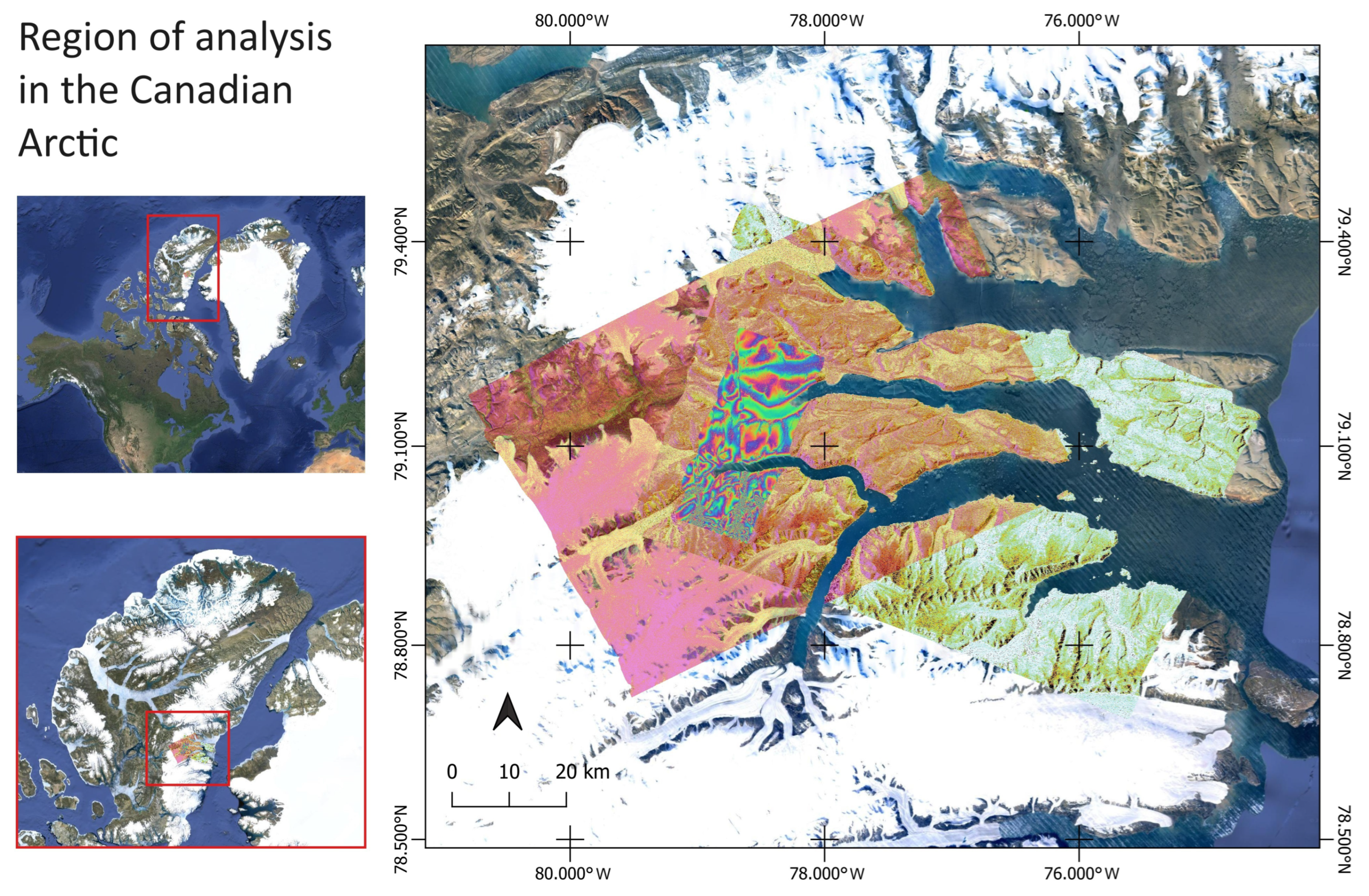
3.1. Materials and Methods
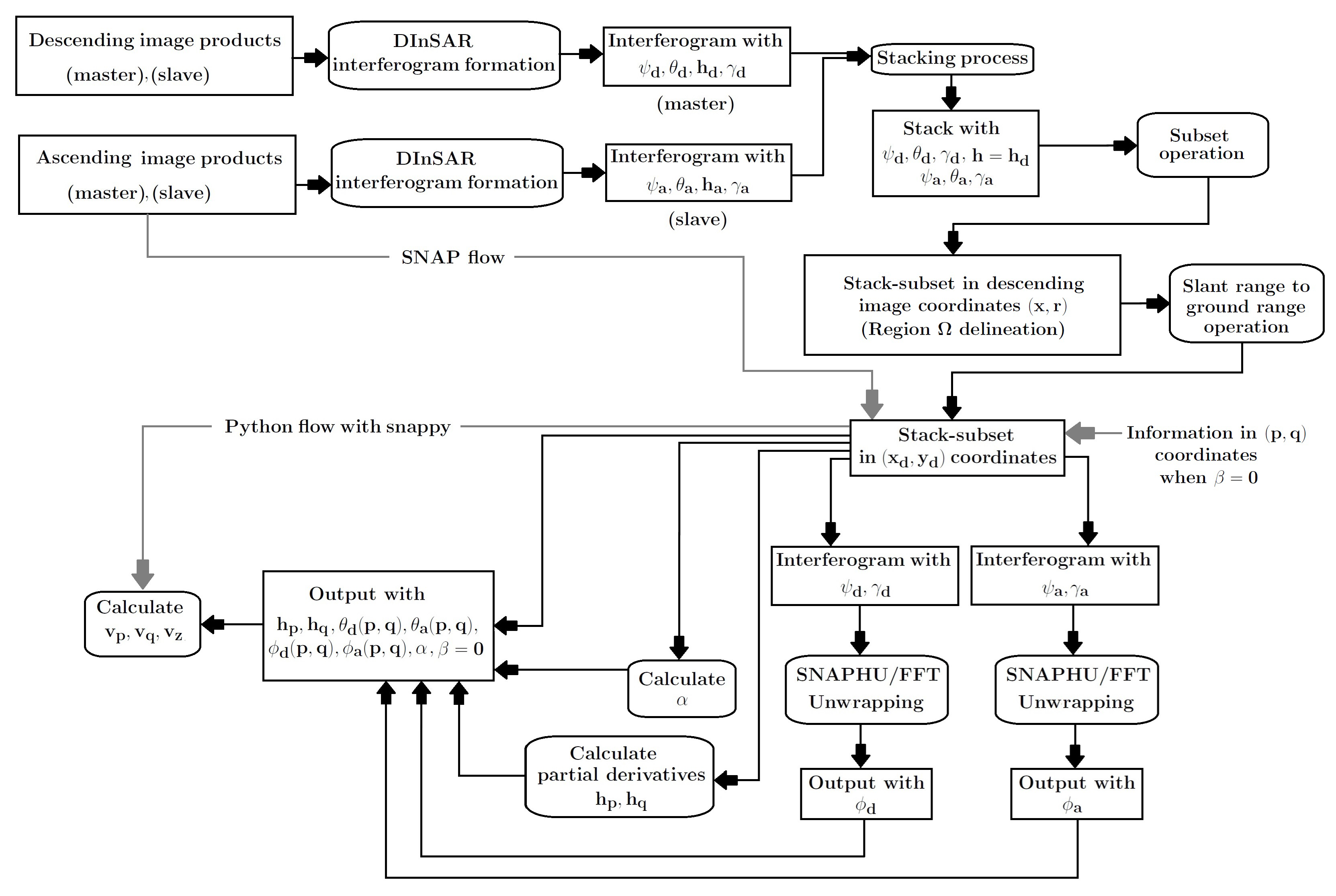
In our reconstruction, we worked with two deformation interferograms (wrapped phases ψ d and ψ a , respectively) obtained from a set of interferometric wide-swath (IW)–single-look complex (SLC) images of Sentinel-1 (SAR data with approximated wavelength λ = 0.056 [m]), with HH-polarization. To have some reference information on the phenomena under study, we downloaded some of the images of the work [18]; these images correspond to a region in the Canadian Arctic (as depicted in Figure 3), all of them acquired in February and March 2016. These interferograms were recovered from descending and ascending data, as described in Table 2.
The reason for choosing the arctic zone of Canada is because it is characterized as one of the most dynamic in terms of glacial flow velocity; that is, glaciers move with greater volume and speed per year, which is why most of the icebergs in the North Atlantic are generated by glacial flow in northeastern Canada. Although the work could have been carried out in other areas such as Antarctica, the evidence found in this work would also be noticeable, but not as clear as in this area.
The interferograms were constructed with the free software called Sentinel Application Platform (SNAP 9.0.0), according to the general steps described in [19], by considering the following preprocessing steps: S-1 TOPS Split (with the sub-swaths and bursts given in Table 2), Apply Orbit File, S1 TOPS Coregistration—S-1 Back Geocoding (with a Copernicus 30m resolution DEM [20]), Interferogram Formation, and Goldstein Phase Filtering [21]. After recovering the descending and ascending interferograms individually, we added their elevation bands (DEMs h ( x , r ) ) and saved them as non-virtual bands. Then, we added the incident angle bands θ d and θ a to each interferogram product, respectively. The latter means a conversion of the incident angle tie-point grids onto non-virtual bands, when considering the Band Maths option in SNAP. After these additions, we created a stack product of both interferograms and a subset of that stack, i.e., we followed a coregistration process (another geocoding process) of the interferograms by using the Stack-tools of SNAP (employing a bicubic interpolation method) and took a subset of the stack product. In this coregistration, the primary or master product was the descending interferogram because it was derived from the oldest image captured at Feb/29/2016. The resultant stack subset covered an area, or a possible reference domain Ω , contained in the intersection region of the two original interferometric patterns (see Figure 3).
The data arrays or bands of the stack subset were rewritten in terms of descending azimuth x : = x d and descending ground range y : = y d , by using the geometric operation Slant Range to Ground Range, available in the SNAP menu. In this way, all data such as h ( x , y ) : = h d ( x , y ) , θ d ( x , y ) , θ a ( x , y ) , ψ d ( x , y ) and ψ a ( x , y ) could be described in terms of common orthogonal coordinates ( x , y ) = ( x d , y d ) . Now, we could avoid the use of additional reference coordinates ( p , q ) in this experiment, because our reference DEM h was already given in descending coordinates ( x d , y d ) . This is similar to having p : = y d and q : = x d , which is equivalent to assuming β = 0 in Figure 1b. Therefore, points ( p , q ) = ( y d , x d ) can be defined in a reference domain Ω : = { ( p , q ) R 2 : 0 p ( N 1 ) Δ p , 0 q ( M 1 ) Δ p } . Here, Δ p : = Δ y and Δ q : = Δ x are the approximated resolution parameters of the SAR system (obtained after all the preprocessing steps), considering images of N × M -pixels. Nevertheless, we normally expressed all these scalar fields (h, θ d , θ a , ψ a , etc.) in terms of pixels ( n , m ) , through an abuse of notation, as h ( n , m ) = h ( p n , q m ) , with p n , q m = n Δ p , m Δ q and n , m = 0 , 1 , , N 1 , M 1 , correspondingly.
After the aforementioned geometric operation, we created a copy of the stack subset for implementing our own code manipulations in Python 2.7, by using the snappy library. This library can be activated by following the steps described in [22]. From this copy, we imported the interferograms ψ a and ψ d (with their corresponding coherence factors γ a and γ d ) and proceeded to unwrap these discontinuous surfaces with an appropriate unwrapping routine. By considering W as the wrapping operator [23], the unwrapping stage can be interpreted as the conversion of a DInSAR interferogram ψ = W [ ϕ ] to a phase estimate ϕ ^ = W a l g o r i t h m 1 [ ψ ] , with certain unwrapping algorithm. In SNAP software, the method used can be the statistical cost network flow algorithm for phase unwrapping (SNAPHU) [24]. Nevertheless, in the presence of unwrapping inconsistencies, we can use alternative algorithms, such as the fast Fourier transform (FFT) approach [23,25] (see the details described in Appendix B of this research).
Once the best unwrapped estimates for ϕ d and ϕ a were obtained (see Figure 4d,j), we also estimated the angle α conformed by axes y d and y a . To do this, we approximated angles θ d ( p , q ) and θ a ( p , q ) over our reference domain Ω (see Figure 4a,g), by considering fits with a global plane model of the form θ ^ ( p , q ) = c 0 + c p p + c q q , for all ( p n , q m ) Ω with n , m = 0 , 1 , , N 1 , M 1 , respectively. In this case, the estimated α corresponds to the angle induced by the gradients θ ^ d and θ ^ a , considering the corresponding fits θ ^ d and θ ^ a , where θ ^ = ( c p , c q ) and cos ( α ) = ( θ ^ d · θ ^ a ) / ( | | θ ^ d | | | | θ ^ a | | ) . All these reconstructions were carried out on an OMEN Laptop AMD Ryzen 7 4800H with 16 GB of RAM and Windows 11.

3.2. Estimated Angle α and General Processing Flow Description

After taking the subset described by region Ω , the resultant descending and ascending interferometric images had an approximated resolution parameters in descending azimuth and descending ground range coordinates, Δ q = 13.76 [m] and Δ p = 3.59 [m], with N × M = 3984 × 2415 pixels, respectively. The region Ω described by the discrete points ( p n , q m ) corresponds to a rectangle with 0 p 14.30256 [km] and 0 q 33.21664 [km], approximately. The coregistered interferograms ψ d and ψ a in terms of pixels ( n , m ) or positions ( p , q ) in region Ω are displayed in Figure 4b,h, respectively. The resolution parameters Δ q and Δ p are derived from the slant-range-to-ground-range conversion, which, according to the references in the SNAP software, consists of the following major steps: (1) create a warp polynomial of given order that maps ground range pixels to slant range pixels, (2) for each ground range pixel, compute its corresponding pixel position in the slant range image using a warp polynomial, (3) compute pixel value using the user-selected interpolation method (in our case, it was a linear interpolation).
With respect to the coregistration of the descending and ascending DInSAR interferograms (the stacking process in Figure 5), we can follow a similar description, as in the case of a single pair of SAR images; where the values of the secondary (slave) image are resampled on the common georeferenced pixels of the primary (master) image. This coregistration process can be carried out from the geocodes of both interferograms, with their corresponding restored or updated orbit files, independently of their ascending or descending geometries. The description in Section 1 and Section 2 assumes that the ascending interferogram is the primary product, while the descending one is the secondary product, i.e., an ascending–descending configuration to declare the primary–secondary interferometric products, respectively. However, Equations (3)–(12) remain valid, even if we switch the meaning of subscripts a and d in Figure 1a, i.e., subscript a for descending and d for ascending information, respectively. This means that our description in Section 1 and Section 2 could assume a descending–ascending configuration (as in our experimental case) to declare the primary–secondary interferometric products, as suggested in Figure 1b.
Now, in terms of the data for this experiment, an angle of 40 degrees between descending and ascending tracks, with equivalent supplement α = 140 [deg], was reported in the work [18]. However, the estimated α with our method was 135.01703 [deg], and according to our convention, β = 0 [deg] in our particular descending–ascending configuration.
From the unwrapped estimates ϕ d , ϕ a , the partial derivatives of our reference DEM h, the angular data θ d , θ a , and the approximated α value, we are ready to estimate de velocity components v p , v q , and v z , under the SPF hypothesis. A simplified description of our processing flow, from the reading of the image pairs to the calculation of velocity components is provided in Figure 5.

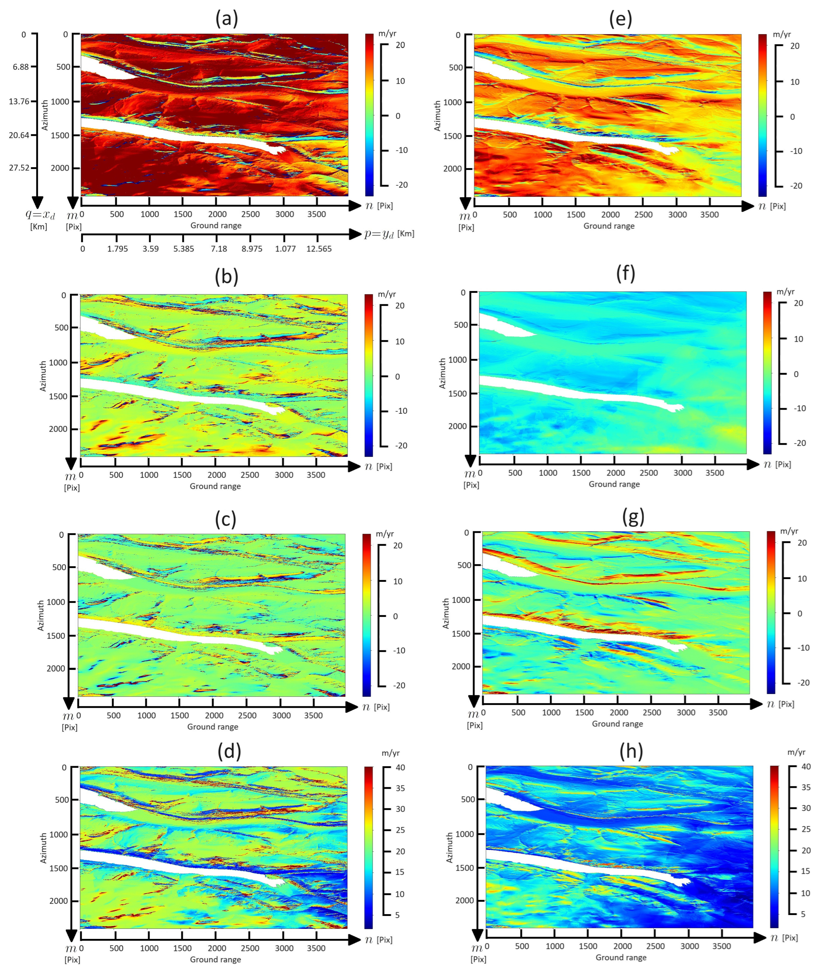
3.3. Velocity Components’ Estimation

By considering the estimated data ϕ d , ϕ a , h p , h q , α , etc., we can recover the velocity components v p , v q , and v z in two ways: through Equations (11) and (15), in order to compare or view the differences achieved from our proposed solution and the classical one, respectively (see Figure 6). It is necessary to point out that systems in Equations (11) and (15) can be quite sensitive to unwrapped phase errors because matrices ( I + A C ) and ( I + A B C ) , both dependent on DEM h-slopes, angles { α , β } , and angular distributions { θ a , θ d } , are generally ill-conditioned in some pixels ( n , m ) (as we see later). As a result, the maps for velocity components, at first glance, are badly scaled in Ω . Thus, appropriate threshold values must be considered before plotting their magnitudes.
In our case, if v p 0 (in [m/yr]) is an initial guess derived directly from Equation (15), or from Equation (11), we defined v p ( n , m ) = v p 0 ( n , m ) for pixels such that | v p 0 ( n , m ) | < T , and v p ( n , m ) = ± T (depending on the sign of v p 0 ( n , m ) ) for those pixels that exceed the magnitude of a threshold value T > 0 . Actually, different threshold values (including negative ones) as upper bounds and lower bounds can be estimated from the original data. For example, by considering the mean v ¯ p 0 and standard deviation σ p 0 of values v p 0 ( n , m ) , the upper and lower bounds can be T = v ¯ p 0 ± σ p 0 , respectively. Otherwise, we can also define the thresholds from true physical reference information when available. But in this case, we chose arbitrary upper–lower bounds T = ± 40 / 3 and applied a thresholding step with these bounds to all initial guesses v p 0 , v q 0 , v z 0 , in order to have velocity estimates v p , v q , v z , such that | | v | | = v p 2 + v q 2 + v z 2 40 [m/yr]. This means that pixel values with | | v | | = 40 have a magnitude of 40 or greater, in a similar way to how information about velocity maps in [18] is displayed.
Thus, the results obtained from Equations (11) and (15), after thresholding, are plotted in Figure 6, respectively. As we can see, these results are very different, and we could ask what improvement is achieved by the correction. Since we did not have true physical reference information (control points) of the phenomena under study, we alternatively implemented a computer simulation of ascending and descending wrapped phases in order to compare the magnitude or the percentage of error achieved from these two main equations. To see other reconstructions in a different zone of the region of analysis (see Figure 7), in a different year like 2017, we processed another set of 4 Sentinel-1 HH-polarized images, described in Table 3.
In this case, the ascending–descending configuration was considered ( p = y a , q = x a , β = 0 in Figure 1a), because the oldest image captured on 22 January 2017 was ascending. The region Ω in this new example is depicted in the ascending domain, where angle α was 135.01266 [deg]. The preprocessing steps were similar as in our previous reconstruction (by using a Copernicus 30 m DEM and FFT unwrapping); however, due to the new values for the orthogonal baselines for this new image set, the resulting resolution parameters were Δ q = Δ x a = 13.82 m and Δ p = Δ y a = 4.22 m for a delineated subset with N × M = 3011 × 2040 pixels. The ascending and the descending deformation interferograms, as well as the estimated velocity components in this new region Ω are plotted in Figure 8.

3.4. SPF Limitations and General SAR Data Details

As described in detail in [6], ice does not flow parallel to the surface, and there are many limitations and error sources to deal with, not only those properly due to the actual conditions of the region of analysis but especially those of the InSAR data. Consequently, it is very difficult to recover unambiguous measurements. According to the description in JKF’s paper, ice flow is inclined slightly upward from the surface in the ablation zone and is tipped slightly downward in the accumulation one. The authors in [6] explain that in fast-moving areas with bumpy terrain, the vertical component of motion due to SPF is large with respect to the submergence/emergence velocity. The authors also mention that in areas where there is heavy ablation or accumulation, the SPF assumption may yield significant errors in estimates of vertical motion. Nevertheless, estimates of the horizontal components of motion should be relatively unaffected by deviations from the surface-parallel flow [6]. Of course, from our new proposed equation, a possible future analysis of the capabilities and limitations of the SPF hypothesis under real situations, conducted with ground-truth data, would be very valuable. At this stage, we just could say that the limitations of this technique correspond to the same ones as for DInSAR or InSAR applications but focused on the monitoring of this specific target (snow or ice) and including precise angle estimations for α and β , between ascending and descending tracks, and the reference domain in general ( p , q ) coordinates.
For future experiments, it would be interesting to analyze other SAR data from different satellite platforms, when considering different aspects, as resolution. In our case (Sentinel-1 images), we worked with the C band, where the wavelength range was the interval [3.75 cm, 7.5 cm]. A better wavelength range for a SAR system, in terms of resolution, could be the X band, whose wavelength range is [2.5 cm, 3.75 cm] or the Ku band in the range [1.67 cm, 2.5 cm]. As is well known in the literature [26], short wavelengths permit high-resolution SAR systems and consequently, more detailed interferograms in SAR applications like this one. Normally, for InSAR or DInSAR applications, co-polarized images such as HH or VV are used, instead of cross-polarized ones such as HV or VH. This is due to the evident effects in the coherence parameter, where lower coherence values take place in DInSAR signals recovered from cross-polarized images. Low coherence values imply poor quality fringes and deficient or impossible unwrapped phase estimates. With respect to general features on the DInSAR interferogram constructions, they entirely depend on the image information, the reference DEM used in the coregistration process, and the possible additional preprocessing steps like the wrapped phase filtration. For example, the fringes recovered for the descending interferogram may look slightly different, if we add a multi-look process after the Goldstein phase filtering. The fringes would be more visible and less noisy but with lower resolution due to the sub-sampling induced by this process. In the case of the image coregistration, a low-resolution DEM (with respect to the native image resolution) makes more sense than trying to use a higher-resolution one. Of course, a higher-resolution DEM (not superior to the native image resolution) may offer a finest interferogram resolution. However, for the data in our experiment with IW-SLC images, a 30 m resolution DEM was enough. For instance, the native finest image resolution for IW-SLC products is in the range direction, which is properly a range spacing given by Δ r = 2.33 m. After a coregistration process with the Copernicus 30 m DEM in our experiment, the interferogram range resolution was Δ r = 3.57 m, and after a ground range conversion, the resulting ground range resolution was Δ y = 3.59 m, something quite acceptable.

4. Simulated Experiment: Accuracy Analysis

4.1. Synthetic Data Generation

Assuming this time the ascending–descending configuration in Figure 1a, with β = 0 [deg], our simulated interferograms ψ a = W [ ϕ a ] [rad] and ψ d = W [ ϕ d ] [rad], as functions of points ( p , q ) , could be generated by considering a rectangular domain Ω = [ 0 , p max ] × [ 0 , q max ] = [ 0 , 1495 ] × [ 0 , 2990 ] induced by a mesh of discrete points p n and q m with sampling factors Δ p = 5 [m], Δ q = 10 [m], and N = M = 300 , respectively. The angular functions θ a ( p , q ) = 0.00006 p + 29.9541 [deg] and θ d ( p , q ) = ( 0.0918 / d 0 ) [ cos ( α ) p + sin ( α ) q ] + 29.9541 [deg], where d 0 = p max 2 + q max 2 , were introduced to simulate the ascending and descending information of a hypothetical system with satellite eight H = 700000 [m] and α = angle { y a , y d } = 96 [deg] (see Figure 9a,b).
Now, the artificial DEM can be
h ( p , q ) = 500 exp ( { 4 × 10 6 [ ( p p c ) 2 + ( q q c ) 2 ] } ) [ m ]
with velocity components v p ( p , q ) = 7.5 sin [ 0.005 ( p p c ) ] [m/yr] and v q ( p , q ) = 0.005 p + 0.001 q [m/yr], where p c , q c = p max / 2 , q max / 2 [m], respectively. From the SPF hypothesis, the velocity component v z ( p , q ) [m/yr] is given by Equation (1), and, from the explicit dot products on the left in Equation (4), it can be deduced that
v p cos ( β ) + v q sin ( β ) = v y a + v y d cos ( α ) , v p cos ( α + β ) + v q sin ( α + β ) = v y a cos ( α ) + v y d ,
or equivalently that
v y a = v p [ cos ( β ) + sin ( β ) cot ( α ) ] + v q [ sin ( β ) cos ( β ) cot ( α ) ] , v y d = v p [ sin ( β ) / sin ( α ) ] + v q [ cos ( β ) / sin ( α ) ] ,
for general angles α , β . The system in Equation (21) induces a way to simulate artificial components v y a ( p , q ) , v y d ( p , q ) in terms of v p ( p , q ) , v q ( p , q ) , which in our case ( β = 0 ) would be v y a = v p v q cot ( α ) and v y d = v q / sin ( α ) . These last components can be used to declare from Equation (3) that
ϕ a = [ ( 4 π / λ ) Δ t a sin ( θ a ) ] [ v y a + v z cot ( θ a ) ] , ϕ d = [ ( 4 π / λ ) Δ t d sin ( θ d ) ] [ v y d + v z cot ( θ d ) ] ,
for all ( p , q ) = ( p n , q m ) , in terms of our synthetic data θ a , θ d , v p , v q , v z , with Δ t a = Δ t d = 0.0329 [yr] and λ = 0.056 [m].
From functions ϕ a and ϕ d , artificial SAR interferograms can be simulated by considering the addition of noise in the signal μ = cos ( ϕ ) + i sin ( ϕ ) = : c + i s , where ϕ = ϕ a , ϕ d . For example, the cosine term can be rewritten as c η ( n , m ) = c ( n , m ) + ( η / 100 ) [ 1 + 2 rand ( n , m ) ] , where 0 rand ( n , m ) 1 is a random noise distribution, and η is the percentage of noise added. In our case, we worked with signals μ η = c η + i s η with η = 15 . Thus, any noisy version of ψ a or ψ d was derived from an extended inverse tangent ψ = atan 2 [ s η , c η ] . The noisy interferograms ψ a and ψ d are shown in Figure 9c,d, and the simulated velocity components v p , v q , and v z are displayed in Figure 10a–c, respectively.

4.2. Errors Achieved by Different Ascending–Descending Across-Track Angles

Now, considering scalar fields v = v ( n , m ) as R N M vectors with Euclidean norm | | v | | , if we denote the estimations of velocity components as v ^ , where = p , q , z , we can use the normalized error 0 E [ v ^ ] = | | v v ^ | | / ( | | v | | + | | v ^ | | ) 1 (dimensionless) to analyze the accuracy of our estimations with Equations (11) and (15), after applying a thresholding step with the corresponding bounds for each synthetic, true data point v . The same normalized error formula can be used to analyze the accuracy of our unwrapped estimates, which, in this case, combine a preprocessing step consisting of applying an average filter to signal μ η , the FFT unwrapping method, and a post-processing step of congruence [23]. The resultant FFT estimates ϕ ^ = ϕ ^ a , ϕ ^ d are plotted in Figure 9e,f, where their re-wrapped versions W [ ϕ ^ ] = atan 2 [ sin ( ϕ ^ ) , cos ( ϕ ^ ) ] correspond to items (g) and (h), respectively. The normalized errors in unwrapped phases and velocity components through Equations (11) and (15) are displayed in Table 4 for α = 96 [deg] and η = 15 . As we can see, if α was close to 90 [deg], matrices ( I + A B C ) and B would be the same as ( I + A C ) and I , respectively, and good results from Equation (15) would be plausible. However, when considering α angles different from 90, such as 96, 100, or 135 (see Figure 9i–p), the accuracy of velocity estimates with Equation (15) decreased, in comparison to our correction (see Figure 10 and Figure 11, and the corresponding errors in Table 4).
As previously mentioned, velocity estimations may be quite sensitive to unwrapped phase errors and the ill-conditioning of matrices ( I + A B C ) and ( I + A C ) . That is why we plotted in Figure 10 and Figure 11 the condition number of these matrices, in natural logarithmic scale, i.e., ln ( | λ + | / | λ | ) , where | λ + | , | λ | are the module’s maximum and minimum matrix eigenvalues, respectively. To have an idea of the sensitivity of the velocity estimates with respect to the unwrapping errors, we also repeated these reconstructions with different α angles, by keeping the same velocity components but working with an increased noise factor to η = 20 , as reported in Table 5.
Clearly visible errors for the velocity estimations in the pixels of high condition number can be observed as “rings” in these particular examples (see items (h) and (l) in Figure 10 and Figure 11). Therefore, the need to consider some thresholds (information known in these simulations) is another important step for general applications with real data.
The results reported in Table 4 and Table 5 can be interpreted as follows: For α = 96 [deg], the worst normalized errors observed in Table 4 correspond to the estimates of v z ( E = 0.225 , 0.0646 ), while the worst phase estimate due to unwrapping is given by ϕ ^ d ( E = 0.0075 ). This means that for the worst error in the unwrapping stage, at about 0.75%, the worst error induced by Equation (15) is 22.5%, while with our correction, it is 6.46%.

5. Discussion and Conclusions

A mathematical review of the method proposed by Joughin, Kwok, and Fahnestock (JKF) in [6], for 3D ice-flow estimation from DInSAR data, was described. Part of our contribution in this work was the way to implement a simplified version of JKF’s method in one of the most popular free software tools: the SNAP(9.0.0) or Sentinel-1 toolbox [19] and the snappy library [22]. However, when investigating this method, a subtle detail in one of the main equations was found; specifically, Equation (15). Thus, a reformulation of this equation (given by Equation (11)), apparently unreported yet, was provided. Following this theory, a simplification of 3D ice-flow estimation in a satellite’s ascending or descending orthogonal coordinates (across-track, azimuth, and vertical directions), was also proposed, without the need to consider additional reference of a third coordinate system. This means that only information of the Sentinel-1 image captures is required.
We want to emphasize that JKF’s work has been one of the most important references on the subject since 1998; it is a very interesting approach, and a very valuable tool for the recovery of ice-flow velocity estimates from SAR data, when properly applied. Moreover, this technique could be generalized to other possible InSAR or DInSAR applications, by considering a similar hypothesis to the SPF Equation (1), which basically relates the velocity components through a linear model. Nevertheless, some references such as [27] have pointed out the accuracy differences between InSAR measurements based on the SPF hypothesis and alternative ones based on a GPS method, suggesting that the InSAR velocity estimates could be improved. Therefore, independently of the sensitivity of this technique, with respect to unwrapped phase errors, or the ill-conditioning state of the matrix ( I + A C ) for some pixels, we believe that possible improved velocity estimates could be achieved with the reformulation proposed in this research. Thus, the current reformulated equation based on the original work of [6] could be tested again, by considering reference or in situ data in some future investigations, including possible comparisons with entirely independent techniques, such as the offset tracking [28].
The errors in our computer simulations may give us an idea of the precision achieved with our correction proposed. For example, from Table 5 in the case where α = 135 [deg], we could say that for the worst error in the unwrapping stage, at about 9.82%, the worst error induced by Equation (15) was 63.66%, while with our correction it was 28.36%. However, these results are only valid when assuming the SPF hypothesis as true, i.e., this is just a preliminary work where future investigations with ground-truth data will be required. Currently, our proposal purports to improve JKF’s work on its own and not to test it or compare it with other methods. For that reason, we believe that computer simulations under the SPF hypothesis are the best way to see the improvement achieved at this stage. Our work can be considered as initial research, that eventually may be supported with more experiments applied to other regions of analysis by considering ground-truth data from open databases, such as EPOS [29].
It is important to remark that our study is a simplified version of JKF’s method, because our velocity vector estimation took place in the ascending or the descending image domain (azimuth and ground range), i.e., the region Ω . Since our current proposal is a 3D velocity estimation on the SAR image domain Ω , where the horizontal components of the flow are in azimuth and ground range directions, it would be very difficult to find an in situ reference for a validation in the same directions as those of the SAR image’s independent variables. Thus, part of our future research work is to analyze the complete and corrected JKF method, by using a third reference coordinate system (when β 0 ), where the possible in situ or reference data of the phenomena under study are available. Nevertheless, as a practical experiment in SNAP software, like those given in many of the InSAR or DInSAR application guide manuals [19], and with no more reference data, the velocity vector estimation in the ascending or descending image domain Ω may be quite useful, as preliminary monitoring.
For testing the corrected JKF approach with other methods, as well as its capabilities and limitations in complex scenarios, we may apply our new formula, by working with DInSAR signals from a fixed region of analysis, in different seasons and with many image pairs as possible, captured at closed periods. However, the simplest technique consists in using just two pairs of images (for recovering the ascending and the descending DInSAR signals) for estimating an instantaneous velocity vector. As described in reference [30], the use of at least two pairs is enough for a 3D velocity recovery. The use of more pairs in closed periods may be useful in order to expand the estimation, in a similar way to a time series analysis [31], whose main purpose would be the estimation of an average velocity vector. However, the latter is a little bit different from an instantaneous measure. The problem of estimating an instantaneous velocity vector from many pairs in closed periods is that we cannot have DInSAR signals at periods close enough. A period of 6 days is the limit for Sentinel-1, but unfortunately, the intersection of the ascending and descending tracks from that period is sometimes too small or impossible to analyze for certain regions. Subsequent estimations at closer periods may be practical to analyze the evolution or the change in the velocity vector along time and conducting at most a semi-local time analysis. But normally, when fixing a region of analysis, the availability of more than two useful Sentinel-1 image pairs for recovering a local or an instantaneous estimation is not always possible.
The implementation of the corrected JKF method would be very useful, not only to analyze its capabilities, but for future more balanced or equitable comparisons with other methods. Thus, independently of the complex factors or limitations of the SPF assumption in connection with the phenomena observed through ascending and descending DInSAR signals, the performance of this technique, at first glance, depends on the ideal conditions required for general InSAR or DInSAR applications that are not always satisfied in some cases. The absence of these conditions is translated in the common drawbacks, which we will deal with in our future analysis: low coherence in some regions of noisy or high-frequency fringes, not enough short baselines for the DInSAR data, and not enough long ones for the InSAR case, small intersections between ascending and descending tracks (where the monitoring of specific regions is not possible), imprecise angle α estimation (including β , if an additional reference coordinate system is required), bad scaling due to matrix ill-conditioning, unwrapping inconsistencies, etc.

Author Contributions

Conceptualization, methodology, software, formal analysis, and investigation and resources, A.T.-Q., A.S.-G., B.I.C.-S., and H.C.-M.; writing—review and editing, A.T.-Q., B.I.C.-S., J.C.V.-N., and V.S.; visualization and supervision, A.T.-Q., A.S.-G., H.C.-M., J.C.V.-N., and V.S.; writing—original draft preparation, A.T.-Q. All authors have read and agreed to the published version of the manuscript.

Funding

This research received no external funding.

Data Availability Statement

Part of the data of this research is shared at https://drive.google.com/drive/folders/1wT82JHCDOYF2m94ujbj3gFdsIyZYr07Z?usp=sharing (accessed on 3 March 2025).

Acknowledgments

The authors want to thank the anonymous reviewers who made possible the improvement of this work.

Conflicts of Interest

The authors declare no conflicts of interest.

Abbreviations

The following abbreviations are used in this manuscript:
SARSynthetic aperture radar
JKFJoughin, Kwok, and Fahnestock
SNAPSentinel application platform
InSARInterferometric SAR
DInSARDifferential InSAR
DEMDigital elevation model
SPFSurface-parallel flow
LOSLine of sight
IWInterferometric wide swath
SLCSingle-look complex
SNAPHUStatistical cost network flow algorithm for phase unwrapping
FFTFast Fourier transform

Appendix A. SAR Data and Its Relation with LOS Displacement

Appendix A.1. DInSAR Signals and Their Deformation Phases

If z = h 0 ( p , q ) denotes a reference DEM of the topography of a region described in an arbitrary reference orthogonal coordinate system ( p , q , z ) , where ambiguously z = 0 could be the sea level (or a tangent plane of an ellipsoid Earth model), and H > > h : = h 0 + h denotes the relation between the satellite height H (a constant) and an updated DEM h = h ( p , q ) , then the function h may approximate an ice-sheet surface, which can be recovered from an ascending pair of SAR images of a glacier region, captured at times t 0 < t 1 . The difference h can be considered as the main information recovered from an InSAR signal s = γ e i ϕ with an amplitude coherence factor γ . Here, if k = 2 π / λ is the wave number, l is the constant baseline, θ is the observation or incident angle of a point A in the terrain, and l = l cos ( θ ) is the orthogonal baseline (see Figure 2a), then
ϕ : = 2 k ( | S 1 A | | S 2 A | ) = ϕ 0 + ϕ flat + ϕ elev ,
is the interferometric phase, with well-known terms; ϕ 0 : = 2 k l sin ( θ 0 ) (reference phase), ϕ flat : = 2 k l R / [ R tan ( θ ) ] (flattening phase), and ϕ elev : = 2 k l h / [ R sin ( θ ) ] (elevation phase), respectively [32]. Thus, after a flattening Earth phase removal with the reference data ϕ flat 0 = 2 k l 0 R 0 / [ R 0 tan ( θ 0 ) ] and l 0 = l cos ( θ 0 ) , i.e., s elev : = s e i ϕ 0 e i ϕ flat 0 γ e i ϕ elev , we may estimate ϕ elev from the complex values of s elev and calculate h R 0 sin ( θ 0 ) ϕ elev / [ 2 k l 0 ] and the “current topography” h = h 0 + h (as suggested by Figure 2b). The topography h 0 to be considered may come from the SAR images’ own metadata, so h can originally depend on the ( x , r ) -image coordinates called azimuth x and zero-Doppler range r (see Figure 2c). Nevertheless, h can be rewritten as h ( x , y ) = h ( x , y ( r ) ) in orthogonal ( x , y ) coordinates, where y is called across track or ground range. Eventually, the information of h can also be rewritten as h ( p , q ) = h ( x ( p , q ) , y ( p , q ) ) in terms of other arbitrary orthogonal ( p , q ) coordinates.
From another InSAR signal s + : = γ + e i ϕ + , comprised of an ascending pair of images of the same region captured at times t 1 < t 2 , we may obtain again an interferometric phase
ϕ + ϕ topo + ϕ ,
where ϕ topo can be understood as the previous interferometric phase ( ϕ topo ϕ ), and ϕ : = 2 k | A B | is a deformation phase, which can be introduced due to an ice-flow or a terrain displacement between capture times t 1 < t 2 [32]. Thus, if we estimate ϕ from the DInSAR signal s defo : = s + e i ϕ topo γ + e i ϕ (topographic phase removal), we can approximate the LOS displacement | A B | = ϕ / [ 2 k ] , as described in Figure 2d. Since the topographic phase ϕ topo can be estimated from the previous reference DEM as h 0 + : = h , the approximated signal s defo , recovered from h 0 + and the ascending images captured in times t 1 < t 2 , would have only information of LOS displacement.
Alternatively, we may use another function h 0 + , declared as a reference DEM offered by the metadata of the primary image captured a time t 1 ; something that may not be accurate enough but reduces considerably the memory and computational cost, for practical purposes. In general, the information from another LOS displacement, by considering this time a descending pair of images of the same region (captured at times close to t 1 < t 2 ) can also be estimated. Therefore, the data recovered from these two DInSAR signals in ascending and descending configurations can be used jointly to analyze the 3D displacement of the phenomena under study, i.e., we can explode the double-view perspective of the SAR detections in different LOS directions.

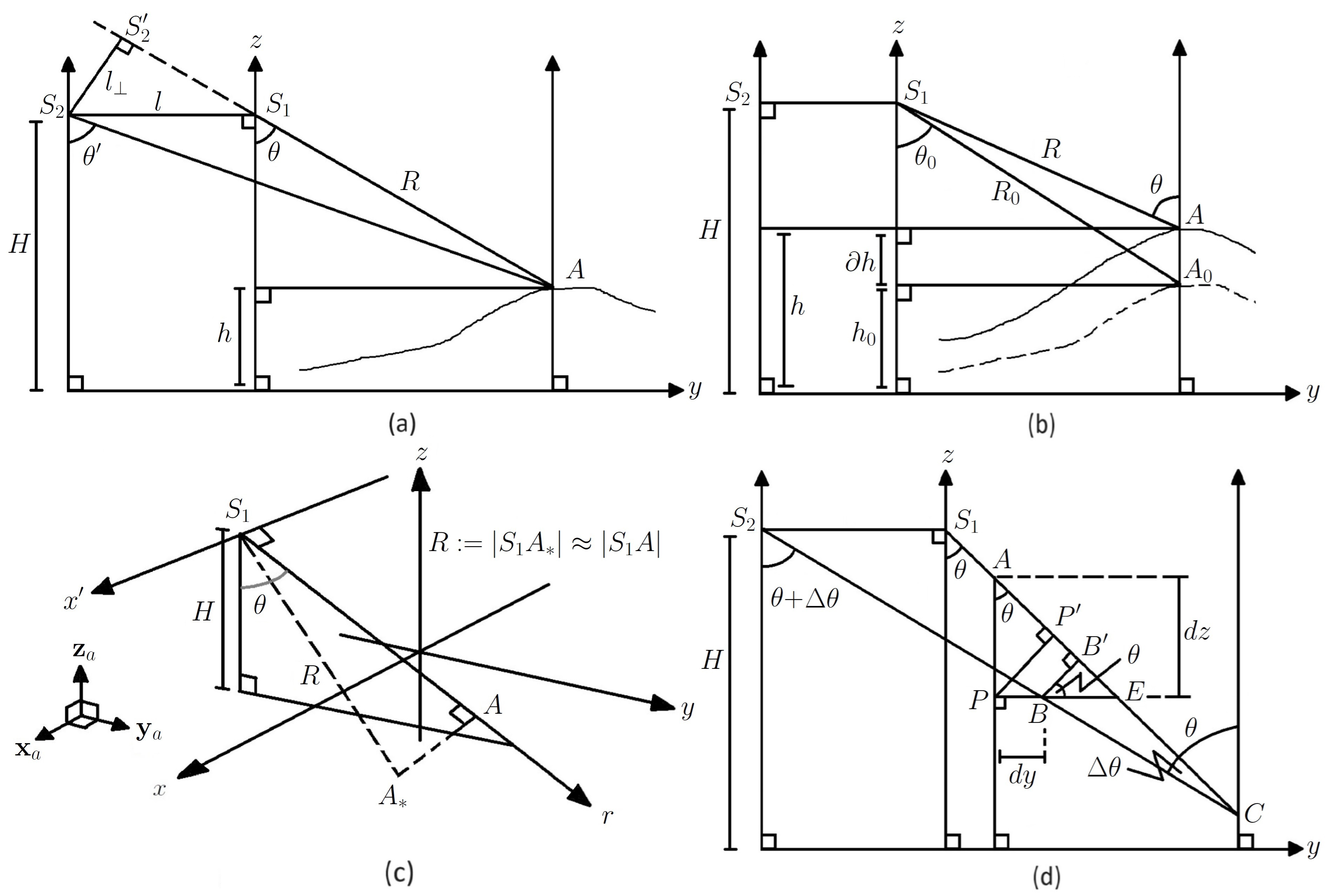
Appendix A.2. Deformation Phase and Its Relation with Ground Range and Vertical Displacements

By considering the ( x , y , z ) coordinate system of ascending (or descending) images, we can describe the displacement of a point A = ( x , y , z ) to a point B = ( x + d x , y + d y , z + d z ) due to ice flow (seismic activity, etc.). We can also consider the orthogonal projections of A and B onto a common azimuthal plane x = x 0 , given by A and B points, respectively. Then, in the plane x = x 0 (where the primary and secondary positions S 1 and S 2 are ideally located), we can approximate the vertical and the ground range displacements induced by the moving A B as the distances with sign d z ± | A P | and d y ± | P B | , as shown in Figure 2d. Here, P is just a reference point with the same height as B, located in the same vertical line as A. Thus, if visual lines | S 1 A | and | S 2 B | intersect at a point C, the information of the interferometric phase in Equation (A2) with respect to point C is ϕ + = 2 k ( | S 1 C | | S 2 C | ) , where
| S 1 C | | S 2 C | ϕ + = ( | S 1 A | | S 2 B | ) + ( | B C | | B C | ) + | A B | ( | S 1 A | | S 2 B | ) ϕ topo + | A B | ϕ .
The difference | S 1 A | | S 2 B | corresponds theoretically to the topographic phase ϕ topo (when there is no displacement, i.e., A = B = C ), and term | B C | | B C | 0 because 1 cos ( Δ θ ) = | B C | / | B C | when Δ θ 0 .
Thus, the deformation phase is basically ϕ = 2 k | A B | , where | A B | = | A P | + | P B | by considering the orthogonal projections of P and B onto line | S 1 C | , yielding P and B , respectively. However, it is easy to verify that cos ( θ ) = | A P | / | A P | and | P B | / | P B | = | B E | / | B E | = sin ( θ ) ; therefore, we have | A P | = d z cos ( θ ) and | P B | = d y sin ( θ ) . Thus, we could say that ϕ / ( 2 k ) = d z cos ( θ ) + d y sin ( θ ) , or
σ : = ϕ 2 k Δ t sin ( θ ) v y + v z cot ( θ ) ,
by declaring v z : = d z / d t , v y : = d y / d t and Δ t : = t 2 t 1 , respectively.

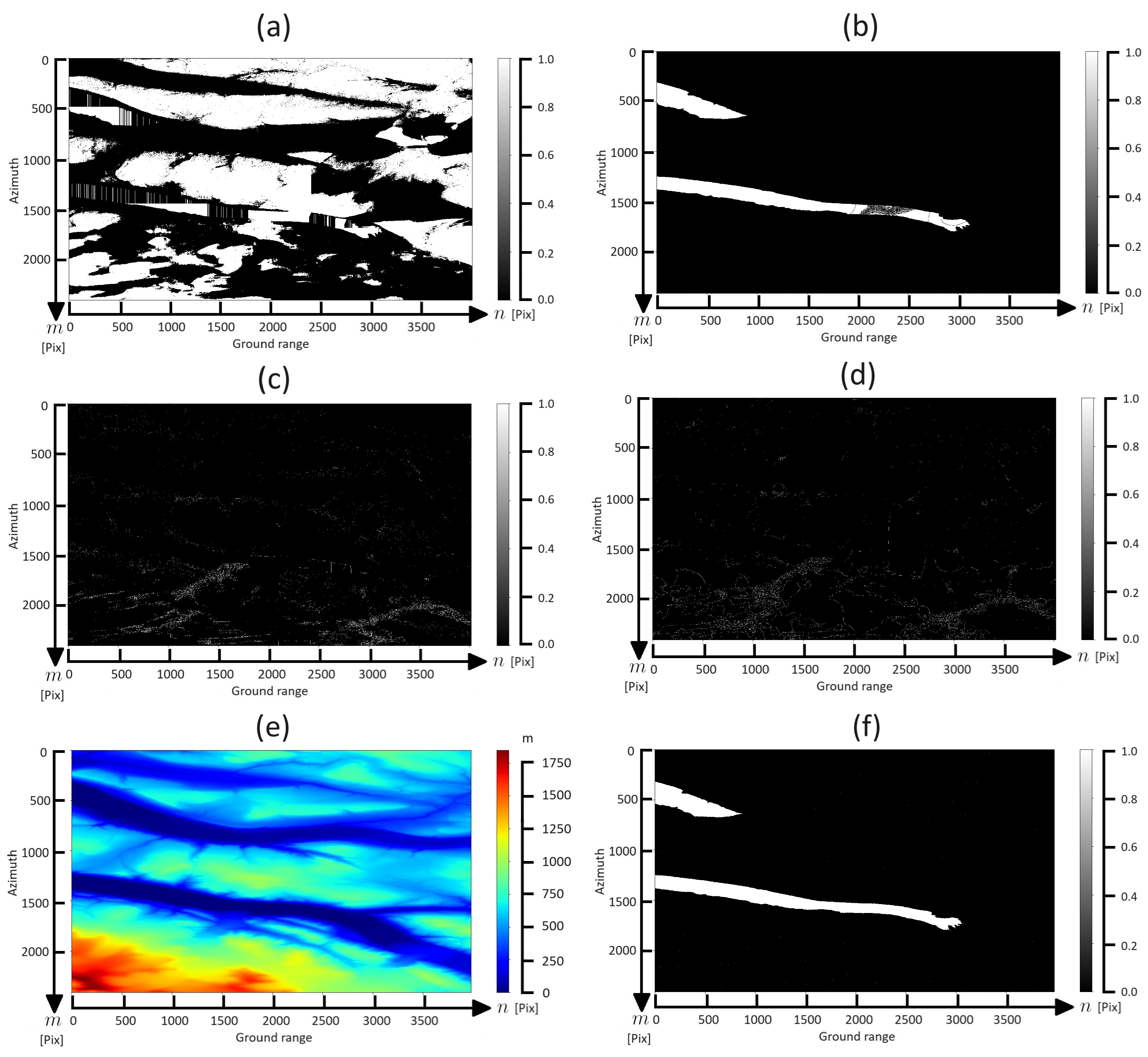
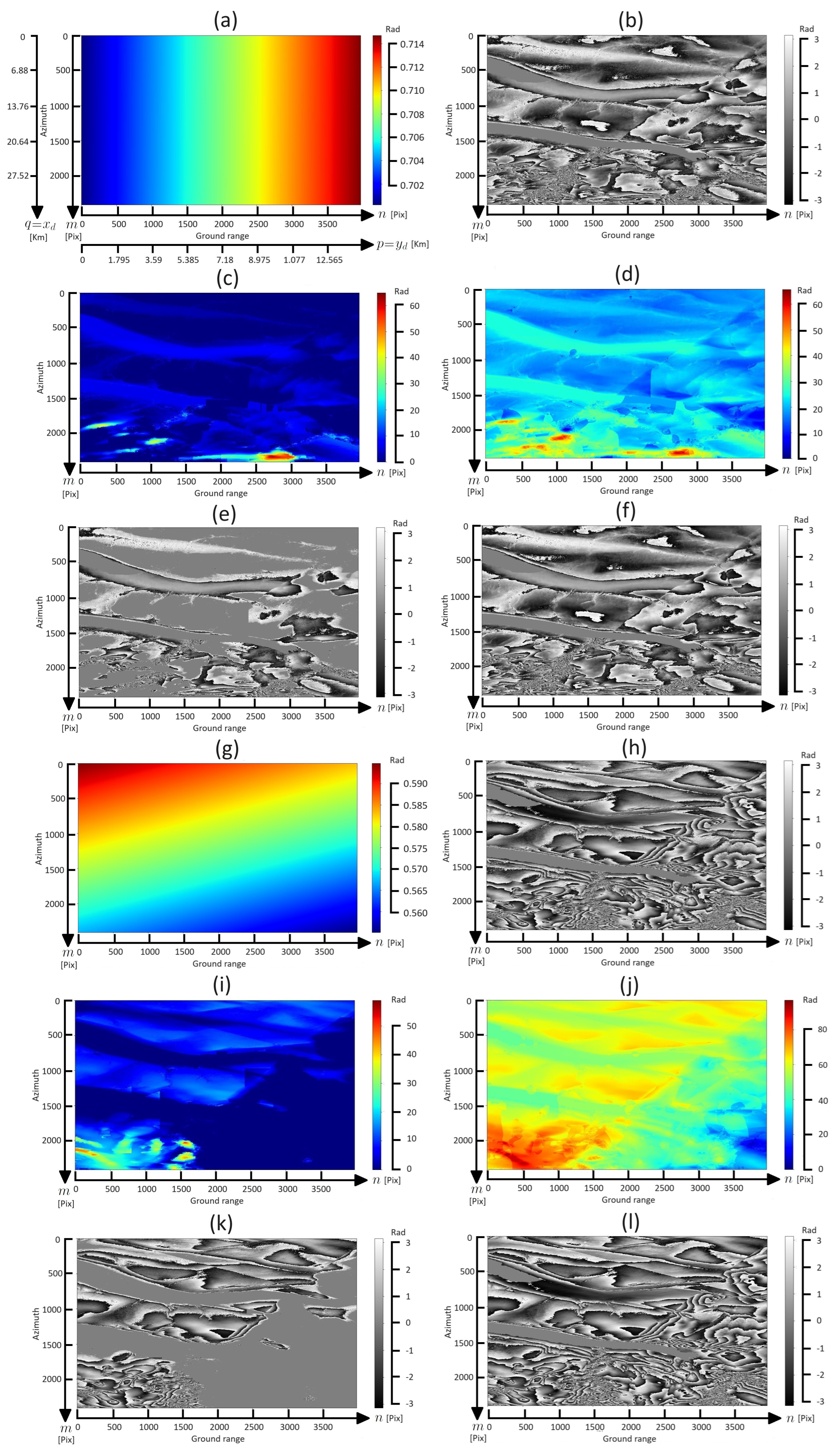
Appendix B. Results Achieved from the Unwrapping Stage

An interferogram product, derived from the stack subset with just descending data, was unwrapped by using the statistical cost-network flow algorithm for phase unwrapping (SNAPHU) [24]. From snappy code instructions applied to the stack subset, a similar interferogram product with just ascending data was created and unwrapped with the same SNAPHU algorithm. Initially, we worked with the SNAPHU algorithm, because it is the most commonly used when considering image preprocessing flow with SNAP (it is the only one available). However, as described in [32], some inconsistencies can be obtained from the SNAPHU routine, so we decided to use an additionally unwrapping method: a simple Python custom-code implementation of the fast Fourier transform (FFT)-based algorithm [23], considering an appropriate well-scaled implementation, with a simple average wrapped phase filtering and a congruence post-processing step [25].
On the other hand, the inconsistencies of the unwrapping estimates ϕ ^ = ϕ d , ϕ a for the SNAPHU and FFT algorithms can be described through binary masks with zeros (black pixels when no inconsistency is present), and ones (white pixels when an inconsistency is found). Assuming relatively smooth phase estimates, these inconsistencies are local constant regions (white pixels ( n , m ) such that i , j = 1 1 ϕ ^ ( n + i , m + j ) = 9 ϕ ^ ( n , m ) ) and Nyquist discontinuities (white pixels ( n , m ) such that | ϕ ^ ( n + 1 , m ) ϕ ^ ( n , m ) | π or | ϕ ^ ( n , m + 1 ) ϕ ^ ( n , m ) | π ), respectively. The percentage of inconsistencies with respect to the total number of pixels, for these two algorithms, was about 45.7% and 46% for descending and ascending SNAPHU estimates, respectively, and 5.9% and 5.2% for descending and ascending FFT estimates, correspondingly. As an example, the binary masks of inconsistencies observed in the descending phase estimates are plotted in Figure A1.
Figure A1. (a,b) Local constant regions for the descending phase estimate ϕ d , obtained from SNAPHU and FFT algorithms, respectively. (c,d) Nyquist discontinuities for the SNAPHU and FFT estimates, respectively. (e) Reference DEM h (measured in meters), employed in our experiment. (f) Local constant regions observed for possible water basins in h.
Remotesensing 17 01168 g0a1
It is important to remark that not all local constant regions (produced in the unwrapping stage) can be considered as inconsistencies in this case, because the phase estimate in a water body zone should be considered as zero or undefined, due to specular backscattering. Thus, after removing the pixels of local constant regions in our reference DEM h (see Figure A1e) from the local constant regions in the unwrapped phase estimations, we obtained 40.7% and 41% of inconsistencies for descending and ascending SNAPHU estimates, and 0.9% and 0.2% of inconsistencies for descending and ascending FFT estimates, respectively. As suggested by Figure A1a,b,f, it seems that the FFT result, in comparison to the SNAPHU one, correctly set the majority of these constants in the water basins. In terms of re-wrapped estimates W [ ϕ ^ ] , both methods were congruent [23], but SNAPHU result produced fewer unwrapped pixels in comparison to the FFT estimate (see Figure 4b,e,f for the descending case and Figure 4h,k,l for the ascending one).

References

  1. Hewitt, I.J.; Schoof, C. Models for polythermal ice sheets and glaciers. Cryosphere 2017, 11, 541–551. [Google Scholar] [CrossRef]
  2. Soto, V. Bedrock outcropping in the accumulation zone of the largest glacier in Mexico (Glaciar Norte of Citlaltépetl), as evidence of a possible accelerated extinction. J. Mt. Sci. 2023, 20, 338–354. [Google Scholar] [CrossRef]
  3. Cuffey, K.M.; Paterson, W.S.B. The Physics of Glaciers; Academic Press: New York, NY, USA, 2010. [Google Scholar]
  4. Goldstein, R.M.; Engelhardt, H.; Kamb, B.; Frolich, R.M. Satellite radar interferometry for monitoring ice sheet motion: Application to an Antarctic ice stream. Science 1993, 262, 1525–1530. [Google Scholar] [PubMed]
  5. Bamler, R.; Hartl, P. Synthetic aperture radar interferometry. Inverse Probl. 1998, 14, R1–R54. [Google Scholar]
  6. Joughin, I.R.; Kwok, R.; Fahnestock, M.A. Interferometric estimation of three-dimensionl ice-flow using ascending and descending passes. IEEE Trans. Geosci. Remote Sens. 1998, 36, 25–37. [Google Scholar]
  7. Shi, Y.; Liu, G.; Wang, X.; Liu, Q.; Shum, C.; Bao, J.; Mao, W. Investigating the intra-annual dynamics of Kunlun glacier in The West Kunlun Mountains, China, from ascending and descending Sentinel-1 SAR observations. IEEE J. Sel. Top. Appl. Earth Obs. Remote Sens. 2022, 15, 1272–1282. [Google Scholar]
  8. Whitehead, K.; Moorman, B.J.; Wainstein, P. Determination of variations in glacier surface movements through high resolution interferometry; Bylot Island, Canada. In Proceedings of the 2009 IEEE International Geoscience and Remote Sensing Symposium, Cape Town, South Africa, 12–17 July 2009; pp. II–230–II–233. [Google Scholar] [CrossRef]
  9. Zhou, Y.; Zhou, C.; Dongchen, E.; Wang, Z. A baseline-combination method for precise estimation of ice motion in Antarctica. IEEE Trans. Geosci. Remote Sens. 2014, 52, 5790–5797. [Google Scholar]
  10. Yang, Z.; Li, Z.; Zhu, J.; Preusse, A.; Hu, J.; Feng, G.; Yi, H.; Papst, M. An alternative method for estimating 3-D large displacements of mining areas from a single SAR amplitude pair using offset tracking. IEEE Trans. Geosci. Remote Sens. 2018, 56, 3645–3656. [Google Scholar]
  11. Kumari, S.; Ramsankaran, R.; Walker, J.P. Impact of window size in remote sensing based glacier feature tracking- a study on Chhota Shigri Glacier, Western Himalayas, India. In Proceedings of the IGARSS 2019—2019 IEEE International Geoscience and Remote Sensing Symposium, Yokohama, Japan, 28 July–2 August 2019; pp. 4175–4178. [Google Scholar] [CrossRef]
  12. Samsonov, S.; Dille, A.; Dewitte, O.; Kervyn, F.; d’Oreye, N. Satellite interferometry for mapping surface deformation time series in one, two and three dimensions: A new method illustrated on a slow-moving landslide. Eng. Geol. 2019, 266, 105471. [Google Scholar]
  13. Chang, Z.; Wang, Y.; Qian, S.; Zhu, J.; Wang, W.; Liu, X.; Yu, J. An approach for retrieving complete three-dimensional ground displacement components from two parallel-track InSAR measurements. J. Geod. 2020, 94, 1–12. [Google Scholar]
  14. Murray, K.D.; Lohman, R.B.; Kim, J.; Holt, W.E. An alternative approach for constraining 3D-displacements with InSAR, applied to a fault-bounded groundwater entrainment field in California. J. Geophys. Reseacrh: Solid Earth 2021, 126, e2020JB021137. [Google Scholar]
  15. Andersen, J.K.; Boncori, J.P.M.; Ander, K. Connectivity approach for detecting unreliable DInSAR ice velocity measurements. IEEE Trans. Geosci. Remote Sens. 2022, 60, 1–12. [Google Scholar]
  16. Ren, K.; Yao, X.; Li, R.; Zhou, Z.; Yao, C.; Jiang, S. 3D displacement and deformation mechanism of deep-seated gravitational slope deformation revealed by InSAR: A case study in Wudongde Reservoir, Jinsha River. Landslides 2022, 19, 2159–2175. [Google Scholar]
  17. Kumar, V.; Hogda, K.A.; Larsen, Y. Across-track and multi-aperture InSAR for 3-D glacier velocity estimation of the Siachen Glacier. Remote Sens. 2023, 15, 4794. [Google Scholar] [CrossRef]
  18. Sánchez-Gámez, P.; Navarro, F.J. Glacier surface velocity retrieval using D-InSAR and offset tracking techniques applied to ascending and descending passes of Sentinel-1 data for Southern Ellesmere Ice Caps, Canadian Arctic. Remote Sens. 2017, 9, 442. [Google Scholar] [CrossRef]
  19. Braun, A.; Veci, L. Sentinel-1 Toolbox: TOPS Interferometry Tutorial; ESA-SkyWatch Space Applications Inc.: Online, 2021; Available online: https://sentinel.esa.int/web/sentinel/toolboxes/sentinel-1/tutorials (accessed on 3 March 2025).
  20. Fahrland, E.; Paschko, H.; Jacob, P.; Kahabka, H. Copernicus DEM Product Handbook; AIRBUS Defence and Space: Online, 2022. [Google Scholar] [CrossRef]
  21. Goldstein, R.M.; Werner, C.L. Radar interferogram filtering for geophysical applications. Geophys. Res. Lett. 1998, 25, 4035–4038. [Google Scholar]
  22. Sharma, A. Getting Started with SNAP Toolbox in Python; Towards Data Science: Online, 2020; Available online: https://medium.com/towards-data-science/getting-started-with-snap-toolbox-in-python-89e33594fa04 (accessed on 3 March 2025).
  23. Ghiglia, D.C.; Pritt, M.D. Two-Dimensional Phase Unwrapping: Theory, Algorithms, and Software; John Wiley & Sons: Hoboken, NJ, USA, 1998. [Google Scholar]
  24. Chen, C.W.; Zebker, H.A. Two-dimensional phase unwrapping with use of statistical models for cost functions in nonlinear optimization. J. Opt. Soc. Am. A 2001, 18, 338–351. [Google Scholar]
  25. Téllez-Quiñones, A.; Chi-Couoh, D.B.; Gamboa-Salazar, L.B.; Legarda-Sáenz, R.; Valdiviezo-Navarro, J.C.; León-Rodríguez, M. Two-dimensional phase unwrapping based on Fourier transforms and the Yukawa potential spectrum. J. Opt. Soc. Am. A 2023, 40, 692–702. [Google Scholar]
  26. Hanssen, R.F. Radar Interferometry, Data Interpretation and Error Analysis; Kluwer Academic Publishers: Dordrecht, The Netherlands, 2001. [Google Scholar]
  27. Mohr, J.J.; Reeh, N.; Madsen, S.N. Three-dimensional glacial flow and surface elevation measured with radar interferometry. Nature 1998, 391, 273–276. [Google Scholar]
  28. Straozzi, T.; Luckman, A.; Murray, T.; Werner, C.L. Glacier motion estimation using offset-tracking procedures. IEEE Trans. Geosci. Remote Sens. 2002, 40, 2384–2391. [Google Scholar]
  29. Bailo, D.; Paciello, R.; Michalek, J.; Cocco, M.; Freda, C.; Jefferey, K.; Atakan, K. The EPOS multi-disciplinary Data Portal for integrated access to solid Earth science datasets. Sci Data 2023, 10, 784. [Google Scholar] [CrossRef] [PubMed]
  30. Fallourd, R.; Vernier, F.; Yan, Y.; Trouve, E.; Bolon, P.; Nicolas, J.-M. Alpine glacier 3D displacement derived from ascending and descending TerraSAR-X images on Mont-Blanc test site. In Proceedings of the 8th European Conference on Synthetic Aperture Radar, Aachen, Germany, 7–10 June 2010; pp. 1–4. [Google Scholar]
  31. Crosetto, M.; Monserrat, O.; Cuevas-González, M.; Devanthéry, N.; Crippa, B. Persistent Scatterer Interferometry: A Review. ISPRS J. Photogramm. Remote Sens. 2016, 115, 78–89. [Google Scholar] [CrossRef]
  32. Téllez-Quiñones, A.; Salazar-Garibay, A.; Valdiviezo-Navarro, J.C.; Hernandez-Lopez, F.; Silván-Cárdenas, J.L. DInSAR method applied to dual-pair interferograms with Sentinel-1 data: A study case on inconsistent unwrapping outputs. Int. J. Remote Sens. 2020, 41, 4662–4681. [Google Scholar]
Figure 1. (a) Ascending–descending configuration: Projected vectors p , q onto the Cartesian plane p q , and equivalent projected vectors x a , y a (for a primary DInSAR product in ascending pass), and x d , y d (for a secondary DInSAR product in descending pass), onto the same plane. The horizontal velocity vector is given by w , and all red vectors are unitary. Reasonable values for α (in radians) may be such that 0 < α < π . (b) Alternative descending–ascending configuration: According to the convention used for declaring the primary and secondary DInSAR products, subscripts a , d in (a) can be re-defined, i.e., a for descending (primary) and d for ascending (secondary).
Remotesensing 17 01168 g001
Figure 2. (a) Basic InSAR configuration, where points S 1 and S 2 correspond to primary and secondary satellite positions observing a common point A in the terrain. (b) Reference data R 0 , θ 0 , and A 0 with respect to a reference DEM h 0 = h 0 ( x , y ( r ) ) . (c) Reference coordinate system x y z that can be described according to an ascending pass of satellite S 1 through its orbit x , a parallel line to the x-axis with ascending azimuth direction x a and LOS given by an r-axis. (d)Vertical displacement d z and ground range displacement d y induced by the moving of point A onto B.
Remotesensing 17 01168 g002
Figure 3. Depiction of the region of analysis in the Canadian Arctic: Intensity primary images for ascending (red, left) and descending (yellow, right) tracks, considering the sub-swaths and bursts chosen in Table 2. The descending interferogram of the intersection region’s subset is also displayed. The image generation is based on World Geodetic System 1984 ensemble (EPSG:6326), which has a limited accuracy of at best 2 m. The fringe pattern in color covers the reference domain Ω in our experiment.
Remotesensing 17 01168 g003
Figure 4. Intersection region’s subset ( Ω ) analyzed as a function of pixels ( n , m ) and the orthogonal coordinates ( p , q ) = ( y d , x d ) with respect to the descending geometry: (a) incident angles θ d . (b) Descending interferogram ψ d . (c) Unwrapped estimate ϕ d recovered from the SNAPHU algorithm. (d) Unwrapped estimate ϕ d recovered from FFT routine. (e,f) Re-wrapped phases W [ ϕ d ] for SNAPHU and FFT estimates, respectively. (gl) The corresponding images to (af) for the ascending data θ a , ψ a , ϕ a , etc. Colored maps have been chosen to distinguish continuous surfaces from the discontinuous ones displayed in gray scales.
Remotesensing 17 01168 g004
Figure 5. General overview of the processing flow proposed for the implementation of JKF’s method with the SNAP software and snappy Python library, by considering β = 0 . This implementation only requires information provided from Sentinel-1 images’ own data. Our proposal can be defined using the SNAPHU algorithm by default. However, users are free to choose the best independent unwrapping routine they consider.
Remotesensing 17 01168 g005
Figure 6. (ad) Estimated velocity components v q (descending azimuth), v p (descending ground range), v z (vertical), and velocity magnitude | | v | | , recovered from Equation (15), respectively. (eh) The same estimated velocity components in (ad), recovered from our proposal in Equation (11). Velocities in the water basins for items (ah) are omitted with NaN values due to the result supported by the reference DEM h.
Remotesensing 17 01168 g006
Figure 7. Example of ascending–descending configuration with real data provided by Table 3. The ascending track is depicted in blue and the descending one in violet. The ascending interferogram for a new region Ω is displayed in rainbow colors.
Remotesensing 17 01168 g007
Figure 8. Ascending–descending experiment from data in Table 3: (a) ascending interferogram ψ a in region Ω . (bd) Velocity estimates in ascending azimuth, ground range and vertical direction, derived from Equation (15), respectively. (e) Descending interferogram ψ d in region Ω . (fh) Velocity estimates as in (bd), but derived from Equation (11), respectively. A threshold step with upper–lower bounds T = ± 25 / 3 was taking into account for all these estimates.
Remotesensing 17 01168 g008
Figure 9. (ad) Angle functions θ a , θ d , and simulated noisy interferograms ψ a , ψ d for α = 96 [deg] and noise factor η = 15 , respectively. (eh) Recovered unwrapped phases ϕ ^ a , ϕ ^ d from the FFT algorithm, and re-wrapped phases W [ ϕ ^ a ] , W [ ϕ ^ d ] , correspondingly. (ip) Equivalent items to (ah) but for α = 135 [deg] and the same noise factor.
Remotesensing 17 01168 g009
Figure 10. Experiment with α = 96 [deg] and η = 15 : (ac) Simulated velocity components v p , v q , and v z , in ascending across-track, azimuth, and vertical directions, correspondingly. (d) Angular configuration between ascending and descending systems. (eg) Resultant estimations v ^ p , v ^ q , and v ^ z , derived from Equation (15). (h) Condition number for matrix ( I + A B C ) in natural logarithmic units. (ik) Resultant estimations for the same velocity components as in (eg), but derived from Equation (11). (l) Condition number for matrix ( I + A C ) in natural logarithmic units.
Remotesensing 17 01168 g010
Figure 11. Experiment with α = 135 [deg] and η = 15 : (ac) Simulated velocity components v p , v q , and v z , in across-track, azimuth, and vertical directions, correspondingly. (d) Angular configuration between ascending and descending systems. (eg) Resultant estimations v ^ p , v ^ q , and v ^ z , derived from Equation (15). (h) Condition number for matrix ( I + A B C ) in natural logarithmic units. (ik) Resultant estimations for the same velocity components as in (eg), but derived from Equation (11). (l) Condition number for matrix ( I + A C ) in natural logarithmic units.
Remotesensing 17 01168 g011
Table 1. Notation equivalences between some of the variables of JKF’s work in [6] and the corresponding ones in our proposal (Prop.).
JKF ← Prop.JKF ← Prop.JKF ← Prop.JKF ← Prop.
v v x p y q z z
z t ( x , y ) h ( p , q ) z t x h p z t y h q v h w
a ^ y a d ^ y d v a v y a v d v y d
v x v p v y v q ϕ d , a ϕ a ϕ d , d ϕ d
ψ a θ a ψ d θ d δ T a Δ t a δ T d Δ t d
α , β α , β A A B B C C
Table 2. IW-SLC products used to generate the deformation interferograms ψ d and ψ a to be processed. Both interferograms represent LOS displacements per intervals of revisit Δ t d = Δ t a 0.0329 years (12 days).
InterferogramAcquisition DateBaseline l Sub-Swath and Bursts
ψ d 29/Feb/2016 (descending)30.7 [m]IW2-Bursts 7-8-9
12/Mar/2016 (descending)
ψ a 04/Mar/2016 (ascending)47.06 [m]IW1-Bursts 4-5-6
16/Mar/2016 (ascending)
Table 3. IW-SLC products used to generate deformation interferograms ψ a and ψ d from images of the Canadian Arctic in 2017.
InterferogramAcquisition DateBaseline l Sub-Swath and Bursts
ψ a 22/Jan/2017 (ascending)16.84 [m]IW1-Bursts 4-5-6
03/Feb/2017 (ascending)
ψ d 30/Jan/2017 (descending)92.56 [m]IW2-Bursts 7-8-9
11/Feb/2017 (descending)
Table 4. Normalized errors in velocity estimates E [ v ^ ] ( = p , q , z ) and in unwrapped phases E [ ϕ ^ ] ( ϕ ^ = ϕ ^ a , ϕ ^ d ), for different angles α [deg], Equations (11) and (15), and a noise factor η = 15 .
α Equation E [ v ^ p ] E [ v ^ q ] E [ v ^ z ] E [ ϕ ^ a ] E [ ϕ ^ d ]
96Equation (15)0.15180.11610.22500.00470.0075
Equation (11)0.04240.03230.0646
100Equation (15)0.20270.15570.29800.00730.0045
Equation (11)0.03560.02740.0562
135Equation (15)0.47410.30980.59810.00760.0039
Equation (11)0.02590.02520.0597
Table 5. Normalized errors in velocity estimates E [ v ^ ] ( = p , q , z ) and in unwrapped phases E [ ϕ ^ ] ( ϕ ^ = ϕ ^ a , ϕ ^ d ), for different angles α [deg], Equations (11) and (15), and a noise factor η = 20 .
α Equation E [ v ^ p ] E [ v ^ q ] E [ v ^ z ] E [ ϕ ^ a ] E [ ϕ ^ d ]
96Equation (15)0.13110.11230.21250.04250.0116
Equation (11)0.09130.06640.1296
100Equation (15)0.30790.19180.41680.13210.0252
Equation (11)0.20970.12890.2956
135Equation (15)0.52280.31990.63660.09820.0067
Equation (11)0.17250.11290.2835
Disclaimer/Publisher’s Note: The statements, opinions and data contained in all publications are solely those of the individual author(s) and contributor(s) and not of MDPI and/or the editor(s). MDPI and/or the editor(s) disclaim responsibility for any injury to people or property resulting from any ideas, methods, instructions or products referred to in the content.

