Deep Learning Methods for Inferring Industrial CO₂ Hotspots from Co-Emitted NO₂ Plumes

Abstract

The “top-down” global stocktake (GST) requires the processing of vast volumes of hyperspectral data to derive emission information, placing greater demands on data processing efficiency. Deep learning, leveraging its strengths in the automated and rapid analysis of image datasets, holds significant potential to enhance the efficiency and effectiveness of data processing in the GST. This paper develops a method for detecting carbon dioxide (CO₂) emission hotspots using a convolutional neural network (CNN) with short-lived and co-emitted nitrogen dioxide (NO₂) as a proxy. To address the data gaps in model parameter training, we constructed a dataset comprising over 210,000 samples of NO₂ plumes and emissions based on atmospheric dispersion models. The trained model performed well on the test set, with most samples achieving an identification accuracy above 80% and more than half exceeding 94%. The trained model was also applied to the NO₂ column data from the TROPOspheric Monitoring Instrument (TROPOMI) for hotspot detection, and the detections were compared with the MEIC inventory. The results demonstrate that in high-emission areas, the proposed method successfully identifies emission hotspots with an average accuracy of over 80%, showing a high degree of consistency with the emission inventory. In areas with multiple observations from TROPOMI, we observed a high degree of consistency between high NO₂ emission areas and high CO₂ emission areas from the Global Open-Source Data Inventory for Anthropogenic CO₂ (ODIAC), indicating that high NO₂ emission hotspots can also indicate CO₂ emission hotspots. In the future, as hyperspectral and high spatial resolution remote sensing data for CO₂ and NO₂ continue to grow, our methods will play an increasingly important role in global data preprocessing and global emission estimation.

1. Introduction

The Paris Agreement signed by 194 countries and the European Union committed to limiting the increase in global average temperature to below 2 °C above pre-industrial levels by 2100 to combat the dangers of global warming [1]. Compiling greenhouse gas emission inventories is a fundamental task in addressing global warming. Through these inventories, we can identify the main sources of greenhouse gas emissions, assess regional emission statuses, and estimate future mitigation potential, thereby aiding the formulation of relevant emission reduction policies [2,3]. CO₂ is the most significant greenhouse gas, accounting for approximately 72% of total anthropogenic greenhouse gas emissions [4]. Currently, there are two main methods for estimating CO₂ emissions: “bottom-up” statistical methods and “top-down” retrieval methods based on observed CO₂ data [5]. The “top-down” method offers advantages in terms of inventory timeliness, result transparency, and global comparability, making it an internationally recognized approach for carbon verification [6,7]. However, a major challenge with the “top-down” method is distinguishing between natural and anthropogenic CO₂ emissions [8,9,10], which makes the accurate determination of anthropogenic emissions difficult.

Industrial activities are the primary source of anthropogenic CO₂ emissions, accounting for more than 70% of global CO₂ emissions. Therefore, quantifying industrial emissions is a key step in estimating anthropogenic emissions. Point sources are a typical feature of industrial emissions, such as thermal power plants and steel mills, accounting for more than 40% of global annual anthropogenic CO₂ emissions [11,12]. Due to its long lifetime, CO₂ can remain in the atmosphere for extended periods, undergoing global transport and mixing [13,14]. As a result, atmospheric CO₂ exhibits higher background concentrations and smaller gradient variations. This requires extremely high-precision observations to distinguish CO₂ concentration changes ($\Delta$CO₂) and enable accurate emission retrieval [15].

Currently, satellites dedicated to the remote sensing of CO₂ include GOSAT-1/2, Gaofen-5, Tansat, and OCO-2 [16,17]. However, these satellites primarily observe in a point or strip pattern, with spatial resolutions greater than 1 km, observation intervals exceeding 200 km, and retrieval accuracies of approximately 1–4 ppm [18]. These satellites are suitable for climate research, offering spatial resolutions in the order of hundreds of kilometers and temporal resolutions at the scale of months. However, their coarse spatial resolution and distinct observation methods limit their suitability for point-source monitoring, as they struggle to detect subtle $\Delta$XCO₂ and have insufficient observation coverage. In 2019, OCO-3 was successfully launched on the International Space Station (ISS). Similar to OCO-2, OCO-3 features an additional 2-axis pointing mirror assembly (PMA) that can be observed in the Snapshot Area Map (SAM) mode. This upgrade allows for the observation of larger areas (80 km × 80 km), compensating for the narrow observation range of previous carbon monitoring satellites and enabling selective monitoring of high-emission power plants during transit [19,20]. However, OCO-3 still has a relatively coarse spatial resolution (about 1.3 × 2.3 km²), which results in spatial averaging effects on concentration measurements. Furthermore, CO₂ concentration changes are influenced by various factors, including transportation, residential areas, and vegetation [21,22]. Therefore, accurately estimating industrial CO₂ emissions and eliminating other influencing factors using the “top-down” method based on observed CO₂ concentration data remain challenging.

CO₂ and NO₂ are co-emitted during the high-temperature combustion of fossil fuels [23]. Compared to CO₂, the background concentration of NO₂ in the atmosphere is relatively low, and anthropogenic emissions, such as those from industrial activities, create a distinct contrast with this background. Additionally, NO₂ has active chemical properties and a relatively short lifetime—typically just a few hours—resulting in local concentration clustering. This clustering behavior provides a direct indication of anthropogenic emissions. Lei identified the spatial correlation between the NO₂ and CO₂ concentration increments from TROPOMI by reconstructing the concentration field using the WRF-Chem model [24]. Based on the ${\mathrm{NO}}_X$/CO₂ ratio, Yang indirectly estimated daily CO₂ emissions from fossil fuel sources using TROPOMI’s NO₂ data [25]. In terms of satellite-based NO₂ emission source identification, Finch developed an algorithm that uses TROPOMI’s NO₂ data fields to automatically detect emission plumes and infer anthropogenic combustion emissions, achieving the accurate location identification of hotspot emissions [26]. The proposed method is based on a deep learning model, and the initial training data are provided by manual interpretation. However, manual plume identification is subjective, inaccurate, and time-consuming. More importantly, this approach yields qualitative results (i.e., identifying the presence or absence of NO₂ plumes). Building on previous research, we advanced this work by not only determining the location of emission sources but also quantifying the emissions. By incorporating atmospheric dispersion models, we took a significant step forward in estimating NO₂ emissions using deep learning.

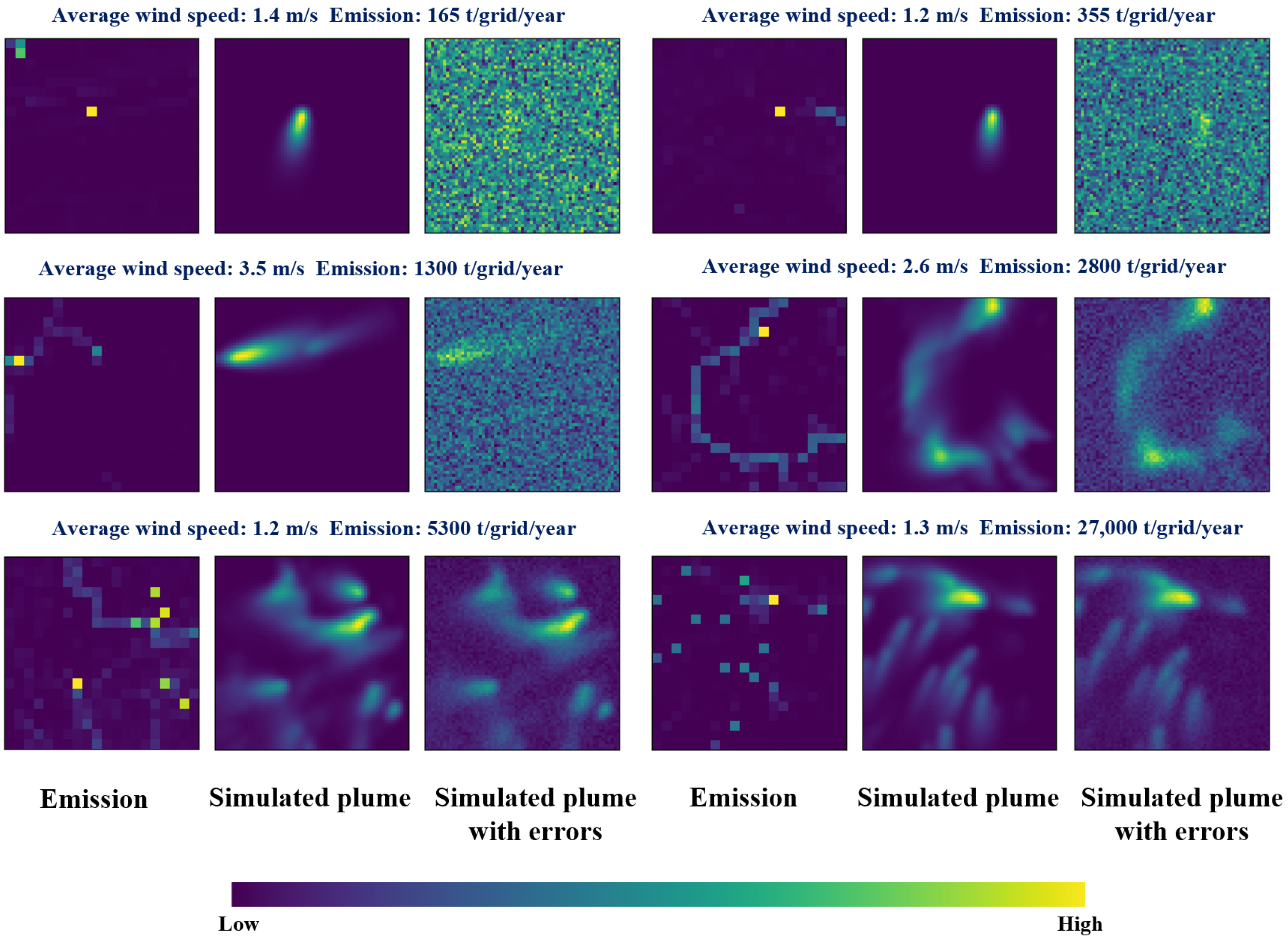
In this study, atmospheric dispersion models were used to simulate NO₂ plume-emission scenarios. This not only increases the number of training datasets but also enhances the reliability of model training and enables the trained model to quantitatively detect emissions. A convolutional neural network (CNN) model was constructed to identify NO₂ emission sources from the simulated data. The model was then applied to TROPOMI data to identify NO₂ emission sources. Finally, the co-emission of NO₂ and CO₂ in industrial emissions was leveraged to locate anthropogenic CO₂ emissions, and the detection results were compared and analyzed with existing inventories.

2. Training Dataset

2.1. NO₂ Plume Simulation

Datasets are crucial for training model parameters. However, existing research currently faces a shortage of adequate training data. Due to the chemically reactive nature of atmospheric NO₂, with a lifetime of only a few hours, it is often modeled using an empirical Gaussian plume approach [27]. Given our focus on satellite observations, we adopted a vertically integrated Gaussian plume model for NO₂, which simulates the NO₂ column concentrations observed by satellites like TROPOMI. The model formula is as follows:

$$G(x,y)={\displaystyle \frac{QH\left(x\right)}{\sqrt{2\pi }u\sigma \left(x\right)}}exp\left(-{\displaystyle \frac{y^2}{2\sigma {\left(x\right)}^2}}\right)+V_{\mathrm{bg}}(x,y)$$

(1)

where Q is the NO₂ emission rate, u is the wind speed, and $V_{\mathrm{bg}}(x,y)$ represents the background column concentration. $H\left(x\right)$ is the Heaviside step function, with coordinates x and y denoting the directions along and across the plume, respectively. And the coordinates x, y are along and across the plume direction. The diffusion width across the plume direction is given by Equation (2).

$$\sigma \left(x\right)=\sqrt{{\displaystyle \frac{2K{x}^{\kappa }}{u}}}$$

(2)

where K is the eddy diffusion coefficient in ${\mathrm{m}}^2/\mathrm{s}$, representing potential variations in the diffusion rate along the plume, depending on meteorological conditions.

For short-lived NO₂, Equation (1) must include an attenuation term.

$$D(x,\tau )=H\left(x\right)exp\left(-{\displaystyle \frac{x}{u\tau }}\right)$$

(3)

where $\tau$ represents the lifetime of the gas, approximately 4 h for NO₂.

To adapt the single-point-source model for multi-point-source simulation, we modified this model using the following steps: (1) unifying the coordinate systems; (2) rotating and translating the simulation results of the single-point source; and (3) superimposing the simulation results from multiple point sources.

2.2. Simulation Parameter Selection

To simulate realistic NO₂ plumes, we used “true” parameters. NO₂ emission is sourced from the Emissions Database for Global Atmospheric Research (EDGAR), while wind field data is obtained from ECMWF Reanalysis v5 (ERA5) meteorological reanalysis data [28]. EDGAR provides gridded data with a spatial resolution of 0.1° × 0.1° and a temporal resolution of months. EDGAR estimates NO₂ emissions following IPCC guidelines, ensuring the results are both reliable and comparable with those reported by European member states and the UNFCCC. ERA5 meteorological data provide three-dimensional atmospheric wind reanalysis from the 1940s, with a spatial resolution of 0.25° × 0.25°, and are widely recognized globally. We transformed these data from a geographic coordinate system (in degrees) to a projected coordinate system (in meters). To ensure consistency with the spatial resolution of TROPOMI NO₂ data (3.5 × 7 km²) [29], we randomly sampled both the emission and corresponding wind field data at a 4 km spatial resolution within a 64 × 64 pixel grid, covering a total area of 256 × 256 km².

2.3. Background Noise

The TROPOMI NO₂ data contain uncertainties arising from instrument and retrieval errors, necessitating the addition of noise to the simulated plume image to replicate the concentration observed by the instrument [30,31]. Common noise types include uniform noise, salt-and-pepper noise, and Gaussian noise. Uniform noise is randomly and evenly distributed within a specific range, with a mean value close to zero. Salt-and-pepper noise, also known as impulse noise, is characterized by random occurrences of white or black spots, typically caused by sudden strong interference or analog-to-digital conversion errors. In contrast, Gaussian noise follows a probability density function consistent with a normal distribution (Gaussian distribution) and has a well-defined mathematical expression. In satellite remote sensing, many types of noise can be approximated using Gaussian noise. Therefore, Gaussian noise was chosen to construct the “real” noise in this study. The range of the mean and variance of the normal distribution was determined through statistical analysis of TROPOMI concentration field data.

Taking the China as an example, we acquired emission and wind field data from EDGAR and ERA5 for the entire country. We randomly selected emission and corresponding wind field data at a spatial resolution of 4 km. These data were then modeled using a plume model with random noise added. Figure 1 illustrates the NO₂ plume shapes for different emission levels, as well as the plume shapes after adding noise. As shown in the figure, when emissions are less than 350 tons/grid/year, the NO₂ enhancement caused by the emissions is easily overshadowed by background noise, making the concentration increment nearly undetectable. At emission levels of around 1000 tons/grid/year, the NO₂ concentration increment becomes detectable, although it remains influenced by background noise. When emissions exceed 5000 tons/grid/year, the concentration increment is significantly higher than the background noise, resulting in a more distinct plume shape.

3. CNN Networks Incorporating Spatial Neighborhood Information

A convolutional neural network (CNN) is a multi-layer network with a large number of parameters, capable of extracting effective features from input image data and establishing complex relationships. CNNs have broad application prospects in fields such as remote sensing and computer vision. The convolutional neural network (CNN) model in specific applications relies on the configuration of network parameters, which need to be optimized using a training dataset. Through the backpropagation mechanism, these parameters are iteratively adjusted to achieve an optimal configuration. In addition to data, a CNN model requires a foundational network structure. Several classic network architectures, such as U-net, have been developed. For example, Bruno had utilized U-net for CH₄ plume detection and emission estimation, highlighting the strong potential of deep learning in CH₄ identification and analysis [32]. However, as the depth of CNN models increases, issues such as vanishing gradients become more pronounced during training, affecting the model’s convergence. To address this issue, researchers have adopted residual neural networks (ResNet) [33]. ResNet introduces residual modules and connections, which not only enhance the accuracy and generalization ability of deep neural networks but also mitigate vanishing and exploding gradient problems, thereby accelerating network convergence.

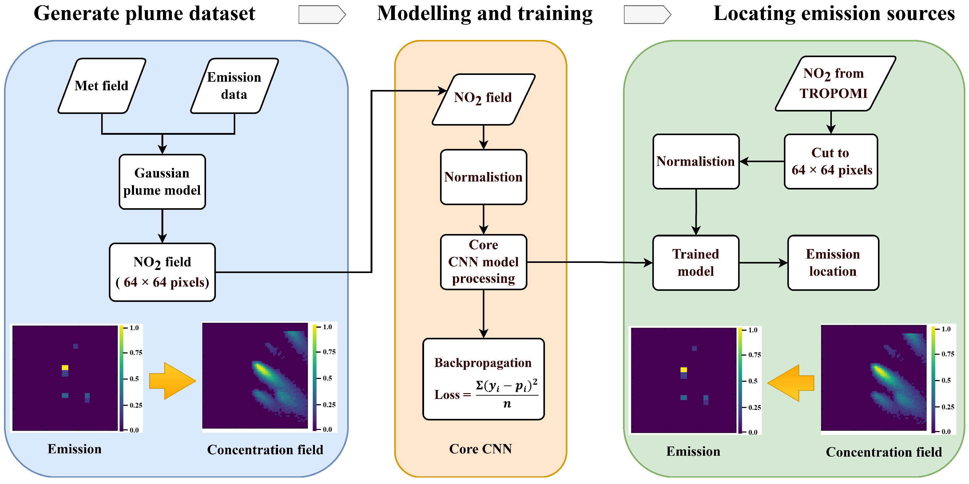
The location of anthropogenic CO₂ emission sources can be inferred using NO₂ data. The process of identifying emission hotspots is illustrated in Figure 2. First, meteorological and emission data were used to simulate a large number of NO₂ plumes. Next, a convolutional neural network (CNN)-based model was constructed, using the simulated plume-emission data as training input to enable learning. Finally, the trained model was applied to TROPOMI observational data to identify emission hotspots.

3.1. Core Network Structure

CNNs can extract pattern information such as edges, textures, and gradient changes in data through convolution operations, making them highly suitable for capturing spatial distribution characteristics in hotspot recognition. This is the primary reason we chose a CNN as the foundation for network design. Additionally, ResNet introduces residual connections, which facilitate better gradient propagation during training and enhance network performance. This is demonstrated as follows:

$$y=F\left(x\right)+x$$

(4)

where y represents the output of the residual block, and x is the input of the residual block added via the shortcut connection.

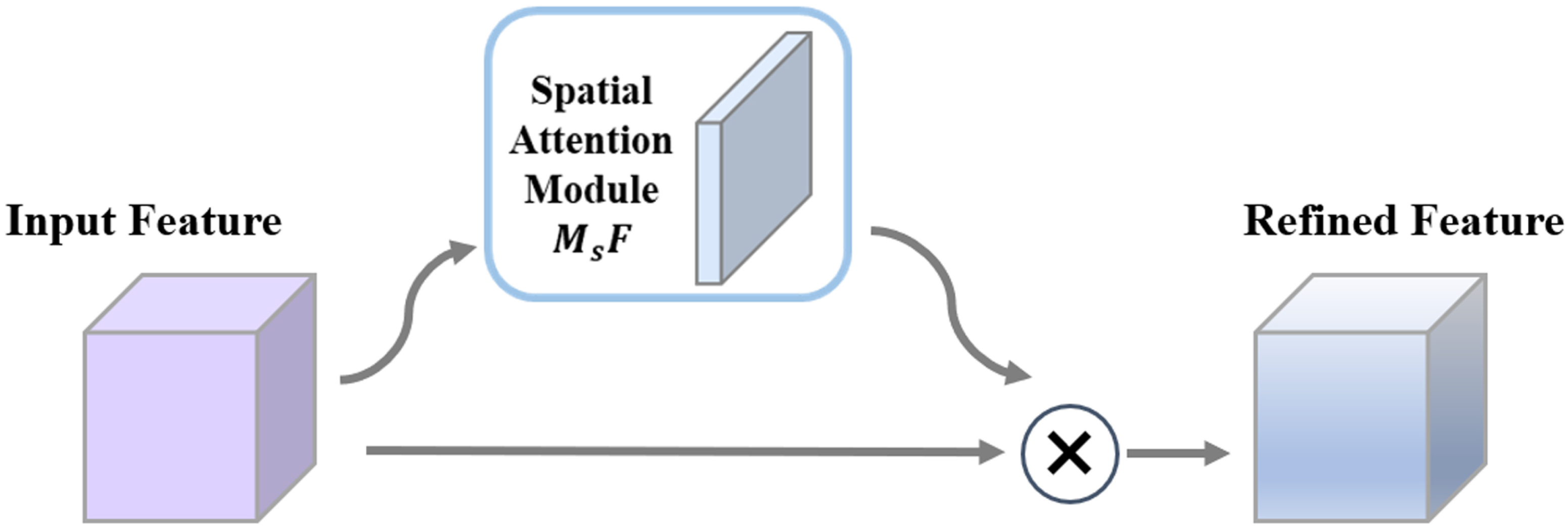
Figure 3 shows the network structure we designed, comprising an input layer, a spatial attention module, a residual neural network block, and an output layer. The spatial attention module identifies effective regions for spatial feature extraction and facilitates the fusion of spatial features from the input data. The 2D convolution (Conv) operations in the figure employ a kernel size of 3 × 3. Additionally, batch normalization (Batch Normalization) and max pooling (MaxPooling2D) are incorporated into each module, though they are not explicitly depicted here. The model’s final output is flattened and passed through a fully connected layer.

The essence of spatial attention is to extract the location information of interest within the network while suppressing invalid information. Assuming the initial input corresponds to the NO₂ concentration field data, representing the spatial dimension, the activation function ultimately generates spatial attention by accepting the output from the spatial attention module, as shown in Figure 4. Its mathematical expression is:

$$F^{*}=F\otimes \sigma M_{S}F$$

(5)

where ⊗ represents the spatial product operator, $\sigma$ denotes the activation function, and $M_{S}F$ signifies the spatial attention map.

3.2. Normalization and Loss Function

As shown in Figure 2, the designed model can be used to identify emissions based on concentration data. However, in practice, Gaussian diffusion simulations introduce biases, and discrepancies exist between the simulated and actual plumes. Accurately estimating these deviations requires a more advanced atmospheric transport model and long-term observational data. Given the limitations of current conditions, we adopted global normalization as a preliminary approach for quantitative emission estimation using deep learning methods. Global normalization involves using the maximum and minimum emission values across all samples (over 210,000 samples) as the basis for normalization rather than relying on emissions from a single 64 × 64 pixel grid in an individual simulation scenario. This approach offers two key advantages: (1) it ensures that emission identification results are comparable, and (2) more importantly, it reduces the risk of small emissions and weak plumes being mistaken for noise, thus preventing potential instability in model identification.

We not only identified the location of emissions but also quantified their relative magnitudes. Therefore, the mean square error ($MSE$) was employed as the loss function for the regression task, defined as follows:

$$MSE={\displaystyle \frac{\Sigma {(y_i-\widehat{y_l})}^2}{n}}$$

(6)

where n is the total number of data points, $y_i$ represents the true value of the i-th data point, and $\widehat{y_l}$ denotes the predicted value of the i-th data point.

3.3. Training Parameters

Based on the data from 210,000 simulated NO₂ plume scenarios and their corresponding emission distributions, the dataset was split into a training set for model training and a test set for evaluation. The resulting network model comprised 2,160,000 parameters. The model’s hyperparameters were configured as follows: the Adam optimizer with an initial learning rate of 10⁻³, which was dynamically adjusted to 10⁻⁵ using the Reduce-on-Plateau strategy; a dropout rate of 0.05; a batch size of 32; and a total of 200 epochs.

4. Results and Discussion

4.1. Application to Tested Dataset

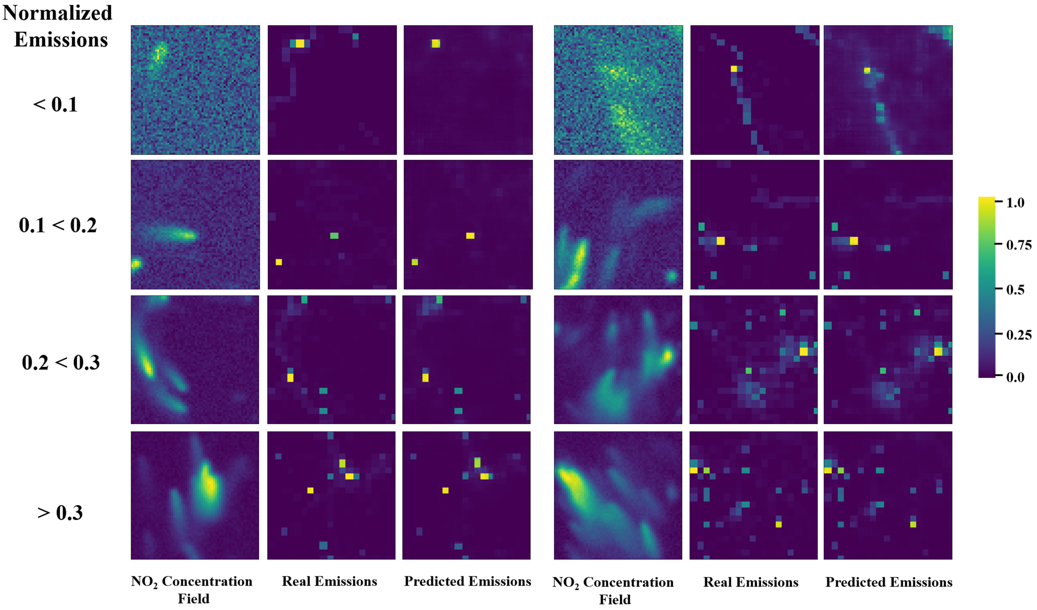
The trained model was applied to the test dataset, which contains more than 36,000 samples. The comparison results are shown in

Table 1. The identification performance of the model on the tested datasets.

Emission Intensity	Detection Accuracy (Top 25%, 1Q)	Detection Accuracy (Top 50%, 2Q)	Detection Accuracy (Top 75%, 3Q)	Count
All	80%	94%	100%	36,938
Low	79%	100%	100%	26,264
Moderate	81%	89%	100%	8222
High	83%	92%	100%	2452

Note: Emission intensity (normalized [0, 1]), All means (0 < emission ≤ 1); Low means (emission < 0.33); Moderate means (0.33 ≤ emission < 0.66); High means (emission ≥ 0.66).

, and the identification results for single and multiple point sources are presented in Figure 5. In Table 1, the emission strength is represented as a relative value, normalized based on the maximum and minimum values across all samples, including the training set, with a range of 0–1. Recognition accuracy refers to the pixel-level accuracy. For example, if the true emission spans 4 × 4 pixels (16 pixels) and the model recognizes an emission of 3 × 4 pixels (12 pixels), the recognition accuracy is 75%. In the table, 1 QR, 2 QR, and 3 QR represent the first, second, and third quartiles, respectively.

As shown in the table, the 1Q correct recognition rate for all emissions was 80%, with more than half of the samples achieving identification rates above 94%. High-emission sources had higher identification accuracy than low-emission sources. For example, the 1Q recognition rate for low emissions (relative emission values below 0.33) was 79%, whereas for high emissions (above 0.66), more than half of the recognition rates reached 83%. The poorer recognition performance for low emissions is primarily due to the indistinct plume shapes, which are more easily obscured by random noise. Overall, the analysis demonstrated that the model achieved good recognition results on the test set, particularly for high-emission point sources.

4.2. Application of TROPOMI Observation Data

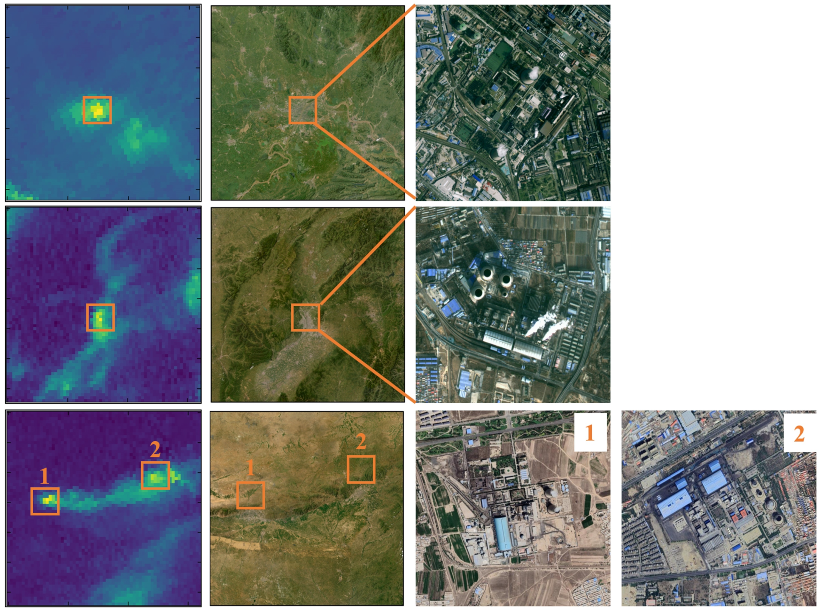
Although the model performs well on the test set, how does it perform on actual observational data? To evaluate this, we used TROPOMI NO₂ data to detect emission source locations. We first tested the model’s performance for large point-source emissions and compared the results with those of the EDGAR data. The outcomes are shown in Figure 6, which displays data from Wuhan on 1 February 2019 (First row), Taiyuan on 4 February (Second row), and Baotou–Hohhot on 5 February (Third row). Overall, the identified emission sources aligned well with the high-value areas in the observed plumes, indicating reasonable results. The results indicate discrepancies between the high emission values in the EDGAR data and the observed plume concentrations. For example, in Wuhan, the EDGAR data indicate two high-emission centers, but the observed NO₂ results show only one. Similarly, in Taiyuan, the EDGAR data suggested a high-emission center in the lower central area, but no corresponding high-concentration region was observed in the TROPOMI data. A similar pattern was observed in the Baotou–Hohhot region. The second column of Figure 6, showing the emission sources identified for the NO₂ plume data, demonstrates that our method effectively identifies high-emission areas, with high-value regions corresponding well to high-concentration areas. We examined the geographical conditions of high-concentration areas and identified high-emission sources such as thermal power plants, as shown in Figure 7.

It should be noted that the model’s ability to detect weak emission areas is limited. This is because small increases in the NO₂ concentration caused by weak emissions can be easily confused with observational errors, resulting in unclear plume shapes.

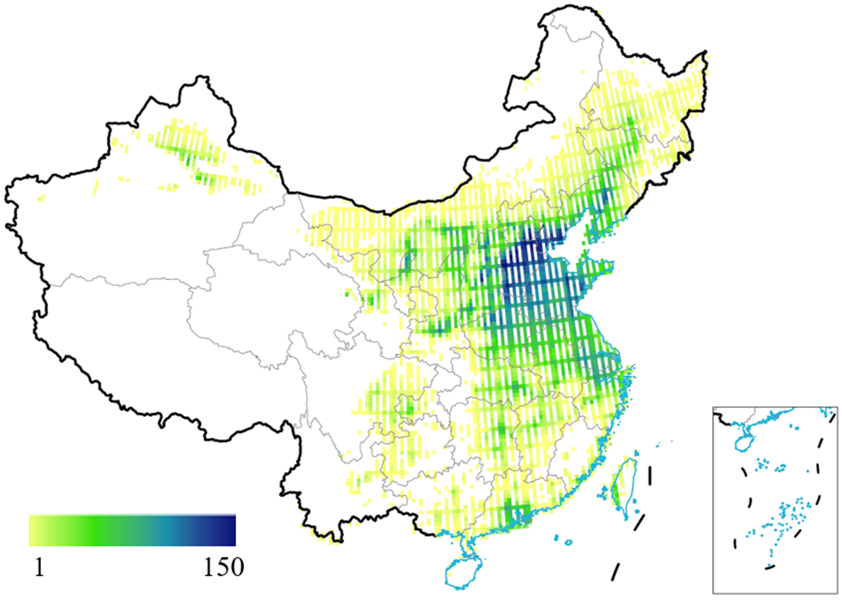
Through analysis, we conclude that the EDGAR inventory lacks timeliness, whereas our model can detect high NO₂ emission sources more accurately and promptly using TROPOMI data. This capability allows for timely updates to the location of emission sources. Furthermore, we extended our application to cover the entire country and compared the detection results in existing inventories, such as MEIC. Figure 8 shows the number of TROPOMI observations for each grid in 2019. A complete observation is defined as covering more than 75% of the grid area. The Beijing–Tianjin–Hebei region has the highest observation frequency, with more than 150 observations annually (over 40% of the days). In contrast, there are fewer observations in the western regions, especially in Sichuan and Tibet, because of the complex terrain, high altitude, and low NO₂ content, making detection more challenging. Figure 9a presents the spatial distribution of NO₂ emissions from MEIC, showing high emission densities in the Yangtze River Delta and the Beijing–Tianjin–Hebei region. In contrast, the NO₂ emissions from Xinjiang, the three northeastern provinces, and Southern China are relatively sparse and scattered. Figure 9b shows the NO₂ emission hotspots detected by the model, excluding detections with relative emission intensities below 0.2 because of poor performance in identifying weak plumes. The results indicate that emission hotspots are concentrated in the Yangtze River Delta and the Beijing–Tianjin–Hebei region, while emissions in Xinjiang, the three northeastern provinces, and Southern China are more scattered, consistent with MEIC observations.

According to statistics, the MEIC emission inventory includes 19 emission hotspots with emissions exceeding 5000 tons/grid (Refer to

Table 2. Identification results of NO₂ hotspot.

Emission (Tons/Grid)	Count of MEIC	Count of Identifications	Identifications Accuracy
>5000	19	17	89%
4000–5000	9	9	100%
2000–4000	82	64	78%
1000–2000	212	143	67%

). Our model successfully identified 17 of these, achieving an accuracy rate of 89%. For hotspots with emissions between 4000–5000 tons/grid, the identification rate was 100%. For hotspots with emissions between 2000–4000 tons/grid, 64 out of 82 were correctly identified, yielding a 78% accuracy rate. However, for hotspots with emissions below 2000 tons/grid, the accuracy dropped further, with 143 out of 212 grids correctly identified, yielding a 67% accuracy rate. Similar to the performance on the test set, the lower accuracy in detecting weaker plumes is mainly due to confusion with observational errors and differences in plume characteristics from the training set. To improve the model’s performance, a more in-depth analysis of the observed NO₂ plume error structures could be conducted, and these insights could be integrated into the simulation data.

Compared to previous qualitative models that only detect the presence or absence of a plume, our proposed model advances quantification by identifying the relative emission intensity. However, this quantification is still preliminary because the conversion of the NO₂ concentration to the emission magnitude is inevitably influenced by simulation errors. To improve the reliability of the simulation results, future work could involve enhancing the simulation mechanism, for instance, by using regional atmospheric transport simulations that account for more factors, leading to more realistic results. Additionally, integrating observational data into the model and assimilating them into the simulation can further improve the accuracy of the concentration-to-emission conversion. Moreover, the weak plume concentrations are easily confused by errors, highlighting the need for further research on weak-plume emission monitoring.

4.3. Correlation Analysis of Industrial NO₂ and CO₂ Emissions

During the high-temperature combustion of fossil fuels, both NO₂ and CO₂ are released simultaneously. Integrating NO₂ data with CO₂ emission estimates can enhance the available observational data and improve estimation accuracy. Currently, remote sensing satellites for point-source CO₂ monitoring, such as Tansat-2 (scheduled for launch in 2025) and CO2M, are still in the development or planning stages, resulting in insufficient observational data for joint satellite remote sensing analysis of CO₂ and NO₂. However, with the successful launch of these satellites, collaborative research on CO₂ and NO₂ emissions is expected to become an emerging research focus.

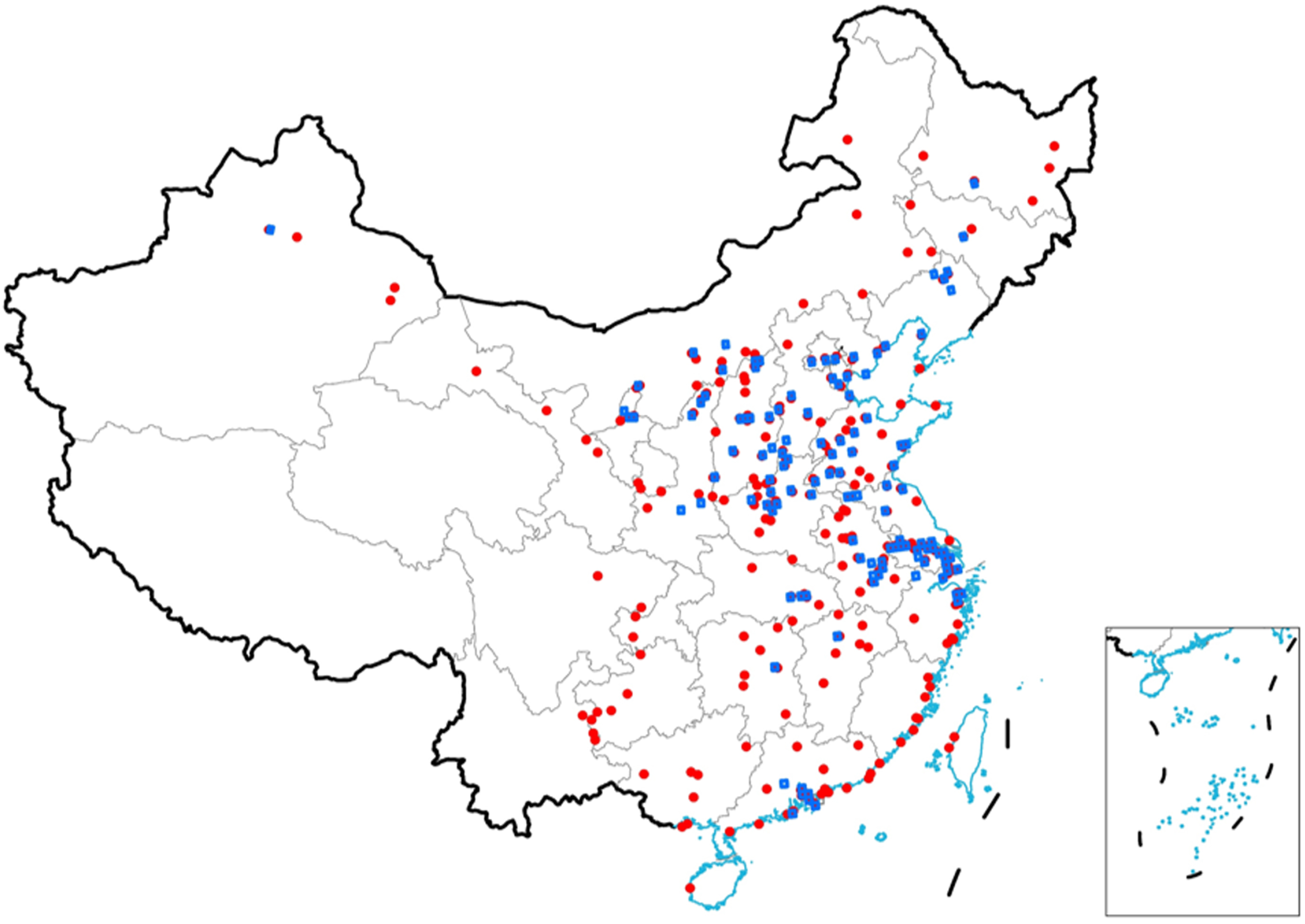
The detected NO₂ emission hotspot areas overlap with the CO₂ hotspot areas to some extent. To analyze this, we combined the data with ODIAC to assess their correlation. ODIAC includes emission sources such as thermal power plants and households, with a spatial resolution of 1 km × 1 km. First, we identified and plotted further CO₂ emission points in the ODIAC, with a monthly emission of approximately 100,000 tons/grid/month, as shown in Figure 10. The red dots in the figure represent high-emission sources in the ODIAC, while the blue boxes highlight areas where NO₂ hotspots overlap with CO₂ hotspots. Overall, there are about 252 high-emission CO₂ sources in the ODIAC and 102 areas where NO₂ and CO₂ hotspots overlap, accounting for approximately 40% of the total. In the East China region, the overlap between NO₂ and CO₂ hotspots is more prominent, accounting for over 60% of the cases, whereas the identification performance is weaker in the southwest region. Combining Figure 8, the main reasons for the missed detections are: (1) This is related to the effective coverage of the original data. There were fewer observations in the southwest region, whereas the observation frequency was higher in East China and Guangdong. As a result, more NO₂ plumes and CO₂ hotspots that meet stringent screening conditions were detected in East China and Guangdong, whereas fewer were detected in the southwest region. (2) The detection algorithm may not be sufficiently accurate for weak plumes, potentially leading to the omission of weak emissions and, consequently, the neglect of some emission hotspots.

Overall, our detection method performed well at identifying NO₂ emission hotspots under high-emission and high-frequency observation conditions, with a good degree of overlap with CO₂ emission hotspots. However, in low-frequency observation and weak emission scenarios, the algorithm’s sensitivity is insufficient, highlighting the need for further improvements to enhance its ability to detect weak plumes.

4.4. Limitations

Deep learning methods have great potential for the global carbon stocktake. In this study, we propose a deep-learning-based approach for identifying industrial CO₂ emission point sources, achieving the preliminary identification of emission locations and their relative magnitudes. However, due to the current limited understanding of instrument errors, inversion errors, and atmospheric transport simulation errors, it is challenging to accurately account for their impact when estimating absolute emissions. In future work, we will conduct an in-depth study of various error characteristics and propagation patterns, quantify their impact on emission estimates, and provide uncertainty ranges alongside emission estimates. In the future, we plan to apply this model to a longer time series of TROPOMI data to assess improvements in China‘s emission reduction policies by analyzing changes in detected emission hotspots.

5. Conclusions

To overcome the current limitations in available observational data for global CO₂ emission hotspot monitoring, and leveraging the co-emission of NO₂ and CO₂ from industrial sources, we propose a method for detecting NO₂ hotspots using convolutional neural networks (CNNs). This approach provides valuable prior information for detecting CO₂ emission hotspots. The key contributions of this study are as follows: (1) We utilized atmospheric dispersion models to generate a wide range of simulation scenarios, creating training data for NO₂ plume detection and addressing the issue of missing samples in existing NO₂ hotspot detection. (2) We developed a suitable network architecture based on a convolutional neural network model for hotspot detection and applied it to satellite-observed data. (3) We analyzed the correlation between NO₂ emission hotspots and CO₂ hotspots. The results demonstrate that our algorithm effectively identifies emission hotspots in high NO₂ emission areas under multiple observation conditions, achieving an overlap rate of over 80% with existing NO₂ emission inventories. In East China, where observations are more frequent, significant overlap is observed between NO₂ and CO₂ emission hotspots, with NO₂ hotspots acting as indicators for CO₂ emission regions. However, the study also reveals some limitations, particularly in the detection sensitivity for weak NO₂ emission sources, where the performance of the detection algorithm is constrained. This represents an area for further improvement in future work.

When using Tansat-2 and CO2M for point-source and urban CO₂ remote sensing monitoring, a large volume of collaborative CO₂ and NO₂ observation data will be generated. The monitoring methods developed using deep learning models provide fast and reliable reference information for preliminary data analysis and screening, enabling efficient management of the anticipated data growth. Additionally, this approach offers a technical solution for transitioning from “concentration-to-emission” estimates based on atmospheric transport models to those derived from deep learning models.