Article

Harnessing InSAR and Machine Learning for Geotectonic Unit-Specific Landslide Susceptibility Mapping: The Case of Western Greece

by
Stavroula Alatza
1,2,*,
Alexis Apostolakis
2,3,
Constantinos Loupasakis
1,
Charalampos Kontoes
2,
Martha Kokkalidou
2,
Nikolaos S. Bartsotas
2 and
Georgios Christopoulos
2
1
Laboratory of Engineering Geology and Hydrogeology, School of Mining and Metallurgical Engineering, National Technical University of Athens, Zografou, 157 80 Athens, Greece
2
National Observatory of Athens, Operational Unit BEYOND Centre for Earth Observation Research and Satellite Remote Sensing IAASARS/NOA, 152 36 Athens, Greece
3
School of Electrical and Computer Engineering, National Technical University of Athens, Zografou, 157 80 Athens, Greece
*
Author to whom correspondence should be addressed.
Remote Sens. 2025, 17(7), 1161; https://doi.org/10.3390/rs17071161
Submission received: 24 January 2025 / Revised: 19 March 2025 / Accepted: 21 March 2025 / Published: 25 March 2025
(This article belongs to the Special Issue Remote Sensing in Natural Hazard Exploration and Impact Assessment)

Abstract

:
Landslides are one of the most severe geohazards globally, causing extreme financial and social losses. While InSAR time-series analyses provide valuable insights into landslide detection, mapping, and monitoring, AI is also implemented in a variety of geohazards, including landslides. In the present study, a machine learning (ML) landslide susceptibility map is proposed that integrates the geotectonic units of Greece and incorporates various sources of landslide data. Satellite data from Persistent Scatterer Interferometry analysis, validated by geotechnical experts, resulted in an extremely large dataset of more than 3000 landslides in an area of interest, including the most landslide-prone area in Greece. The gradient-boosted decision tree was employed in the landslide susceptibility mapping. The model was trained on three geotectonic units and five prefectures of Western Greece and performed well in predicting landslide events. Finally, a SHAP (SHapley Additive exPlanations) analysis verified that precipitation and geology, which are the main landslide-triggering and preparatory factors, respectively, in Greece, positively affected landslide characterization. The innovation of the proposed research lies in the uniqueness of this newly created dataset, comprising a remarkably large number of landslide and non-landslide locations in Western Greece. By adopting a strict machine learning methodology, the spatial autocorrelation effect, which is overlooked in similar studies, was reduced. Also, leveraging the unique features of the geological formations, the model was trained to incorporate differences in the landslide susceptibility of formations located in different geotectonic units with variant geotechnical characteristics. The proposed approach facilitates the generalization of the model and sets a strong base for the creation of a national-scale landslide susceptibility mapping and forecasting system.

Graphical Abstract

1. Introduction

Landslides (LS) are considered among the most destructive natural hazards worldwide. Extreme precipitation events due to climate change, urbanization and urban activities, deforestation, and seismic activity are some of the most common triggering factors of landslides [1,2]. Greece, specifically due to its intense geomorphology and as one of the most active geotectonically regions in Europe, is among the most landslide-susceptible regions in the Mediterranean. SAR interferometry is widely applied in a variety of surface deformation monitoring [3,4,5], including landslide detection and monitoring [6,7,8]. InSAR stacking techniques [9], used to identify activities of landslides, as well as polarimetry and coherence [10], coherence change detection [11], Persistent Scatterer Interferometry [12,13,14,15], and Small Baseline Subset [16], are some of the most widely applied SAR techniques for landslide mapping and monitoring. On the other hand, AI has rapidly proved its efficiency in accurately predicting landslide-prone units or providing a landslide early warning system [17]. Many AI algorithms, with the majority of them being tree-based ensemble models, have been employed in the field of landslide susceptibility mapping. Specifically, machine learning models provide significant advantages in terms of accuracy, scalability, and adaptability compared to traditional landslide susceptibility methods. ML can efficiently detect nonlinear relationships between causal factors and identify the most important ones. They can also handle big volumes of data and adapt to different areas through fine-tuning. Support vector machines (SVM) [18,19], Random Forest (RF) models [20,21], and extreme gradient boosting (XGBoost) models [22,23,24] are among the most commonly used ML models for landslide detection and susceptibility mapping. A comparison of the efficiency between different ML models is commonly performed in landslide susceptibility studies using ML models [25,26,27]. Also, Ferreira et al. [28] performed a comparison between multi-criteria analysis (MCA) and ML for landslide susceptibility mapping. Deep learning models have also proved to be efficient in landslide susceptibility studies [29,30]. A common pitfall in many related studies (e.g., [22,31,32,33,34]) is the oversight of spatial autocorrelation [35]. Typically, datasets are split into training, validation, and test sets, but these sets often overlap spatially. This results in nearby, similar data points appearing in both the training and validation/test sets, leading to high-variance models with poor generalization ability, as explained in [35,36].
Over the past decade, ML has been widely applied in landslide susceptibility mapping and prediction. Key challenges include model migration to new areas or larger scales and the limited size of training and validation datasets, which can significantly impact model performance. The uniqueness of the proposed research lies, on the one hand, in the exceptionally large landslide inventory created, covering a broad area in Western Greece. This includes more than 3000 landslides validated by applying ground truth or remote sensing techniques. The innovation of the proposed research lies in the uniqueness of this newly created dataset, which comprises a remarkably large number of landslide and non-landslide locations in Western Greece, covering five prefectures. Adapting the model to the unique characteristics of Greece’s geotectonic units and scaling it nationally shows great promise for improving the generalization and accuracy of landslide susceptibility predictions, as demonstrated by this research. The division of Greece into geotectonic units and the addition of the geotectonic unit as an influencing factor is another innovative aspect that has never been tested before.
We demonstrate the informativeness of this dataset by training an XGBoost model to predict landslide susceptibility and applying a strict machine learning methodology. To improve the model’s generalization ability, along with n-fold cross-validation and hyperparameter tuning, we applied a buffer filtering technique to reduce spatial autocorrelation, minimizing its impact on training and performance. As a further step, the SHAP (SHapley Additive exPlanations) methodology was applied to validate that the model’s decisions were aligned with domain-specific knowledge.
Finally, the exploitation of PSI enriched the landslide inventory, serving as a validation tool for the model’s predictions, highlighting the remarkable potential of combining remote sensing techniques and data with AI.

2. Materials and Methods
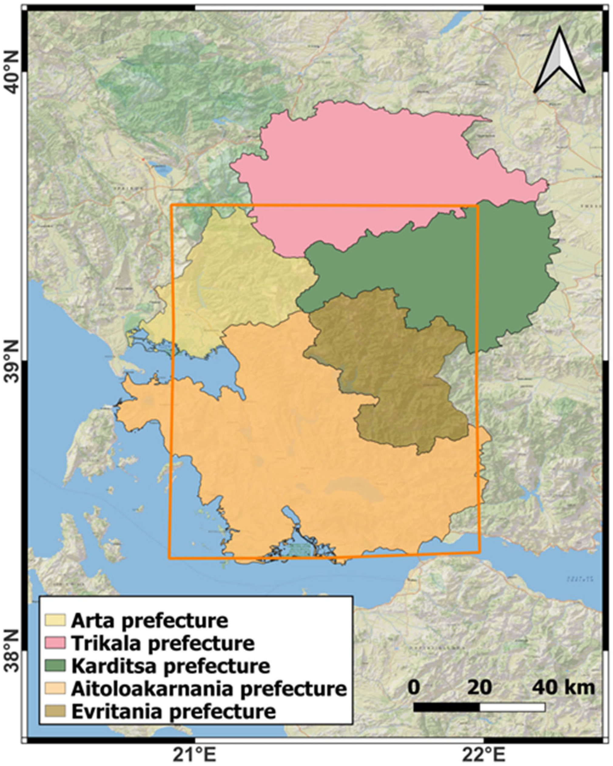
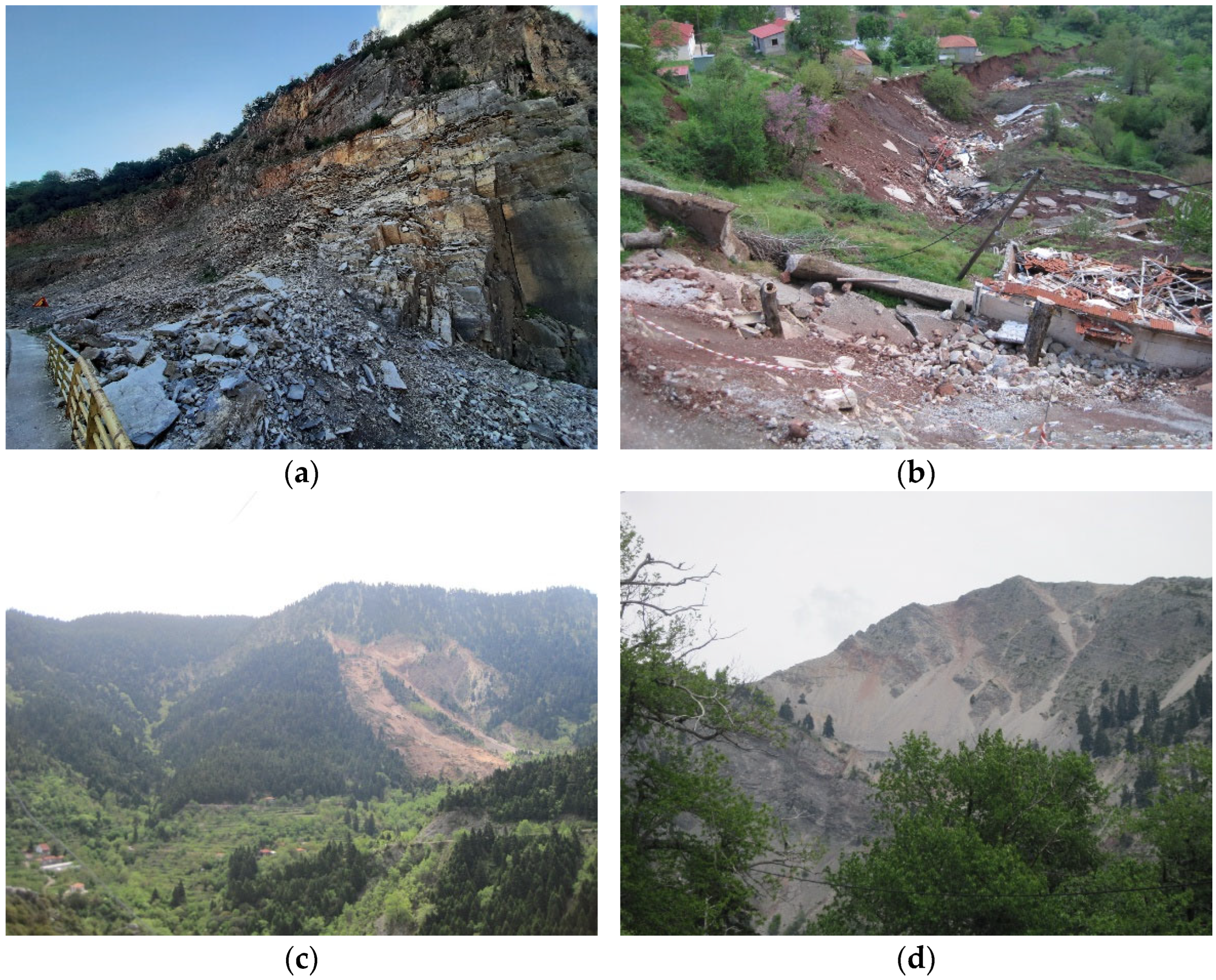
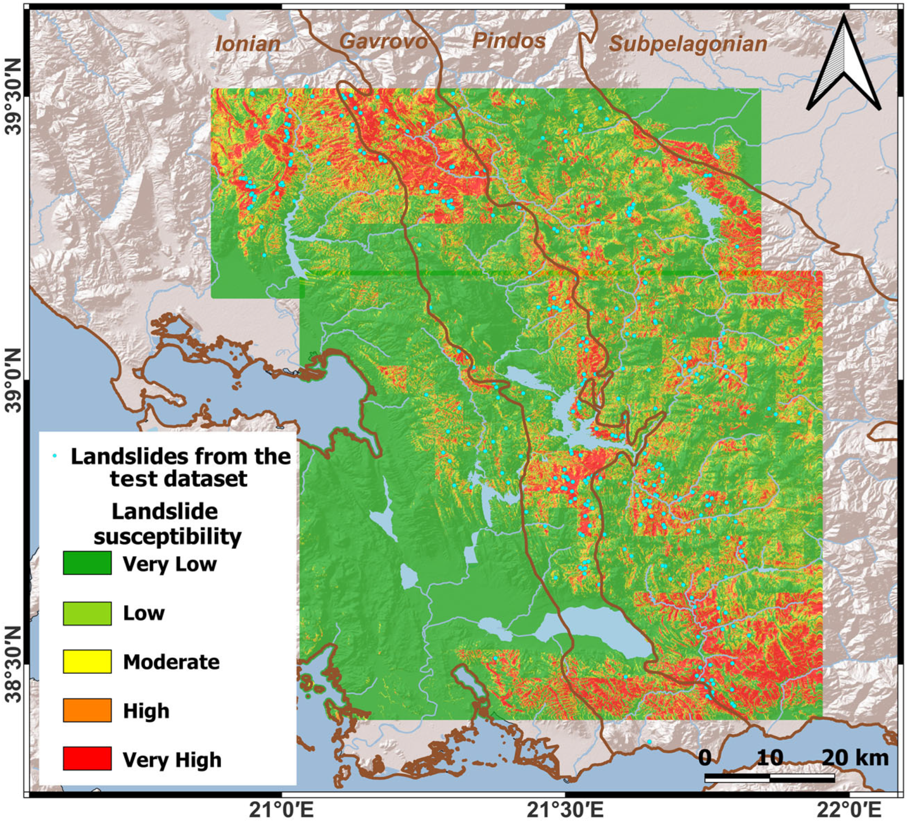
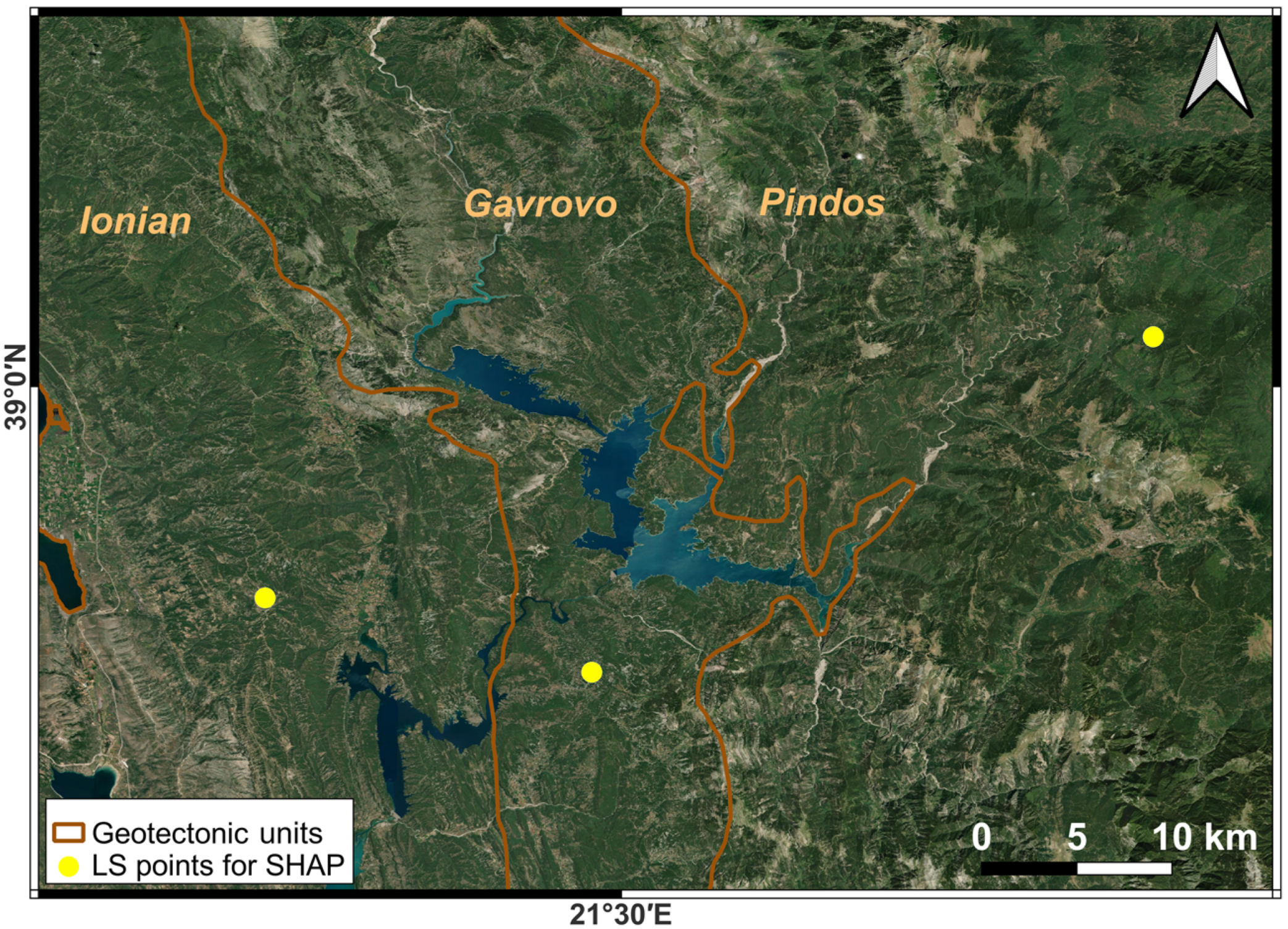
2.1. The Study Area

The study area is located in Western and Central Greece, encompassing a significant portion of the Pindus mountain range. It covers an area of 12,000 km2 and includes five prefectures, namely Aitoloakarnania, Evritania, Trikala, Arta, and Karditsa (Figure 1), as well as three geotectonic units, Pindos, Gavrovo, and Ionian (Figure 2). This particular location was chosen due to its notable variations in landslide occurrences. The Pindos geotectonic unit stands out as the most landslide-prone region in Greece, accounting for over 40% of the total recorded cases [1]. In contrast, Gavrovo and Ionian exhibit significantly lower frequencies of landslides, with occurrences of 4% and 4.5%, respectively [1,37]. From a geotectonic point of view, the Pindos, Gavrovo, and Ionian units are part of the External Hellenides, which cover the Central and Western regions of Greece. The External Hellenides are occupied by formations younger than those of the Internal Hellenides [38]. These geotectonic units are predominantly composed of Mesozoic and Cenozoic deep-sea and shallow-water sedimentary rocks, limestones, and dolomites without any important metamorphism [38]. This carbonate sedimentary process was terminated with a Paleocene to Miocene flysch deposition [38,39]. These deposits exhibit the presence of strong E-W compressional tectonic movements, resulting in the Pindos unit thrusting over the neighboring unit of Gavrovo, as well as intense folding and fracturing [39,40,41]. The westward-directed over-thrusting associated with the Alpine orogeny was followed by a prevailing N-S extensional ground deformation [42], which formed extensive trances that, during the Paleogene and the Neogene, were filed by Molasse and Marl formations, respectively [39,43,44]. Also, Quaternary deposits can be identified along the plain areas of the study area and the coastal zone of the Corinthian Gulf [38].
Rock slope instabilities are prevalent in flysch formations, primarily attributed to factors such as heterogeneity, the presence of silty-clayey members with low strength, significant tectonic disturbance, and the weathering degree [45]. At the Pindos geotectonic unit, the combination of intense tectonism [46], steep slopes, the highly susceptible flysch, and high precipitation levels contribute to an enhanced occurrence of slope failures. Conversely, in the Gavrovo and Ionian geotectonic units, the presence of less intense tectonism, occurring in the sequence of mega-synclines and mega-anticlines [40], and the prevalence of limestone formations decreases the frequency of landsliding.

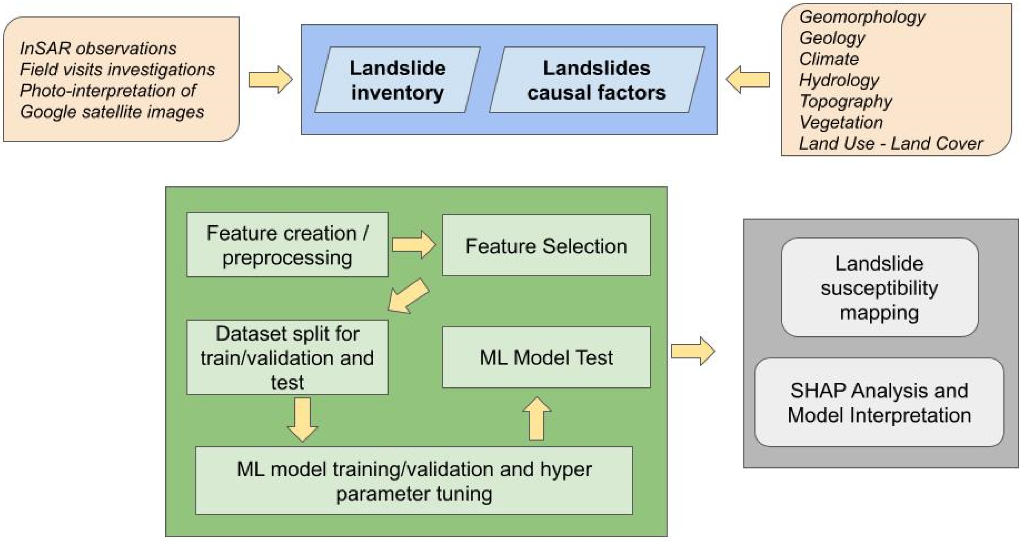
2.2. Landslide Inventory

Several sources of landslides (Table 1 and Figure 3) were introduced in the current ML landslide susceptibility model. First, landslide locations from [6] were used in the present study. Specifically, in Kontoes et al. [6], 245 landslides were identified by the LOS displacements acquired by the processing of ERS and ENVISAT sensors, covering the periods from 1992 to 2000 and 2003 to 2010, respectively. Also, in Kontoes et al. [6], 397 landslide locations were provided by the Hellenic Survey of Geology and Mineral Exploration (HSGME). The 397 landslides from the HSGME were enriched by 704 more landslides that were identified by visual inspection of satellite images by a geotechnical expert. A total of 2354 landslides were detected by the LOS displacements from the InSAR Greece product [47]. InSAR Greece is a nationwide project for mapping LOS displacements in Greece with the use of Sentinel-1 images. LOS displacements were mapped by processing Sentinel-1 SLCs from 2015 to 2019 with a parallelized version of the Stanford method for Persistent Scatterers Interferometry [48], the so-called P-PSI [47]. The P-PSI is a fully automated InSAR processing chain that is developed and operates at the Operational Unit BEYOND Centre for Earth Observation Research and Satellite Remote Sensing of the National Observatory of Athens.
For distinguishing possible landslide locations from the PS points, initially PSs with negative LOS displacements lower than −2 mm/y were selected. At a later stage, those scatterers were validated by a geotechnical expert. The selected PSs were validated by photointerpretation using open-access sources (e.g., street view images) and Google satellite images. Additional validations were provided by field visit inspections of the Evritania and Aitoloakarnania prefectures (Figure 4). Permanent scatterers, identified as potential landslide locations within a buffer zone smaller than 20 m, were combined into a single point, representing one consolidated landslide location. Overall, a total of 3700 landslides were identified for the area of interest, which is an exceptional number for a landslide inventory. For the selection of non-landslide locations, the same rationale for identifying the LS locations from the Greece InSAR product was followed. PS points with almost zero deformation were identified and also validated by an expert.
Buffers of several sizes, ranging from 200 m to 1 km, were tested around the LS locations for selecting no LS locations. In our study area, a buffer of 600 m proved to be effective in avoiding the wrong labeling of the PS points. In the selection of non-landslide points, two aspects were taken into consideration. First, the number of landslide (LS) and non-landslide (non-LS) points was adjusted to achieve a balanced distribution, ensuring equal representation in the dataset. Second, the distribution of LS and non-LS points was chosen to be as homogeneous as possible, considering the special geophysical characteristics of the study area.
Furthermore, a buffer of 300 m around every LS and no LS point was applied to limit data leakage due to spatial autocorrelation. Spatial autocorrelation occurs when two points in close proximity with similar feature values are included in both the training and validation (or test) sets [35]. Furthermore, the application of the buffer resulted in a downsampling of the dataset. Specifically, the LS locations were affected, and it led to an LS-non-LS ratio of 1:3. Therefore, from the initial 3700 LS locations, after excluding LS points from the applied buffers and dropping all the duplicates, the final landslide dataset consisted of 1375 landslides (Figure 5). Similarly, 3833 non-landslide locations were introduced in the landslide susceptibility ML model (Figure 5).

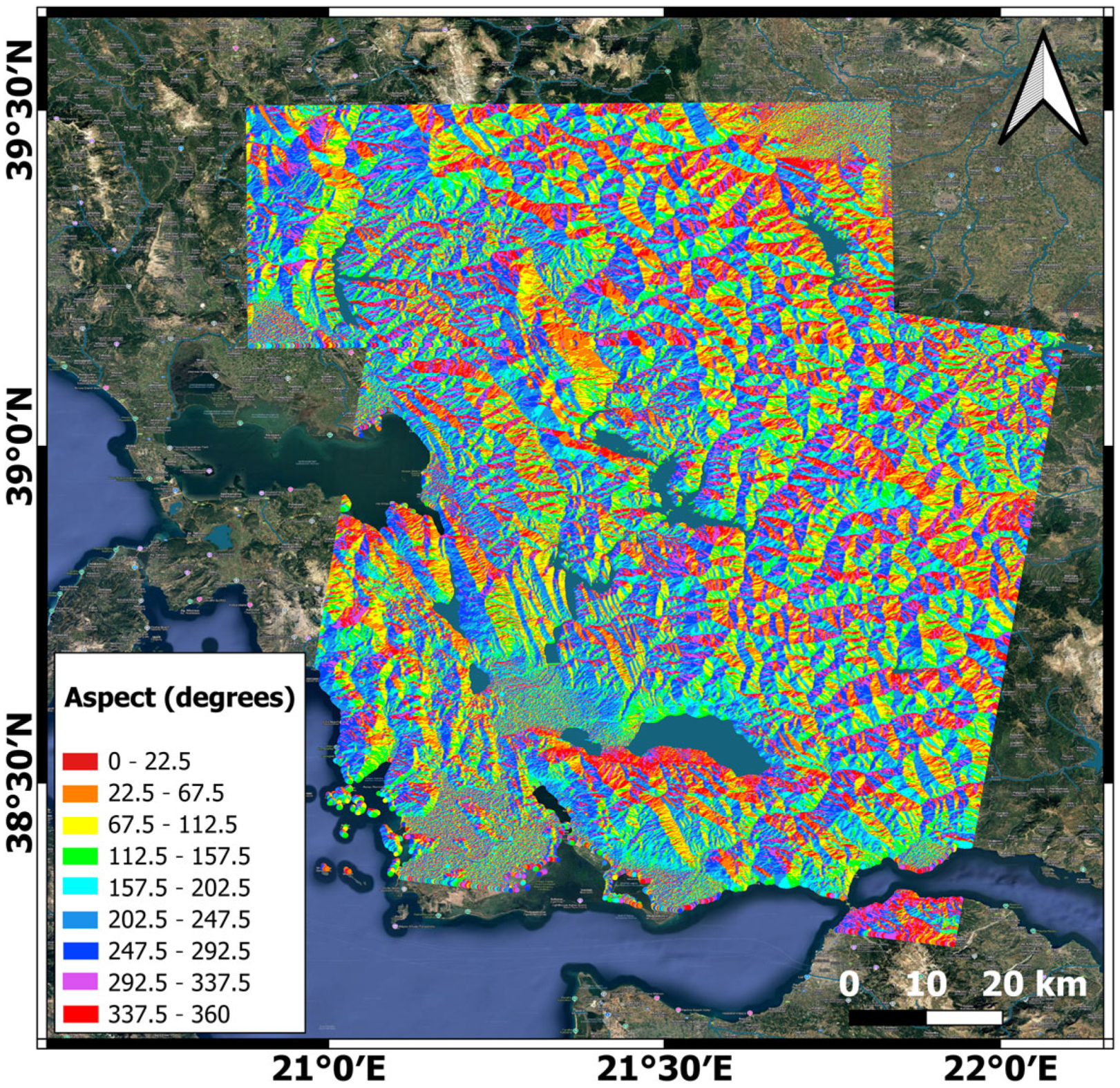
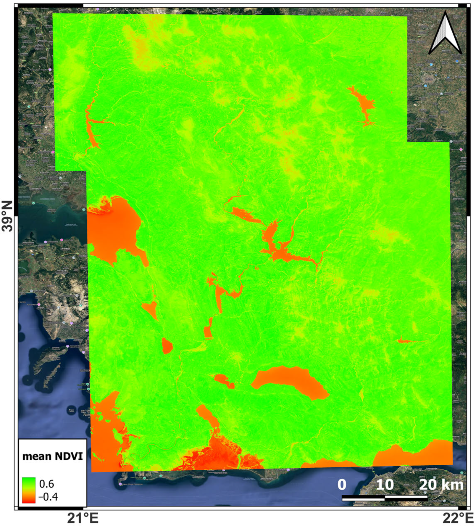
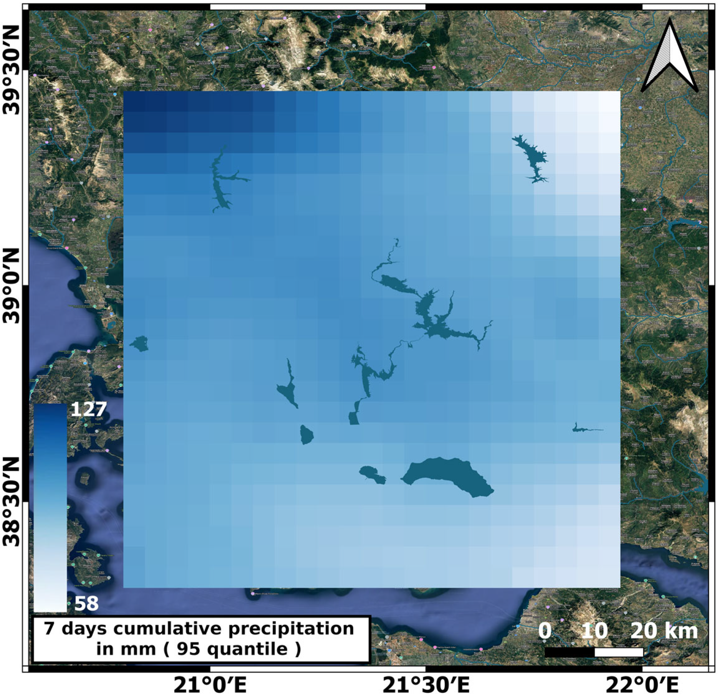
2.3. Landslide Causal Factors

Landslide causal factors are both natural and anthropogenic. According to an extended literature review, the most common landslide causal factors are divided into topography, geomorphological, hydrological, and climate factors. It is also important to mention that these factors may differ from one area to another and between different types of landslides. Therefore, to determine which causal factors have a serious impact on a landslide risk assessment, an extensive analysis is required. Geology [49], earthquakes [50], and rainfall [51,52] are some of the most common landslide causal factors (preparatory and triggering) in Greece. It is worth noting that the study area experiences high precipitation rates. Based on [53], higher precipitation levels are recorded in areas west of the Pindus and in Western Greece, while lower precipitation levels are observed in Central and Eastern Greece. In the present study, the landslide causal factors that were introduced to the model are summarized in Table 2.
Referring briefly to the examined causal factors, topography has a direct effect on ground failures and instabilities. Aspect, slope, elevation, and terrain roughness were selected as topography factors. Slope represents the level of inclination of a surface with respect to a flat surface, measured in degrees. Aspect represents the direction of a surface, also measured in degrees. Aspect does not have a direct effect on landslides; however, the direction of a slope has an impact on the micro-climate, vegetation, and land cover, in general, due to exposure to different climate conditions [54,55]. Elevation (altitude) is another important causal factor of landslides, as mountainous areas at high altitudes are affected more intensively by high and prolonged precipitation rates. Terrain roughness, land use–land cover, surface lithology, and the slope length (LS) factor are also selected among the causal factors that affect landslides. A further analysis of the above-mentioned causal factors is provided below.
Regarding the impact of the LS factor on landslide susceptibility, according to the RUSLE model developed by Wischmeier and Smith (1978) [56], the S-factor corresponds to the slope steepness and the L-factor to the slope length. Both factors are associated with soil erosion; therefore, they can also be associated with landslide susceptibility. The impact of lithology, as one of the most important parameters in landslide occurrence, is widely investigated [57]. In the investigated area, there is a wide variety of geological formations and morphological features.
Finally, land cover provides valuable insights into the type of elements, natural or manmade, in the investigated area. Therefore, changes in land cover seriously affect landslide susceptibility.
The absence of vegetation cover can be considered an indicator of a landslide-susceptible area. Peduzzi et al. [58] concluded that the NDVI is an important parameter for introducing into a landslide susceptibility model.
The Topographic Wetness Index, Terrain Roughness Index, Stream Power Index, and Sediment Transport Index were also introduced into the model as causal factors. The Topographic Wetness Index, calculated from the DEM, is used as an indicator of soil moisture. The Terrain Roughness Index indicates the surface roughness. The Stream Power Index is associated with the erosive power of water flow. The Sediment Transport Index is a measure of the flow capacity to transport sediments.
All parameters are estimated and introduced in the LS susceptibility model, derived from open-source data, to facilitate the projection of the current research at a larger scale project. The EU-DEM [59] was employed for the estimation of the geomorphological factors, with a resolution of 25 m. In all parameters computed as raster layers, a 25 m pixel size was used in order to maintain the same resolution for all layers. Slope length information about the area of interest was used and retrieved from the EUROPEAN SOIL DATA CENTRE (ESDAC) [60]. Land use and land cover data were used and retrieved from Copernicus Corine Land Cover 2018 [61]. For the land use–land cover, the second level of classification of Corine Land Cover product was employed. The land cover parameter was reclassified (Table A4). Surface lithology was employed by the EGDI 1:1 Million pan-European Surface Geology INSPIRE Conformant National WFS services on the GeologicUnit [62]. Snow melt was used and retrieved from ERA5–LAND [63], with a spatial sampling of 9 km. The topographic and hydrological parameters were estimated using the Slope product derived from the EU-DEM. Finally, a mean value of the Normalized Difference Vegetation Index (NDVI) from 2000 to 2020, computed in the Google Earth Engine using MODIS data [64], was also introduced as a landslide causative factor. A Climate Hazards Group InfraRed Precipitation with Station data (CHIRPS) validated precipitation product, that blends satellite observations with in-situ measurements from rain-gauges, was used as precipitation data covering a time period from 2000 to 2020. The spatial sampling of the precipitation data is 5 km.

2.4. Machine Learning Pipeline

The methodology followed to establish a ML model with a high generalization ability to unseen areas is presented in Figure 6 and analytically described in the following sub-sections.

2.4.1. Problem Formulation and Algorithm

It is important to evaluate the prototype dataset’s potential for exploitation by machine learning algorithms. The instances of the dataset are uniquely determined by each point coordinate and are labeled with a binary class as follows: positive (“Landslide”), denoting the existence of a landslide, or negative (“No landslide”), denoting the absence. Points are also assigned with a vector containing the values of the triggering factors at the specific location. Hence, the problem is formulated as a binary classification, as the model will learn to grade its decision in favor of one of the classes according to the feature vector. XGBoost is selected to train a baseline model because it is one of the most popular algorithms in the category of ensemble learning, and it leverages the boosting technique, which has important advantages over bagging (e.g., Random Forest). It is designed for sequential training, creating, in each step, new weak learners that focus on less successful predictions, thus reducing the error in each step of the algorithm. This technique leverages the discovery of more complex relationships among features, thus reducing bias more effectively than the bagging techniques. Furthermore, XGBoost has an advantage over previous representatives of boosting like AdaBoost and Gradient Boosting by incorporating regularization techniques (Lasso-1 and Lasso-2) that prevent overfitting.

2.4.2. Feature Selection and Preprocessing

Feature selection is an important part of the landslide classification problem, as the selection of the parameters that mostly affect the occurrence of landslides can seriously affect the model’s performance and predictions. Factors with no correlation can be a source of noise that may seriously affect the model’s performance and the landslide susceptibility map. Ranking methods were applied in order to have an overview of the possible associations between the selected factors and to exclude uncorrelated features from model training. The Pearson correlation coefficient was used to analyze the correlation of the dataset’s features. The Pearson correlation matrix of the selected features is presented in Figure S1 (Supplemental Materials). The selection of the final contributing factors was finalized after several model trainings and feature importance calculation. Regarding the various scales of the input features, an additional preprocessing step was normalization, using a standard range from −1 to +1. One-hot encoding was also applied since the influencing factors include both numerical and categorical data, as presented in Table 2.

2.4.3. Dataset Split for Training, Validation and Testing, and Hyperparameterization

As described in Section 2.2, a 300 m buffer was applied to mitigate spatial autocorrelation, which, if unaddressed, can degrade a model’s generalization to unseen areas. However, it is worth noting that several studies [22,31,32,33,34] overlook this issue by randomly shuffling the initial dataset to create test and validation sets, inadvertently causing information leakage due to similar instances appearing in both sets [35]. From the 5208 landslides and no landslide locations, 80% were used for the training dataset (3191 points), whereas 20% (1219 points) were used for the unseen test dataset. The training dataset was split again for cross-validation five-fold, and then cross-validation with hyperparameter tuning using Grid Search was applied. The dataset split ratio is presented in Figure 7a. The XGBoost parameters that provided the best results during cross-validation were as follows: column sampling (colsample_bytree) = 0.8, γ (gamma) = 0.7, learning_rate (learning_rate) = 0.1, max_tree_depth (max_depth) = 9, minimum sum of instance weight (min_child_weight) = 5, number of trees (n_estimators) = 270, L1 regularization (reg_alpha) = 0, L2 regularization (reg_lambda) = 1, imbalanced factor (scale_pos_weight) = 1, and proportion of training data (subsample) = 1. We note that the L1 regularization parameter was set to 0, indicating that the XGBoost model does not find it beneficial to penalize specific features. This suggests that the features are well-chosen and contribute meaningfully to the model’s predictions. Furthermore, to highlight the importance of addressing spatial autocorrelation, a second dataset split setting was used, where the test was in a remote area, spatially separated from the training/validation dataset area (Figure 7b).

2.4.4. Train/Validation Test Datasets Visualization
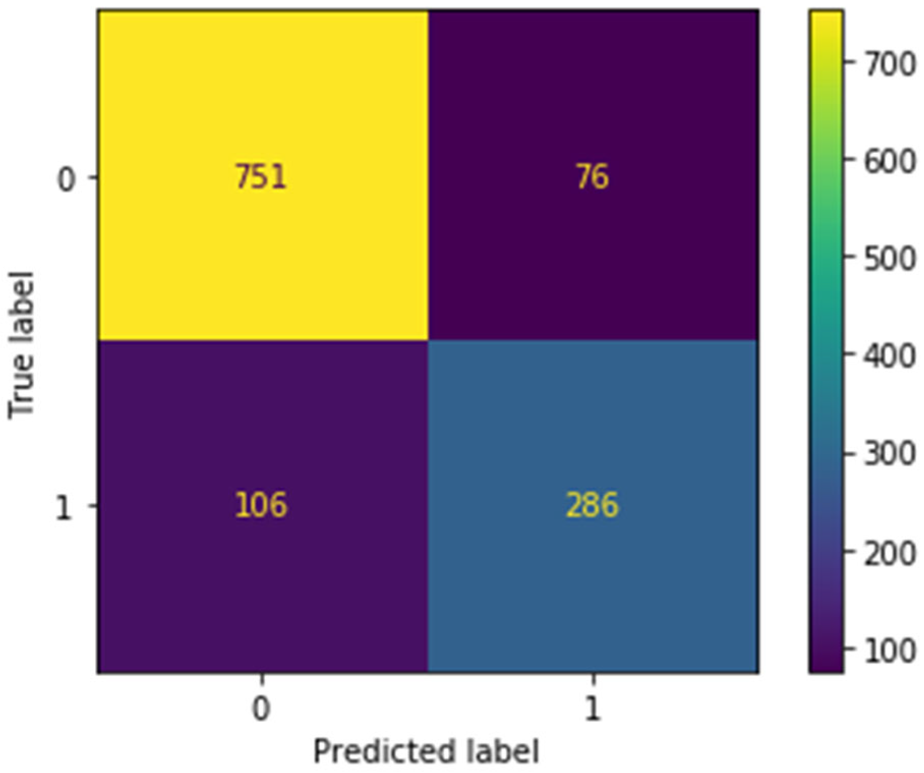
From Figure 5, it is apparent that the majority of the landslides (2991) are located in the Evritania and Aitoloakarnania prefectures. Following the rationale of geotectonic unit indexing of the landslide dataset, 200 more landslides located in the Arta, Trikala, and Karditsa prefectures (Figure 1) and within the boundaries of the Ionian, Gavrovo, Pindos, Subpelagonian geotectonic units, were added to the main landslides inventory in the Evritania and Aitoloakarnania prefectures.
Figure 7a represents the main train/validation test split setting. It is apparent that the training/validation dataset area overlaps with the test dataset area. In Figure 7b, the split setting is designed to showcase the effect of spatial autocorrelation on the model results. Here, the test dataset is located in a remote area, with practically no spatial correlation between the two sets. This figure shows the dataset created after the application of the 300 m buffer (training/val. no LS: 3006, training/val. LS: 983, test no LS: 827, test LS: 392). The unbuffered dataset has the same pattern that is seen in this figure but has more dense points (training/val. no LS: 34,442, training/val. LS: 3224, test no LS: 262, test LS: 208).

3. Results

Model evaluation is vital in machine learning to ensure reliable predictions, but its importance is amplified in geohazard applications. Here, model performance directly influences critical decision-making in risk management. Rigorous evaluations ensure the model excels not only on the training data but also on unseen scenarios, safeguarding its practical reliability and impact.

3.1. Results for Main Split Setting

The XGBoost model, used for landslide predictions, was mainly evaluated based on precision, recall, F1, and Mathew’s correlation coefficient (MCC) metrics. The model’s evaluation metrics are provided in Table 3. MCC takes into account all four components of the confusion matrix (true positives, true negatives, false positives, and false negatives) [65]. Unlike accuracy, it is not misleading when dealing with imbalanced datasets. MCC score ranges from −1 to 1, where −1 indicates a completely incorrect classification, 0 represents random performance, and 1 signifies perfect classification. For example, a MCC value of 0.65 suggests that both recall (sensitivity) and specificity are fairly high, meaning that the model is correctly identifying a significant proportion of both positive and negative classes. It is worth noting that the performance on the unfiltered 300 m dataset (see Section 2.2 and Section 2.4) was higher, with a recall of 0.95 and a precision of 0.85. However, as explained in Section 2.2 and Section 2.4, data leakage due to spatial correlation would result in a model with poor generalization, which contradicts our goal. Therefore, we present the results of the more robust model, trained on the filtered dataset, that better generalizes to unseen areas.
Based on the precision results of the model, 79% of the predictions were true positive. Based on the recall of the model, 73% of the identified landslides were actual events. Also, the high F1 score verifies the ability of the model to effectively identify actual landslide events and minimize false positive events. Higher scores are observed in the no landslide predictions (Table 3).
A confusion matrix was also used to assess the model’s performance (Figure 8). A confusion matrix consists of four components, which are the following: true positives (TP), true negatives (TN), false positives (FP), and false negatives (FN). Figure 8 indicates that the model performed well in identifying TN events, which are actual non-landslides, and TP events that correspond to actual landslide events in both the test and validation datasets. Also, the numbers of correctly predicted landslide and no landslide positions are almost equal, indicating that the model learned equally well to distinguish between landslide and no landslide events.
The landslide susceptibility map, based on predictions on a grid with a cell size of 25 m, is presented in Figure 9. The landslide locations of the validation dataset are also added as an indicator of the model’s performance. From Figure 9, it is apparent that the majority of landslides are presented in the Pindos and Gavrovo units, where landslide occurrences are more frequent. Also, accurate predictions were performed in the Subpelagonian unit, where only a few locations were used as a training test, and the majority of landslides were added to the validation dataset. Five susceptibility levels have been produced from a five-range binning of the model’s score (0.0–0.2, 0.2–0.3, 0.3–0.4, 0.4–0.7, and 0.7–1). The model is configured to produce an output in the continuous range [0–1] that reflects the model’s confidence in the likelihood of a landslide class (1). However, it is important to note that this score should not be directly interpreted as the probability of a landslide.

3.2. Results for Test Split in Remote Area
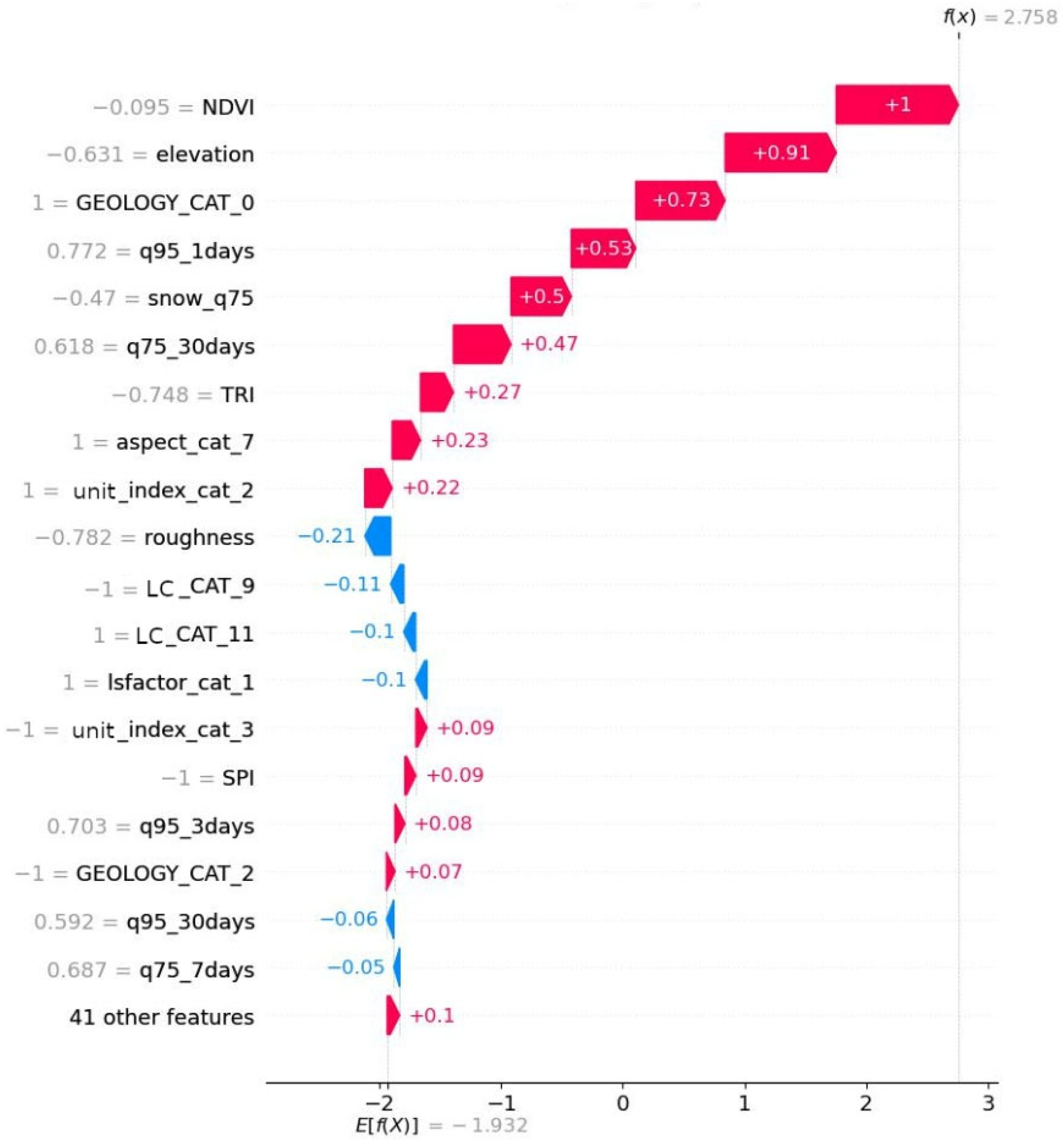
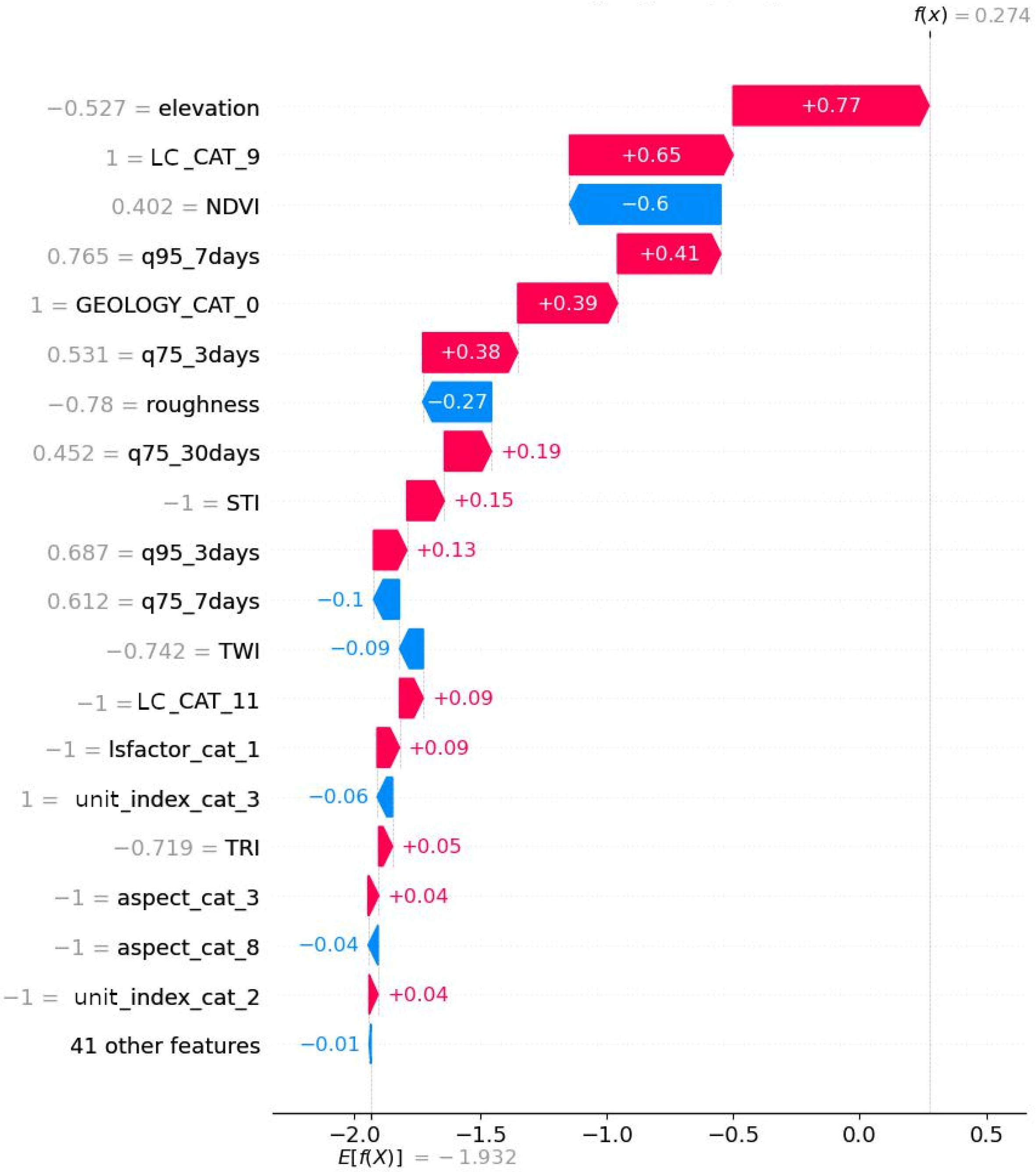
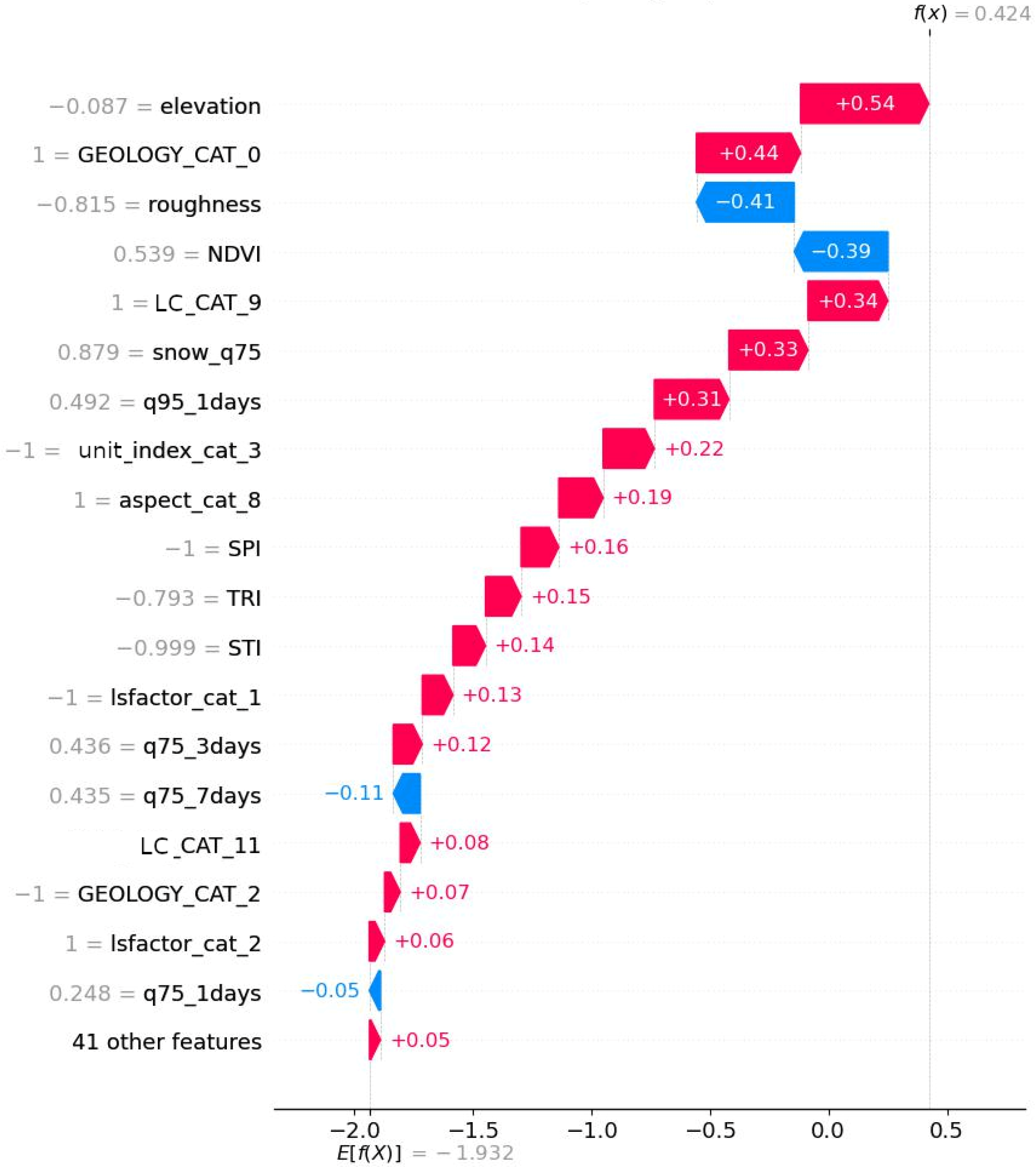
This dataset split was used to showcase the negative effect of spatial autocorrelation if left unaddressed. For this purpose, two models were trained: one using the dataset without applying the 300 m buffer (unbuffered) and one applying the buffer (buffered). As shown in Table 4, the model that used the “unbuffered” dataset for training and validation performs significantly worse in all metrics (e.g., recall 14% less; MCC less than half) compared to the model that used the “buffered” dataset, even though the latter had a smaller training set. This demonstrates that the model trained with the spatial correlation handled by the buffer filter has far better generalization capabilities.

3.3. SHAP Analysis

To gain deeper insight into the relationship between landslide causal factors and their influence on the model’s predictions, a SHAP (SHapley Additive exPlanations) analysis was conducted. This method provides a detailed, interpretable breakdown of each feature’s contribution to individual predictions, allowing for a better understanding of how different factors impact the model’s output and helping to identify key drivers of landslide susceptibility. SHAP is a powerful framework for generating local explanations, i.e., identifying what features most influenced the model’s positive or negative decisions for specific samples or groups of samples. Furthermore, the SHAP framework includes the implementation of Tree SHAP, a highly efficient explainability algorithm that is specifically designed for tree-based machine learning algorithms [66]. For this purpose, landslide points, which were located in all three units (Pindos, Gavrovo, Ionian), were selected (Figure 10). Specifically, landslides from the test dataset that were correctly predicted by the model, trained on the filtered dataset, as landslide locations were selected based on specific criteria (Table 5). In all three geotectonic units, LS points with the same slope and geology were identified (Table 5). Also, similar values for aspect and land cover were added to the selection criteria. For the selected landslides, waterfall plots were generated (Figure 11, Figure 12 and Figure 13). In the waterfall plots, the positive contribution of a feature in the characterization of a point as a landslide is represented with red and negative with blue. Axis x in the waterfall plot begins at the model’s expected output value. Each row represents how a feature’s positive or negative impact shifts the value from the expected model output (over the background dataset) to the final model output for the specific prediction.
Based on the waterfall plots (Figure 11, Figure 12 and Figure 13) generated for the points located in all three units, precipitation and geology, as expected, are the factors that positively affected the characterization of these points as possible landslide locations. In the selected geotectonic units in Greece, precipitation is the most dominant landslide-triggering factor. Also, because of the fact that all three selected predicted landslides belong to the flysch geological formation, the geology of these points positively affects the decision of the model. The flysch formation, compared to the other geological formations that exist in the area of interest (AOI) (See Table A3), is more susceptible to sliding movements. Category 4 of this aspect, as presented in Table A2, corresponds to the slopes facing towards the east. In Western Greece, where the AOI is situated, the highest precipitation frequency is recorded in the slopes facing towards the west. As a result, in Figure 11 of the point located on a slope with a west aspect (aspect_cat_7, See Table A2), the aspect has a positive impact on the characterization of this point as a landslide. In Figure 11, a correlation between elevation and snowmelt is identified. Higher snowmelt appears in higher elevation values. In the correlation matrix of Figure S1 (Supplemental Materials), a correlation between snowmelt and elevation can also be identified.
Also, in Figure 13, the selected landslide located in the Pindos unit is positively affected by aspect, identified to be West-category 8 (See Table A2). As indicated above, in Western Greece, the highest precipitation frequency is recorded on the western-facing slopes. Therefore, it is highly expected to have more intensive instability phenomena on those slopes. Summarizing, the causal factors that based on the SHAP analysis positively affect the decision of the model in landslide susceptibility are presented in Figure A1, Figure A2, Figure A3, Figure A4, Figure A5 and Figure A6 of Appendix B.

4. Discussion

ML-based landslide susceptibility mapping research was conducted, which integrates the geotectonic units in Greece and incorporates an extremely large landslide dataset derived from InSAR observations and field inspections. Landslide locations derived from the LOS displacements from the Greece InSAR product [47], validated by geotechnical experts, formed a dataset of over 3000 landslides. The detected landslides are located in three geotectonic units in Greece such as those of Pindos, Gavrovo, and Ionian. A gradient-boosted decision tree model was selected for landslide susceptibility mapping. A buffer filter was applied to the dataset to mitigate spatial autocorrelation. This methodology resulted in a model with strong generalization capabilities. The effectiveness of this method was tested by extending the model’s predictions to unseen areas, such as the Arta, Trikala, and Karditsa prefectures examined in this study. The model performed well with a precision of 79%, a recall of 73% in predicting landslide occurrences, and F1 scores of 0.89 for non-landslide events and 0.76 for landslide events. To ensure that the model’s predictions align with domain-expert knowledge, a SHAP analysis was conducted. The SHAP analysis confirmed precipitation and geology as key landslide causal factors in the investigation area.
The innovative aspects of this research are summarized as follows: (a) an exceptionally large dataset for landslide susceptibility mapping in Western Greece was created; (b) spatial autocorrelation was addressed for the first time in ML landslide susceptibility mapping; and (c) the model was successfully trained to incorporate and identify the differences in the landslide susceptibility of formations located in different geotectonic units while the geotectonic unit was introduced as a model parameter and investigated.
The landslide inventory of more than 3000 landslides, validated by ground truth and remote sensing techniques, created in the present study is an extremely big dataset compared to previous studies in the investigated prefectures of Evritania and Aitoloakarnania [6,67]. In Kontoes et al. [6], 642 landslides were also detected, including landslides derived by InSAR LOS displacements, while in [67], 92 failures were recorded through ground truth investigations. The exploitation of PSI, as presented in the current study but also in Kontoes et al. [6], highlights the efficiency of InSAR in landslide susceptibility studies. Specifically, SAR data are used for enriching landslide inventory, but they can also serve as a validation for the model’s predictions. ML is used for the first time to perform landslide susceptibility mapping in the study area. In Kontoes et al. [6], a comparison between the weights of evidence (WoE) and the Norwegian Geological Institute (NGI) methods is performed, proving that the first method is the more accurate one in landslide susceptibility mapping. In [67], the Analytical Hierarchy Process (AHP) and the Rock Engineering System (RES) methods were compared, and the second one proved more efficient in landslide predictions. Regarding similar regions in Western Greece, Bathrellos et al. [68] employed geographical information systems (GISs) and statistical spatial analysis to investigate the relationship between the landslide causal factors and landslide occurrence in Western Peloponnese in Greece.
Regarding the ML methodology, an XGBoost model was trained to predict landslide susceptibility, and a SHAP analysis was employed to validate the model’s predictions compared to the domain-specific knowledge. As expected, the SHAP analysis presented that precipitation and geology positively affected landslide characterization. As analytically described in Section 2.2 and Section 2.4, a buffer filter was applied to the dataset to mitigate spatial autocorrelation. In several ML landslide susceptibility studies [22,31,32,33,34], this effect is undervalued, leading to poor generalizability of the model. The proposed approach for spatial autocorrelation mitigation enhances the model’s generalization and establishes a strong base for developing a nationwide landslide susceptibility mapping system.
Based on the model’s predictions presented in the susceptibility map of Figure 9, the areas shown in red, which correspond to the model’s score between 0.7 and 1, are considered highly susceptible landslides. The grid created for the model’s predictions, with a cell size of 25 m, consists of 33,746,584 points in total. Among these points, 2,050,717 are located in the Pindos unit, 1,578,546 are located in the Gavrovo unit, and 1,007,408 are in the Ionios unit and have a high landslide susceptibility score between 0.7–1 (Table 6). The model’s predictions in regard to the frequency of the landslide events in each of the geotectonic units of the AOI are clearly presented in Table 6, and they appear to be aligned with the expected frequency of landslides, as indicated by former inventory studies [1]. Specifically, according to Koukis et al. [1], based on the results of a systematic inventory of data concerning landslides and their quantitative expression in Greece, the geotectonic unit of Pindos exhibits the highest frequency of landslide, exceeding 40% of the total cases recorded. The Gavrovo and Ionios geotectonic units, on the contrary, exhibit a substantially lower landslide frequency.
According to Koukis et al. [1], the most critical landslide-prone geological formation regarding lithology and structure is flysch, with a 30% frequency of recorded landslide events throughout the whole country. Also, according to the same study [1], the estimated relative frequency of landslide occurrences (with the frequency normalized to the real area covered by each lithological type) shows that although flysch predominates over the other geological formations, schist -cherts contribute significantly to the recorded landslide phenomena and they do not exceed the frequency of landslide occurrences of flysch only because they cover a small area of the country. The results of the model are in perfect agreement with the above described as, according to Table 7, although flysch formation concentrates the majority of the LS susceptible points, schist-cherts present the highest relative frequency (LS susceptible points/km2) despite their limited range on the AOI.
The promising results of this work pave the way for expanding the dataset spatially to cover more regions of the country and incorporate additional landslide-influencing factors. Advanced machine learning and deep learning methods, with various problem formulations, will be applied as part of future work, using this enriched dataset to gain deeper insights into landslides.

5. Conclusions

The proposed landslide susceptibility mapping approach that integrates InSAR with machine learning techniques demonstrates exceptional performance. By leveraging geotectonic-specific adaptations and the precision of InSAR data, combined with the predictive power of machine learning, this methodology enhances the accuracy and reliability of landslide susceptibility assessments across diverse geological contexts.
The employed XGBoost algorithm demonstrated high performance in landslide susceptibility mapping, while the SHAP analysis identified the primary triggering and preparatory factors of landslides in the investigated area. The handling of the spatial autocorrelation with a buffer filter led to a model with improved generalization ability. Leveraging the unique features of the geological formations, improved accuracy was achieved in the final ML susceptibility mapping. Particularly, the model managed to successfully incorporate the differences in the landslide susceptibility of formations located in different geotectonic units with variant geotechnical characteristics.

Supplementary Materials

The following supporting information can be downloaded at: https://www.mdpi.com/article/10.3390/rs17071161/s1, Figure S1: Pearson’s correlation matrix.

Author Contributions

Conceptualization, S.A. and C.L.; methodology, S.A., A.A., and C.L.; validation, C.L.; formal analysis, S.A. and G.C.; data curation, S.A., G.C., M.K., A.A., and N.S.B.; writing—original draft preparation, S.A.; writing—review and editing, S.A., A.A., M.K., N.S.B., G.C., C.L., and C.K.; visualization, S.A.; supervision, C.L. and C.K. All authors have read and agreed to the published version of the manuscript.

Funding

This research received no external funding.

Data Availability Statement

A minimal dataset is available on request from the corresponding author.

Acknowledgments

The authors acknowledge the Operational Unit BEYOND Centre for Earth Observation Research and Satellite Remote Sensing IAASARS/NOA for the provision of data from the InSAR Greece project and the use of the P-PSI processing chain for InSAR processing.

Conflicts of Interest

The authors declare no conflicts of interest.

Appendix A

Table A1. Slope classes.
Slope ValueClassModel Feature
0 ≤ x ≤ 20°1slope_cat_1
20° < x ≤ 40°2slope_cat_2
40° < x ≤ 60°3slope_cat_3
60° < x ≤ 80°4slope_cat_4
80° < x5slope_cat_5
Table A2. Aspect classes.
Aspect ValueClassAspect of ElevationModel Feature
x = −11Flataspect_cat_1
0° ≤ x ≤ 22.5°2Northaspect_cat_2
22.5° < x ≤ 67.5°3Northeastaspect_cat_3
67.5° < x ≤ 112.5°4Eastaspect_cat_4
112.5° < x ≤ 157.5°5Southeastaspect_cat_5
157.5° < x ≤ 202.5°6Southaspect_cat_6
202.5° < x ≤ 247.5°7Southwestaspect_cat_7
247.5° < x ≤ 292.5°8Westaspect_cat_8
292.5° < x ≤ 337.5°9Northwestaspect_cat_9
337.5° < x ≤ 360°2Northaspect_cat_2
Table A3. Geology classes.
Geology CategoryClass Model Feature
Flysch0GEOLOGY_CAT_0
Alluvial deposits1GEOLOGY_CAT_1
Limestones2GEOLOGY_CAT_2
Fine-grained igneous rock Mesozoic3GEOLOGY_CAT_3
Schist-Cherts4GEOLOGY_CAT_4
Table A4. LS factor classes.
LS FactorClassModel Feature
0 ≤ x ≤ 41lsfactor_cat_1
5 ≤ x ≤ 82lsfactor_cat_2
9 ≤ x ≤ 123lsfactor_cat_3
13 ≤ x ≤ 164lsfactor_cat_4
17 ≤ x ≤ 205lsfactor_cat_5
21 ≤ x ≤ 246lsfactor_cat_6
25 ≤ x ≤ 287lsfactor_cat_7
29 ≤ x8lsfactor_cat_8
Table A5. Classification of Corine LU/LC for the AOI.
Corine LU/LC Level 2Code 1Model Feature
Heterogeneous agricultural areas9LC_CAT_9
Forests10LC_CAT_10
Open spaces with little or no vegetation13LC_CAT_13
Scrub and/or herbaceous vegetation associations11LC_CAT_11
Pastures8LC_CAT_8
Water bodies16LC_CAT_16
Non-irrigated arable land4LC_CAT_4
Industrial, commercial, and transport units1LC_CAT_1
Permanently irrigated land5LC_CAT_5
Permanent crops7LC_CAT_7
Urban fabric0LC_CAT_0
Inland wetlands14LC_CAT_14
Mine, dump, and construction sites3LC_CAT_3
Coastal wetlands15LC_CAT_15
Rice fields6LC_CAT_6
1 Code numbers represent existing categories in the specific region.
Table A6. Geotectonic Unit Index.
Geotectonic UnitCategory 1Model Feature
Gavrovo2unit_index_cat_2
Ionios3unit_index_cat_3
Pindos8unit_index_cat_8
1 Category numbers represent existing geotectonic units in the specific region.

Appendix B

Figure A1. Aspect.
Figure A1. Aspect.
Remotesensing 17 01161 g0a1
Figure A2. Elevation.
Remotesensing 17 01161 g0a2
Figure A3. Corine land use/land cover.
Remotesensing 17 01161 g0a3
Figure A4. NDVI.
Figure A4. NDVI.
Remotesensing 17 01161 g0a4
Figure A5. Precipitation.
Remotesensing 17 01161 g0a5
Figure A6. Surface lithology.
Remotesensing 17 01161 g0a6

References

  1. Koukis, G.; Sabatakakis, N.; Nikolaou, N.; Loupasakis, C. Landslide hazard zonation in Greece. In Landslides; Springer: Berlin/Heidelberg, Germany, 2005; pp. 291–296. [Google Scholar]
  2. Koukouvelas, I.; Nikolakopoulos, K.; Zygouri, V.; Kyriou, A. Post-seismic monitoring of cliff mass wasting using an unmanned aerial vehicle and field data at Egremni, Lefkada Island, Greece. Geomorphology 2020, 367, 107306. [Google Scholar] [CrossRef]
  3. El Kamali, M.; Papoutsis, I.; Loupasakis, C.; Abuelgasim, A.; Omari, K.; Kontoes, C. Monitoring of land surface subsidence using persistent scatterer interferometry techniques and ground truth data in arid and semi-arid regions, the case of Remah, UAE. Sci. Total Environ. 2021, 776, 145946. [Google Scholar] [CrossRef] [PubMed]
  4. Alatza, S.; Papoutsis, I.; Paradissis, D.; Kontoes, C.; Papadopoulos, G.A. Multi-Temporal InSAR Analysis for Monitoring Ground Deformation in Amorgos Island, Greece. Sensors 2020, 20, 338. [Google Scholar] [CrossRef]
  5. Sykioti, O.; Kontoes, C.; Elias, P.; Briole, P.; Sachpazi, M.; Paradissis, D.; Kotsis, I. Ground deformation at Nisyros volcano (Greece) detected by ERS-2 SAR differential interferometry. Int. J. Remote Sens. 2003, 24, 183–188. [Google Scholar] [CrossRef]
  6. Kontoes, C.; Loupasakis, C.; Papoutsis, I.; Alatza, S.; Poyiadji, E.; Ganas, A.; Psychogyiou, C.; Kaskara, M.; Antoniadi, S.; Spanou, N. Landslide Susceptibility Mapping of Central and Western Greece, Combining NGI and WoE Methods, with Remote Sensing and Ground Truth Data. Land 2021, 10, 402. [Google Scholar] [CrossRef]
  7. Nefros, C.; Alatza, S.; Loupasakis, C.; Kontoes, C. Persistent Scatterer Interferometry (PSI) Technique for the Identification and Moni-toring of Critical Landslide Areas in a Regional and Mountainous Road Network. Remote Sens. 2023, 15, 1550. [Google Scholar] [CrossRef]
  8. Aslan, G.; Foumelis, M.; Raucoules, D.; De Michele, M.; Bernardie, S.; Cakir, Z. Landslide Inventory Mapping and Monitoring Using Persistent Scatterer Interferometry (PSI) Technique in the French Alps. Remote Sens. 2020, 12, 1305. [Google Scholar] [CrossRef]
  9. Jia, H.; Wang, Y.; Ge, D.; Deng, Y.; Wang, R. InSAR Study of Landslides: Early Detection, Three-Dimensional, and Long-Term Surface Displacement Estimation—A Case of Xiaojiang River Basin, China. Remote Sens. 2022, 14, 1759. [Google Scholar] [CrossRef]
  10. Ohki, M.; Abe, T.; Tadono, T.; Shimada, M. Landslide detection in mountainous forest areas using polarimetry and interferometric coherence. Earth Planets Space 2020, 72, 67. [Google Scholar] [CrossRef]
  11. Tzouvaras, M.; Danezis, C.; Hadjimitsis, D.G. Small Scale Landslide Detection Using Sentinel-1 Interferometric SAR Coherence. Remote Sens. 2020, 12, 1560. [Google Scholar] [CrossRef]
  12. Ma, P.; Cui, Y.; Wang, W.; Lin, H.; Zhang, Y.; Zheng, Y. Landslide Movement Monitoring with InSAR Technologies. In Landslides; IntechOpen: London, UK, 2022. [Google Scholar] [CrossRef]
  13. Hussain, S.; Pan, B.; Afzal, Z.; Ali, M.; Zhang, X.; Shi, X.; Ali, M. Landslide detection and inventory updating using the time-series InSAR approach along the Karakoram Highway, Northern Pakistan. Sci. Rep. 2023, 13, 7485. [Google Scholar] [CrossRef]
  14. Smail, T.; Abed, M.; Mebarki, A.; Lazecky, M. Earthquake-induced landslide monitoring and survey by means of InSAR. Nat. Hazards Earth Syst. Sci. 2022, 22, 1609–1625. [Google Scholar] [CrossRef]
  15. Bekaert, D.P.S.; Handwerger, A.L.; Agram, P.; Kirschbaum, D.B. InSAR-based detection method for mapping and monitoring slow-moving landslides in remote regions with steep and mountainous terrain: An application to Nepal. Remote Sens. Environ. 2020, 249, 111983. [Google Scholar] [CrossRef]
  16. Jia, H.; Wang, Y.; Ge, D.; Deng, Y.; Wang, R. Insar Driven Landslide Detection and Monitoring Based on Small Baseline Sets: A Case Study of Jinsha River Valley (Dongchuan Section). In Proceedings of the 2021 IEEE International Geoscience and Remote Sensing Symposium IGARSS, Brussels, Belgium, 11–16 July 2021; pp. 8388–8391. [Google Scholar] [CrossRef]
  17. Ma, Z.; Mei, G.; Piccialli, F. Machine learning for landslides prevention: A survey. Neural Comput. Appl. 2021, 33, 10881–10907. [Google Scholar] [CrossRef]
  18. Ballabio, C.; Sterlacchini, S. Support Vector Machines for Landslide Susceptibility Mapping: The Staffora River Basin Case Study, Italy. Math. Geosci. 2012, 44, 47–70. [Google Scholar] [CrossRef]
  19. Lee, S.; Hong, S.-M.; Jung, H.-S. A Support Vector Machine for Landslide Susceptibility Mapping in Gangwon Province, Ko-rea. Sustainability 2017, 9, 48. [Google Scholar] [CrossRef]
  20. Xu, K.; Zhao, Z.; Chen, W.; Ma, J.; Liu, F.; Zhang, Y.; Ren, Z. Comparative study on landslide susceptibility mapping based on different ratios of training samples and testing samples by using RF and FR-RF models. Nat. Hazards Res. 2024, 4, 62–74. [Google Scholar] [CrossRef]
  21. Park, S.; Kim, J. Landslide Susceptibility Mapping Based on Random Forest and Boosted Regression Tree Models, and a Comparison of Their Performance. Appl. Sci. 2019, 9, 942. [Google Scholar] [CrossRef]
  22. Can, R.; Kocaman, S.; Gokceoglu, C. A Comprehensive Assessment of XGBoost Algorithm for Landslide Susceptibility Mapping in the Upper Basin of Ataturk Dam, Turkey. Appl. Sci. 2021, 11, 4993. [Google Scholar] [CrossRef]
  23. Badola, S.; Varun, M.; Surya, P. Landslide susceptibility mapping using XGBoost machine learning method. In Proceedings of the 2023 International Conference on Machine Intelligence for GeoAnalytics and Remote Sensing (MIGARS), Hyderabad, India, 27–29 January 2023; pp. 1–4. [Google Scholar] [CrossRef]
  24. Hussain, M.A.; Chen, Z.; Zheng, Y.; Shoaib, M.; Shah, S.U.; Ali, N.; Afzal, Z. Landslide Susceptibility Mapping Using Machine Learning Algorithm Validated by Persistent Scatterer In-SAR Technique. Sensors 2022, 22, 3119. [Google Scholar] [CrossRef]
  25. Kavzoglu, T.; Teke, A. Predictive Performances of Ensemble Machine Learning Algorithms in Landslide Susceptibility Mapping Using Random Forest, Extreme Gradient Boosting (XGBoost) and Natural Gradient Boosting (NGBoost). Arab. J. Sci. Eng. 2022, 47, 7367–7385. [Google Scholar] [CrossRef]
  26. Sahin, E.K. Comparative analysis of gradient boosting algorithms for landslide susceptibility mapping. Geocarto Int. 2020, 37, 2441–2465. [Google Scholar] [CrossRef]
  27. Karantanellis, E.; Marinos, V.; Vassilakis, E.; Hölbling, D. Evaluation of Machine Learning Algorithms for Object-Based Mapping of Landslide Zones Using UAV Data. Geosciences 2021, 11, 305. [Google Scholar] [CrossRef]
  28. Ferreira, Z.; Almeida, B.; Costa, A.C.; do Couto Fernandes, M.; Cabral, P. Insights into landslide susceptibility: A comparative evaluation of multi-criteria analysis and machine learning techniques. Geomatics. Nat. Hazards Risk 2025, 16, 2471019. [Google Scholar] [CrossRef]
  29. Ngo, P.T.T.; Panahi, M.; Khosravi, K.; Ghorbanzadeh, O.; Kariminejad, N.; Cerda, A.; Lee, S. Evaluation of deep learning algorithms for national scale landslide susceptibility mapping of Iran. Geosci. Front. 2021, 12, 505–519. [Google Scholar] [CrossRef]
  30. Azarafza, M.; Azarafza, M.; Akgün, H.; Atkinson, P.M.; Derakhshani, R. Deep learning-based landslide susceptibility mapping. Sci. Rep. 2021, 11, 24112. [Google Scholar] [CrossRef] [PubMed]
  31. Dahim, M.; Alqadhi, S.; Mallick, J. Enhancing landslide management with hyper-tuned machine learning and deep learning models: Predicting susceptibility and analyzing sensitivity and uncertainty. Front. Ecol. Evol. 2023, 11, 1108924. [Google Scholar] [CrossRef]
  32. Kainthura, P.; Sharma, N. Hybrid machine learning approach for landslide prediction, Uttarakhand, India. Sci. Rep. 2022, 12, 20101. [Google Scholar] [CrossRef]
  33. Sheng, M.; Zhou, J.; Chen, X.; Teng, Y.; Hong, A.; Liu, G. Landslide Susceptibility Prediction Based on Frequency Ratio Method and C5.0 Decision Tree Model. Front. Earth Sci. 2022, 10, 918386. [Google Scholar] [CrossRef]
  34. Nhu, V.-H.; Mohammadi, A.; Shahabi, H.; Ahmad, B.B.; Al-Ansari, N.; Shirzadi, A.; Clague, J.J.; Jaafari, A.; Chen, W.; Nguyen, H. Landslide Susceptibility Mapping Using Machine Learning Algorithms and Remote Sensing Data in a Tropical Environment. Int. J. Environ. Res. Public Health 2020, 17, 4933. [Google Scholar] [CrossRef]
  35. Nikparvar, B.; Thill, J.-C. Machine Learning of Spatial Data. ISPRS Int. J. Geo-Inf. 2021, 10, 600. [Google Scholar] [CrossRef]
  36. Apostolakis, A.; Girtsou, S.; Giannopoulos, G.; Bartsotas, N.S.; Kontoes, C. Estimating Next Day’s Forest Fire Risk via a Complete Machine Learning Methodology. Remote Sens. 2022, 14, 1222. [Google Scholar] [CrossRef]
  37. Sabatakakis, N.; Koukis, G.; Vassiliades, E.; Lainas, S. Landslide susceptibility zonation in Greece. Nat. Hazards 2013, 65, 523–543. [Google Scholar]
  38. Kilias, A. The Hellenides: A multiphase deformed orogenic belt, its structural architecture, kinematics and geotectonic setting during the Alpine orogeny: Comression vs Extension the dynamic peer for the orogen making. A synthesis. J. Geol. Geosci. 2021, 15, 2021. [Google Scholar]
  39. Mountrakis, D.; Sapountzis, E.; Kilias, A.; Elefteriadis, G.; Christofides, G. Paleogeographic conditions in the western Pelagonian margin in Greece during the initial rifting of the continental area. Can. J. Earth Sci. 1983, 20, 1673–1681. [Google Scholar]
  40. Mountrakis, D. Γεωλογια και Γεωτεκτονικη Εξελιξη της Ελλαδας; University Studio Press: Thessaloniki, Greece, 2010; p. 374. [Google Scholar]
  41. Doutsos, T.; Kokkalas, S. Stress and deformation patterns in the Aegean region. J. Struct. Geol. 2001, 23, 455–472. [Google Scholar]
  42. Kassaras, I. Study of the geodynamics in Aitoloakarnania (W. Greece) based on joint seismological and GPS data. In Proceedings of the 33rd ESC General Assembly, Moscow, Russia, 19–24 August 2012. [Google Scholar]
  43. Dermitzakis, M.D.; Papanikolaou, D.J. Paleogeography and geodynamics of the Aegean region during the Neogene. Ann. Geol. Pays Hell. 1981, 30, 245–289. [Google Scholar]
  44. Koukouvelas, I.; Aydin, A. Fault structure and related basins of the North Aegean Sea and its surroundings. Tectonics 2002, 21, 10-1–10-17. [Google Scholar]
  45. Marinos, V.; Papathanassiou, G.; Vougiouka, E.; Karantanellis, E. Towards the Evaluation of Landslide Hazard in the Mountainous Area of Evritania, Central Greece. In Engineering Geology for Society and Territory—Volume 2; Lollino, G., Giordan, D., Crosta, G.B., Corominas, J., Azzam, R., Wasowski, J., Sciarra, N., Eds.; Springer: Cham, Switzerland, 2015; pp. 989–993. [Google Scholar]
  46. Delibasis, N.; Karydis, P. Recent earthquake activity in Trichonis region and its tectonic significance. Ann. Geophys. 1977, 30, 19–81. [Google Scholar]
  47. Papoutsis, I.; Kontoes, C.; Alatza, S.; Apostolakis, A.; Loupasakis, C. InSAR Greece with Parallelized Persistent Scatterer Interferometry: A National Ground Motion Service for Big Copernicus Sentinel-1 Data. Remote Sens. 2020, 12, 3207. [Google Scholar] [CrossRef]
  48. Hooper, A.; Zebker, H.; Segall, P.; Kampes, B. A new method for measuring deformation on volcanoes and other natural terrains using InSAR persistent scatterers. Geophys. Res. Lett. 2004, 31, L23611. [Google Scholar] [CrossRef]
  49. Skilodimou, H.D.; Bathrellos, G.D.; Koskeridou, E.; Soukis, K.; Rozos, D. Physical and Anthropogenic Factors Related to Landslide Activity in the Northern Peloponnese, Greece. Land 2018, 7, 85. [Google Scholar] [CrossRef]
  50. Papathanassiou, G.; Valkaniotis, S.; Ganas, A. Spatial patterns, controlling factors, and characteristics of landslides triggered by strike-slip faulting earthquakes: Case study of Lefkada island, Greece. Bull. Eng. Geol. Environ. 2021, 80, 3747–3765. [Google Scholar] [CrossRef]
  51. Nefros, C.; Tsagkas, D.S.; Kitsara, G.; Loupasakis, C.; Giannakopoulos, C. Landslide Susceptibility Mapping under the Climate Change Impact in the Chania Regional Unit, West Crete, Greece. Land 2023, 12, 154. [Google Scholar] [CrossRef]
  52. Argyriou, A.V.; Polykretis, C.; Teeuw, R.M.; Papadopoulos, N. Geoinformatic Analysis of Rainfall-Triggered Landslides in Crete (Greece) Based on Spatial Detection and Hazard Mapping. Sustainability 2022, 14, 3956. [Google Scholar] [CrossRef]
  53. Hellenic National Meteorological Service (HNMS). Climate Atlas of Greece 1971–2000. 2016. Available online: http://climatlas.hnms.gr/sdi/ (accessed on 8 March 2025).
  54. Clerici, A.; Perego, S.; Tellini, C.; Vescovi, P. A GIS-based automated procedure for landslide susceptibility mapping by the Conditional Analysis method: The Baganza valley case study (Italian Northern Apennines). Environ. Geol. 2006, 50, 941–961. [Google Scholar] [CrossRef]
  55. Meten, M.; PrakashBhandary, N.; Yatabe, R. Effect of Landslide Factor Combinations on the Prediction Accuracy of Landslide Susceptibility Maps in the Blue Nile Gorge of Central Ethiopia. Geoenviron. Disasters 2015, 2, 9. [Google Scholar] [CrossRef]
  56. Wischmeier, W.H.; Smith, D.D. Predicting Rainfall Erosion Losses; Agriculture Handbook, n. 537, Agriculture Research Service; US Department of Agriculture: Washington, DC, USA, 1978.
  57. Henriques, C.; Zêzere, J.; Marques, F. The role of the lithological setting on the landslide pattern and distribution. Eng. Geol. 2015, 189, 17–31. [Google Scholar] [CrossRef]
  58. Peduzzi, P. Landslides and vegetation cover in the 2005 North Pakistan earthquake: A GIS and statistical quantitative approach. Nat. Hazards Earth Syst. Sci. 2010, 10, 623–640. [Google Scholar] [CrossRef]
  59. Digital Elevation Model over Europe (EU-DEM). Available online: https://www.eea.europa.eu/data-and-maps/data/eu-dem (accessed on 25 November 2024).
  60. LS-Factor (Slope Length and Steepness Factor) for the EU. Available online: https://esdac.jrc.ec.europa.eu/content/ls-factor-slope-length-and-steepness-factor-eu (accessed on 3 November 2023).
  61. Copernicus Corine Land Cover 2018. Available online: https://land.copernicus.eu/en/products/corine-land-cover/clc2018 (accessed on 25 November 2024).
  62. EGDI 1:1 Million Pan-European Surface Geology. Available online: https://egdi.geology.cz/record/basic/5f7db57f-6e84-4484-835f-706b0a010833 (accessed on 3 November 2023).
  63. ERA5-Land Hourly Data from 1950 to Present. Available online: https://cds.climate.copernicus.eu/cdsapp#!/dataset/reanalysis-era5-land?tab=overview (accessed on 25 November 2024).
  64. Gorelick, N.; Hancher, M.; Dixon, M.; Ilyushchenko, S.; Thau, D.; Moore, R. Google Earth Engine: Planetary-scale geospatial analysis for everyone. Remote Sens. Environ. 2017, 202, 18–27. [Google Scholar]
  65. Chicco, D.; Jurman, G. The advantages of the Matthews correlation coefficient (MCC) over F1 score and accuracy in binary classification evaluation. BMC Genom. 2020, 21, 6. [Google Scholar] [CrossRef]
  66. Lundberg, S.M.; Erion, G.; Chen, H.; DeGrave, A.; Prutkin, J.M.; Nair, B.; Katz, R.; Himmelfarb, J.; Bansal, N.; Lee, S.I. From local explanations to global understanding with explainable AI for trees. Nat. Mach. Intell. 2020, 2, 56–67. [Google Scholar] [CrossRef] [PubMed]
  67. Krassakis, P.; Ioannidou, A.; Tsangaratos, P.; Loupasakis, C. Landslide Susceptibility Mapping of the Aitoloakarnania and Evrytania regional units, Western Greece, updated with the extensive catastrophic of Winter 2015. In Proceedings of the ICED2020: 1st International Conference on Environmental Design, Athens, Greece, 24–25 October 2020. [Google Scholar] [CrossRef]
  68. Bathrellos, G.; Koukouvelas, I.; Skilodimou, H.; Nikolakopoulos, K.; Vgenopoulos, A. Landslide causative factors evaluation using GIS in the tectonically active Glafkos River area, northwestern Peloponnese, Greece. Geomorphology 2024, 461, 109285. [Google Scholar] [CrossRef]
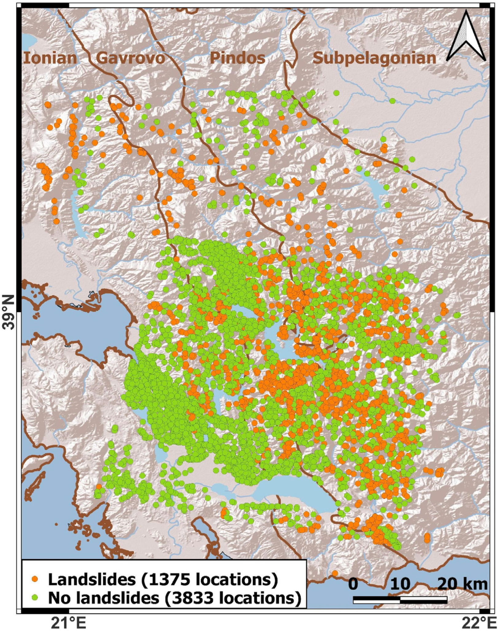
Figure 1. The study area depicted with the orange rectangle and the investigated prefectures in Greece.
Remotesensing 17 01161 g001
Figure 2. The study area and the geotectonic units of Greece.
Remotesensing 17 01161 g002
Figure 3. Landslide inventory used in the ML landslide susceptibility model.
Remotesensing 17 01161 g003
Figure 4. Indicative examples of slope failures in the Evritania and Aitoloakarnania prefectures used for the verification of the landslide dataset. The slope failures at (a) Prousos, (b) Klepa, (c) Nerosirtis, and (d) Kokkinovrisi.
Remotesensing 17 01161 g004
Figure 5. Landslide dataset used in the ML landslide susceptibility model.
Remotesensing 17 01161 g005
Figure 6. Methodology workflow.
Remotesensing 17 01161 g006
Figure 7. Train/validation test set split settings: (a) the main setting, where the training/validation dataset area overlaps with the test dataset area; (b) the test dataset is located in a remote area, with practically no spatial correlation between the two sets.
Remotesensing 17 01161 g007
Figure 8. Confusion matrix.
Remotesensing 17 01161 g008
Figure 9. Landslide susceptibility map. The landslide locations of the test dataset are also added as an indicator of the model’s performance.
Remotesensing 17 01161 g009
Figure 10. Landslides selected for SHAP analysis.
Remotesensing 17 01161 g010
Figure 11. Waterfall plot for the Gavrovo unit landslide of case 1. The meanings of the abbreviations located on the Y-axis can be found in the tables of Appendix A.
Remotesensing 17 01161 g011
Figure 12. Waterfall plot for the Ionian unit landslide. The meanings of the abbreviations located on the Y-axis can be found in the tables of Appendix A.
Remotesensing 17 01161 g012
Figure 13. Waterfall plot for the Pindos unit landslide. The meanings of the abbreviations located on the Y-axis can be found in the tables of Appendix A.
Remotesensing 17 01161 g013
Table 1. The sources and total number of landslides.
No of LS PointsSource
642 Kontoes et al. [6]
704Visual inspection of satellite images
2354InSAR Greece product [47]
Table 2. Landslides triggering factors employed in the ML model.
CategoryModel ParametersFeature Code Name
GeomorphologyElevationelevation (numerical)
Roughnessroughness (numerical)
Aspectaspect (one-hot class)
Slopeslope (one-hot class)
GeologyLS factorlsfactor (one-hot class)
Surface LithologyGEOLOGY (one-hot class)
Geotectonic unitunit_index (one-hot class)
ClimateSnow melt snow_q75 (numerical)
Precipitation q95_1days, q95_3days, q95_7days, q95_30days, q75_1days, etc.
(numerical)
Hydrology and TopographySediment Transport Index STI (numerical)
Topographic Wetness IndexTWI (numerical)
Terrain Ruggedness IndexTRI (numerical)
Stream Power IndexSPI (numerical)
VegetationNormalized Difference
Vegetation Index
NDVI (numerical)
Land use–Land coverLand use–Land coverLC (one-hot class)
Table 3. XGBoost classification report.
Score MetricPrecisionRecallF1SupportAccuracyMCC
No Landslide0.880.910.898270.850.65
Landslide0.790.730.76392
Table 4. XGBoost classification report of the model using the “buffered” and “unbuffered” datasets for training and validation.
DatasetScore MetricPrecisionRecallF1AccuracyMCC
BufferedNo Landslide0.730.460.560.710.38
Landslide0.700.880.78
UnbufferedNo Landslide0.670.430.530.570.17
Landslide0.510.740.60
Table 5. Selection criteria for LS points for SHAP analysis.
LS PointsAspect
(Degrees)
Slope
(Degrees)
Geology Land Use/Land Cover
LS Ionios 157.5–202.50–20FlyschHeterogeneous agricultural areas
LS Gavrovo202.5–247.50–20FlyschScrub and/or herbaceous vegetation associations
LS Pindos247.5–292.50–20FlyschHeterogeneous agricultural areas
Table 6. The percentage of highly susceptible landslide points calculated from the total number of the grid points in the three geotectonic units included at the AOI.
PindosGavrovoIonios
No. of the grid’s high LS susceptible points2,050,717 (44%)1,578,546 (34%)1,007,408 (22%)
Unit area within the AOI (in km2)347464906958
Grid’s high LS susceptible points/km2590243145
Table 7. The percentage of highly susceptible landslide points calculated from the total number of the grid points classified based on their geological formation in the three geotectonic units included at the AOI.
No. of the Grid’s High LS Susceptible PointsGeological Formations Area Within the AOI
(in km2)
Grid’s High LS Susceptible Points/km2
Flysch3,269,5717665426
Limestones 1,820,2705927307
Alluvial deposits299,3321842162
Schist-cherts327,211502651
Disclaimer/Publisher’s Note: The statements, opinions and data contained in all publications are solely those of the individual author(s) and contributor(s) and not of MDPI and/or the editor(s). MDPI and/or the editor(s) disclaim responsibility for any injury to people or property resulting from any ideas, methods, instructions or products referred to in the content.

