Abstract
Mapping flooded areas immediately after heavy rainfall is particularly challenging when sediment-laden floodwaters dominate the landscape. Traditional indices, such as the Normalized Difference Water Index (NDWI), are designed to detect water-covered areas but fail to identify muddy zones with high turbidity, which are common during extreme flood events. These muddy floodwaters often blend spectrally with surrounding land, leading to significant misclassifications. This study introduces the Flood Mud Index (FMI), a novel spectral index specifically developed to detect debris-laden flooded areas using only the red and blue bands. Landsat 8 imagery was utilized to validate the FMI, and its performance was evaluated through confusion matrices. The index achieved an overall accuracy of 97.86%, outperforming existing indices and demonstrating exceptional precision in delineating muddy floodplains. By relying solely on red and blue bands, the FMI is applicable to any platform equipped with RGB sensors, offering versatility for flood monitoring. Its compatibility with low-cost drones makes it especially valuable for rapid post-flood assessments, enabling immediate data collection even in scenarios with persistent cloud cover. The FMI addresses a critical gap in flood mapping, providing an effective tool for emergency response and management in sediment-rich environments.
1. Introduction
Floods occur when the flow of water exceeds the capacity of the natural or artificial systems designed to convey or contain it [1]. They can be broadly categorized into two main types: pluvial floods, caused by intense rainfall that generates excessive surface runoff and leads to a rapid rise in water levels, and fluvial floods, which result from the overflow of rivers or streams into the surrounding land [2]. Coastal flooding is another form, occurring when water levels rise significantly in coastal areas due to storm surges or tidal events [3].
Flooding ranks among the most devastating natural disasters, causing widespread damage to lives, livelihoods, and infrastructure [4,5]. Over the years, the frequency and intensity of floods have increased, partly driven by climate change, which is leading to more extreme precipitation events [6]. This growing threat underscores the need for effective mitigation and emergency response strategies. According to the Directive 2007/60/EC of the European Parliament and of the Council [7], floods pose significant risks to human health, the environment, cultural heritage, and economic activities. Addressing these risks requires timely and accurate information about flood extent and impacted areas, which is critical for implementing response measures and minimizing harm during and after flood events.
Modern remote sensing technologies, such as multispectral optical sensors [8] and synthetic-aperture radar (SAR) [9], have become indispensable tools for monitoring floods. These technologies provide critical data for assessing flood extent and generating additional information products needed to guide emergency response efforts [10]. However, challenges remain in acquiring real-time data in the immediate aftermath of a flood, particularly under conditions of persistent cloud cover or when distinguishing water from sediment-laden surfaces [11,12].
Flood mapping is typically focused on the field of land cover classification and semantic segmentation within optical remote sensing [13,14,15]. One common approach involves the use of spectral indices, such as the Normalized Difference Water Index (NDWI) [16], which leverages differences in light absorption between green and near-infrared wavelengths to detect water bodies. However, the effectiveness of such indices can vary significantly depending on environmental conditions and tend to perform poorly [17,18], as the spectral properties of floodwater are often influenced by debris, pollutants, and suspended sediments [19].
The NDWI is perhaps the most widely used index in the literature for mapping flooded areas from satellite imagery [20,21,22]. However, its adoption is not universal, primarily due to the inherent limitations associated with its application. One of the most commonly used indices is the Modified Normalized Difference Water Index (MNDWI) proposed by Xu in 2006 [23]. Originally proposed for enhancing open water features, this enhanced version of the NDWI has since been adapted by various authors for flood mapping [24,25,26]. The MNDWI replaces the near-infrared (NIR) band with the shortwave infrared (SWIR) band, improving its sensitivity to water bodies. Albertini et al. [27] identified the MNDWI as the most effective index for detecting flooded areas in multispectral satellite imagery, outperforming several other indices. In addition to the MNDWI, the Automated Water Extraction Index (AWEI), introduced by Feyisa et al. in 2014 [28], is another widely used index in the literature. Designed to enhance the detection of water bodies, the AWEI is particularly effective in addressing challenges posed by shadows and dark surfaces, improving classification accuracy in such conditions. While the index generally yields reliable results [29,30], some studies have reported reduced performance in areas with dense vegetation [31] or highly turbid-muddy water [32]. The indices discussed so far were originally developed for different purposes, such as the general mapping of water bodies or coastline extraction [33,34,35]. In contrast, the Normalized Difference Flood Index (NDFI) was specifically designed to map areas affected by flooding. Introduced by Wan et al. in 2018 [36], this index utilizes blue and SWIR bands to enhance the detection of flood-impacted regions.
Most studies employing these indices rely on a bi-temporal analysis approach [37,38,39,40], comparing satellite imagery captured before and after the flooding event to identify changes indicative of flooding. This method is usually effective for detecting flood extent but requires the availability of pre-event imagery, which is not always guaranteed. However, some authors have demonstrated the feasibility of using only post-flood imagery to map flooded areas [41,42]. These approaches focus on leveraging spectral properties and advanced classification techniques to detect inundated regions without the need for pre-event baseline images, making them particularly valuable in emergency situations where pre-flood data are unavailable or compromised.
In addition to these methodologies, Linear Spectral Unmixing (LSU) has been employed in flood mapping to estimate the fractional abundance of water and other land cover types within mixed pixels. LSU decomposes each pixel’s spectral signature into a combination of endmember spectra, representing pure materials, to determine their respective proportions within the pixel [43]. This approach is particularly beneficial when dealing with coarse spatial resolution imagery, where pixels often encompass multiple land cover types [44]. For instance, in Bangira et al. [45], the authors developed and applied a new unmixing method based on the use of an ensemble of spectral endmembers (pure spectra of land cover features) to capture and take into account spectral variability within each endmember. However, the accuracy of LSU heavily depends on the precise identification of endmembers and the assumption of linear mixing, which may not always hold true in complex flood scenarios [46]. LSU is a technique commonly applied to hyperspectral images [47,48,49], as these provide high spectral resolution, which enhances the accuracy of spectral unmixing [43]. Additionally, LSU is particularly effective when distinguishing between multiple material classes within a single pixel. However, in the context of flood mapping, the primary objective is often a binary classification between flooded and non-flooded areas. In such cases, applying LSU may not offer significant advantages over more direct classification methods, as its strength lies in handling complex spectral mixtures rather than simple dichotomous separations [50].
Given the challenges associated with detecting flooded areas using traditional indices, particularly in the presence of high concentrations of suspended sediments, this paper aims to introduce a novel methodology tailored to such conditions. The proposed approach revolves around a new index specifically designed to identify areas inundated with sediment-laden floodwaters, commonly referred to as mud. This index, named the Flood Mud Index (FMI), addresses the limitations of existing methods and provides a more accurate tool for mapping muddy floodplains.
Particularly, this study focuses on the aftermath of the recent flood event that affected Valencia on 29 October 2024. The severe rainfall caused widespread inundation, with many areas heavily impacted by muddy floodwaters due to significant sediment transport. The disaster resulted in extensive damage to infrastructure and property, with over 200 lives tragically lost, underscoring the urgent need for accurate flood mapping to support effective response and recovery efforts.
All the analyses were carried out in Quantum GIS version 3.22.
2. Study Area and Dataset
Valencia, located on the eastern coast of Spain (as shown in Figure 1), lies geographically at the confluence of the Turia River to the north and the Júcar River to the south. The surrounding region is characterized by a coastal plain that extends up to 50 km inland, bordered by mountain ranges with an average elevation of 1000 m [51].
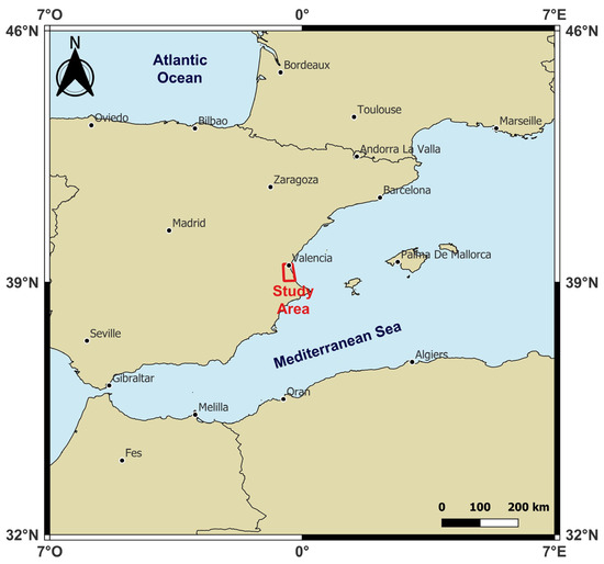
Figure 1.
Geo-localization of the study area (highlighted in red) in equirectangular projection and WGS 84 ellipsoidal coordinates (EPSG: 4326).
The Turia River spans 280 km and flows through the city of Valencia, which is home to approximately 1.4 million people. The river exhibits a variable flow regime, with a spring peak, a minimum flow in summer, a secondary low in January due to rainfall deficits, and another peak in June typically associated with convective storms [52]. Annual precipitation in the Turia River basin varies significantly, ranging from less than 400 mm to over 1000 mm, depending on the location [53]. Extreme flooding events often occur when storms with E-SE winds reach the central Turia basin, coinciding with torrential rainfall affecting the lower tributaries. This combination can lead to significant inundations on the coastal floodplain [54,55].
Additionally, Valencia’s historical irrigation system, the Horta de València, consists of extensive agricultural lands and a network of water channels [56]. While this system is vital for agricultural sustainability, it adds complexity to flood management due to its impact on regional hydrology [57,58].
The Albufera, a coastal lagoon located south of Valencia, is another critical hydrological feature of the region. This natural wetland, one of the largest in Spain, plays a significant role in the area’s water dynamics and serves as a buffer against flooding [59]. It spans an area of 23.1 km2 and has a shallow average depth of just 1 m, reaching a maximum depth of 1.6 m. The Albufera and its surrounding rice paddies are integral to the region’s agricultural [60] and ecological balance [61]. However, this delicate ecosystem is also vulnerable to extreme weather events, with torrential rains often causing water levels to rise rapidly, exacerbating flood risks in nearby areas [62,63].
The Albufera’s interaction with the Turia and Júcar river basins, as well as its proximity to densely populated areas, has been the subject of numerous studies analyzing how the lagoon contributes to flood management while also assessing the risks it faces during extreme rainfall events [64,65,66].
The Valencia region has been extensively studied from a hydrological perspective [67,68], given its susceptibility to flooding and its complex interplay of natural and human-modified systems. Numerous studies in the literature have analyzed the flood risk in the area, focusing on various factors such as rainfall patterns [69], river dynamics [70], and the impact of human interventions [71], highlighting the region’s vulnerability.
For this study, Landsat 8 satellite imagery (Level 1) acquired on October 30, 2024, was utilized. A specific area of interest was clipped from the dataset, shown in Figure 2, with the following spatial extent (UTM/WGS84–31 zone coordinate system): E1 = 196,605 m; E2 = 224,055 m, N1 = 4,326,615 m; N2 = 4,378,755 m.
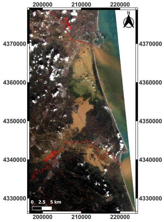
Figure 2.
RGB true color composition of the Landsat 8 OLI images in UTM/WGS 84 plane coordinates (EPSG: 32631). The Jucar and Turia rivers are highlighted in red.
The Landsat 8 satellite is equipped with two primary scientific instruments: the Operational Land Imager (OLI) and the Thermal Infrared Sensor (TIRS). These sensors collectively deliver global land coverage with varying spatial resolutions: 30 m for visible, near-infrared (NIR), and shortwave infrared (SWIR) bands; 100 m for thermal infrared; and 15 m for the panchromatic band [72]. For this study, only the bands from the Operational Land Imager (OLI) were utilized, as detailed in Table 1.

Table 1.
Characteristics of Landsat 9 OLI multispectral bands used in this study.
The Landsat 8 satellite operates in tandem with Landsat 9, forming a constellation. Both satellites are positioned in a sun-synchronous orbit at an altitude of 705 km, with an 8-day phase difference between them [73].
3. Methods
The workflow for this study (Figure 3) consisted of four main steps, following an initial preprocessing phase: mask creation, application of spectral indices, classification, and accuracy assessment.
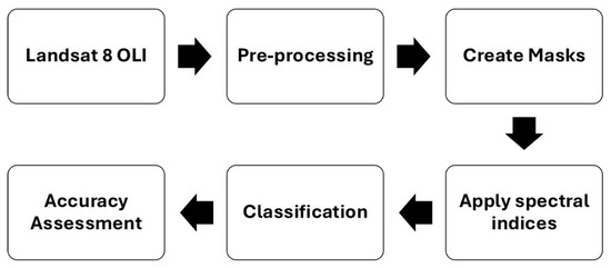
Figure 3.
Workflow of the methodology applied in this study.
3.1. Pre-Processing
To prepare the Level 1 Landsat 8 imagery for spectral analysis, pre-processing was performed to obtain surface reflectance values.
This process began with the conversion of raw digital numbers (DNs) into top-of-atmosphere (TOA) radiance, which represents the solar radiation incident on the satellite sensor, using calibration coefficients provided in the Landsat metadata file [73].
TOA reflectance, as recorded by satellite sensors, is influenced by atmospheric effects such as scattering, absorption, and emission, which modify the electromagnetic radiation as it travels through the atmosphere [74]. To mitigate these effects, atmospheric correction was applied using the Dark Object Subtraction (DOS) model [75], a widely used empirical method in remote sensing. This correction ensured that the surface reflectance data accurately represented the Earth’s surface properties and were suitable for spectral analysis.
3.2. Masking
Some preliminary operations were conducted to ensure consistent conditions across all indices. These steps were designed to focus exclusively on the relevant areas within the region of interest:
Sea Mask Creation: To exclude marine areas from the analysis, a sea mask was generated, ensuring that only terrestrial and potentially flooded zones were considered.
Cloud Mask Creation: To prevent misclassification caused by cloud cover, a cloud mask was applied to remove these areas from the investigation.
Exclusion of the Albufera Wetland and rivers: to prevent misclassification and ensure accurate results, both the Albufera Wetland and river systems within the study area were excluded from training and test site selection. The Albufera represents a distinct wetland environment [76], while rivers such as the Júcar and Turia naturally contain water year-round and are not indicative of flood-induced sediment-laden areas. To achieve this, the official shapefiles for the Albufera Natural Park [77] and the Spanish hydrographic network [78] were obtained and utilized (shown in Figure 4). No training or test sites were selected within these designated regions to avoid introducing bias into the classification process.
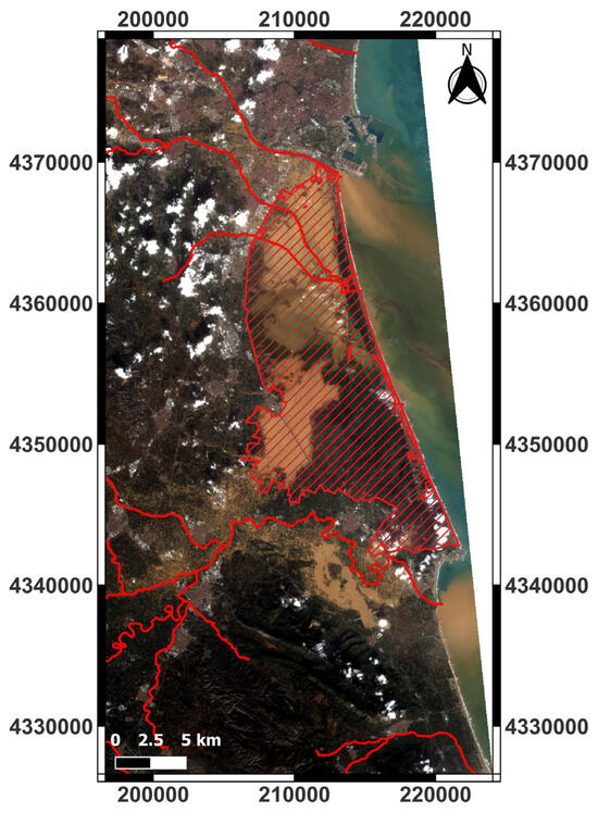
Figure 4.
Landsat 8 satellite image showing the study area near Valencia, Spain. The red outline represents the shapefile boundaries of the Albufera Natural Park (hatched area) and the major rivers, including the Júcar and Turia.
3.2.1. Sea Mask
To create the sea mask, the procedure described in Alcaras et al. [79] was applied. This method involves performing an unsupervised classification on the NDWI, which was calculated using the following formula [16]:
3.2.2. Cloud Mask
For the cloud mask, the algorithm presented by Oreopoulos et al. [80] was employed. This method utilizes the spectral information from bands 2, 4, 5, and 6 of the Landsat 8 OLI. This step ensures that the analysis focuses only on areas with clear ground visibility, avoiding potential misclassification caused by cloud contamination.
Sea and cloud mask are shown in Figure 5.
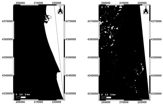
Figure 5.
Sea mask on the left: the black areas represent terrestrial and potentially flood-affected zones, while the white areas correspond to excluded marine regions. Cloud mask on the right: white areas represent cloud-covered regions excluded from the analysis, while black areas indicate cloud-free zones included in the study.
3.3. Index Calculation
In this study, six existing indices from the literature—NDWI, MNDWI-1, MNDWI-2, AWEIS, AWEINS, and NDFI—were applied to assess flooded areas. These indices were evaluated and compared to a novel index, the Flood Mud Index (FMI), which is introduced for the first time in this paper.
3.3.1. Normalized Difference Water Index (NDWI)
The Normalized Difference Water Index (NDWI), proposed by McFeeters [16], has been widely analyzed in the literature for its ability to effectively distinguish between water and soil. The formula for calculating the NDWI, previously presented as Formula 1, defines its range of variability between −1 and +1. In this range, the highest NDWI values are associated with water bodies [81].
3.3.2. Modified Normalized Difference Water Index-1 (MNDWI-1)
The Modified Normalized Difference Water Index (MNDWI), introduced by Xu in 2006 [23], replaces the near-infrared (NIR) band used in the NDWI with the shortwave infrared (SWIR) band. In this study, the variant that uses Band 6 (SWIR 1) is designed as MNDWI-1, with its formula provided below [82]:
Even in this case, the range of variability is between −1 and 1, with the highest values associated with flooded areas.
3.3.3. Modified Normalized Difference Water Index-2 (MNDWI-2)
MNDWI-2 is a variant of the MNDWI that utilizes Band 7 (SWIR 2) of the Landsat sensor. Its formula is expressed as follows [83]:
As previously mentioned, the range of variability is between −1 and 1, with the highest values associated with flooded areas.
3.3.4. Automated Water Extraction Index—No Shadows (AWEINS)
The Automated Water Extraction Index (AWEI) was initially developed and tested using imagery from the Landsat 5 satellite. The AWEINS was specifically designed to effectively exclude non-water pixels, including dark urban surfaces, in areas with an urban background [28].
The “NS” in the name is included to specify that the index is suited for situations where shadows are not a major problem.
3.3.5. Automated Water Extraction Index—Shadows (AWEIS)
The AWEIS index is primarily designed to enhance accuracy by addressing shadow pixels that AWEINS may not successfully exclude [28].
The subscript “S” in Equation (5) signifies that the equation is specifically designed to eliminate shadow pixels and enhance water extraction accuracy in regions with shadows and other dark surfaces.
3.3.6. NDFI
Developed as an advancement of the index proposed by Boschetti et al. [84], the Normalized Difference Flood Index (NDFI) is specifically designed for flood monitoring. Its formula is as follows [36]:
NDFI is designed to be sensitive to muddy waters as a result of sediment transportation in the flood.
3.3.7. New Index Proposal: Flood Mud Index (FMI)
The Flood Mud Index (FMI) is calculated using the red and blue bands, as expressed in the following formula:
This index was developed because other indices often fail to identify areas with high sediment content, such as muddy regions, as flooded. Figure 2 illustrates the situation in the hours immediately following the flooding: the inundated areas appear brownish due to the presence of sediment. For this reason, the red band was chosen instead of the SWIR band to improve the detection of these sediment-laden floodwaters.
3.4. Classification
Supervised classification relies on prior knowledge of sample classes within the image, known as training sites [85]. This approach involves analyzing pixel reflectance values to assign each pixel to the class it most closely resembles [86]. The success of supervised classification depends heavily on the careful selection of training sites, which must meet specific criteria to ensure accurate results. These criteria include being representative of all land cover classes in the image, containing a sufficient number of pixels for each class to enable reliable statistical estimation, and capturing the variability of spectral signatures among different classes [87,88]. For this work, supervised classification was employed to classify pixels into two distinct categories: Mud and No-Mud.
3.4.1. Maximum Likelihood Classification
In this study, the Maximum Likelihood Classification (MLC) method was chosen as one of the supervised classification techniques. MLC is grounded in Bayesian probability theory [89], estimating the statistical parameters (means and variances) of each class from the training data. These parameters are then used to calculate the probability of each pixel belonging to a specific class, assigning it to the class with the highest likelihood [90]. MLC is recognized in the literature as one of the most accurate classification methods, provided that well-chosen and representative training sites are available [91].
Although MLC is typically applied across multiple bands to take advantage of the full spectral range, it can also be applied to a single band [92].
3.4.2. Decision Tree
Decision Tree (DT) classification is a widely used supervised machine learning method that organizes data into a tree-like structure based on attribute-based decision rules. Its non-parametric nature and efficiency in handling complex classification tasks make it a popular choice for remote sensing applications [93]. The DT algorithm recursively splits the dataset into subsets using a series of binary decisions based on feature values, aiming to maximize class separability at each step [94].
A decision tree consists of three main components: nodes, branches, and leaves. Each internal node represents a decision based on a specific attribute, branches denote possible outcomes of that decision, and leaf nodes correspond to the final classification labels [95]. The tree-building process continues until a predefined stopping criterion is met, such as a minimum number of samples per leaf or a purity threshold.
3.4.3. Support Vector Machine
Support Vector Machine (SVM) is a non-parametric supervised learning algorithm widely used for classification tasks, particularly when the relationship between variables is complex or unknown. Based on statistical learning theory, SVM is designed to find an optimal hyperplane that maximizes the margin between different classes [96]. The core principle of SVM is to determine the hyperplane that best separates the data by maximizing the margin, defined as the distance between the hyperplane and the closest data points, known as support vectors. This maximization ensures a robust classification that generalizes well to unseen data [97]. When the data is not linearly separable, kernel functions such as radial basis function (RBF) or polynomial kernels allow SVM to capture complex decision boundaries.
SVM is particularly effective for high-dimensional datasets and has demonstrated strong performance in remote sensing applications, including land cover classification and flood mapping. However, its computational complexity can be a limitation, especially for large datasets, requiring optimization techniques to improve efficiency [98].
3.5. Accuracy Assessment
To evaluate the thematic accuracy of the classification results, test sites were utilized. These test sites, distinct from the training sites, were selected through visual analysis of the multispectral images and were designed to represent the two classes: Mud and No-Mud [99]. The primary tool for this evaluation was the confusion matrix, a widely used method in remote sensing studies. The confusion matrix establishes the correspondence between classification outcomes and ground truth data (i.e., the test sites) [100]. The thematic accuracy of the classification method was summarized using three key metrics [101]: Producer Accuracy, User Accuracy, and Overall Accuracy.
Producer Accuracy (PA)—Indicates the probability that a specific land cover class on the ground is correctly classified. For each class, it is calculated as the ratio of correctly classified pixels to the total reference pixels in that class:
where CAk is the correctly classified pixels of classk, while PBk is the total pixels belonging to the class considered.
User Accuracy (UA)—Represents the likelihood that a pixel classified into a specific category actually corresponds to that category on the ground. It is determined by dividing the number of correctly classified pixels in a class by the total pixels classified as belonging to that class.
where CAk is the number of correctly classified pixels of classk, and PCk is the number of the pixels that classify into classk.
Overall Accuracy (OA)—Reflects the overall proportion of correctly classified pixels across all categories, calculated by dividing the total number of correctly classified pixels by the total number of reference pixels.
where CAk, CAl, … CAz indicate the number of pixels correctly classified for each class (k,l…,z), while P is the total number of pixels used.
To ensure reliable accuracy assessment, it is crucial to select training and test samples in a balanced manner between the Mud and No-Mud classes. A well-distributed sampling strategy minimizes bias and enhances the representativeness of the classification process. In this study, 1500 pixels per class were used for training, corresponding to an approximate area of 1,350,000 m2. Similarly, 1000 pixels per class were designated for accuracy assessment, covering an approximate area of 900,000 m2.
Figure 6 illustrates the spatial distribution of the training and test sites, highlighting the areas used to train the classification model and evaluate its performance.
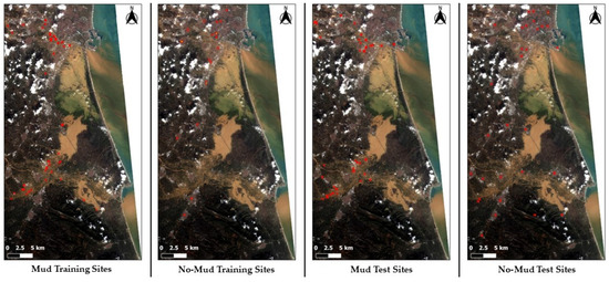
Figure 6.
Spatial distribution of training and test sites used for classification. The red points represent selected locations for Mud and No-Mud classes. The first two images illustrate the training sites, while the latter two depict the test sites.
4. Results and Discussion
Before delving into quantitative evaluations, a preliminary visual analysis of the spectral indices, shown in Figure 7, was conducted to assess their ability to delineate flooded areas.
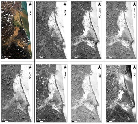
Figure 7.
An overview of the different indices applied in this study, including NDWI, MNDWI-1, MNDWI-2, AWEIS, AWEINS, NDFI, and the proposed FMI, alongside the RGB composite for reference. In the RGB composition, mud-covered areas appear brownish, while in the index maps, these areas are represented by brighter pixels.
The NDWI demonstrates high sensitivity to water bodies but struggles to effectively distinguish sediment-laden floodwaters from surrounding land, leading to potential misclassifications.
MNDWI-1 improves the delineation of water bodies but still faces challenges in detecting regions with high debris concentrations. MNDWI-2 provides a slightly sharper contrast for sediment-laden areas but is still not very effective overall.
While AWEIS appears less promising at first glance, AWEINS shows a slightly better ability to distinguish areas with significant sediment content.
The NDFI exhibits good sensitivity to flooded areas. However, regions with high sediment concentrations tend to blend with the surrounding land, limiting its capacity to accurately differentiate these areas. Additionally, it appears to overestimate flooded zones in some cases.
The FMI, proposed in this study, performs remarkably well in identifying muddy floodwaters. Areas with high sediment concentrations, which appear brownish in the RGB reference image, are effectively captured by the FMI. Compared to the other indices, the FMI demonstrates a stronger response to the spectral characteristics of sediment-laden floodwaters, minimizing misclassifications and providing a clearer delineation of these regions.
The classification results for the different indices are presented in Figure 8, Figure 9 and Figure 10, where each map highlights the areas identified as “Mud” (white) and “No-Mud” (black).
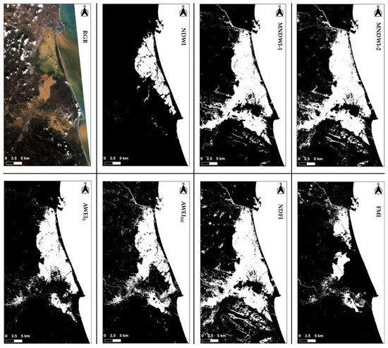
Figure 8.
Results of the MLC of the different indices. The maps illustrate the delineation of flooded areas for NDWI, MNDWI-1, MNDWI-2, AWEIS, AWEINS, NDFI, and FMI. The binary outputs highlight the regions classified as “Mud” (white) and “No-Mud” (black) for each index.
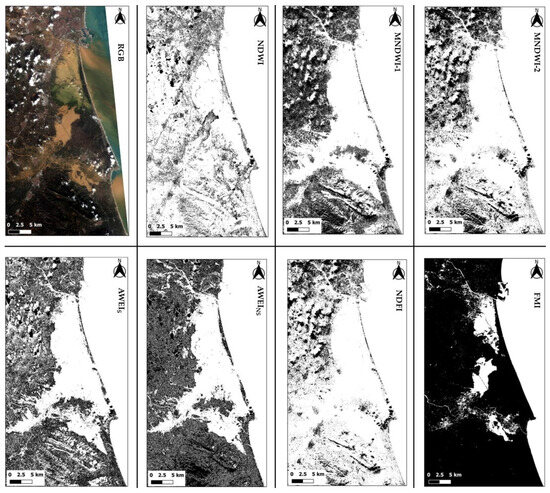
Figure 9.
Results of the DT classification of the different indices. The maps illustrate the delineation of flooded areas for NDWI, MNDWI-1, MNDWI-2, AWEIS, AWEINS, NDFI, and FMI. The binary outputs highlight the regions classified as “Mud” (white) and “No-Mud” (black) for each index.
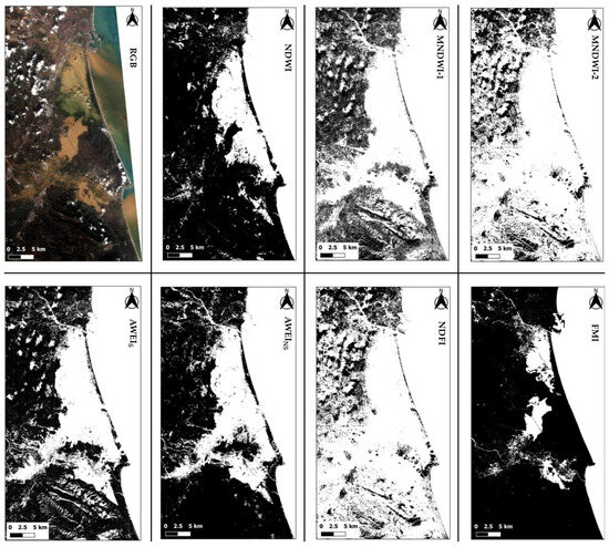
Figure 10.
Results of the SVM classification of the different indices. The maps illustrate the delineation of flooded areas for NDWI, MNDWI-1, MNDWI-2, AWEIS, AWEINS, NDFI, and FMI. The binary outputs highlight the regions classified as “Mud” (white) and “No-Mud” (black) for each index.
The classification results were processed after the application of sea and cloud masks. These masks were employed to exclude marine areas and cloud-covered regions from the analysis, ensuring that only relevant terrestrial and cloud-free areas are considered. This preprocessing step enhances the reliability of the classification, allowing for a clearer assessment of the indices’ performance in detecting mud-covered areas.
In Figure 8, it is clear that the NDWI fails to classify areas covered by mud, instead highlighting only regions with clear water. This limitation underscores the index’s inability to detect sediment-laden floodwaters, making its performance inadequate for this application.
The MNDWI-1 and MNDWI-2 indices perform significantly better in identifying areas flooded with mud. Notably, MNDWI-2 captures a larger extent of flooded regions, particularly in the northern part of the image. However, it also misclassifies shadowed areas in the southern region as flooded, highlighting a limitation in its accuracy.
The AWEIS index fails to identify many of the mud-covered areas in the northern part of the image. In contrast, the AWEINS index appears to be the most promising among the indices from the existing literature.
The NDFI significantly overestimates flooded areas compared to the other indices. However, it fails to capture some key flooded regions in the northern part of the image.
Finally, the FMI appears to accurately capture most of the areas flooded with mud.
Figure 9 presents the classification results obtained using the Decision Tree (DT) algorithm. NDWI exhibits severe overestimation, classifying almost the entire scene as flooded. This misclassification is particularly evident in mountainous and vegetated areas, which are incorrectly identified as mud-covered regions. The absence of clear delineation between actual flood zones and surrounding terrain highlights NDWI’s inability, in this case, to distinguish between water-saturated land and true floodwater.
MNDWI-2 exhibits some misclassification in the southern portion of the image, where shadowed areas are wrongly classified as flooded. This issue is less pronounced in MNDWI-1, though it still appears to underestimate some of the heavily sediment-laden regions.
Also, AWEIS shows significant overestimation, failing to classify large portions of the non-mud-covered areas. AWEINS performs better than AWEIS, better capturing flood areas. However, it still overestimates the extension of flooding. Indeed, it presents some “salt and pepper effect” in non-mud-covered areas.
NDFI strongly overestimates the extent of flooding, showing a tendency to over-detect water.
FMI provides the most accurate flood delineation, successfully identifying key muddy flood zones while avoiding excessive overestimation. Unlike the other indices, FMI is able to capture the extent of mud-covered areas with high precision, never showing noise effects.
Figure 10 presents the classification results obtained using the SVM method.
NDWI exhibits severe underestimation, as most of the scene remains classified as non-flooded (black). This confirms its inability to capture mud-covered areas, making it unreliable for this specific task.
MNDWI-1 and MNDWI-2 improve flood detection compared to NDWI. MNDWI-2, in particular, captures a more extensive flooded region, especially in the northern and central parts of the study area. However, it continues to misclassify shadowed areas as flooded regions, particularly in the southern portion of the image. MNDWI-1, while slightly more conservative, still struggles to delineate sediment-rich waters accurately.
AWEIS produces a scattered classification, failing to detect some flooded zones and overestimating mud presence in other areas. The index sometimes seems to struggle with differentiating muddy water from dry land.
AWEINS performs better than AWEIS, better identifying the flooded terrain. However, it still misses critical flooded regions near river deltas and highly sediment-laden zones. This suggests that AWEINS is sensitive to water presence but struggles with highly turbid conditions.
NDFI significantly overestimates flooded areas, classifying large portions of the terrain as inundated.
FMI, once again, outperforms all other indices, providing the most accurate delineation of sediment-rich flooded zones. Compared to the other indices, FMI correctly highlights the brownish flood-affected areas observed in the RGB composite, demonstrating superior adaptability to muddy conditions.
Compared to other classification methods, MLC produces more defined flood boundaries, reducing ambiguity in flood extent interpretation. Therefore, two zoomed-in views of the MLC classification are presented, highlighting key areas of interest: one focusing on the northern section of the study area and another on the southern region.
Figure 11 presents a detailed view of a specific flooded area in the northern part of the clip (5 km × 5 km), close to the city of Valencia, classified using MLC.
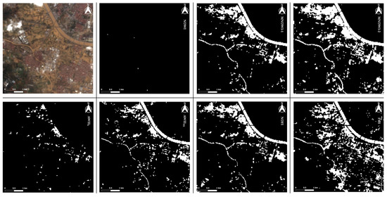
Figure 11.
Detail (north) of the classification of the indices. The maps illustrate the delineation of flooded areas for NDWI, MNDWI-1, MNDWI-2, AWEIS, AWEINS, NDFI, and FMI. Mud in white, No-Mud in black.
From Figure 11, it is even clearer that NDWI fails to detect most of the flooded areas, capturing only small water bodies while completely missing regions affected by sediment-heavy floodwaters.
MNDWI-1 and MNDWI-2 show a good delineation of flooded zones, with MNDWI-2 providing slightly better coverage. However, MNDWI-2 overestimates the mud coverage in some areas.
The AWEIS index struggles with detection in this detailed area, capturing only limited flooded regions. Conversely, AWEINS performs noticeably better, identifying larger areas of flooding, though some misclassification remains apparent.
The NDFI captures a significant portion of the flooded area but still misses some mud-covered spots.
The FMI, proposed in this study, offers the most accurate representation of the flooded areas, effectively delineating regions impacted by sediment-laden waters. It clearly captures areas missed or misclassified by other indices. This is particularly evident in the southern part of the detail, where the FMI is the only index capable of accurately identifying that region as being covered by mud.
Figure 12 shows further details of another flooded area in the south (9 km × 9 km).
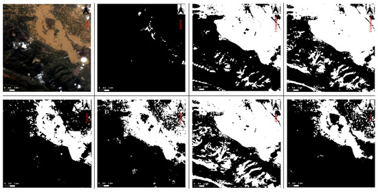
Figure 12.
Detail (south) of the classification of the indices. The maps illustrate the delineation of flooded areas for NDWI, MNDWI-1, MNDWI-2, AWEIS, AWEINS, NDFI, and FMI. Mud in white, No-Mud in black.
The NDWI, once again, fails entirely to identify the majority of the flooded region, as it is unable to capture the spectral characteristics of sediment-laden waters, leaving most areas undetected.
Both MNDWI-1 and MNDWI-2 tend to overestimate flooded areas. In particular, MNDWI-2 misclassifies shadowed regions as flooded more than MNDWI-1.
AWEIS shows inconsistencies, overestimating flooded areas in some regions while underestimating them in others. In contrast, AWEINS provides a clearer representation of the flooded regions, but some noise and misclassifications remain visible.
The NDFI heavily overestimates the extent of flooding, misclassifying shadowed or vegetated areas as flooded.
The FMI once again demonstrates superior accuracy, effectively capturing the shape of the mud-covered areas. It provides a precise delineation of the muddy floodwaters with minimal misclassification, making it the most effective index for this scenario.
The accuracy assessment results for each index, including User Accuracy (UA), Producer Accuracy (PA), and Overall Accuracy (OA), are summarized in Table 2, Table 3 and Table 4.
Table 2.
Thematic accuracy values for MLC of Landsat 8 OLI-derived products.
Table 3.
Thematic accuracy values for DT classification of Landsat 8 OLI-derived products.
Table 4.
Thematic accuracy values for SVM classification of Landsat 8 OLI-derived products.
While the NDWI achieves perfect UA (100%) for the “Mud” class, it fails almost entirely in detecting actual flooded areas with sediment, as shown by its very low PA (0.43%). This indicates that while the few areas classified as “Mud” are correct, the index misses almost all other flooded regions. This is reflected in its low OA (50.21%), making it unsuitable for identifying muddy floodwaters.
MNDWI-1 achieves an OA of 75.50%, while MNDWI-2 performs slightly better with 78.57%. MNDWI-2 shows higher PA for the “Mud” class (73.71% compared to 66.57% of MNDWI-1), which indicates its ability to capture more flooded areas. However, both indices still exhibit misclassifications, limiting their effectiveness.
The AWEINS index demonstrates strong performance, with a high OA of 82.29%. However, it presents low PA for the “Mud” class (66.00%) in contrast to the high PA for the “No-Mud” class (98.57%). Still, it is one of the more reliable indices from the existing literature. On the other hand, AWEIS shows lower accuracy, with an OA of 77.43%. It struggles with PA for the “Mud” class (57.43%), suggesting it underestimates these areas.
The NDFI exhibits moderate performance, with an OA of 74.50%. While it achieves a decent balance in User and Producer Accuracy for both classes, it tends to overestimate flooded areas; it is, in fact, the only one to have a UA lower than 80% for the “Mud” class.
The FMI, proposed in this study, stands out as the most effective index, achieving the highest OA of 97.64%. It provides a nearly perfect balance between User and Producer Accuracy for both classes, with values exceeding 97% across all metrics. This indicates that the FMI not only identifies sediment-laden floodwaters with exceptional precision but also avoids significant misclassification. Its superior performance highlights its robustness and suitability for mapping muddy floodwaters compared to other indices.
As shown in Table 3, a noticeable trend reversal is observed in User Accuracy (UA) and Producer Accuracy (PA) values compared to those obtained with MLC (Table 2). This shift aligns with the classification patterns visible in Figure 8 and Figure 9, corresponding to MLC and DT, respectively.
In particular, a higher PA value for a given class suggests an overestimation of that class. While MLC tended to overestimate the No-Mud class, DT-based classification consistently overestimates the Mud class across all indices. This trend holds for all indices except FMI, which maintains well-balanced UA, PA, and OA values.
FMI remains the only index achieving UA, PA, and OA values above 97%, reinforcing its robustness in detecting sediment-laden flooded areas. The only other index approaching a comparable balance between PA and UA is AWEINS, but it still falls short of FMI’s overall performance and classification reliability.
Regarding the other indices, NDWI remains the least effective, performing poorly in accurately classifying flooded areas. MNDWI-2 exhibits a strong overestimation of Mud (PA = 91.00%), misclassifying some No-Mud areas as Mud, as seen in Figure 9. Similarly, NDFI struggles with commission errors, showing one of the largest discrepancies between UA (65.89%) and PA (89.14%) for the Mud class.
Table 4 presents the accuracy metrics obtained using the Support Vector Machine (SVM) classifier. FMI once again stands out as the most consistent and well-balanced index, achieving UA, PA, and OA values all above 97%, confirming its robustness across different classification methods.
AWEINS performs relatively well, showing values close to its MLC-based counterpart (Table 2). However, it still fails to classify certain muddy areas, leading to slightly lower PA for Mud (75.14%) compared to FMI. Notably, among the three classification methods applied (MLC, DT, and SVM), AWEINS achieves its highest OA (85%) using SVM. AWEIS shows similar behavior to AWEINS but misclassifies shadowed regions (both cloud and terrain shadows) as flooded areas, reducing its overall reliability.
As for NDWI, its performance remains closer to its MLC-based counterpart, again underestimating the presence of Mud, as indicated by its low PA for Mud (30.00%), meaning many actual flooded areas were not identified.
The other indices exhibit a strong tendency to overestimate flooded areas, with MNDWI-2 and NDFI being the most affected by this issue. In particular, MNDWI-2 records a PA for Mud of 91.14%, confirming a strong overclassification of non-flooded areas as flooded, in agreement with Figure 10.
The results obtained in this study are consistent with findings from previous research that applied the same spectral indices for flood mapping. The NDWI is widely recognized as an effective indicator for detecting clear water bodies, but its performance declines significantly in the presence of high turbidity levels [102,103]. In contrast, the MNDWI, introduced by Xu, has demonstrated improved sensitivity to turbid waters, making it more suitable for identifying flooded areas [39,102,103]. Furthermore, the overestimation tendency of MNDWI, particularly in the presence of shadowed areas, has been widely reported in the literature [27]. This phenomenon is especially evident in MNDWI-2, which, as observed in this study, frequently misclassifies shadowed regions as flooded areas. The effectiveness of these indices is highly dependent on the specific characteristics of the study area. For instance, in Khalifeh Soltanian et al. (2019) [24], an analysis of the 2018 and 2019 floods in the Aghqala region of Iran demonstrated that NDWI produced more reliable results compared to MNDWI, which was excessively sensitive and misclassified agricultural wetlands as water bodies. This highlights the importance of considering regional land cover characteristics when selecting the most appropriate index for flood detection.
Among the indices from the existing literature, AWEINS demonstrated the best performance in this study. This aligns with findings from Farhadi et al. (2024) [104], where AWEINS performed well across all subsets, consistently achieving UA values above 85%. In contrast, AWEIS results in this study were affected by shadowed areas, which were consistently misclassified as mud-covered regions. The superior accuracy of AWEIa over AWEIS has also been noted by Goffi et al. (2020) [30]. Moreover, Goffi et al. [30] pointed out that the NDFI response is similar to NDWI, making it effective for detecting clear water but less suitable for highly turbid floodwaters.
The proposed FMI has proven to be highly effective in identifying muddy floodwaters with high turbidity. However, if this study had focused on a low-turbidity flood event (i.e., clear water flooding), FMI might not have been among the best-performing indices. The key limitation of FMI is that it is specifically optimized for mud detection. Therefore, a preliminary visual analysis of the study area is essential to ensure the suitability of FMI for a given flood scenario.
A potential future improvement could involve combining the results of NDWI and FMI, as these indices appear to be the most decorrelated among all tested. NDWI excels at detecting clear water bodies, whereas FMI performs well in identifying muddy floodwaters, making their complementary use a promising approach for more robust flood delineation.
Finally, the selection of training and test sites was based on visual interpretation, which, while ensuring careful identification of flood-affected areas, introduces a degree of subjectivity. Future studies could incorporate automated or semi-automated sampling techniques to improve reproducibility and minimize potential selection biases or other methods such as LSU.
5. Conclusions
This study aimed to address the limitations of existing spectral indices in detecting mud-covered areas, a challenge that is particularly evident in the aftermath of extreme flooding events. Through the comparative analysis of six widely used indices (NDWI, MNDWI-1, MNDWI-2, AWEINS, AWEIS, and NDFI) and the newly proposed Flood Mud Index (FMI), significant insights were gained into their performance in mapping muddy floodwaters.
The results indicate that traditional indices, such as NDWI, are ineffective for this purpose, as they primarily identify clear water bodies and fail to detect areas covered by sediment-laden floodwaters. MNDWI-1, MNDWI-2, and NDFI showed good performance but suffered from overestimation, particularly in shadowed regions. Similarly, AWEINS emerged as one of the more promising indices from the existing literature, achieving good accuracy but still misclassifying certain areas.
The FMI, introduced in this study, outperformed all other indices, achieving an Overall Accuracy of 97.64% and consistently high User and Producer Accuracy across both the “Mud” and “No-Mud” classes. The FMI’s ability to precisely capture sediment-laden flooded areas was particularly evident in both regional and detailed analyses, where it successfully identified areas missed or misclassified by other indices. This performance underscores the FMI’s potential as a robust tool for flood mapping in scenarios involving high sediment content.
From a practical perspective, the FMI is particularly advantageous as it relies only on the red and blue bands, making it compatible with a wide range of satellite and drone-based sensors. This adaptability is crucial for emergency response efforts, where timely and accurate information about flood extent is necessary. The FMI’s effectiveness in detecting muddy floodwaters can help improve disaster management strategies, providing better situational awareness for affected areas.
Future research could focus on testing the FMI in other flood-prone regions to further validate its performance and explore its integration with other remote sensing data, such as synthetic aperture radar (SAR), for even more comprehensive flood assessments.
Satellite-based methods enable large-scale flood monitoring, making them particularly valuable in widespread disaster scenarios where UAV deployment may be impractical due to logistical or weather-related constraints. However, expanding the use of the FMI to drone-based platforms could provide valuable insights for local-scale applications, particularly in scenarios where satellite imagery is unavailable or obscured by cloud cover. While this study demonstrates the effectiveness of FMI in mapping muddy floodwaters using satellite data, future research could integrate UAV imagery and ground validation to further refine accuracy and improve applicability across different flood conditions.
Furthermore, some valuable methods, such as LSU, were not applied in this paper. Future research could explore its applicability alongside spectral indices to assess its potential advantages and limitations in detecting sediment-laden floodwaters.
Funding
This research received no external funding.
Data Availability Statement
The study’s data is available upon request from the corresponding author for academic research and non-commercial purposes only. Restrictions apply to derivative images and models trained using the data, and proper referencing is required.
Conflicts of Interest
The author declares no conflict of interest.
References
- Getahun, Y.S.; Gebre, S.L. Flood hazard assessment and mapping of flood inundation area of the Awash River Basin in Ethiopia using GIS and HEC-GeoRAS/HEC-RAS model. J. Civ. Environ. Eng. 2015, 5, 1–12. [Google Scholar] [CrossRef]
- Mudashiru, R.B.; Sabtu, N.; Abustan, I.; Balogun, W. Flood hazard mapping methods: A review. J. Hydrol. 2021, 603, 126846. [Google Scholar] [CrossRef]
- Alcaras, E.; Mercogliano, P.; Morale, D.; Parente, C. GIS analysis for defining sea level rise effects on Sicily coasts for the end of the 21st century. In Proceedings of the 2023 IEEE International Workshop on Metrology for the Sea; Learning to Measure Sea Health Parameters (MetroSea), La Valletta, Malta, 4–6 October 2023; IEEE: New York, NY, USA, 2023; pp. 62–66. [Google Scholar] [CrossRef]
- Jonkman, S.N.; Vrijling, J.K. Loss of life due to floods. J. Flood Risk Manag. 2008, 1, 43–56. [Google Scholar] [CrossRef]
- United Nations. International Stratety for Disaster Reduction. Secretariat, & International Strategy for Disaster Reduction. Global Assessment Report on Disaster Risk Reduction. 2015. Available online: https://www.undrr.org/quick/11404 (accessed on 29 November 2024).
- Tabari, H. Climate change impact on flood and extreme precipitation increases with water availability. Sci. Rep. 2020, 10, 13768. [Google Scholar] [CrossRef] [PubMed]
- European Union: Directive 2007/60/EC of the European Council and European Parliament of 23 October 2007 on the Assessment and Management of Flood Risks, Official Journal of the European Union, 27–34. Available online: http://data.europa.eu/eli/dir/2007/60/oj (accessed on 29 November 2024).
- Díaz-Delgado, R.; Aragonés, D.; Afán, I.; Bustamante, J. Long-term monitoring of the flooding regime and hydroperiod of Doñana marshes with Landsat time series (1974–2014). Remote Sens. 2016, 8, 775. [Google Scholar] [CrossRef]
- McCormack, T.; Campanyà, J.; Naughton, O. A methodology for mapping annual flood extent using multi-temporal Sentinel-1 imagery. Remote Sens. Environ. 2022, 282, 113273. [Google Scholar] [CrossRef]
- Schumann, G.J.; Brakenridge, G.R.; Kettner, A.J.; Kashif, R.; Niebuhr, E. Assisting flood disaster response with earth observation data and products: A critical assessment. Remote Sens. 2018, 10, 1230. [Google Scholar] [CrossRef]
- Jain, S.K.; Singh, R.D.; Jain, M.K.; Lohani, A.K. Delineation of flood-prone areas using remote sensing techniques. Water Resour. Manag. 2005, 19, 333–347. [Google Scholar] [CrossRef]
- Jongman, B.; Wagemaker, J.; Revilla Romero, B.; Coughlan de Perez, E. Early flood detection for rapid humanitarian response: Harnessing near real-time satellite and Twitter signals. ISPRS Int. J. Geo-Inf. 2015, 4, 2246–2266. [Google Scholar] [CrossRef]
- Rahman, M.S.; Di, L. The state of the art of spaceborne remote sensing in flood management. Nat. Hazards 2017, 85, 1223–1248. [Google Scholar] [CrossRef]
- Wang, X.; Xie, H. A review on applications of remote sensing and geographic information systems (GIS) in water resources and flood risk management. Water 2018, 10, 608. [Google Scholar] [CrossRef]
- Notti, D.; Giordan, D.; Caló, F.; Pepe, A.; Zucca, F.; Galve, J.P. Potential and limitations of open satellite data for flood mapping. Remote Sens. 2018, 10, 1673. [Google Scholar] [CrossRef]
- McFeeters, S.K. The use of the Normalized Difference Water Index (NDWI) in the delineation of open water features. Int. J. Remote Sens. 1996, 17, 1425–1432. [Google Scholar] [CrossRef]
- Ji, L.; Geng, X.; Sun, K.; Zhao, Y.; Gong, P. Target detection method for water mapping using Landsat 8 OLI/TIRS imagery. Water 2015, 7, 794–817. [Google Scholar] [CrossRef]
- Nozarpour, N.; Gharechelou, S.; Rafiee, F. Flood zoning using Sentinel 1–2 and Landsat-8 data in Khuzestan province. In Proceedings of the 12th International Congress on Civil Engineering, Mashhad, Iran, 12–14 July 2021; Ferdowsi University of Mashhad: Mashhad, Iran, 2021. [Google Scholar]
- Memon, A.A.; Muhammad, S.; Rahman, S.; Haq, M. Flood monitoring and damage assessment using water indices: A case study of Pakistan flood-2012. Egypt. J. Remote Sens. Space Sci. 2015, 18, 99–106. [Google Scholar] [CrossRef]
- Dash, P.; Sar, J. Identification and validation of potential flood hazard area using GIS-based multi-criteria analysis and satellite data-derived water index. J. Flood Risk Manag. 2020, 13, e12620. [Google Scholar] [CrossRef]
- Gebrehiwot, A.; Hashemi-Beni, L. Automated indunation mapping: Comparison of methods. In Proceedings of the IGARSS 2020–2020 IEEE International Geoscience and Remote Sensing Symposium, Waikoloa, HI, USA, 26 September–2 September 2020; IEEE: New York, NY, USA, 2020; pp. 3265–3268. [Google Scholar] [CrossRef]
- Singh, S.; Kansal, M.L. Chamoli flash-flood mapping and evaluation with a supervised classifier and NDWI thresholding using Sentinel-2 optical data in Google earth engine. Earth Sci. Inform. 2022, 15, 1073–1086. [Google Scholar] [CrossRef]
- Xu, H. Modification of normalised difference water index (NDWI) to enhance open water features in remotely sensed imagery. Int. J. Remote Sens. 2006, 27, 3025–3033. [Google Scholar] [CrossRef]
- Khalifeh Soltanian, F.; Abbasi, M.; Riyahi Bakhtyari, H.R. Flood monitoring using ndwi and mndwi spectral indices: A case study of aghqala flood-2019, Golestan Province, Iran. Int. Arch. Photogramm. Remote Sens. Spat. Inf. Sci. 2019, 42, 605–607. [Google Scholar] [CrossRef]
- Mehmood, H.; Conway, C.; Perera, D. Mapping of flood areas using landsat with google earth engine cloud platform. Atmosphere 2021, 12, 866. [Google Scholar] [CrossRef]
- Afzal, M.A.; Ali, S.; Nazeer, A.; Khan, M.I.; Waqas, M.M.; Aslam, R.A.; Cheema, M.J.M.; Nadeem, M.; Saddique, N.; Muzammil, M.; et al. Flood inundation modeling by integrating HEC–RAS and satellite imagery: A case study of the Indus River Basin. Water 2022, 14, 2984. [Google Scholar] [CrossRef]
- Albertini, C.; Gioia, A.; Iacobellis, V.; Manfreda, S. Detection of surface water and floods with multispectral satellites. Remote Sens. 2022, 14, 6005. [Google Scholar] [CrossRef]
- Feyisa, G.L.; Meilby, H.; Fensholt, R.; Proud, S.R. Automated Water Extraction Index: A new technique for surface water mapping using Landsat imagery. Remote Sens. Environ. 2014, 140, 23–35. [Google Scholar] [CrossRef]
- Deruyter, G.; Glas, H.; Piette, T. Semi-automatic flood detection using historic satellite imagery. In Proceedings of the International Multidisciplinary Scientific GeoConference: SGEM, Albena, Bulgaria, 2–8 July 2018; Volume 18, pp. 551–558. [Google Scholar] [CrossRef]
- Goffi, A.; Stroppiana, D.; Brivio, P.A.; Bordogna, G.; Boschetti, M. Towards an automated approach to map flooded areas from Sentinel-2 MSI data and soft integration of water spectral features. Int. J. Appl. Earth Obs. Geoinf. 2020, 84, 101951. [Google Scholar] [CrossRef]
- Duplančić Leder, T.; Leder, N.; Baučić, M. Application of satellite imagery and water indices to the hydrography of the Cetina River Basin (Middle Adriatic). Trans. Marit. Sci. 2020, 9, 374–384. [Google Scholar] [CrossRef]
- Al-Ali, Z.; Abulibdeh, A.; Al-Awadhi, T.; Mohan, M.; Al Nasiri, N.; Al-Barwani, M.; Al Nabbi, S.; Abdullah, M. Examining the potential and effectiveness of water indices using multispectral sentinel-2 data to detect soil moisture as an indicator of mudflow occurrence in arid regions. Int. J. Appl. Earth Obs. Geoinf. 2024, 130, 103887. [Google Scholar] [CrossRef]
- Haibo, Y.; Zongmin, W.; Hongling, Z.; Yu, G. Water body extraction methods study based on RS and GIS. Procedia Environ. Sci. 2011, 10, 2619–2624. [Google Scholar] [CrossRef]
- Alcaras, E.; Amoroso, P.P.; Figliomeni, F.G.; Parente, C.; Prezioso, G. Accuracy Evaluation of Coastline Extraction Methods in Remote Sensing: A Smart Procedure for Sentinel-2 Images. Int. Arch. Photogramm. Remote Sens. Spat. Inf. Sci. 2022, 48, 13–19. [Google Scholar] [CrossRef]
- Zollini, S.; Dominici, D.; Alicandro, M.; Cuevas-González, M.; Angelats, E.; Ribas, F.; Simarro, G. New Methodology for Shoreline Extraction Using Optical and Radar (SAR) Satellite Imagery. J. Mar. Sci. Eng. 2023, 11, 627. [Google Scholar] [CrossRef]
- Wan, K.M.; Billa, L. Post-flood land use damage estimation using improved Normalized Difference Flood Index (NDFI3) on Landsat 8 datasets: December 2014 floods, Kelantan, Malaysia. Arab. J. Geosci. 2018, 11, 434. [Google Scholar] [CrossRef]
- Byun, Y.; Han, D. Relative radiometric normalization of bitemporal very high-resolution satellite images for flood change detection. J. Appl. Remote Sens. 2018, 12, 026021. [Google Scholar] [CrossRef]
- Peng, B.; Liu, X.; Meng, Z.; Huang, Q. Urban flood mapping with residual patch similarity learning. In Proceedings of the 3rd ACM SIGSPATIAL International Workshop on AI for Geographic Knowledge Discovery, Chicago, IL, USA, 5 November 2019; pp. 40–47. [Google Scholar] [CrossRef]
- Sivanpillai, R.; Jacobs, K.M.; Mattilio, C.M.; Piskorski, E.V. Rapid flood inundation mapping by differencing water indices from pre-and post-flood Landsat images. Front. Earth Sci. 2021, 15, 1–11. [Google Scholar] [CrossRef]
- Zhu, J.; Jin, Y.; Zhu, W.; Lee, D.K. High spatiotemporal-resolution mapping for a seasonal erosion flooding inundation using time-series Landsat and MODIS images. Sci. Rep. 2024, 14, 4203. [Google Scholar] [CrossRef]
- Baig, M.H.A.; Zhang, L.; Wang, S.; Jiang, G.; Lu, S.; Tong, Q. Comparison of MNDWI and DFI for water mapping in flooding season. In Proceedings of the 2013 IEEE international geoscience and remote sensing symposium-IGARSS, Melbourne, Australia, 21–26 July 2013; IEEE: New York, NY, USA, 2013; pp. 2876–2879. [Google Scholar]
- Ghalehteimouri, K.J.; Ros, F.C.; Rambat, S.; Nasr, T. Spatial and temporal water pattern change detection through the normalized difference water index (NDWI) for initial flood assessment: A case study of Kuala Lumpur 1990 and 2021. J. Adv. Res. Fluid Mech. Therm. Sci. 2024, 114, 178–187. [Google Scholar] [CrossRef]
- Keshava, N.; Mustard, J.F. Spectral unmixing. IEEE Signal Process. Mag. 2002, 19, 44–57. [Google Scholar] [CrossRef]
- Wang, Q.; Ding, X.; Tong, X.; Atkinson, P.M. Spatio-temporal spectral unmixing of time-series images. Remote Sens. Environ. 2021, 259, 112407. [Google Scholar] [CrossRef]
- Bangira, T.; Alfieri, S.M.; Menenti, M.; Van Niekerk, A.; Vekerdy, Z. A spectral unmixing method with ensemble estimation of endmembers: Application to flood mapping in the Caprivi floodplain. Remote Sens. 2017, 9, 1013. [Google Scholar] [CrossRef]
- Pour, A.B.; Ranjbar, H.; Sekandari, M.; El-Wahed, M.A.; Hossain, M.S.; Hashim, M.; Yousefi, M.; Zoheir, B.; Wambo, J.D.T.; Muslim, A.M. Remote sensing for mineral exploration. In Geospatial Analysis Applied to Mineral Exploration; Elsevier: Amsterdam, The Netherlands, 2023; pp. 17–149. [Google Scholar] [CrossRef]
- Guerra, R.; Santos, L.; López, S.; Sarmiento, R. A new fast algorithm for linearly unmixing hyperspectral images. IEEE Trans. Geosci. Remote Sens. 2015, 53, 6752–6765. [Google Scholar] [CrossRef]
- Borsoi, R.A.; Imbiriba, T.; Bermudez, J.C.M.; Richard, C.; Chanussot, J.; Drumetz, L.; Tourneret, J.-Y.; Zare, A.; Jutten, C. Spectral variability in hyperspectral data unmixing: A comprehensive review. IEEE Geosci. Remote Sens. Mag. 2021, 9, 223–270. [Google Scholar] [CrossRef]
- Ghosh, P.; Roy, S.K.; Koirala, B.; Rasti, B.; Scheunders, P. Hyperspectral unmixing using transformer network. IEEE Trans. Geosci. Remote Sens. 2022, 60, 1–16. [Google Scholar] [CrossRef]
- Somers, B.; Asner, G.P.; Tits, L.; Coppin, P. Endmember variability in spectral mixture analysis: A review. Remote Sens. Environ. 2011, 115, 1603–1616. [Google Scholar] [CrossRef]
- Pérez-Landa, G.; Ciais, P.; Sanz, M.J.; Gioli, B.; Miglietta, F.; Palau, J.L.; Gangoiti, G.; Millán, M.M. Mesoscale circulations over complex terrain in the Valencia coastal region, Spain–Part 1: Simulation of diurnal circulation regimes. Atmos. Chem. Phys. 2007, 7, 1835–1849. [Google Scholar] [CrossRef]
- Masachs-Alavedra, V. El Regimen de los ríos Peninsulares; CSIC: Barcelona, Spacin, 1948; 511p. [Google Scholar]
- Ruiz-Pérez, J.M.; Carmona, P. Turia river delta and coastal barrier-lagoon of Valencia (Mediterranean coast of Spain): Geomorphological processes and global climate fluctuations since Iberian-Roman times. Quat. Sci. Rev. 2019, 219, 84–101. [Google Scholar] [CrossRef]
- Carmona, P.; Ruiz, J.M. Historical morphogenesis of the Turia River coastal flood plain in the Mediterranean littoral of Spain. Catena 2011, 86, 139–149. [Google Scholar] [CrossRef]
- Ruiz, J.M.; Carmona, P.; Pérez Cueva, A. Flood frequency and seasonality of the Jucar and Turia Mediterranean rivers (Spain) during the “Little Ice Age”. Méditerranée. Rev. Géographique Des Pays Méditerranéens/J. Mediterr. Geogr. 2014, 122, 121–130. [Google Scholar] [CrossRef]
- FAO. Historical Irrigation System at l’Horta de València, Spain; Food and Agriculture Organization of the United Nations: Rome, Italy, 2019; Available online: https://openknowledge.fao.org/server/api/core/bitstreams/3c2710e7-5c70-4c0b-9777-b761cea4f000/content (accessed on 1 December 2024).
- Garcia, J.M. Environmental management of peri-urban natural resources: L’Horta de Valencia case study. In En: WIT Transactions on Ecology and the Environment; WIT Press Southampton: Ashurst, UK, 2015; Volume 192, pp. 99–110. [Google Scholar]
- Melo, C. L’Horta De València: Past and present dynamics in landscape change and planning. Int. J. Sustain. Dev. Plan. 2020, 15, 28–44. [Google Scholar] [CrossRef]
- Soria, J.M. Past, present and future of la Albufera of Valencia Natural Park. Limnetica 2006, 25, 135–142. [Google Scholar] [CrossRef]
- Canet, R.; Chaves, C.; Pomares, F.; Albiach, R. Agricultural use of sediments from the Albufera Lake (eastern Spain). Agric. Ecosyst. Environ. 2003, 95, 29–36. [Google Scholar] [CrossRef]
- Sòria-Perpinyà, X.; Urrego, P.; Pereira-Sandoval, M.; Ruiz-Verdú, A.; Peña, R.; Soria, J.M.; Moreno, J. Monitoring the ecological state of a hypertrophic lake (Albufera of València, Spain) using multitemporal Sentinel-2 images. Limnetica 2019, 38, 457–469. [Google Scholar] [CrossRef]
- Martín, M.; Hernández-Crespo, C.; Andrés-Doménech, I.; Benedito-Durá, V. Fifty years of eutrophication in the Albufera lake (Valencia, Spain): Causes, evolution and remediation strategies. Ecol. Eng. 2020, 155, 105932. [Google Scholar] [CrossRef]
- Segrelles, C.E.E.; Martín, M.Á.P.; Martínez, G.G. Climate change impacts on a Mediterranean coastal wetland due to sea level rise (L’Albufera de Valencia, Spain). Copernic. Meet. 2021, EGU21, 1599. [Google Scholar] [CrossRef]
- Soria, J.M.; Vicente, E.; Miracle, M.R. The influence of flash floods on the limnology of the Albufera of Valencia lagoon (Spain). Int. Ver. Theor. Angew. Limnol. Verhandlungen 2000, 27, 2232–2235. [Google Scholar] [CrossRef]
- Cavallo, C.; Papa, M.N.; Gargiulo, M.; Palau-Salvador, G.; Vezza, P.; Ruello, G. Continuous monitoring of the flooding dynamics in the Albufera Wetland (Spain) by Landsat-8 and Sentinel-2 datasets. Remote Sens. 2021, 13, 3525. [Google Scholar] [CrossRef]
- Perilla, O.L.U.; Gómez, A.G.; Gómez, A.G.; Díaz, C.Á.; Cortezón, J.A.R. Methodology to assess sustainable management of water resources in coastal lagoons with agricultural uses: An application to the Albufera lagoon of Valencia (Eastern Spain). Ecol. Indic. 2012, 13, 129–143. [Google Scholar] [CrossRef]
- Cerdà, A.; Imeson, A.C.; Calvo, A. Fire and aspect induced differences on the erodibility and hydrology of soils at La Costera, Valencia, southeast Spain. Catena 1995, 24, 289–304. [Google Scholar] [CrossRef]
- Soria, J.; Vera-Herrera, L.; Calvo, S.; Romo, S.; Vicente, E.; Sahuquillo, M.; Sòria-Perpinyà, X. Residence time analysis in the albufera of Valencia, a Mediterranean Coastal Lagoon, Spain. Hydrology 2021, 8, 37. [Google Scholar] [CrossRef]
- Belmonte, A.M.C.; Beltrán, F.S. Flood events in Mediterranean ephemeral streams (ramblas) in Valencia region, Spain. Catena 2001, 45, 229–249. [Google Scholar] [CrossRef]
- Portugués-Mollá, I.; Bonache-Felici, X.; Mateu-Bellés, J.F.; Marco-Segura, J.B. A GIS-Based Model for the analysis of an urban flash flood and its hydro-geomorphic response. The Valencia event of 1957. J. Hydrol. 2016, 541, 582–596. [Google Scholar] [CrossRef]
- Sanjaume, E.; Pardo-Pascual, J.E. Erosion by human impact on the Valencian coastline (E of Spain). J. Coast. Res. 2005, SI 49, 76–82. [Google Scholar]
- U.S. Geological Survey. Landsat 8 (L8) Data Users Handbook—Version 5.0. November 2019. Available online: https://d9-wret.s3.us-west-2.amazonaws.com/assets/palladium/production/s3fs-public/atoms/files/LSDS-1574_L8_Data_Users_Handbook-v5.0.pdf (accessed on 1 December 2024).
- NASA—USGS. Landsat 9. 2022. Available online: https://landsat.gsfc.nasa.gov/satellites/landsat-9/ (accessed on 1 December 2024).
- Campbell, J.B.; Wynne, R.H. Introduction to Remote Sensing; Guilford Press: New York, NY, USA, 2011. [Google Scholar]
- Chavez, P.S., Jr. An improved dark-object subtraction technique for atmospheric scattering correction of multispectral data. Remote Sens. Environ. 1988, 24, 459–479. [Google Scholar] [CrossRef]
- Viñals, M.J.; Vizcauno, A.; Benavent, J.M.; Romo, S. Restoring a coastal wetland: L’Albufera of Vaencia, Spain. In Restoration of Mediterranean Wetlands; Athens and Greek Biotope/Wetland Centre: Thermi, Greece, 2002; 237p. [Google Scholar]
- Ministerio de Agricultura, Pesca y Alimentación. Cartografía y SIG—Descarga ficheros GIS: Espacios Naturales Protegidos. Available online: https://www.mapama.gob.es/app/descargas/descargafichero.aspx?f=enp.zip#app_section (accessed on 5 November 2024).
- Ministerio para la Transición Ecológica y el Reto Demográfico. Cartografía y SIG—Infraestructura de Dades Espacials: Red Hidrográfica. Available online: https://www.mapama.gob.es/app/descargas/descargafichero.aspx?f=Canales.zip (accessed on 17 January 2025).
- Alcaras, E.; Falchi, U.; Parente, C.; Prezioso, G. Using GIS tools to enhance the shape of coastline extracted from Sentinel-2 satellite images. In Proceedings of the 2024 4th International Conference on Innovative Research in Applied Science, Engineering and Technology (IRASET), Fez, Morocco, 16–17 May 2024; IEEE: New York, NY, USA, 2024; pp. 1–6. [Google Scholar] [CrossRef]
- Oreopoulos, L.; Wilson, M.J.; Várnai, T. Implementation on Landsat data of a simple cloud-mask algorithm developed for MODIS land bands. IEEE Geosci. Remote Sens. Lett. 2011, 8, 597–601. [Google Scholar] [CrossRef]
- McFeeters, S.K. Using the normalized difference water index (NDWI) within a geographic information system to detect swimming pools for mosquito abatement: A practical approach. Remote Sens. 2013, 5, 3544–3561. [Google Scholar] [CrossRef]
- Yulianto, F.; Suwarsono, N.; Sulma, S.; Khomarudin, M.R. Observing the inundated area using Landsat-8 multitemporal images and determination of flood-prone area in Bandung basin. Int. J. Remote Sens. Earth Sci. (IJReSES) 2019, 15, 131–140. [Google Scholar] [CrossRef]
- Ji, L.; Zhang, L.; Wylie, B. Analysis of dynamic thresholds for the normalized difference water index. Photogramm. Eng. Remote Sens. 2009, 75, 1307–1317. [Google Scholar] [CrossRef]
- Boschetti, M.; Nutini, F.; Manfron, G.; Brivio, P.A.; Nelson, A. Comparative analysis of normalised difference spectral indices derived from MODIS for detecting surface water in flooded rice cropping systems. PLoS ONE 2014, 9, e88741. [Google Scholar] [CrossRef]
- Sisodia, P.S.; Tiwari, V.; Kumar, A. Analysis of supervised maximum likelihood classification for remote sensing image. In Proceedings of the International Conference on Recent Advances and Innovations in Engineering (ICRAIE-2014), Jaipur, India, 9–11 May 2014; IEEE: New York, NY, USA, 2014; pp. 1–4. [Google Scholar] [CrossRef]
- Colwell, R.N. Manual of Remote Sensing; American Society of Photogrammetry: Falls Church, VA, USA, 1983. [Google Scholar]
- Liu, X. Supervised classification and unsupervised classification. ATS 2005, 670, 1–12. [Google Scholar]
- Muñoz-Marí, J.; Bruzzone, L.; Camps-Valls, G. A support vector domain description approach to supervised classification of remote sensing images. IEEE Trans. Geosci. Remote Sens. 2007, 45, 2683–2692. [Google Scholar] [CrossRef]
- Perumal, K.; Bhaskaran, R. Supervised Classification Performance of Multispectral Images. J. Comput. 2010, 2, 124–129. [Google Scholar] [CrossRef]
- Alcaras, E.; Amoroso, P.P.; Falchi, U.; Figliomeni, F.G.; Parente, C. Using bi-temporal Sentinel-2 images to detect the effects of Hunga Tonga-Hunga Ha’apai eruption. In Proceedings of the 2022 IEEE International Workshop on Metrology for the Sea; Learning to Measure Sea Health Parameters (MetroSea), Milazzo, Italy, 3–5 October 2022; IEEE: New York, NY, USA, 2022; pp. 127–132. [Google Scholar] [CrossRef]
- Richards, J.A.; Richards, J.A. Supervised classification techniques. Remote Sens. Digit. Image Anal. 2022, 263–367. [Google Scholar] [CrossRef]
- Schowengerdt, R.A. Techniques for Image Processing and Classifications in Remote Sensing; Academic Press: Cambridge, MA, USA, 2012. [Google Scholar]
- Pal, M.; Mather, P.M. An assessment of the effectiveness of decision tree methods for land cover classification. Remote Sens. Environ. 2003, 86, 554–565. [Google Scholar] [CrossRef]
- Friedl, M.A.; Brodley, C.E. Decision tree classification of land cover from remotely sensed data. Remote Sens. Environ. 1997, 61, 399–409. [Google Scholar] [CrossRef]
- Kavzoglu, T.; Bilucan, F.; Teke, A. Comparison of support vector machines, random forest and decision tree methods for classification of sentinel-2A image using different band combinations. In Proceedings of the 41st Asian Conference on Remote Sensing (ACRS 2020), Deqing, China, 9–11 November 2020; pp. 1–8. [Google Scholar]
- Vapnik, V. The Nature of Statistical Theory; Springer-Verlag: New York, NY, USA, 1995. [Google Scholar]
- Cortes, C.; Vapnik, V. Support-vector networks. Mach. Learn. 1995, 20, 273–297. [Google Scholar] [CrossRef]
- Huang, C.; Davis, L.S.; Townshend, J.R.G. An assessment of support vector machines for land cover classification. Int. J. Remote Sens. 2002, 23, 725–749. [Google Scholar] [CrossRef]
- Nasr, M.; Zenati, H.; Dhieb, M. Using RS and GIS to mapping land cover of the Cap Bon (Tunisia). Environ. Remote Sens. GIS Tunis. 2021, 117–142. [Google Scholar] [CrossRef]
- Story, M.; Congalton, R.G. Accuracy assessment: A user’s perspective. Photogramm. Eng. Remote Sens. 1986, 52, 397–399. [Google Scholar]
- Liu, C.; Frazier, P.; Kumar, L. Comparative assessment of the measures of thematic classification accuracy. Remote Sens. Environ. 2007, 107, 606–616. [Google Scholar] [CrossRef]
- Kumar, R.; Acharya, P. Flood hazard and risk assessment of 2014 floods in Kashmir Valley: A space-based multisensor approach. Nat. Hazards 2016, 84, 437–464. [Google Scholar] [CrossRef]
- Buma, W.G.; Lee, S.I.; Seo, J.Y. Recent surface water extent of lake Chad from multispectral sensors and GRACE. Sensors 2018, 18, 2082. [Google Scholar] [CrossRef] [PubMed]
- Farhadi, H.; Ebadi, H.; Kiani, A.; Asgary, A. A novel flood/water extraction index (FWEI) for identifying water and flooded areas using sentinel-2 visible and near-infrared spectral bands. Stoch. Environ. Res. Risk Assess. 2024, 38, 1873–1895. [Google Scholar] [CrossRef]
Disclaimer/Publisher’s Note: The statements, opinions and data contained in all publications are solely those of the individual author(s) and contributor(s) and not of MDPI and/or the editor(s). MDPI and/or the editor(s) disclaim responsibility for any injury to people or property resulting from any ideas, methods, instructions or products referred to in the content. |
© 2025 by the author. Licensee MDPI, Basel, Switzerland. This article is an open access article distributed under the terms and conditions of the Creative Commons Attribution (CC BY) license (https://creativecommons.org/licenses/by/4.0/).