Research on Universal Time/Length of Day Combination Algorithm Based on Effective Angular Momentum Dataset

Abstract

Given that effective angular momentum (EAM) data demonstrate a strong correlation with length of day (LOD) data and are extensively utilized in the prediction of the universal time (UT1), this research integrated the EAM into the design of a Kalman filter. At the solution combination level, the UT1, LOD, and EAM were merged to derive a UT1/LOD sequence featuring higher accuracy and enhanced continuity. To begin with, a comprehensive evaluation of the three datasets was conducted to identify the systematic biases and periodic components of the LOD. Subsequently, geodetic angular momentum (GAM) data were employed to rectify the EAM data spanning from 2019 to 2022. Finally, the corrected EAM was combined with the UT1 and LOD through Kalman modeling. To evaluate the capability of this EAM-aided Kalman filter, Jet Propulsion Laboratory (JPL) and Wuhan University (WHU) LOD data, International Very Long Baseline Interferometry (VLBI) Service for Geodesy and Astrometry (IVS) intensive and National Time Service Center (NTSC) UT1 data, and German Research Centre for Geosciences (GFZ) EAM data were used for combination experiments. The final estimations of the UT1 and LOD were compared with the International Earth Rotation Service (IERS) Earth-orientation parameter (EOP) 20 C04 series. From July to September 2021, the root mean square (RMS) of the combined UT1 series was reduced from 38 µs to 26 µs for the IVS intensive UT1, with an improvement of 30%. The RMS of the combined UT1 series was reduced from 102 µs to 47 µs for the NTSC UT1 measurement, with an improvement of 54%. The bias of the LOD was effectively corrected and the RMS of the LOD improved by 60–70% and the standard deviation of the LOD improved by 11–30%. Further, the final estimated uncertainties of the UT1 and LOD are, in general, consistent with the estimated RMS, indicating a reasonable estimation of uncertainties. Comparative experiments with and without the EAM show that using EAM data can effectively reduce the extreme values, especially for the NTSC UT1 series with large uncertainties. In summary, this EAM-aided Kalman filter can produce UT1 and LOD series with improved accuracy, and with reasonable uncertainties.

1. Introduction

The variation in the Earth’s rotation is described by the Earth orientation parameters (EOPs). The celestial motion of the celestial intermediate pole (CIP) in the celestial reference frame (CRF) is given by the celestial pole coordinates X and Y, and the terrestrial motion of the CIP in the terrestrial reference frame (TRF) is described by the terrestrial pole coordinates (i.e., the polar motion). The universal time (UT1) is defined as a linear function of the Earth rotation angle (ERA), which is defined as the angle between the celestial and terrestrial intermediate origins [1]. The decrease/increase in the Earth’s spin rate results in a corresponding increase/decrease in the duration of a day, which is described by the term length of day (LOD) variation, which is also recognized as one EOP. This EOP serves as the core parameter for the coordinate transformation between the CRF and the TRF and is an essential parameter in fields such as astronomical observation, satellite navigation, and deep space exploration [2,3].

EOPs can be measured by spatial geodetic techniques, including Very Long Baseline Interferometry (VLBI) [4,5,6], the Global Navigation Satellite System (GNSS) [7,8,9], Satellite Laser Ranging (SLR) [10], Lunar Laser Ranging (LLR) [11,12], and Doppler Orbitography and Radiopositioning Integrated by Satellite (DORIS) [13,14,15]. Among them, VLBI is the only space geodetic technology that can measure the UT1 and celestial pole offset. The GNSS can measure the polar motion and LOD variation with relatively high accuracy and low latency [16,17,18].

Since the 1980s, EOP combination methods have been investigated to produce better estimations of EOP series with inputs from SLR, VLBI, the GNSS, and DORIS. Up to now, there have been roughly three levels of EOP combination methods. The first level is the solution-level combination, for example, the International Earth Rotation Service (IERS) C04 series [19] and the Jet Propulsion Laboratory (JPL) EOP series [20]. The individual EOP solutions obtained by different institutions are compared and evaluated to find the bias and noise levels of each solution and are then combined with bias correction, the weighted average, high-frequency filtering, and interpolation. The solution-level combination method has been proven to be a robust method for both rapid and final routine EOP services.

The second level of the combination method is on the normal equation level [16,21], which is more sophisticated than the solution-level combination, for example, the Shanghai Astronomical Observatory (SHAO) EOP series [22] maintained by the Shanghai Observatory and the “Independent Generation of Earth Orientation Parameters” (ESA-EOP) series maintained by the Navigation Support Office of the European Space Agency (ESA) [23]. The normal equations of SLR, VLBI, and the GNSS are collected first and then adjusted, stacked, and inverted to produce the multi-technique combined EOP solution.

The third level of the combination method is on the observation level. On this level, the raw data, i.e., the VLBI’s group delays and delay rate and the GNSS/SLR ranges, are collected and interpreted with unified software with identical conventional and geophysical models [24,25]. This method can effectively reduce the impact of system differences between different technologies. However, it requires high-level software and CONT mode VLBI campaign data as inputs, which still cannot be used for routine EOP service at present.

Officially, the rapid UT1 of the IERS is provided by the IERS Rapid Service and Prediction Center (RS/PC). The main data sources for the rapid UT1 of the United States Naval Observatory (USNO) are based on the International VLBI Service for Geodesy and Astrometry (IVS) and the USNO’s intensive observation and Global Positioning System universal time (GPSUT) [26]. The predicted atmospheric, oceanic, and hydrosphere states were integrated to obtain the prediction of the effective angular momentum (EAM) and have been routinely used in EOP predictions. In summary, based on the principle of service, in this study, we developed a method that combines the VLBI UT1, GNSS LOD, and EAM datasets to produce a rapid UT1.

The variation in the Earth’s rotation is partly caused by the interaction of the gravitational torque from solar system objects (mainly the Sun and the Moon) and partly by the redistribution of mass and the exchange of the angular momentum between the Earth’s various spheres. After removing the tidal term, the change in the Earth’s rotation is mainly related to the exchange of the angular momentum between the solid Earth and fluid components [27]. Numerous studies have shown a high correlation between interannual and short-term LODs and the atmospheric angular momentum (AAM) [28,29,30,31,32]. Freedman et al. [33] showed that the LOD change was related to the change in the Earth’s axial AAM, and the use of AAM data could improve the short-term prediction accuracy of the UT1 and LOD. Gross et al. [34] showed that the AAM explained 85.8% of the LOD changes on the interannual time scale. Guo et al. [35] analyzed the excitation of the LOD by the AAM, OAM (oceanic angular momentum), and HAM (hydrosphere angular momentum), and showed that 90% of the LOD can be explained by the AAM. Rekier et al. [36] pointed out that the deep interior dynamics also have an impact on the Earth’s rotation, e.g., the quasi-six-year oscillations (SYOs) of the LOD, which are believed to be related to the interior dynamics of the Earth. Li et al. [37] significantly improved the short-term forecasting accuracy of the UT1 and LOD by denoising the EAM using the LOD dataset, indicating a strong correlation between the EAM and LOD datasets. Li et al. [38] proposed an optimization method for LOD accuracy based on the EAM dataset, indicating that using EAM data can improve the accuracy of the LOD, but using only EAM data cannot correct the systematic bias of the LOD.

This study combined the GNSS-measured LOD, VLBI-measured UT1 dataset, and EAM of the Earth using the first level. It fully considered the short-period terms and system biases of the LOD and designed an 11-parameter Kalman filter. The second section describes the datasets used in this article; the third section presents the method, including the preprocessing of the dataset and the design of the Kalman filter. In the fourth section, the performance of the Kalman filter is evaluated by comparing the combined series with the IERS C04 series. In the fifth section, the Kalman combination algorithm and its results are discussed. The sixth section presents the conclusions and prospects.

2. Datasets

2.1. UT1 Dataset

The IVS intensive (INT1/INT2/INT3) [39] dataset and UT1 series measured by the NTSC’s (National Time Service Center, Chinese Academy of Sciences) 3 × 13 m VLBI system were employed in this study. Since 2018, the NTSC has conducted hundreds of UT1 observation experiments using the NTSC-VLBI system [40]. The UT1 series was estimated using VieVS 3.0 software for both IVS intensive and NTSC data. Figure 1 shows the IVS intensive UT1, NTSC domestic UT1, and IERS C04 UT1 series from January to December 2021. In

Table 1. Statistics of UT1 dataset.

UT1	RMS (µs)	STD (µs)	MEAN (µs)	MEDIAN (µs)	MAX. (µs)	MIN. (µs)
IVS	39.58	38.66	8.51	9.84	122.95	−180.26
NTSC	102.32	101.67	−11.36	−25.65	215.29	−239.59

, statistical information, including the root mean square (RMS), standard deviation (STD), mean, median, maximum, and minimum values of these two UT1 solutions, is listed.

In Figure 1 and Table 1, it can be observed that the IVS dataset and the NTSC UT1 dataset are in agreement with the C04 UT1 dataset, with errors concentrated within 100 µs and no significant outliers. According to the lower panel of Figure 1, the uncertainties of the NTSC dataset are around 2 times higher than those of the IVS dataset.

2.2. LOD Dataset

The LOD is an important parameter used to characterize the variation in the Earth’s rotation, reflecting the variation in the angular speed of the Earth. For continuous LOD sequences, after integration, the change in the UT1 relative to a certain initial value can be obtained. The relationship between the UT1 and LOD is as follows:

$$\mathrm{d}(\mathrm{U}\mathrm{T}1-\mathrm{T}\mathrm{A}\mathrm{I})/\mathrm{d}\mathrm{t}=-\mathrm{L}\mathrm{O}\mathrm{D}$$

(1)

In this study, two kinds of GNSS-based LOD products were used: the LOD series of Wuhan University (WHU) and the LOD series of the JPL. Figure 2 shows these two LOD series from January 2019 to December 2022 and the LOD of IERS C04. Statistical information such as the RMS, STD, mean, median, maximum, and minimum of the WHU and JPL LODs with respect to the C04 LOD are listed in

Table 2. Statistics of LOD dataset.

LOD	RMS (µs)	STD (µs)	MEAN (µs)	MEDIAN (µs)	MAX. (µs)	MIN. (µs)
JPL	41.39	23.30	−34.21	−34.13	95.51	−98.46
WHU	29.95	21.81	−20.51	−20.31	86.21	−99.64

. In general, systematic biases of 20 µs and 34 µs can be seen for the WHU and JPL’s LOD series with respect to the C04 LOD series.

2.3. EAM Dataset

The EAM involved in this study was mainly composed of the AAM, OAM, HAM, and SLAM (sea-level angular momentum); that is, EAM = AAM + OAM + HAM + SLAM [41]. These data are maintained by the Earth System Modeling group at the German Research Centre for Geosciences (GFZ), whose product website is http://esmdata.gfz-potsdam.de:8080 (accessed on 1 January 2025) [42]. The AAM is obtained by integrating the pressure (mass) and wind (motion) terms of global atmospheric data from the European Centre for Medium-Range Weather Forecasts (ECMWF). The OAM is based on a numerical simulation with the Max Planck Institute Ocean Model (MPIOM) [43]. The HAM is obtained by simulating the storage and flow status of land water using the Land Surface Discharge Model (LSDM). The SLAM can be calculated based on the spatial sea-level changes inferred from the LSDM and ECMWF by assuming the conservation of atmosphere, ocean, and terrestrial water storage [41,44,45,46].

The axial Liouville equation is as follows:

$$\mathsf{\Psi }=-{\displaystyle \frac{\mathsf{\Omega }}{2\mathsf{\pi }}}{\displaystyle \frac{\mathrm{dUT}1\mathrm{R}}{\mathrm{dt}}}$$

(2)

where UT1R is the tidal-corrected UT1, $\mathsf{\Psi }$ is the effective angular momentum (EAM), and $\mathsf{\Omega }$ is the average angular velocity of the Earth (7.292115 × 10⁻⁵ rad sec⁻¹).

In Figure 3, a strong correlation between the EAM-derived and EOP-derived LODRs (tidal-corrected LODs) can be seen. The Pierce correlation coefficient between these two LODRs is 91.59%. The lower panel of Figure 3 shows the difference between the EAM-derived and EOP-derived LODRs. In Figure 3, a long-term trend of differences between the geophysical EAM and geodetical LODR can be seen. The reason for these differences might be from other unmodeled geophysical contributions, such as mass changes in glaciers, geomagnetic coupling at the core–mantle boundary, and so on [36]. We need to compensate for these difference before the combination with the Kalman filter.

3. Method

3.1. Data Preprocessing

3.1.1. LOD System Bias

In the upper panel of Figure 4, strong features with periods of 13.66, 27.55, 182.60, and 365.22 days and relatively weak features with periods of 9.13, 31.81, 91.30, and 121.74 days can be identified. The properties of features with periods less than 365 days are listed in

Table 3. Features of LOD spectra.

Period (days)	4 y JPL (µs)	4 y WHU (µs)	4 y C04 (µs)	23 y C04 (µs)
9.13	63.07	61.35	61.80	60.70
13.66	270.07	263.49	265.12	346.47
14.76	--	--	--	30.97
27.55	189.35	186.52	187.09	182.38
31.81	41.64	41.29	41.91	45.65
38.29	57.25	57.24	56.61	--
91.30	96.39	96.25	95.15	42.68
121.74	55.52	56.78	55.86	40.05
182.60	298.79	302.12	303.91	318.45
365.22	505.66	500.57	499.20	399.21
…	…	…

. These components correspond to the tidal features of the LOD [47,48,49]. Generally, the 4-year and 23-year spectra share the same features, but with two exceptions: there is a 14.76-day feature that can only be seen in the 23-year C04 data, which is an Msf fortnightly tide, and there is a 38.29-day feature that can only be seen in the 4-year LOD data. Given that there are no tidal features with a period of 38.29 days, and due to the low significance of this feature, we prefer to believe that this it is an artificial signal.

Given the limited temporal coverage of JPL and WHU LOD data, a 23-year spectral analysis of the C04 series was performed to validate the reliability of the spectral analysis using shorter data segments. As shown in Figure 4 and Table 3, the periodic characteristics of the 4-year data segments align closely with those of the 23-year data segments. However, discrepancies in amplitude are observed for certain periods. These differences are primarily attributed to the variations in the data segment lengths: shorter data segments can lead to reduced spectral resolution, which may affect the accuracy of the amplitude estimation.

In the lower panel, there can be seen strong features with periods of 13.66 days, 181.87 days, and 363.75 days and weak features with periods of 7.46 days, 9.13 days, 27.55 days, and 121.33 days (

Table 4. Features of LOD bias spectra.

Period (days)	C04, JPL Amplitude (µs)	C04, WHU Amplitude (µs)
$\propto$	33.92	20.17
7.46	1.36	1.95
9.13	1.42	1.59
13.66	4.91	2.28
27.55	2.45	2.17
58.20	4.13	3.44
85.59	3.41	1.56
121.33	2.48	1.68
181.87	11.62	2.57
363.75	7.10	1.65
…	…	…

). In addition, in the Fourier spectra of the C04-JPL and C04-WHU series, a very strong 0-cycle component can be seen, which corresponds to the bias of the JPL and WHU LOD series with respect to the C04 LOD series. It should be noted that, in Figure 4, to clearly display the spectra of different data types, the amplitudes of each dataset were vertically offset for improved visual distinction. The actual amplitude values can be found in Table 3 and Table 4.

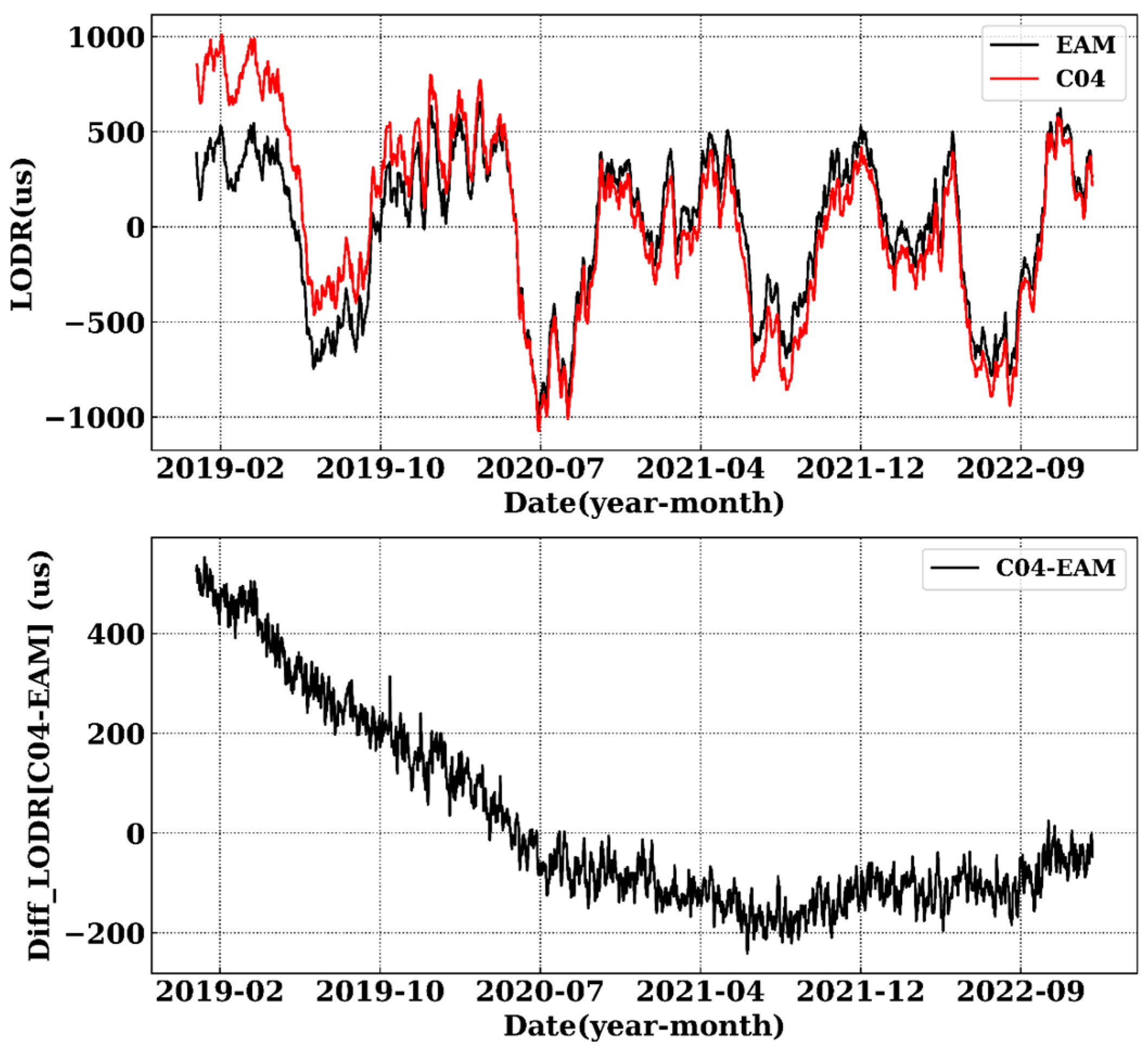
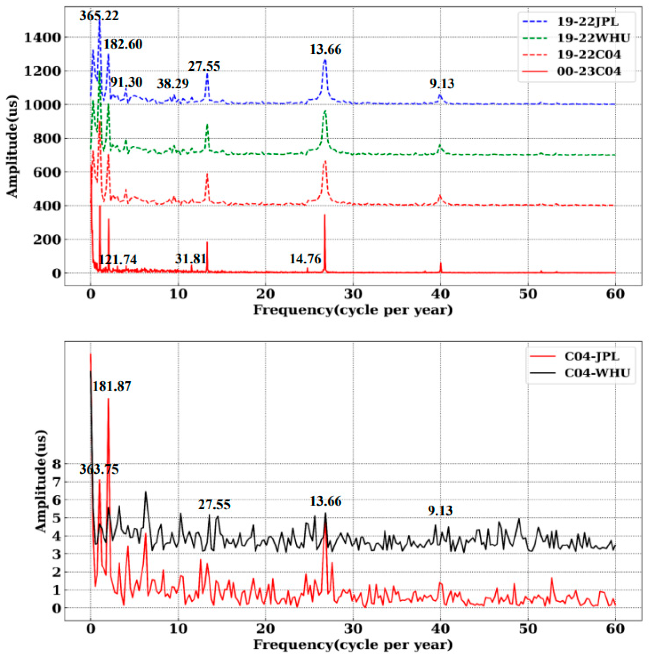
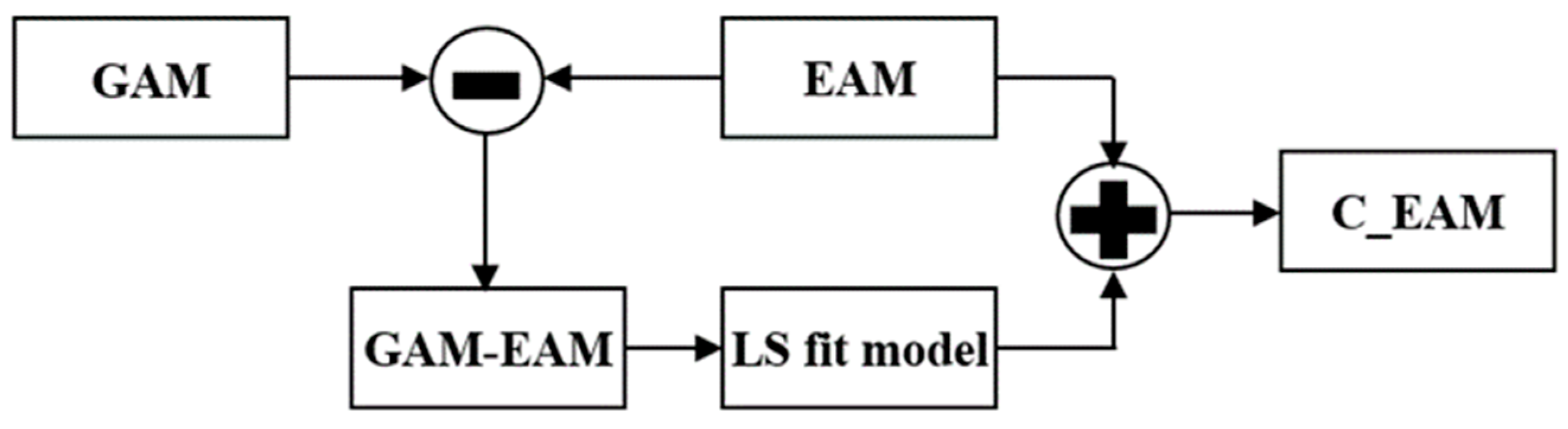
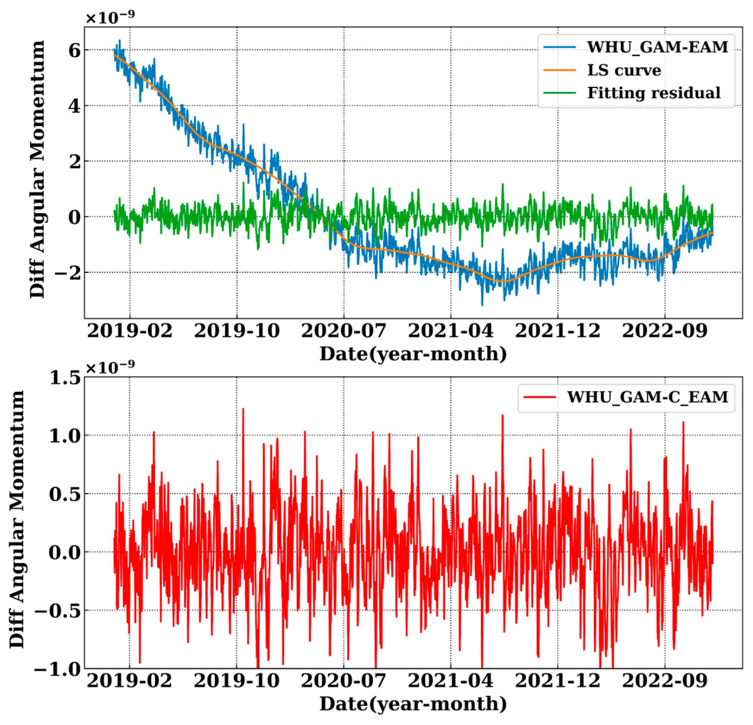
3.1.2. Differences Between EAM and LODR

The LOD series of the JPL and WHU from 2019 to 2022 were firstly converted to the geodetic angular momentum (GAM) using the axial Liouville equation, and then the EAM was subtracted. Dill et al. [41]’s spectra analysis of the GAM-EAM series shows six harmonic components, with periods of 9.1, 13.7, and 27.4 days and one-third of a year, one-half of a year, and one year. Here, we fit the GAM-EAM series by taking into account the three long-term (one-third of a year, one-half of a year, and one year) harmonic components. The differences between the EAM and GAM were then fitted with the formula that is presented in Equation (3). The linear components were fitted every year. Finally, the EAM was corrected using the least-square fitting model, denoted as C_EAM hereafter. Figure 5 shows the scheme we used to derive the C_EAM. The upper panel of Figure 6 shows the fitting of the long-term trend of the GAM-EAM; the lower panel of Figure 6 shows the differences between the C_EAM and GAM. The C_EAM series was then converted into the LODR domain, denoted as the LODRE hereafter, and was used as the input in the next step of the Kalman combination.

$$f_{GAM-EAM}(t)=\left.\left\{\begin{array}{l}{a}_0+a_{1}t\\ a_2+a_{3}t\\ a_4+a_{5}t\\ a_6+a_{7}t\end{array}\right.\right\}+\underset{i=1}{\overset{n}{\Sigma }}\left[c_i\sin ({\displaystyle \frac{2\pi t}{T_i}})+d_i\cos ({\displaystyle \frac{2\pi t}{T_i}})\right]$$

(3)

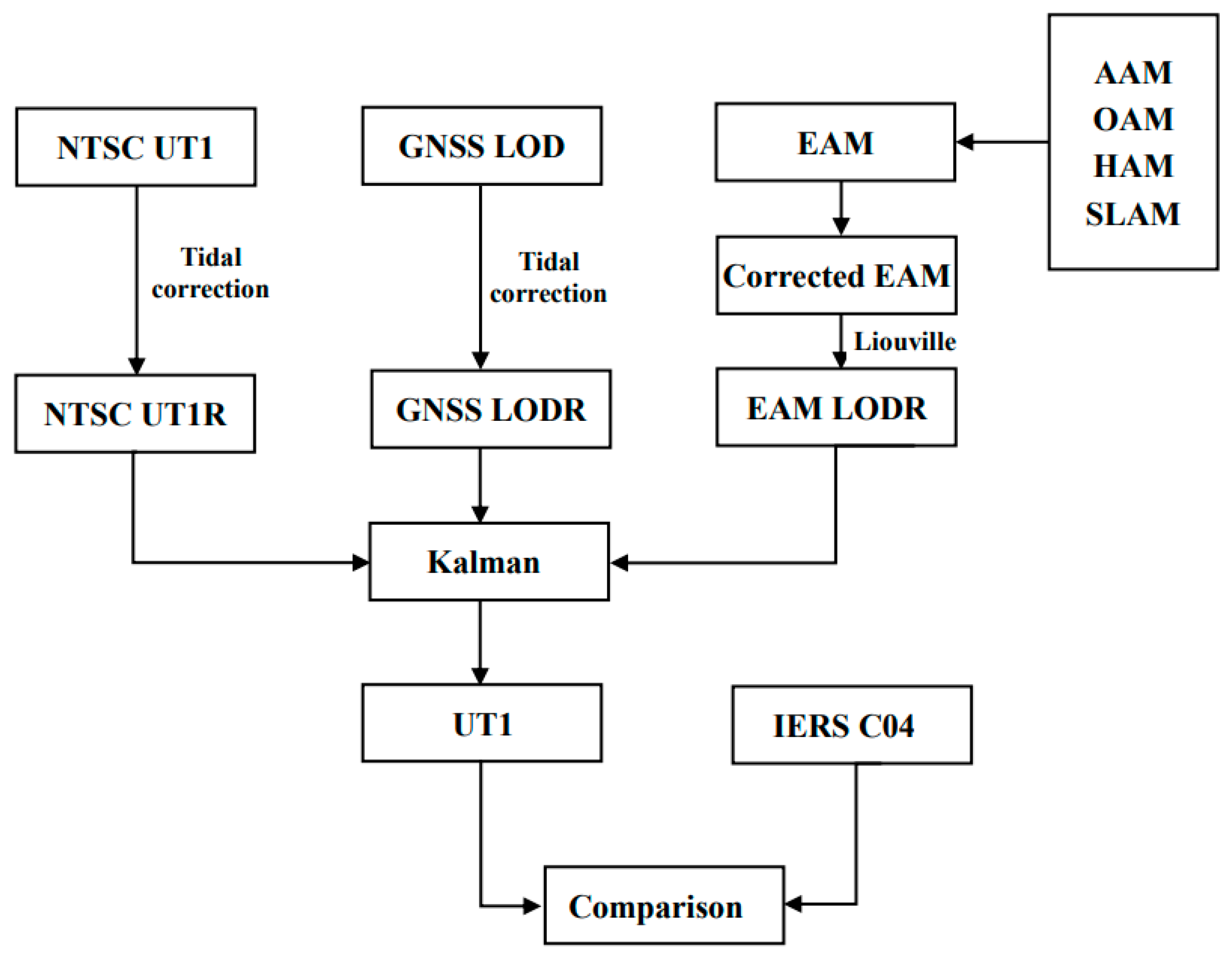
3.2. Kalman Combination Algorithm

The Kalman algorithm has proven to be an effective method for EOP combinations. The JPL group has long used the Kalman filter for EOP combinations [50,51]. Kehm et al. [21] pointed out that JPL COMB 2018 is considered one of the benchmark products concerning ERP accuracy. In this study, we designed an 11-parameter Kalman filter to combine the VLBI UT1R, GNSS LODR, and LODRE datasets. The LODRE was converted from the corrected EAM(C_EAM), as discussed in Section 3.1.2. The Kalman algorithm is as follows:

$$\begin{array}{l}{Z}_v(k)=H_{v}X(k)+V_v(k)\\ Z_g(k)=H_{g}X(k)+V_g(k)\\ Z_e(k)=H_{e}X(k)+V_e(k)\end{array}$$

(4)

The observation equations for the VLBI UT1R, GNSS LODR, and LODRE are presented in descending order. Among them, $H_v$, $H_g$, and $H_e$ are the observation matrices of the VLBI UT1R, GNSS LODR, and LODRE, respectively; $V_v(k)$, $V_g(k)$, and $V_e(k)$ represent the observation noise of the three measurements at time ($k$):

$$\begin{array}{l}{H}_v=[\begin{array}{ccccccccccc}1& 0& 0& 1& 0& 0& 0& 0& 0& 0& 0\end{array}]\\ H_g=[\begin{array}{ccccccccccc}0& 1& 0& 0& 1& 0& 0& 0& 0& 0& 0\end{array}]\\ H_e=[\begin{array}{ccccccccccc}0& 0& 1& 0& 1& 0& 0& 0& 0& 0& 0\end{array}]\end{array}$$

(5)

The equation of the state is as follows:

$$X(k)=FX(k-1)+W(k-1)$$

(6)

The state vector and state transition matrix are given in Equations (7) and (8):

$$X(k)=\left[\begin{array}{l}UT1R\\ LODR\\ LODRE\\ M_u\\ M_l\\ A\\ B\\ C\\ D\\ E\\ F_f\end{array}\right]$$

(7)

$$F=\left[\begin{array}{ccccccccccc}1& -a& -(1-a)& 0& 0& 0& 0& 0& 0& 0& 0\\ 0& 1& 0& 0& 0& {\beta }_1& {\beta }_2& {\beta }_3& {\beta }_4& {\beta }_5& {\beta }_6\\ 0& 0& 1& 0& 0& {\beta }_1& {\beta }_2& {\beta }_3& {\beta }_4& {\beta }_5& {\beta }_6\\ 0& 0& 0& 1& 0& 0& 0& 0& 0& 0& 0\\ 0& 0& 0& 0& 1& 0& 0& 0& 0& 0& 0\\ 0& 0& 0& 0& 0& 1& 0& 0& 0& 0& 0\\ 0& 0& 0& 0& 0& 0& 1& 0& 0& 0& 0\\ 0& 0& 0& 0& 0& 0& 0& 1& 0& 0& 0\\ 0& 0& 0& 0& 0& 0& 0& 0& 1& 0& 0\\ 0& 0& 0& 0& 0& 0& 0& 0& 0& 1& 0\\ 0& 0& 0& 0& 0& 0& 0& 0& 0& 0& 1\end{array}\right]$$

(8)

where

$$\begin{array}{l}{\beta }_1=\cos ({\displaystyle \frac{2\pi k}{9.13}}),{\beta }_2=\sin ({\displaystyle \frac{2\pi k}{9.13}}),{\beta }_3=\cos ({\displaystyle \frac{2\pi k}{13.66}}),\\ {\beta }_4=\sin ({\displaystyle \frac{2\pi k}{13.66}}),{\beta }_5=\cos ({\displaystyle \frac{2\pi k}{27.55}}),{\beta }_6=\sin ({\displaystyle \frac{2\pi k}{27.55}})\end{array}$$

(9)

In the Kalman filter design, we incorporated the systematic biases and periodic components derived from the analysis in Section 3.1.1 to better eliminate the effects of systematic errors and periodic terms, thereby achieving enhanced combination results. $M_{\mu }$ is the systematic bias of the UT1R, $M_l$ is the systematic bias of the LODR (i.e., the 33.92 µs and 20.17 µs biases for the JPL and WHU LODR series), and $A,B,C,D,E,F_f$ are the estimated coefficients of the three periodic components with periods of 9.13, 13.66, and 27.55 days. Here, we only took into account three components with periods less than 30 days, since this Kalman filter is used for rapid UT1 estimation. Here, $a$ and (1 − $a$) represent the weights of the LODR and LODRE. The priori of $a$ is calculated as the error of the LODRE/the errors of the LODR + the errors of the LODRE. The error of the LODR is the STD of the GNSS LODR, and the error of the LODRE is the STD of the LODRE. Since the diagonal elements of the covariance matrix represent the square of the uncertainty of the state estimation, after the first loop of the Kalman program, the value of $a$ is iteratively adjusted using the covariance matrix (P). The value of $a$ converges to a typical value of 0.505 after two–three iterations. $W(k)$ and $V(k)$ are uncorrelated white noise with variances of Q and $R$. R and Q are important parameters of the Kalman filter that affect the combination performance and are closely related to the covariance matrix of the Kalman filter and influence its estimation error. The value of the R matrix reflects the precision of the observed data itself. In this paper, we obtained the R matrix based on the statistics of the derived accuracy. As for the Q matrix, we referred to the research conducted by Morabito et al. [50] and Freedman et al. [33] on the modeling and analysis of the UT1 and LOD, as well as the AAM-LOD. In their studies, a random-walk model with the white noise stochastic process was used for the UT1/LOD, with a power spectral density of 0.0036 ms²/d³. For the AAM, a white noise stochastic process with a power spectral density of 0.004 ms²/d³ was adopted. The prediction equation and correction equation are as follows:

$$\begin{array}{cc}\hfill X(k/k-1)=& FX(k-1/k-1)\hfill \\ \hfill X(k/k)=& X(k/k-1)+K(k)(Z(k)\hfill \\ \hfill \hspace{0.25em}& -HX(k/k-1))\hfill \end{array}$$

(10)

where $X(k/k-1)$ represents the predicted state value at time ($k$), $X(k/k)$ represents the final state estimation value of the Kalman filter at time ($k$), and $K(k)$ is the Kalman gain used to adjust the observed and predicted values. The expression of $K(k)$ is given in Equation (11):

$$K(k)=P(k/k-1)H^T/(HP(k/k-1)H^T+R)$$

(11)

where $P(k/k-1)$ represents the covariance matrix of $X(k/k-1)$, and $R$ is the covariance matrix of the observed noise:

$$\begin{array}{l}P(k/k-1)=FP(k-1/k-1)F^T+Q\\ P(k/k)=(1-K(k)HP(k/k-1)\end{array}$$

(12)

$P(k/k)$ represents the covariance matrix of $X(k/k)$, and $Q$ represents the covariance matrix of state noise. $P(k/k)$ is a symmetric matrix, and its diagonal elements represent the variance in each state estimator, representing the expected square of the error between the true value and the filtered value. The square root of these elements is the uncertainty of the Kalman filter estimation:

$$Uncertainties=\sqrt{P_{ii}(k/k)}$$

(13)

$P_{ii}(k/k)$ represents the diagonal elements of the covariance matrix.

Mathematically, the Kalman filter program can run in both the forward and backward directions. We processed our data in both the forward and backward modes, which produced very consistent results. The final values we adopted are the averages of the forward and backward Kalman filter outputs.

4. Evaluation

With the UT1, LOD, and EAM datasets given in Section 2 and the combination method given in Section 3, we produced the combined series of both the UT1 and LOD, as shown in Figure 7.

First, tidal corrections were applied to the NTSC UT1 and GNSS LOD to obtain the NTSC UT1R and GNSS LODR. Then, the GNSS LODR (converted via the Liouville equation) was used to correct the EAM dataset. Subsequently, the corrected EAM was transformed using the Liouville equation to derive the EAM LODR. Finally, the Kalman combination was performed on the NTSC UT1R, GNSS LODR, and EAM LODR, and the combination accuracy was assessed.

In this section, we evaluate the accuracy of the Kalman combined series via a comparison with the C04 UT1/LOD series. Since the Kalman filter also estimates the uncertainty of the UT1 and LOD, the validation of the uncertainty is also presented.

4.1. Comparison with C04 UT1/LOD

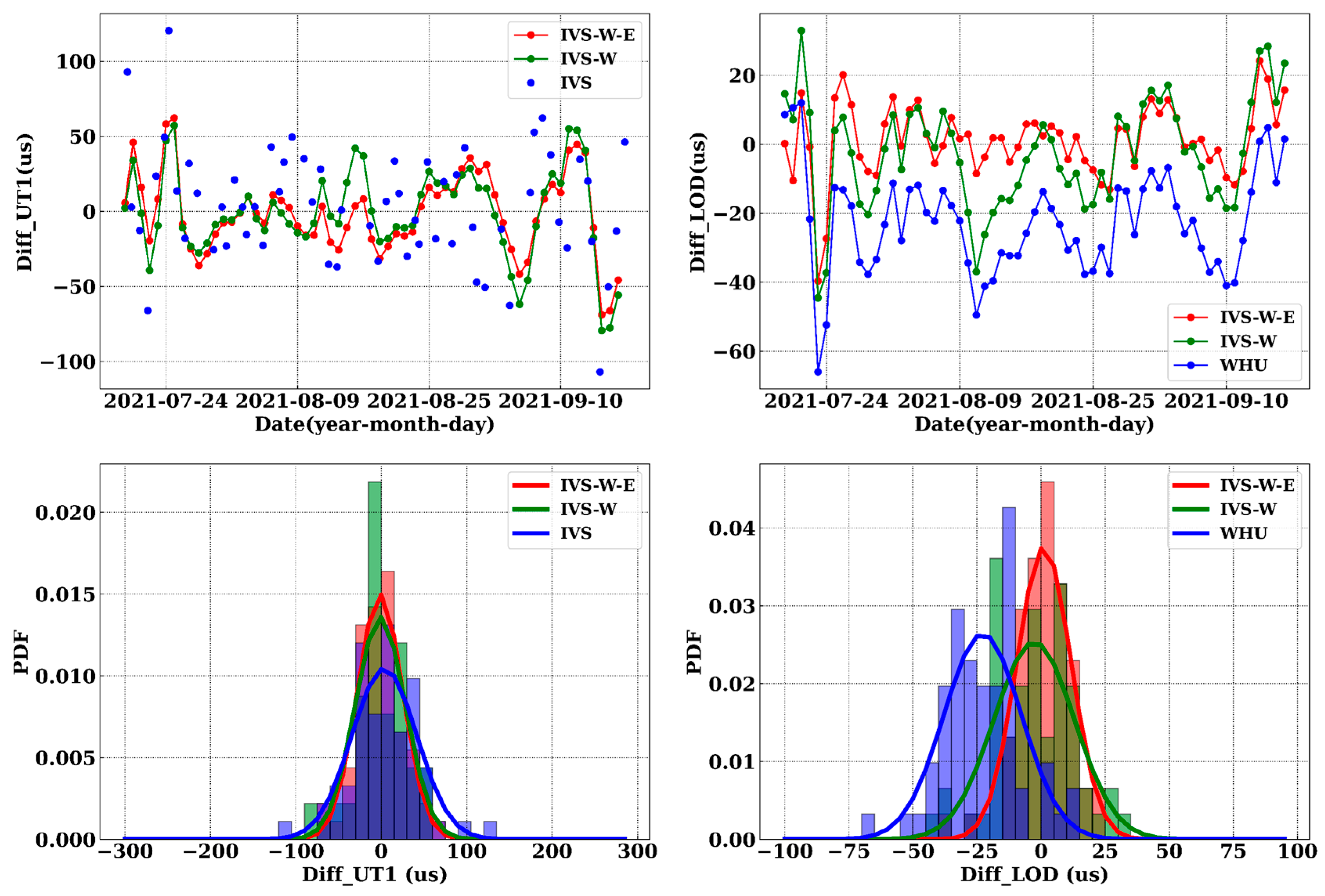
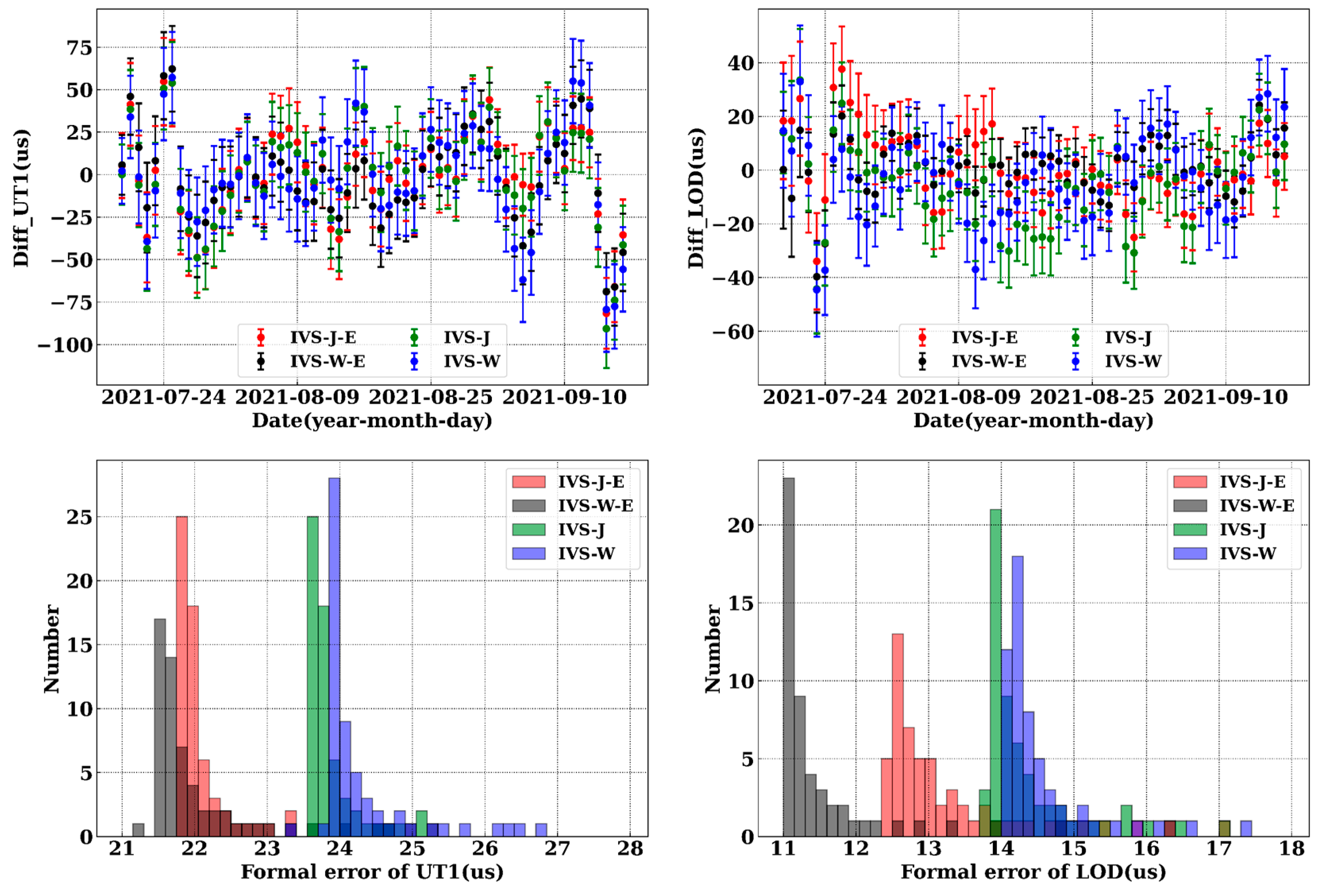
4.1.1. Combination of IVS with JPL/WHU and EAM

Figure 8 and Figure 9 show the differences between the Kalman combined UT1 (left panels) and LOD (right panels) with respect to the IERS C04. The only difference between Figure 8 and Figure 9 is the input LOD series, which is from the JPL for Figure 8 and from WHU for Figure 9. The blue dots in the upper left panel represent the difference between the IVS UT1 and IERS C04. The green line represents the difference between the combined UT1 using IVS UT1 and LOD data and IERS C04. The red line represents the difference between the combined UT1 using IVS UT1, LOD, and EAM data and IERS C04. The bottom left panel is a histogram that represents the distribution of the differences shown in the top left panel. The distributions of the three types of differences all follow normal distribution. The blue, green, and red lines are the normal-distribution curves, with the fitted mean and standard deviation listed in

Table 5. Statistics of combined UT1 and LOD. IVS-J-E means the combination of the IVS UT1, JPL LOD, and EAM. IVS-W-E means the combination of the IVS UT1, WHU LOD, and EAM. IVS-J means the combination of the IVS UT1 and JPL LOD. IVS-W means the combination of the IVS UT1 and WHU LOD.

UT1	RMS (µs)	STD (µs)	MEAN (µs)	MEDIAN (µs)	MAX. (µs)	MIN. (µs)
IVS-J-E	26.97	26.97	0.05	2.52	54.74	−81.68
IVS-W-E	26.67	26.64	−1.40	−1.46	62.24	−68.90
IVS-J	28.17	28.17	−0.09	2.38	54.00	−90.65
IVS-W	28.37	28.35	−1.08	−3.18	57.18	−79.45
IVS	38.33	38.16	3.61	2.91	120.38	−106.95
LOD	RMS (µs)	STD (µs)	MEAN (µs)	MEDIAN (µs)	MAX. (µs)	MIN. (µs)
IVS-J-E	13.54	13.48	1.35	−1.45	37.59	−33.93
IVS-W-E	10.68	10.62	1.12	1.81	24.18	−39.66
IVS-J	15.28	15.12	−2.23	0..03	36.48	−41.25
IVS-W	15.37	15.14	−2.71	−2.20	32.92	−44.52
JPL	45.41	15.16	−42.81	−43.7	−2.70	−85.00
WHU	27.35	15.11	−22.79	−22.30	12.00	−66.00

. The right panels are identical to the left panels in terms of content but are for the LOD. The statistics of Figure 8 and Figure 9, including the RMS, STD, mean, median, maximum, and minimum of the differences, are listed in Table 5. In the first column of Table 5, W denotes WHU, J denotes the JPL, and E denotes the EAM. IVS-J-E means the combination of the IVS UT1, JPL LOD, and EAM, and IVS-W-E means the combination of the IVS UT1, WHU LOD, and EAM.

In Figure 8 and Figure 9, the combination of the UT1 series is presented. The RMS error of the IVS UT1 series was 38.33 µs, which decreased to 26.97 µs and 26.67 µs after combination with the JPL and WHU LOD series, respectively, representing improvements in accuracy of 29.64% and 30.42%. The maximum deviation decreased from ~120.38 µs to ~54.74 µs, and the minimum deviation decreased from ~ −105.95 µs to ~−68.90 µs. Another improvement was observed in the RMS error of the LOD. The RMS of the JPL LOD series was 45.41 µs, which decreased to 13.54 µs, indicating an enhancement in accuracy of 70.18%. The RMS of the WHU LOD was 27.35 µs, which decreased to 10.68 µs, showing an improvement in accuracy of 60.95%. By incorporating the EAM data, the RMS of the combined UT1 was reduced by 1.20 µs when the JPL LOD was used as the input, and by 1.70 µs when the WHU LOD was the input; the RMS of the combined LOD for WHU was also reduced by 4.69 µs, and for the JPL, by 1.74 µs. Generally, with the EAM dataset, the accuracy of the UT1 was enhanced by 4–6%, and the accuracy of the LOD was improved by 11–30%.

In addition, we confirmed that the system bias term Ml estimated by the Kalman combination algorithm agreed with the bias value of the LOD w.r.t. C04 series for both the JPL and WHU datasets. This verified the capability of the Kalman filter for the calibration of the LOD with UT1 data.

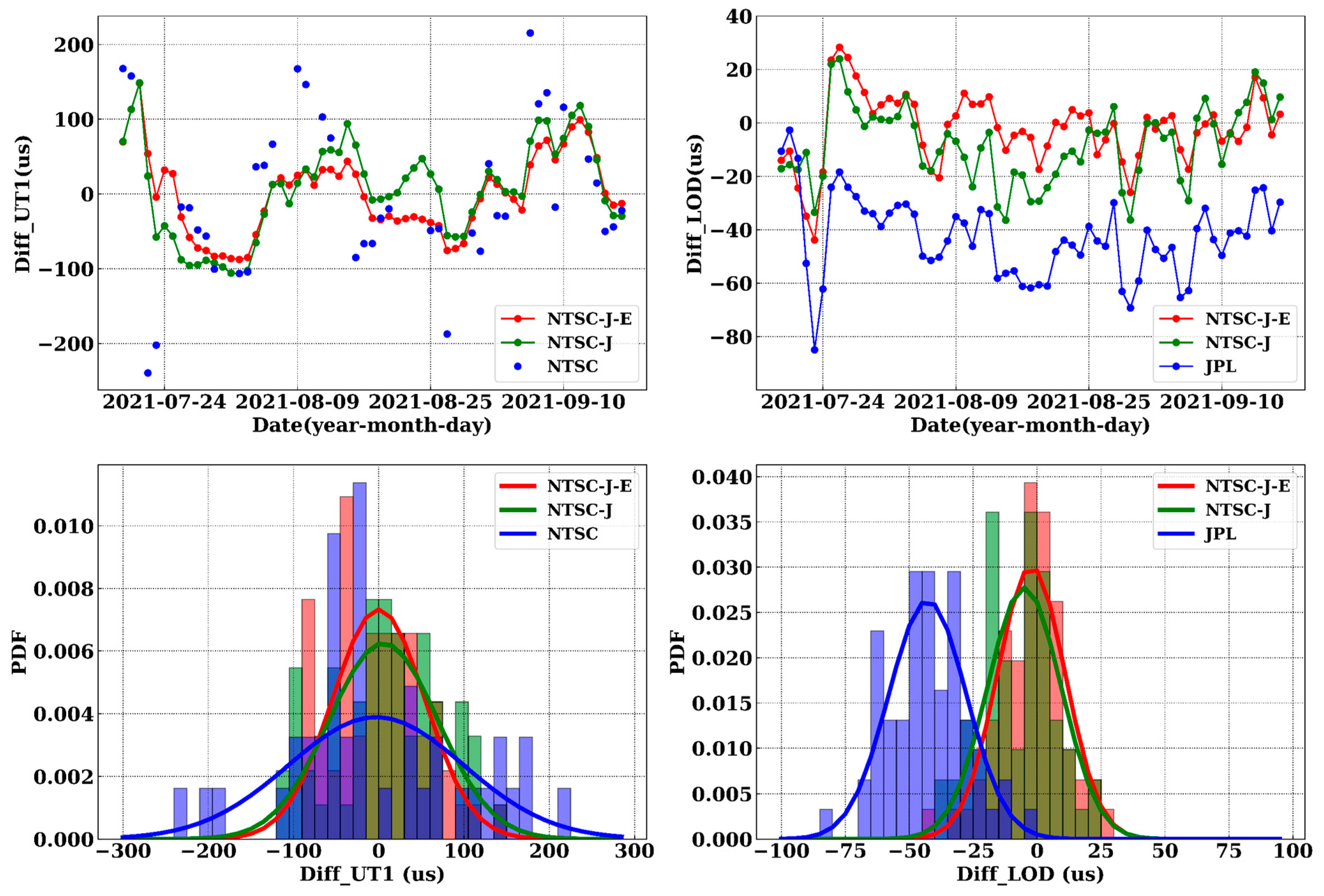
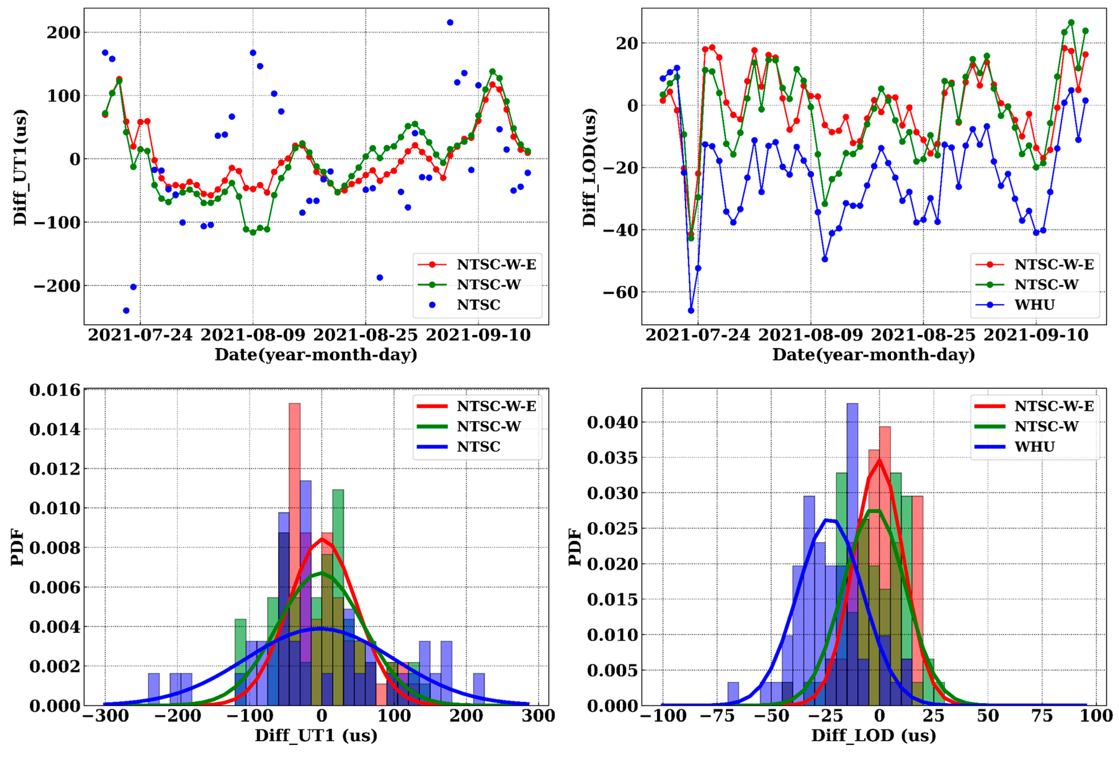
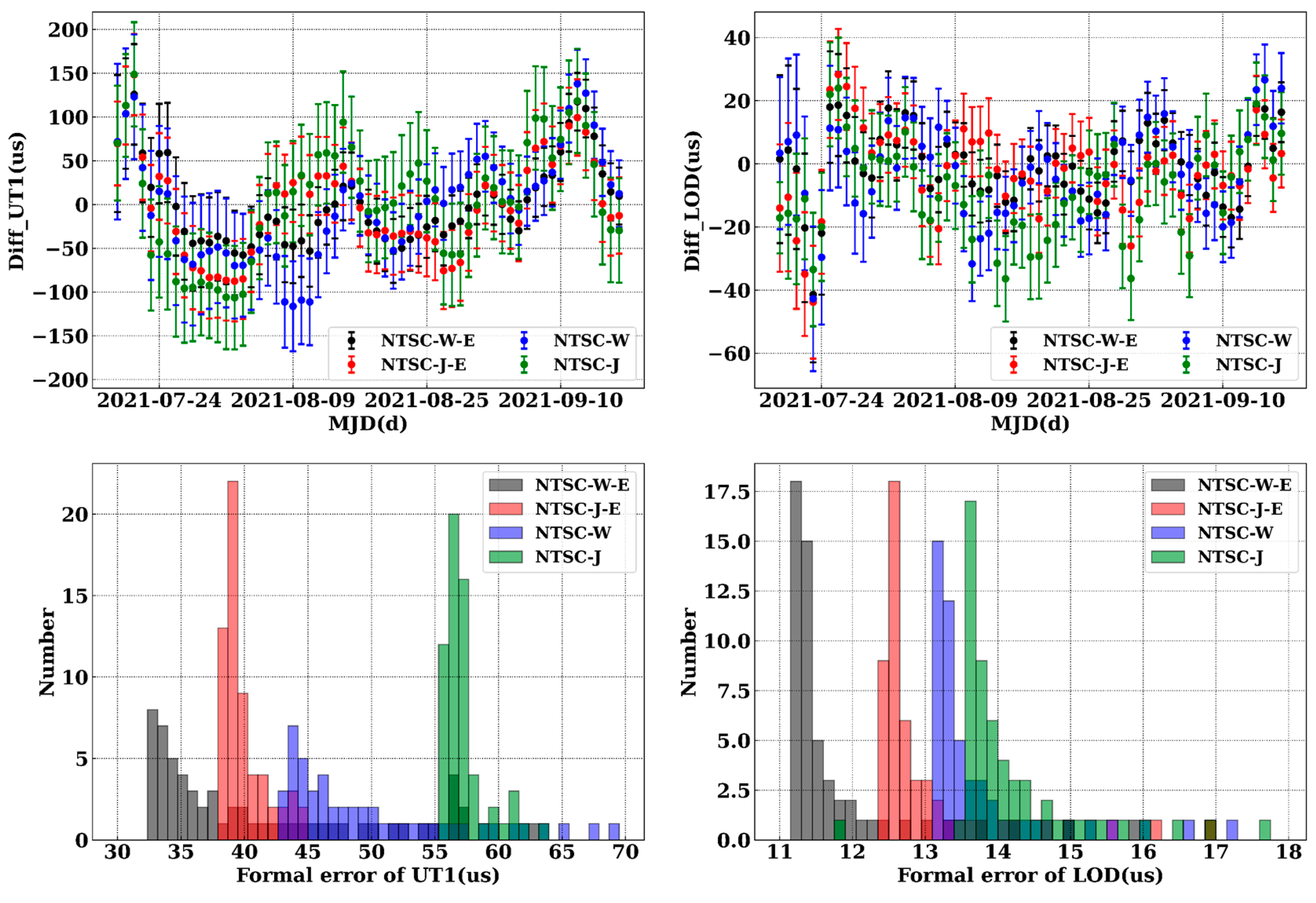
4.1.2. Combination of NTSC with JPL/WHU and EAM

Figure 10 and Figure 11 are similar to Figure 8 and Figure 9, with the only difference being that the IVS input dataset is replaced with the NTSC input dataset. Figure 10 and Figure 11 show the combined UT1 and LOD with the NTSC UT1 series as the input. The statistics of Figure 10 and Figure 11, including the RMS, STD, mean, median, maximum, and minimum of the differences, are listed in

Table 6. Statistics of combined UT1 and LOD. NTSC-J-E means the combination of the NTSC UT1, JPL LOD, and EAM. NTSC-W-E means the combination of the NTSC UT1, WHU LOD, and EAM. NTSC-J means the combination of the NTSC UT1 and JPL LOD. NTSC-W means the combination of the NTSC UT1 and WHU LOD.

UT1	RMS (µs)	STD (µs)	MEAN (µs)	MEDIAN (µs)	MAX. (µs)	MIN. (µs)
NTSC-J-E	54.42	54.42	−0.13	−3.86	148.24	−87.67
NTSC-W-E	47.36	47.35	1.02	−14.49	125.80	−57.78
NTSC-J	64.09	63.86	5.51	6.27	148.55	−106.55
NTSC-W	59.49	59.46	−1.79	3.60	137.84	−116.36
NTSC	102.69	102.65	−3.00	−22.20	215.30	−239.60
LOD	RMS (µs)	STD (µs)	MEAN (µs)	MEDIAN (µs)	MAX. (µs)	MIN. (µs)
NTSC-J-E	13.47	13.27	−2.28	−1.38	28.29	−43.84
NTSC-W-E	11.54	11.53	−0.48	0.40	18.59	−41.44
NTSC-J	14.68	14.38	−2.98	−0.73	28.99	−31.43
NTSC-W	14.55	14.33	−2.49	−1.08	26.60	−42.76
JPL	45.41	15.16	−42.81	−43.7	−2.70	−85.00
WHU	27.35	15.11	−22.79	−22.30	12.00	−66.00

. In the first column of Table 6, NTSC-J-E means the combination of the NTSC UT1, JPL LOD, and EAM, and NTSC-W-E means the combination of the NTSC UT1, WHU LOD, and EAM. The combinations produced a continuous UT1 series with improved accuracy. The RMS error of the NTSC UT1 series was 102.69 µs, which was reduced to 54.42 and 47.36 µs after combination with the JPL and WHU LOD series, respectively, indicating improvements in accuracy of 47.01% and 53.88%. The maximum deviation was decreased from ~215.30 µs to ~125.80 µs, and the minimum deviation was lowered from ~−239.60 µs to ~−57.78 µs.

The RMS of the LOD of the JPL series was 45.41 µs, which decreased to 13.47 µs, indicating an improvement in accuracy of 70.33%. The RMS of the WHU LOD was 27.35 µs, which decreased to 11.54 µs, showing an enhancement in accuracy of 57.81%. After incorporating the EAM data, the RMS of the combined UT1 was reduced by 9.67 µs when the JPL LOD was used as the input, and by 12.13 µs when the WHU LOD was the input; the RMS of the combined LOD was also reduced by 3.01 µs for the WHU LOD, and by 1.21 µs for the JPL LOD. In summary, with the assistance of the EAM dataset, the accuracy of the UT1 was enhanced by 15–20%, and the accuracy of the LOD was improved by 8–21%.

A comparison of the RMSs in Table 5 and Table 6 of the UT1 with and without the aid of the EAM dataset indicates that the EAM dataset can effectively improve the UT1, especially for UT1 inputs with large RMSs.

4.2. UT1/LOD Uncertainty

To further assess the reliability of the proposed algorithm, a comprehensive investigation into the uncertainties associated with the UT1 and LOD was conducted. These uncertainties were estimated as the square root of the diagonal elements of the covariance matrix.

In Figure 12 and Figure 13, the upper panels illustrate the scatter plots of the combined UT1 and LOD values in comparison to the C04 reference values, with the Kalman-estimated uncertainties depicted as error bars. Notably, in these figures, the error bars signify the 1-sigma (65%) confidence intervals. The bottom panels present the histograms of the uncertainties estimated by the Kalman filter for the UT1 (left panels) and LOD (right panels). In

Table 7. Statistics of RMS w.r.t. C04 and Kalman-estimated uncertainties.

PRODUCT	UT1/µs		LOD/µs
	RMS w.r.t. C04	Kalman Uncertainties	RMS w.r.t. C04	Kalman Uncertainties
IVS-J-E	26.97	22.30	13.54	13.92
IVS-W-E	26.67	21.92	10.68	11.03
IVS-J	28.17	24.70	15.28	14.70
IVS-W	28.37	24.27	15.27	14.12
NTSC-J-E	54.42	42.95	13.47	12.59
NTSC-W-E	47.36	35.47	11.54	11.12
NTSC-J	64.09	55.22	14.68	14.29
NTSC-W	59.49	49.81	14.55	13.92

, we tabulated the RMS values of the combined UT1 and LOD series, along with the mean uncertainties calculated using the Kalman filter. It was observed that for the LOD, the RMS and the Kalman-estimated uncertainties were nearly identical within a tolerance of 1 µs. For the UT1, a significant positive correlation was identified between the RMS values relative to C04 and the Kalman-estimated uncertainties. Specifically, the RMS values ranged from 26 µs to 64 µs, while the Kalman uncertainties spanned from 21 µs to 55 µs. The Pearson correlation coefficient between the RMS of the LOD and the uncertainty of the Kalman estimation was determined to be 0.95, and for the UT1, this coefficient was 0.98. These findings clearly indicate that both the RMS and the Kalman uncertainties serve as effective indicators of the uncertainty and quality of the UT1 series.

5. Discussion

5.1. The Combination of IVS and NTSC UT1

We also carried out Kalman combination experiments by integrating the IVS and NTSC UT1 measurements as the UT1 inputs. The combined results of IVS + NTSC + WHU + EAM are shown in

Table 8. Statistics of combined UT1 and LOD (IVS + NTSC + WHU + EAM).

UT1	RMS (µs)	STD (µs)	MEAN (µs)	MEDIAN (µs)	MAX. (µs)	MIN. (µs)
IVS-NTSC-W-E	25.59	25.49	2.22	3.34	59.42	−59.54
IVS-W-E	26.67	26.64	−1.40	−1.46	62.24	−68.90
IVS-NTSC	39.43	39.08	5.18	2.35	90.34	−95.70
IVS	38.33	38.16	3.61	2.91	120.38	−106.95
LOD	RMS (µs)	STD (µs)	MEAN (µs)	MEDIAN (µs)	MAX. (µs)	MIN. (µs)
IVS-NTSC-W-E	10.77	10.77	−0.08	0.23	22.69	−42.93
IVS-W-E	10.68	10.62	1.12	1.81	24.18	−39.66
WHU	27.35	15.11	−22.79	−22.30	12.00	−66.00

.

In Table 8, it can be seen that the RMS and STD of the IVS + NTSC + WHU + EAM combined UT1 are slightly better than those of the IVS + WHU + EAM. This indicates that more frequent UT1 measurements lead to a more stable result. The relatively small improvement might be attributed to the fact that the NTSC dataset has approximately 2 times lower accuracy and 3 times lower frequency compared to the IVS dataset, which results in less significant enhancements in the combined results. In terms of the LOD, adding the NTSC UT1 does not improve the LOD accuracy remarkably, but it slightly reduces the systematic bias of the LOD.

It should be noted that the reference dataset used in our evaluation was the 20 C04 series. To validate the applicability of our results, we assessed the differences between the NTSC UT1, IVS UT1, and UT1 values from both the 14 C04 and 20 C04 series for the period 2021–2023. The results demonstrate that using either the 20 C04 or 14 C04 series has minimal impact on the accuracy assessment of the UT1, indicating that both versions can serve as reliable reference datasets for UT1 precision comparisons.

5.2. Time Resolution of Input Datasets

Currently, both the GNSS and EAM are capable of providing routine updates daily or even more frequently. For example, the GNSS rapid ERP product is updated at 12:00 (UT). The time resolutions of the AAM, OAM, HAM, and SLAM within the EAM are not exactly the same: the AAM and OAM are updated every 3 h, while the HAM and SLAM are updated every 24 h at UT = 12:00. IVS intensive observations are almost available every day. Specifically, the INT1 is observed for 1 hour starting from 18:30 (UT) from Monday to Friday, the INT2 is observed for 1 h starting from 7:30 (UT) on Saturdays and Sundays, and the INT3 is observed for 1 hour starting from 7:00 (UT) every Monday. The NTSC started commissioning UT1 observations from 2018 and began conducting routine intensive UT1 observations 2 times per week from June 2021. Recently, since March 2023, the observation frequency has been increased to 3 times per week, on Mondays, Tuesdays, and Thursdays at 18:00 (UT).

To simplify the design of the Kalman filter, we resampled all these input datasets to the time of UT = 0 h. For UT1/LOD inputs, we first removed their high-frequency tidal terms. Then, the tidal-free LOD series was interpolated to the time stamp of mjd = 0. For the tidal-free UT1 series, if the decimal part of mjd < 0.5, we interpolated UT1 values to the nearest time stamp of mjd = 0; if the decimal part of mjd > 0.5, we extrapolated the UT1 to the nearest time stamp of mjd = +1 day. The AAM and OAM datasets with a time resolution of 3 h were smoothed to 1-day interval series at the time stamp of mjd = 0 using a smooth kernel provided by Dr. Dill of GFZ. If there was a missing value of the UT1/LOD/EAM at a given time, we used the Kalman-estimated UT1/LOD/EAM value from the previous time as the output. Through this approach, we were able to generate combined UT1, LOD, and EAM series with a 1-day time interval, all at the time stamp of UT = 0 h.

It should be noted that the Kalman algorithm is a recursive algorithm based on time series, where the state prediction and update steps rely on the consistency of time intervals. If the time intervals are inconsistent, the calculations can become complex and even inaccurate. Therefore, the Kalman algorithm requires a high degree of continuity in the dataset when applied.

5.3. Prospects

Based on the evaluations of the Kalman filter using different datasets, we propose the following prospects:

(a)

The development of an updated Kalman filter with the ability to handle multiple UT1, LOD, and EAM inputs, which can be used to combine and evaluate more UT1, LOD, and EAM results from multiple analysis centers;

(b)

The design of a Kalman filter tool that can also integrate the polar motion components with the VLBI, GNSS, and EAM datasets as inputs (the X and Y components of the AAM show strong correlation and consistent periodicity with the PMX and PMY, respectively);

(c)

Investigations and estimations of the uncertainties of the EAM dataset to enhance the combination and prediction of EOPs.

6. Conclusions

Due to the high correlation between AAM data and LOD data, and their widespread application in UT1/LOD forecasting, this study introduced the EAM into the UT1 combination to further enhance its accuracy. We designed an 11-parameter Kalman filter to combine the UT1 and LOD series with the aid of EAM data. In the state vector and state transition matrix, the system biases and periodic terms of the LOD and EAM datasets are taken into account. First, Fourier analysis was employed to preprocess the systematic biases and periodicity of the WHU/JPL LOD datasets. Second, the GAM data derived from WHU/JPL were used to correct the EAM. Finally, the UT1 data combination from three techniques was achieved, and the uncertainty was evaluated, resulting in a UT1 sequence with higher accuracy, better continuity, and stronger stability. The main conclusions are as follows:

(a)

The 11-parameter combination algorithm improved the accuracy of the UT1 data by over 30%, with the accuracy of the UT1 dataset from the NTSC increasing by nearly 54%, and the accuracy of the intensive observation UT1 dataset from the IVS improving by approximately 30%;

(b)

Compared to using only the GNSS and VLBI datasets, the inclusion of the EAM dataset yields superior combination results, characterized by higher accuracy, better stability, and more concentrated outcomes. Particularly for UT1 input datasets with high uncertainty, the EAM dataset can enhance the UT1 combination accuracy by 10 µs;

(c)

The formal uncertainty, measured by the square root of the diagonal elements of the covariance matrix, demonstrates that the Kalman combination model exhibits high reliability and rationality;

(d)

Validation through eight combination scenarios confirmed the algorithm’s strong applicability to input datasets. The higher the accuracy of the input dataset, the greater the combination accuracy; for datasets with lower accuracy, the improvement is more pronounced;

(e)

The combination algorithm not only corrects the systematic biases in the LOD but also effectively enhances the accuracy of LOD data.

References

1. Petti, G.; Luzum, B. IERS Conventions 2010; Verlag des Bundesamts für Kartographie und Geodäsie: Frankfurt am Main, Germany, 2010; Available online: https://www.researchgate.net/publication/235112142 (accessed on 1 January 2025)ISBN 3-89888-989-6.
2. Gambis, D.; Luzum, B. Earth rotation monitoring, UT1 determination and prediction. Metrologia 2011, 48, 165–170. [Google Scholar] [CrossRef]
3. Nastula, J.; Chin, T.M.; Gross, R.; Śliwińska, J.; Wińska, M. Smoothing and predicting celestial pole offsets µsing a Kalman filter and smoother. J. Geod. 2020, 94, 2–17. [Google Scholar] [CrossRef]
4. Nilsson, T.; Böhm, J.; Schuh, H. Sub-diurnal earth rotation variations observed by VLBI. Artif. Satell. 2010, 45, 49–55. [Google Scholar] [CrossRef]
5. Nilsson, T.; Böhm, J.; Schuh, H. Universal time from VLBI single-baseline observations during CONT08. J. Geod. 2011, 85, 415–423. [Google Scholar] [CrossRef]
6. Nilsson, T.; Heinkelmann, R.; Karbon, M.; Raposo-Pulido, V.; Soja, B.; Schuh, H. Earth orientation parameters estimated from VLBI during the CONT11 campaign. J. Geod. 2014, 88, 491–502. [Google Scholar] [CrossRef]
7. Byram, S.; Hackman, C. High-precision GNSS orbit, clock and EOP estimation at the United States Naval Observatory. In Proceedings of the 2012 IEEE/ION Position, Location and Navigation Symposium, Myrtle Beach, SC, USA, 23–26 April 2012. [Google Scholar] [CrossRef]
8. Hein, G.W. Status, perspectives and trends of satellite navigation. Satell. Navig. 2020, 1, 22. [Google Scholar] [CrossRef]
9. Mireault, Y.; Kouba, J. IGS Earth rotation parameters. GPS Solut. 1999, 3, 59–72. [Google Scholar] [CrossRef]
10. Coulot, D.; Pollet, A.; Collilieux, X.; Berio, P. Global optimization of core station networks for space geodesy: Application to the referencing of the SLR EOP with respect to ITRF. J. Geod. 2010, 84, 31–50. [Google Scholar] [CrossRef]
11. Pavlov, D. Role of lunar laser ranging in realization of terrestrial, lunar, and ephemeris reference frames. J. Geod. 2020, 94, 5. [Google Scholar] [CrossRef]
12. Pearlman, M.R.; Degnan, J.J.; Bosworth, J.M. The international laser ranging service. Adv. Space Res. 2002, 30, 135–143. [Google Scholar] [CrossRef]
13. Willis, P.; Fagard, H.; Ferrage, P.; Lemoine, F.G.; Noll, C.E.; Noomen, R.; Otten, M.; Ries, J.C.; Rothacher, M.; Soudarin, L.; et al. The international DORIS service (IDS): Toward maturity. Adv. Space Res. 2010, 45, 1408–1420. [Google Scholar] [CrossRef]
14. Moreaux, G.; Lemoine, F.G.; Capdeville, H.; Kuzin, S.; Otten, M.; Štěpánek, P.; Willis, P.; Ferrage, P. The international DORIS service contribution to the 2014 realization of the international terrestrial reference frame. Adv. Space Res. 2016, 58, 2479–2504. [Google Scholar] [CrossRef]
15. Angermann, D.; Seitz, M.; Drewes, H. Analysis of the DORIS contributions to ITRF2008. Adv. Space Res. 2010, 46, 1633–1647. [Google Scholar] [CrossRef]
16. Taller, D.; Krugel, M.; Rothache, M.; Tesmer, V.; Schmid, R.; Angermann, D. Combined Earth orientations parameters based on Homogeneous and continuous VLBI and GPS dhata. J. Geod. 2007, 81, 529–541. [Google Scholar] [CrossRef]
17. Bizouard, C.; Gambis, D. The combined solution C04 for Earth orientation parameters consistent with international terrestrial reference frame 2005. In Proceedings of the International Association of Geodesy Symposium, Munich, Germany, 9–14 October 2009; pp. 265–270. [Google Scholar] [CrossRef]
18. Artz, T.; Bernhard, L.; Nothnagel, A.; Steigenberger, P.; Tesmer, S. Methodology for the combination of sub-daily Earth rotation from GPS and VLBI observations. J. Geod. 2012, 86, 221–239. [Google Scholar] [CrossRef]
19. Bizouard, C.; Lambert, S.; Gattano, C.; Becker, O.; Richard, J.-Y. The IERS EOP 14C04 solution for Earth orientation parameters consistent with ITRF 2014. J. Geod. 2019, 93, 621–633. [Google Scholar] [CrossRef]
20. Ratcliff, J.T.; Gross, R.S. Combinations of Earth Orientation Measurements: SPACE2018, COMB2018, and POLE2018; JPL Publication 19-7; National Aeronautics and Space Administration: Washington, DC, USA, 2019; Available online: https://www.researchgate.net/publication/336778776 (accessed on 1 January 2025).
21. Kehm, A.; Hellmers, H.; Blossfeld, M.; Dill, R.; Angermann, D.; Seitz, F.; Hugentobler, U.; Dobslaw, H.; Thomas, M.; Thaller, D.; et al. Combination strategy for consistent final, rapid and predicted Earth rotation parameters. J. Geod. 2023, 97, 3. [Google Scholar] [CrossRef]
22. He, B.; Wang, X.Y.; Hu, X.G.; Zhao, Q.-H. Combination of terrestrial reference frames based on space geodetic techniques in SHAO: Methodology and main issues. Res. Astron. Astrophys. 2017, 17, 89. [Google Scholar] [CrossRef]
23. Schoenemann, E.; Springer, T.; Otten, M.; Mayer, V.; Bruni, S.; Enderle, W.; Zandbergen, R. Status of ESA’s independent Earth orientation parameter products. In Proceedings of the EGU General Assembly 2020, Online, 4–8 May 2020. EGU 2020-17154. [Google Scholar] [CrossRef]
24. Gambis, D.; Biancale, R.; Carlucci, T.; Lemoine, J.; Marty, J.; Bourda, G.; Charlot, P.; Loyer, S.; Lalanne, T.; Soudarin, L.; et al. Combination of Earth Orientation Parameters and Terrestrial Frame at the Observation Level. Int. Assoc. Geod. Symp. 2009, 134, 3–9. [Google Scholar] [CrossRef]
25. Wang, J.G.; Ge, M.R.; Glaser, S. Impact of Tropospheric Ties on UT1-UTC in GNSS and VLBI Integrated Solution of in tensive Sessions. J. Geophys. Res-Solid Earth 2022, 127, e2022JB025228. [Google Scholar] [CrossRef]
26. Davis, M.; Carter, M.S.; Dieck, C.; Stamatakos, N. The IERS Rapid Service/Prediction Centre UT1−UTC Combined Solution: Present and Future Contributions. In Proceedings of the 24th Meeting of the European VLBI Group for Geodesy and Astrometry, Las Palmas de Gran Canaria, Spain, 17–19 March 2019; pp. 184–189. [Google Scholar]
27. Schindelegger, M.; Bohm, J.; Salstein, D. High resolution atmospheric angular momentum functions related to Earth rotation parameters during CONT08. J. Geod. 2011, 85, 425–433. [Google Scholar] [CrossRef]
28. Hide, R.; Birch, N.T.; Morrison, L.V.; Shea, D.J.; White, A.A. Atmospheric angular momentum fluctuations and changes in the length of the day. Nature 1980, 286, 114–117. [Google Scholar] [CrossRef]
29. Eubanks, T.M.; Steppe, J.A.; Dickey, J.O.; Callahan, P.S. A spectral-analysis of the Earth’s angular momentum budget. J. Geophys. Res. 1985, 90, 5385–5404. [Google Scholar] [CrossRef]
30. Rosen, R.D.; Salstein, D.A.; Wood, T.M. Discrepancies in the Earth atmosphere angular momentum budget. J. Geophys. Res.-Solid Earth Planets 1990, 95, 265–279. [Google Scholar] [CrossRef]
31. Mound, J.E.; Buffett, B.A. Detection of a gravitational oscillation in length-of-day. Earth Planet. Sc. Lett. 2006, 243, 383–389. [Google Scholar] [CrossRef]
32. Niedzielski, T.; Kosek, W. Prediction of UT1–UTC, LOD and AAM by combination of least-squares and multivariate stochastic methods. J. Geod. 2008, 82, 83–92. [Google Scholar] [CrossRef]
33. Freedman, A.P.; Steppe, J.A.; Dickey, J.O.; Eubanks, T.M.; Sung, L.Y. The short-term prediction of universal time and length of day µsing atmospheric angular momentum. J. Geophys. Res. Solid Earth 1994, 99, 6981–6996. [Google Scholar] [CrossRef]
34. Gross, R.S.; Fukumori, I.; Menemenlis, D.; Gegout, P. Atmospheric and oceanic excitation of length-of-day variations during 1980–2000. J Geophys Res Solid Earth 2004, 109. [Google Scholar] [CrossRef]
35. Guo, J.Y.; Li, Y.B.; Dai, C.; Shum, C. A technique to improve the accuracy of Earth orientation prediction algorithms based on least squares extrapolation. J. Geodyn. 2013, 70, 36–48. [Google Scholar] [CrossRef]
36. Rekier, J.; Chao, B.F.; Chen, J.; Dehant, V.; Rosat, S.; Zhu, P. Earth’s Rotation: Observations and Relation to Deep Interior. Surv. Geophys. 2022, 43, 149–175. [Google Scholar] [CrossRef]
37. Li, X.; Yang, X.; Ye, R.; Cheng, X.; Zhang, S. Research on Methods to Improve Length of Day Precision by Combining with Effective Angular Momentum. Remote Sens. 2024, 16, 722. [Google Scholar] [CrossRef]
38. Li, X.; Wu, Y.; Yao, D.; Liu, J.; Nan, K.; Ma, L.; Cheng, X.; Yang, X.; Zhang, S. Research on UT1-UTC and LOD Prediction Algorithm Based on Denoised EAM Dataset. Remote Sens. 2023, 15, 4654. [Google Scholar] [CrossRef]
39. Nothnagel, A.; Schnell, D. The impact of errors in polar motion and nutation on UT1 determinations from VLBI intensive observations. J. Geod. 2008, 82, 863–869. [Google Scholar] [CrossRef]
40. Yao, D.; Wu, Y.W.; Zhang, B.; Sun, J.; Sun, Y.; Xu, S.-J.; Liu, J.; Ma, L.-M.; Gong, J.-J.; Yang, Y.; et al. The NTSC VLBI System and its application in UT1 measurement. Res. Astron. Astrophys. 2020, 20, 153–162. [Google Scholar] [CrossRef]
41. Dill, R.; Dobslaw, H.; Thomas, M. Improved 90-day Earth orientation predictions from angular momentum forecasts of atmosphere, ocean, and terrestrial hydrosphere. J. Geod. 2019, 93, 287–295. [Google Scholar] [CrossRef]
42. Dobslaw, H.; Dill, R.; Grötzsch, A.; Brzezinski, A.; Thomas, M. Seasonal polar motion excitation from numerical models of atmosphere, ocean, and continental hydrosphere. J. Geophys. Res. 2010, 115, 406. [Google Scholar] [CrossRef]
43. Jungclaus, J.H.; Fischer, N.; Haak, H.; Lohmann, K.; Marotzke, J.; Matei, D.; Mikolajewicz, U.; Notz, D.; von Storch, J.S. Characteristics of the ocean simulations in the Max Planck Institute Ocean Model (MPIOM) the ocean component of the MPI-Earth system model. J. Adv. Model. Earth Syst. 2013, 5, 422–446. [Google Scholar] [CrossRef]
44. Hagemann, S.; Dumenil, L. A parametrization of the waterflow for the global scale. Clim. Dyn. 1998, 14, 17–31. [Google Scholar] [CrossRef]
45. Tamisiea, M.E.; Hill, E.M.; Ponte, R.M.; Davis, J.L.; Velicogna, I.; Vinogradova, N.T. Impact of self-attraction and loading on the annual cycle in sea level. J. Geophys. Res-Oceans 2010, 115, 1–15. [Google Scholar] [CrossRef]
46. Dobslaw, H.; Dill, R. Predicting Earth orientation changes from global forecasts of atmosphere hydrosphere dynamics. Adv. Space Res. 2018, 61, 1047–1054. [Google Scholar] [CrossRef]
47. Chao, B.F.; Chung, W.Y.; Shih, Z.; Hsieh, Y. Earth’s rotation variations: A wavelet analysis. Terra Nova 2014, 26, 260–264. [Google Scholar] [CrossRef]
48. Ding, H.; Chao, F. Application of Stabilized AR-z Spectrum in Harmonic Analysis for Geophysics. J. Geophys. Res. Solid Earth 2018, 123, 8249–8259. [Google Scholar] [CrossRef]
49. Ray, R.D.; Erofeeva, S.Y. Long-period tidal variations in the length of day. J. Geophys. Res. Solid Earth 2014, 119, 1498–1509. [Google Scholar] [CrossRef]
50. Morabito, D.D.; Eubanks, T.M.; Steppe, J.A. Kalman filtering of Earth orientation changes. In The Earth’s Rotation and Reference Frames for Geodesy and Geodynamics; Babcock, A.K., Wilkins, G.A., Eds.; Kluwer Acad: Norwell, MA, USA, 1988; pp. 257–267. [Google Scholar] [CrossRef]
51. Gross, R.S.; Eubanks, T.M.; Steppe, J.A.; Freedman, A.P.; Dickey, J.O.; Runge, T.F. A Kalman-filter-based approach to combining independent Earth-orientation series. J. Geod. 1988, 72, 215–235. [Google Scholar] [CrossRef]
Figure 1. Universal time (UT1) data comparison. Red, blue, and black dots in the upper panel denote National Time Service Center (NTSC), International VLBI Service for Geodesy and Astrometry (IVS), and C04 UT1, respectively. IVS and NTSC data points are displaced by 100 and 200 µs for the purpose of presentation. The lower panel contains boxplots showing the distribution of the UT1 differences between the IVS and the NTSC datasets with respect to C04 UT1.
Remotesensing 17 01157 g001
Figure 2. Length of day (LOD) data comparison. Red, blue, and green lines in the upper panel denote C04, Jet Propulsion Laboratory (JPL), and Wuhan University (WHU) LODs, respectively. JPL and WHU data points are displaced by 100 and 200 µs for the purpose of presentation. The lower panel contains boxplots showing the distribution of the LOD differences between the JPL and WHU series with respect to the 20 C04 LOD series.
Remotesensing 17 01157 g002
Figure 3. Comparison between the LODRs (tidal-corrected lengths of days) converted from the axial components of the effective angular momentum (EAM) and C04 LODR series. Black and red lines in the upper panel denote EAM-derived and EOP-derived LODRs, respectively. The lower panel shows the differences between the EOP-derived LODR and EAM-derived LODR.
Remotesensing 17 01157 g003
Figure 4. Fourier spectra of Jet Propulsion Laboratory (JPL)/Wuhan University (WHU)/C04 length of day (LOD) series. The upper panel shows the Fourier spectra of the JPL/WHU/C04 LOD series, and the lower panel shows the differences between the C04 and JPL/WHU LOD series. The dashed lines in the upper panel are Fourier spectra of the JPL, WHU, and C04 LOD series derived with 4-year (2019–2022) data, and the solid line is the spectra of the C04 LOD series derived with 23-year (2000–2023) data.
Remotesensing 17 01157 g004
Figure 5. Scheme of the correction of the effective angular momentum (EAM) dataset. First, the geodetic angular momentum (GAM)–EAM were obtained, and then least squares were used to fit the long-term trend component of the GAM-EAM. The fitted long-term trend component was added to the EAM, and the corrected EAM, namely, the C_EAM, was finally obtained.
Remotesensing 17 01157 g005
Figure 6. The fitting of the long-term trend of the geodetic angular momentum (GAM)—effective angular momentum (EAM). The blue, orange, and green lines in the upper panel denote the GAM-EAM data, LS fitted curve, and fitting residuals of the GAM-EAM. The lower panel shows the differences between the C_EAM and the GAM.
Remotesensing 17 01157 g006
Figure 7. Universal time (UT1) combination flowchart.
Remotesensing 17 01157 g007
Figure 8. Comparison of the combined universal time (UT1) and length of day (LOD) solutions of International VLBI Service for Geodesy and Astrometry (IVS) + Jet Propulsion Laboratory (JPL) + effective angular momentum (EAM), IVS + JPL, IVS, and JPL with International Earth Rotation Service (IERS) C04. The blue dot, green line, and red line in the top left panel represent the UT1 differences between the IVS and IERS C04, IVS + JPL and IERS C04, and IVS + JPL + EAM and IERS C04, respectively. The bottom left panel is a histogram that shows the distribution of the differences displayed in the top left panel. The right panels are the same as the left panels except for the length of day (LOD).
Remotesensing 17 01157 g008
Figure 9. Comparison of the combined universal time (UT1) and length of day (LOD) solutions of International VLBI Service for Geodesy and Astrometry (IVS) + Wuhan University (WHU) + effective angular momentum (EAM), IVS + WHU, IVS, and WHU with International Earth Rotation Service (IERS) C04. The blue dot, green line, and red line in the top left panel represent the UT1 differences between IVS and IERS C04, IVS + WHU and IERS C04, and IVS + WHU + EAM and IERS C04, respectively. The bottom left panel is a histogram that shows the distribution of the differences displayed in the top left panel. The right panels are the same as the left panels except for the length of day (LOD).
Remotesensing 17 01157 g009
Figure 10. Comparison of universal time (UT1) and length of day (LOD) combination products, such as National Time Service Center (NTSC) + Jet Propulsion Laboratory (JPL) + effective angular momentum (EAM), NTSC + JPL, NTSC, and JPL with International Earth Rotation Service (IERS) C04. The blue dot, green line, and red line in the top left panel represent the UT1 differences between NTSC and IERS C04, NTSC + JPL and IERS C04, and NTSC + JPL+EAM and IERS C04, respectively. The bottom left panel is a histogram that shows the distribution of the differences displayed in the top left panel. The right panels are the same as the left panels except for the length of day (LOD).
Remotesensing 17 01157 g010
Figure 11. Comparison of universal time (UT1) and length of day (LOD) combination products, such as National Time Service Center (NTSC) + Wuhan University (WHU) + effective angular momentum (EAM), NTSC + WHU, NTSC, and WHU with International Earth Rotation Service (IERS) C04. The blue dot, green line, and red line in the top left panel represent the UT1 differences between NTSC and IERS C04, NTSC + WHU and IERS C04, and NTSC + WHU + EAM and IERS C04, respectively. The bottom left panel is a histogram that shows the distribution of the differences displayed in the top left panel. The right panels are the same as the left panels except for the length of day (LOD).
Remotesensing 17 01157 g011
Figure 12. The formal errors for the combined universal time (UT1) and length of day (LOD) products of International VLBI Service for Geodesy and Astrometry (IVS) + Jet Propulsion Laboratory (JPL) + effective angular momentum (EAM), IVS + JPL, IVS + Wuhan University (WHU) + EAM, and IVS + WHU. The red, green, black, and blue markers in the top left panel represent the differences between IVS + JPL + EAM and IERS C04, IVS + JPL and International Earth Rotation Service (IERS) C04, IVS + WHU + EAM and IERS C04, and IVS + WHU and IERS C04, respectively, and with the Kalman-estimated uncertainties as the error bar. The bottom left panel is a histogram that shows the distribution of the Kalman filter-estimated uncertainties of the UT1 displayed in the top left panel. The right panels are analogous to the left panels but are dedicated to the length of day (LOD).
Remotesensing 17 01157 g012
Figure 13. The formal errors for the combined universal time (UT1) and length of day (LOD) products of National Time Service Center (NTSC) + Jet Propulsion Laboratory (JPL) + effective angular momentum (EAM), NTSC + JPL, NTSC + Wuhan University (WHU) + EAM, and NTSC + WHU are presented. The red, green, black, and blue markers in the top left panel represent the UT1 differences between NTSC + JPL + EAM and IERS C04, NTSC + JPL and International Earth Rotation Service (IERS) C04, NTSC + WHU + EAM and IERS C04, and NTSC + WHU and IERS C04, respectively, with the Kalman-estimated uncertainties as the error bar. The bottom left panel is a histogram that shows the distribution of the Kalman filter-estimated uncertainties of the UT1 displayed in the top left panel. The right panels are similar to the left panels but pertain to length of day (LOD).
Remotesensing 17 01157 g013