A Novel Bias-Adjusted Estimator Based on Synthetic Confusion Matrix (BAESCM) for Subregion Area Estimation

Abstract

Accurate area estimation of specific land cover/use types in administrative or natural units is crucial for various applications. However, land cover areas derived directly from classification maps of remote sensing via pixel counting often exhibit non-negligible bias. Thus, various design-based area estimators (e.g., bias-adjusted estimator, model-assisted difference estimator, model-assisted ratio estimator derived from confusion matrix), which combine the information of ground truth samples and the classification map, have been applied to provide more accurate area estimates and the uncertainty inference. These estimators work well for estimating areas in a region with sufficient ground truth samples, whereas they encounter challenges when estimating areas in multiple subregions where the samples are limited within each subregion. To overcome this limitation, we propose a novel Bias-Adjusted Estimator based on the Synthetic Confusion Matrix (BAESCM) for estimating land cover areas in subregions by downscaling the global sample information to the subregion scale. First, several clusters were generated from remote sensing data through the K-means method (with the number of clusters being much smaller than the number of subregions). Then, the cluster confusion matrix is estimated based on the samples in each cluster. Assuming that the classification error distribution within each cluster remains consistent across different subregions, the confusion matrix of the subregion can be synthesized by a weighted sum of the cluster confusion matrices, with the weights of the cluster abundances in the subregion. Finally, the classification bias at the subregion scale can be estimated based on the synthetic confusion matrix, and the area counted from the classification map is corrected accordingly. Moreover, we introduced a semi-empirical method for inferring the confidence intervals of the estimated areas, considering both the sampling variance due to sampling randomness and the downscaling variance due to the heterogeneity in classification error distribution within the cluster. We tested our method through simulated experiments for county-level area estimation of soybean crops in Nebraska State, USA. The results show that the root mean square errors (RMSEs) of the subregion area estimates using BAESCM are reduced by 21–64% compared to estimates based on pixel counting from the classification map. Additionally, the true coverages of the confidence intervals estimated by our method approximately matched their nominal coverages. Compared with traditional design-based estimators, the proposed BAESCM achieves better estimation accuracy of subregion areas when the sample size is limited. Therefore, the proposed method is particularly recommended for studies regarding subregion land cover areas in the case of inadequate ground truth samples.

1. Introduction

The accurate area estimation of specific land cover/use type in an administrative or natural unit is critical in various applications [1,2]. Traditional survey-based measurements of area estimation, particularly for large-scale regions, are generally labor-intensive and time-consuming. As remote sensing obtains ground surface information across space and time at a low cost [3,4], land cover classification maps derived from remotely sensed data play an important role in area estimation [5].

Theoretically, the area of a target land cover class can be derived via pixel counting of a classification map, i.e., multiplying the pixel size with the number of pixels belonging to this class. However, it usually contains non-negligible bias due to classification errors and mixed pixels issues [6,7,8,9]. Moreover, the pixel-counting method lacks uncertainty inference, which reduces its scientific validity [10]. Thus, approaches combining classification maps and ground truth samples were developed to better estimate land cover areas and the associated uncertainty. These area estimating methods can be categorized into two main types: design-based and model-based estimators [11,12,13,14,15,16].

A design-based estimator is a commonly used unbiased method for area estimation, including a direct estimator (based on simple random sampling data), stratified estimator (based on stratified random sampling data), bias-adjusted estimator, model-assisted difference estimator, and model-assisted ratio estimator. In spite of different formulas, Stehman [14] summarized the fact that most of these estimators are equivalent to the stratified estimator with strata defined by classification map and, thus, recommended the stratified estimator in most applications. A design-based estimator is based on random variation resulting from the probabilities of sample selections [17,18] having a rigorous statistical foundation. Thus, it is the most widely used method in operational applications [19,20,21,22]. However, the design-based estimator encounters difficulties in accurately estimating land cover areas across multiple subregions. In practice, a sampling survey is usually conducted in a large region (i.e., a global region). Although the sample size is adequate to estimate the area in the global region, it cannot support the area estimations across multiple subregions, which are also often demanded by users due to the insufficient samples in each subregion [14,23]. Constrained by the resources, it is also impossible to conduct separate sampling surveys for all of the subregions.

A model-based estimator provides an alternative tool to subregion area estimation without the need for adequate samples in each subregion [12]. This method first establishes a model between the sampling data and remote sensing data and then predicts the area of subregions and their confidence intervals based on the established model. The underlying assumption of a model-based estimator differs considerably from that of a design-based estimator: First, the observation of a sample is a random variable, and its value is considered a realization from a distribution rather than a constant as is the case for design-based inference. Second, the basis for a model-based inference is the model, not the probabilistic nature of the sample, as is the case for design-based inference [12]. This method has been used in the field where adequate random samples are difficult to collect, such as in forest area inventory and biomass estimation: McRoberts constructed a logistic regression model with forest inventory plot data and medium-resolution satellite imagery to estimate forest area and obtained estimates generally comparable to design-based estimates [24]; Ståhl et al. applied regression models to predict biomass with LiDAR data and conducted an error assessment accounting for sampling and model errors [25]; Chen et al. proposed an uncertainty analysis method to characterize biomass uncertainty across multiple spatial scales and resolutions built on model-based inference [26]. However, the model-based method requires a predefined parametric relationship between the auxiliary variables and the variable of interest (e.g., linear regression), which are often difficult to guarantee in real-world applications and are usually computationally complex and intensive [13,27].

Recently, Dong et al. [23] proposed a two-term method (TTM) to correct the land cover area bias of the sub-pixel classification map at the subregion scale. The key step of TTM is downscaling the abundance-dependent error estimated with global samples to the subregion scale, which helps to achieve better subregion area estimations compared to traditional design-based methods in the case of small sample size. However, since TTM relies on an abundance of the target class within each pixel (class probability), it cannot be directly applied to hard classification maps (discrete labels per pixel), which are more commonly used in applications. Moreover, the study of Dong et al. [23] does not include uncertainty inference, which constrains its scientific value. Inspired by TTM, we proposed a novel Bias-Adjusted Estimator based on the Synthetic Confusion Matrix (BAESCM) to correct the area bias of hard classification maps at the subregion scale. By introducing the concept of synthesis confusion matrix, BAESCM is able to downscale the global classification error information into the subregion scale. Moreover, we developed a semi-empirical method to estimate the uncertainty of BAESCM, offering more valuable results for users.

2. Materials

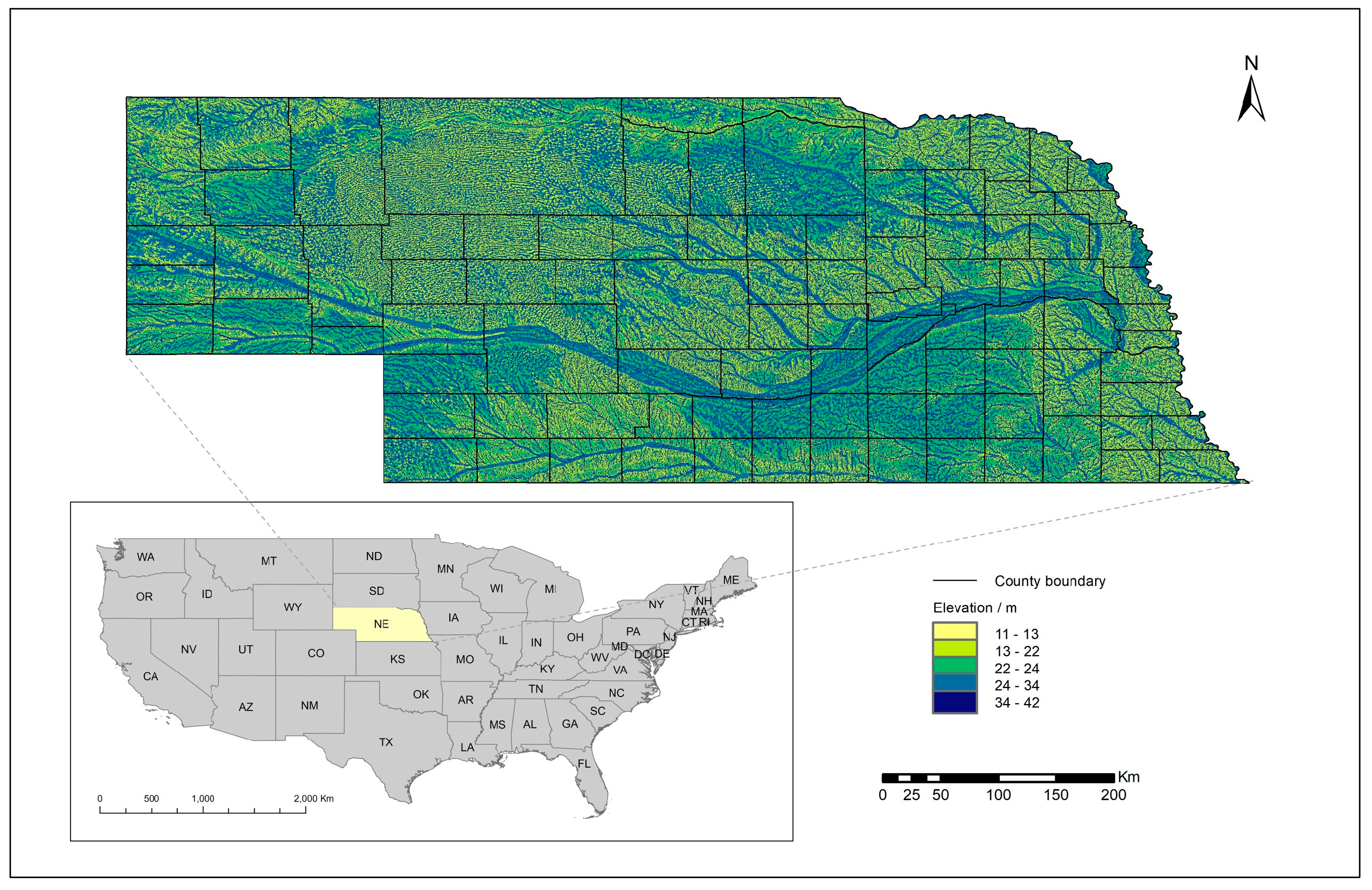
2.1. Study Area

We selected the state of Nebraska, USA, as our study area (Figure 1). Nebraska comprises 93 counties and contributes 75% of the country’s total soybean production [28]. We designed a simulated experiment of soybean area estimation at the county level in this state to evaluate our proposed BAESCM.

2.2. Reference Data

The Cropland Data Layer (CDL) dataset, produced by the U.S. Department of Agriculture (USDA), provides accurate and timely crop maps for the USA [29,30]. Due to the high quality, CDL data were widely used in various pieces of research as reference data or confident training samples [31,32,33]. Similarly, we also used CDL data as ground truth in our study (Figure 2a). The field sampling process is simulated by randomly selecting samples from CDL data. The soybean areas of the 93 counties, calculated through pixel-counting from CDL data, are considered to be the true areas.

2.3. Sentinel-2 Data

Sentinel-2 images (S2 L2A product) acquired from days 200 to 240 of the year 2019 with cloud cover of less than 10% were selected for soybean classification in Nebraska. This period was chosen because remote sensing data in this period were able to capture key features that distinguish soybeans well from other crop types [34]. Specifically, the mean spectral reflectance and the mean NDVI during this period were calculated for soybean classification and clustering in our method. To preserve more spatial and spectral details, all bands were resampled to 10 m resolution.

2.4. Classification Map of Soybean

A classification map is an essential input for area estimation. In this study, we generated two binary classification maps (soybean and non-soybean) through two types of classification methods (classifier-based and index-based methods) based on Sentinel-2 data. For the classifier-based method, we employed the random forest (RF) method as it is one of the most widely used techniques for large-scale crop mapping [35,36,37]. A total of 1000 soybean and 1000 non-soybean samples were randomly selected from CDL to train the RF classifier and generate the soybean map (Figure 2b). Regarding the index-based method, we applied the Greenness and Water Content Composite Index (GWCCI) to map the soybean as it has shown great effectiveness in identifying soybeans in a recent study [34]. GWCCI combines both NDVI and SWIR to enhance the features of soybean:

$$\mathrm{G}\mathrm{W}\mathrm{C}\mathrm{C}\mathrm{I}=\mathrm{N}\mathrm{D}\mathrm{V}\mathrm{I}\times {\mathsf{\rho }}_{\mathrm{S}\mathrm{W}\mathrm{I}\mathrm{R}}$$

(1)

where ${\mathsf{\rho }}_{\mathrm{S}\mathrm{W}\mathrm{I}\mathrm{R}}$ is the reflectance of the SWIR band. The index-based method does not require training samples; instead, a simple threshold was used to identify the soybean pixels (Figure 2c). The threshold was set to 0.17 based on the recommendation from the previous study [34].

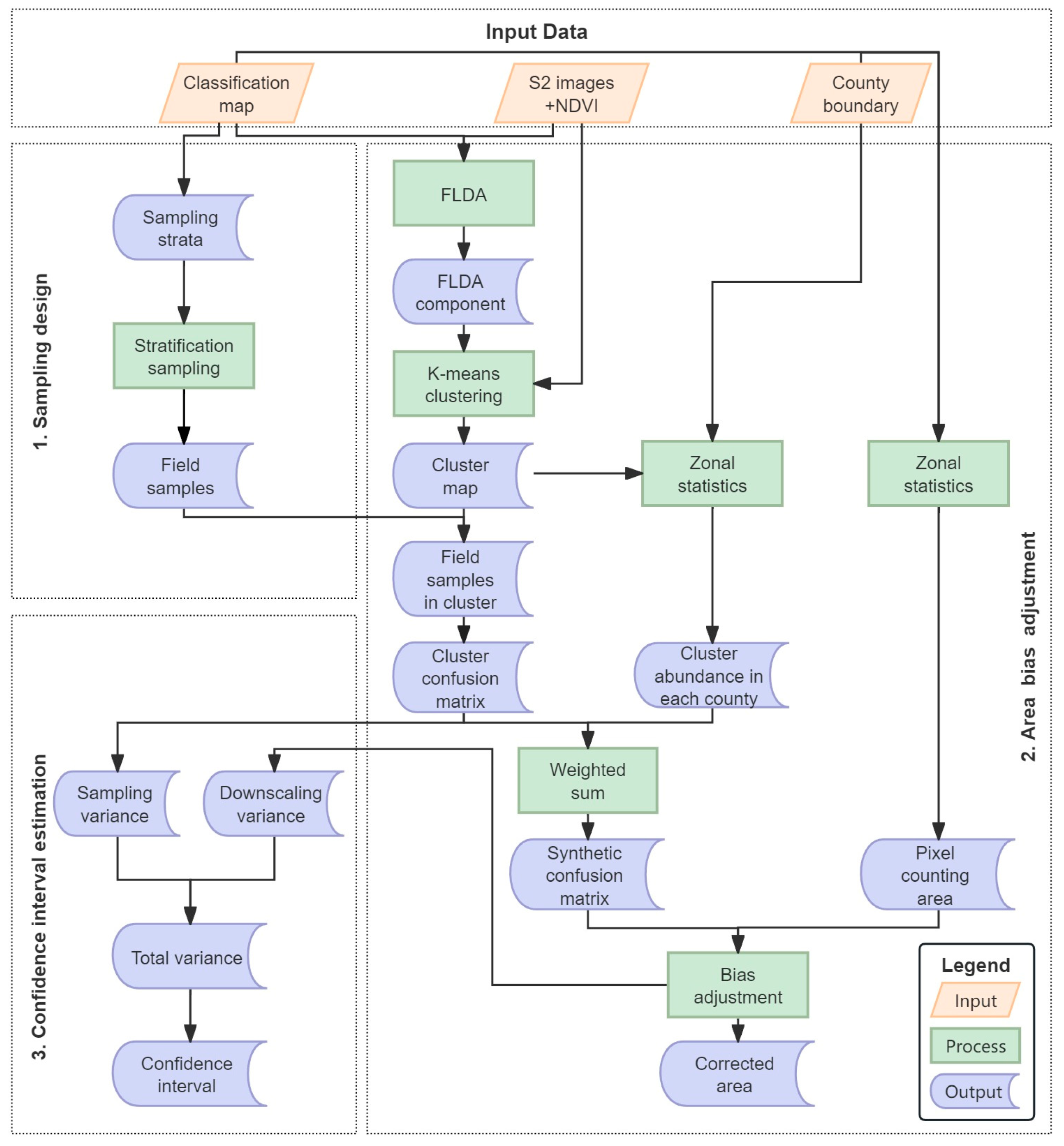
3. Methods

The target of the BAESCM is to estimate the land cover (soybean in this study) area proportion of each subregion (county in the state of Nebraska) based on the classification map and the ground truth samples collected across the global area (the whole state of Nebraska). The BAESCM consists of three major parts (Figure 3): (1) sampling design; (2) area bias adjustment based on synthetic confusion matrix at subregion scale; (3) semi-empirical uncertainty inference for the area estimate.

3.1. Sampling Design

We applied a stratified random sampling strategy to collect ground truth samples across the whole Nebraska state, with the strata defined by the classification map (soybean and non-soybean). Considering convenience in practical field surveys, a disproportionate stratified random sampling was used, with an equal sample number for each stratum. As this is a simulation experiment, the samples were randomly selected from CDL data rather than from actual field investigations. Thus, repeating sampling experiments can be easily conducted. For each classification map (RF or GWCCI), a total of 80 sample sets were simulated, with eight sample sizes varying from 10 to 8000 (i.e., 10, 100, 300, 500, 1000, 2000, 4000, 8000) and ten repetitions for each sample size.

3.2. Area Bias Adjustment Based on Synthetic Confusion Matrix at Subregion Scale

A confusion matrix is the most commonly used tool for evaluating the classification accuracy and describing the classification error distribution. Various area estimators (including the bias-adjusted estimator) can be derived from the confusion matrix as it contains information from both the ground truth samples and the classification map [14]. However, it is impractical to accurately estimate the subregion confusion matrix due to the insufficient samples in each subregion. In the proposed method, we assume that the pixels within a spectral cluster share similar classification error distribution across different subregions, which provides an opportunity to downscale the global classification error information to the subregion scale and support the bias adjustment of the subregion areas.

3.2.1. Spectral Clustering

We applied the K-means method to generate several spectral clusters based on remote sensing data. In addition to the original spectral bands from Sentinel-2 imagery, the Fisher linear discriminative analysis (FLDA) component is also introduced as an input for K-means clustering, as FLDA provides effective features for land cover classification. The training data required in FLDA were selected from the classification map to ensure the independence between the training data and the ground truth samples. For binary classification, FLDA produces only one component. Thus, a total of 12 bands in total (11 original spectral bands and 1 FLDA component) were input for K-means clustering in this study. The number of clusters was empirically set as 6, which is much smaller than the county number 93. As the spectral cluster has similar spectral features, it is reasonable to assume a similar classification error distribution within each cluster. Additionally, the error distributions of different clusters are considered to be independent of each other.

3.2.2. Estimation of Cluster Confusion Matrix

The cluster confusion matrixes were estimated based on the samples belonging to the corresponding cluster. As the number of clusters is much smaller than the number of subregions, the global samples are adequate to support accurate estimation of cluster confusion matrixes. In this study, the ground truth samples were collected with disproportionate stratified random sampling; thus, a stratified estimation formula of the confusion matrix, which is suitable for unequal probability samples, was calculated [16]. Each cell of the confusion matrix (${\mathrm{p}}_{\mathrm{i}\mathrm{j}}^{\left(\mathrm{c}\right)}$ denoting the estimated area proportion with map class $\mathrm{i}$ and reference class $\mathrm{j}$ in cluster $\left(\mathrm{c}\right)$ is calculated as follows:

$${\mathrm{p}}_{\mathrm{i}\mathrm{j}}^{\left(\mathrm{c}\right)}={\mathrm{p}}_{\mathrm{i}+}^{\left(\mathrm{c}\right)}{\displaystyle \frac{{\mathrm{n}}_{\mathrm{i}\mathrm{j}}^{\left(\mathrm{c}\right)}}{{\mathrm{n}}_{\mathrm{i}+}^{\left(\mathrm{c}\right)}}}$$

(2)

where ${\mathrm{p}}_{\mathrm{i}+}^{\left(\mathrm{c}\right)}$ is the proportion of area mapped as class $\mathrm{i}$ in cluster $\mathrm{c}$, ${\mathrm{n}}_{\mathrm{i}\mathrm{j}}^{\left(\mathrm{c}\right)}$ represents the number of samples that fell in the cell with map class $\mathrm{i}$ and reference class $\mathrm{j}$ in cluster $\mathrm{c}$, and ${\mathrm{n}}_{\mathrm{i}+}^{\left(\mathrm{c}\right)}$ represents the marginal totals of samples of map class $\mathrm{i}$ in cluster $\mathrm{c}$.

For binary classification, the cluster confusion matrix of cluster c can be expressed as a Table (

Table 1. Population confusion matrix in term of proportions.

		Reference Class		Total
		1	2
Map class	1	${\mathrm{p}}_{11}^{\left(\mathrm{c}\right)}$	${\mathrm{p}}_{12}^{\left(\mathrm{c}\right)}$	${\mathrm{p}}_{1+}^{\left(\mathrm{c}\right)}$
	2	${\mathrm{p}}_{21}^{\left(\mathrm{c}\right)}$	${\mathrm{p}}_{22}^{\left(\mathrm{c}\right)}$	${\mathrm{p}}_{2+}^{\left(\mathrm{c}\right)}$
	Total	${\mathrm{p}}_{+1}^{\left(\mathrm{c}\right)}$	${\mathrm{p}}_{+2}^{\left(\mathrm{c}\right)}$	1

) or denoted as a matrix (Equation (3)). If very few samples fall into certain clusters (${\mathrm{n}}_{\mathrm{c}}<2$), in some extreme situations (for example, the cluster number is too many and the total samples are small), the corresponding cluster confusion matrix cannot be established. In this case, these clusters with few samples are merged into another cluster with most similar mean spectrum.

$${\mathbf{M}}_{\mathrm{c}}=\left(\begin{array}{cc}{\mathrm{p}}_{11}^{\left(\mathrm{c}\right)}& {\mathrm{p}}_{12}^{\left(\mathrm{c}\right)}\\ {\mathrm{p}}_{21}^{\left(\mathrm{c}\right)}& {\mathrm{p}}_{22}^{\left(\mathrm{c}\right)}\end{array}\right)$$

(3)

3.2.3. Confusion Matrix Synthesis for Subregions

If we assume that the classification error distribution remains consistent from the global scale to the subregion scale for each cluster (${\mathbf{M}}_{\mathrm{c}}\cong {\mathbf{M}}_{\mathrm{c}}^{\left(\mathrm{k}\right)}$), then the confusion matrix of each subregion can be synthetic by the weighted sum of cluster confusion matrix, with the weights of cluster abundance (area proportion) in the subregion:

$${\mathbf{M}}^{\left(\mathrm{k}\right)}=\left(\begin{array}{cc}{\mathrm{p}}_{11}^{\left(\mathrm{k}\right)}& {\mathrm{p}}_{12}^{\left(\mathrm{k}\right)}\\ {\mathrm{p}}_{21}^{\left(\mathrm{k}\right)}& {\mathrm{p}}_{22}^{\left(\mathrm{k}\right)}\end{array}\right)={\sum }_{\mathrm{c}=1}^{\mathrm{m}}{\mathrm{w}}_{\mathrm{c}}^{\left(\mathrm{k}\right)}{\mathbf{M}}_{\mathrm{c}}$$

(4)

where ${\mathbf{M}}^{\left(\mathrm{k}\right)}$ is the synthetic confusion matrix in subregion $\mathrm{k}$, ${\mathrm{w}}_{\mathrm{c}}^{\left(\mathrm{k}\right)}$ is the abundance of cluster $\mathrm{c}$ in subregion k, and m is the cluster number.

3.2.4. Bias Adjustment of Subregion Areas

With the synthetic confusion matrix, the mapped area (derived from pixel-counting) of subregion $\mathrm{k}$ can be corrected by the bias adjustment. With the binary classification case, the corrected area of the target class (${\widehat{\mathrm{p}}}_{+2}^{\left(\mathrm{k}\right)}$, assumed that class 2 is our target class) can be derived as follows:

$$\begin{gathered} {\widehat{\mathrm{p}}}_{+2}^{\left(\mathrm{k}\right)}={\mathrm{p}}_{2+}^{\left(\mathrm{k}\right)}-{\mathrm{d}}_{2+}^{\left(\mathrm{k}\right)}={\mathrm{p}}_{2+}^{\left(\mathrm{k}\right)}-\left({\mathrm{p}}_{21}^{\left(\mathrm{k}\right)}-{\mathrm{p}}_{12}^{\left(\mathrm{k}\right)}\right) \\ ={\mathrm{p}}_{2+}^{\left(\mathrm{k}\right)}-{\sum }_{\mathrm{c}=1}^{\mathrm{m}}{\mathrm{w}}_{\mathrm{c}}^{\left(\mathrm{k}\right)}\left({\mathrm{p}}_{21}^{\left(\mathrm{c}\right)}-{\mathrm{p}}_{12}^{\left(\mathrm{c}\right)}\right) \end{gathered}$$

(5)

where ${\mathrm{p}}_{2+}^{\left(\mathrm{k}\right)}$ are ${\widehat{\mathrm{p}}}_{+2}^{\left(\mathrm{k}\right)}$ are the mapped area and corrected area of the target class in subregion k, and ${\mathrm{d}}_{2+}^{\left(\mathrm{k}\right)}={\sum }_{\mathrm{c}=1}^{\mathrm{m}}{\mathrm{w}}_{\mathrm{c}}^{\left(\mathrm{k}\right)}\left({\mathrm{p}}_{21}^{\left(\mathrm{c}\right)}-{\mathrm{p}}_{12}^{\left(\mathrm{c}\right)}\right)$ is the estimated area bias of subregion k.

3.3. Semi-Empirical Estimation of the Confidence Interval of the Area Estimate

There are two uncertainty sources of the proposed BAESCM: (1) the sampling variance in estimating the cluster confusion matrix, which is induced by the sampling randomness of the ground truth samples; (2) the downscaling variance in the matrix synthetic process, which results from the deviation between the cluster confusion matrixes at the subregion scale and those at the global scale (${\mathbf{M}}_{\mathrm{c}}\ne {\mathbf{M}}_{\mathrm{c}}^{\left(\mathrm{k}\right)}$). Thus, the variance in the estimated subregion area ($\mathrm{V}\mathrm{a}\mathrm{r}\left({\widehat{\mathrm{p}}}_{+2}^{\left(\mathrm{k}\right)}\right)$), which equals to the variance in the estimated area bias ($\mathrm{V}\mathrm{a}\mathrm{r}\left({\mathrm{d}}_{2+}^{\left(\mathrm{k}\right)}\right)$) as the pixel-counting area (${\mathrm{p}}_{2+}^{\left(\mathrm{k}\right)}$) has no variance, consists of two components, sampling variance (${\mathrm{V}\mathrm{a}\mathrm{r}}_{\mathrm{s}\mathrm{a}\mathrm{m}}^{\mathrm{k}}\left({\mathrm{d}}_{2+}^{\left(\mathrm{k}\right)}\right)$) and downscaling variance (${\mathrm{V}\mathrm{a}\mathrm{r}}_{\mathrm{d}\mathrm{o}\mathrm{w}\mathrm{n}\mathrm{s}\mathrm{c}\mathrm{a}\mathrm{l}\mathrm{e}}^{\mathrm{k}}\left({\mathrm{d}}_{2+}^{\left(\mathrm{k}\right)}\right)$).

$$\mathrm{V}\mathrm{a}\mathrm{r}\left({\widehat{\mathrm{p}}}_{+2}^{\left(\mathrm{k}\right)}\right)=\mathrm{V}\mathrm{a}\mathrm{r}\left({\mathrm{d}}_{2+}^{\left(\mathrm{k}\right)}\right)={\mathrm{V}\mathrm{a}\mathrm{r}}_{\mathrm{s}\mathrm{a}\mathrm{m}}^{\left(\mathrm{k}\right)}\left({\mathrm{d}}_{2+}^{\left(\mathrm{k}\right)}\right)+{\mathrm{V}\mathrm{a}\mathrm{r}}_{\mathrm{d}\mathrm{o}\mathrm{w}\mathrm{n}\mathrm{s}\mathrm{c}\mathrm{a}\mathrm{l}\mathrm{e}}^{\left(\mathrm{k}\right)}\left({\mathrm{d}}_{2+}^{\left(\mathrm{k}\right)}\right)$$

(6)

3.3.1. Estimation of the Sampling Variance

The sampling variance for a subregion k is induced by the sampling variance of cluster confusion matrixes; thus it can be expressed as follows:

$$\begin{gathered} {\mathrm{V}\mathrm{a}\mathrm{r}}_{\mathrm{s}\mathrm{a}\mathrm{m}}^{\left(\mathrm{k}\right)}\left({\mathrm{d}}_{2+}^{\left(\mathrm{k}\right)}\right)={\sum }_{\mathrm{c}=1}^{\mathrm{m}}{\left({\mathrm{w}}_{\mathrm{c}}^{\left(\mathrm{k}\right)}\right)}^2{\mathrm{V}\mathrm{a}\mathrm{r}}_{\mathrm{s}\mathrm{a}\mathrm{m}}\left({\mathrm{p}}_{21}^{\left(\mathrm{c}\right)}-{\mathrm{p}}_{12}^{\left(\mathrm{c}\right)}\right) \\ ={\sum }_{\mathrm{c}=1}^{\mathrm{m}}{\left({\mathrm{w}}_{\mathrm{c}}^{\left(\mathrm{k}\right)}\right)}^2{\mathrm{V}\mathrm{a}\mathrm{r}}_{\mathrm{s}\mathrm{a}\mathrm{m}}\left({\widehat{\mathrm{p}}}_{+2}^{\left(\mathrm{c}\right)}\right) \end{gathered}$$

(7)

where ${\mathrm{w}}_{\mathrm{c}}^{\left(\mathrm{k}\right)}$ is the abundance of cluster $\mathrm{c}$ in subregion $\mathrm{k}$ and ${\mathrm{V}\mathrm{a}\mathrm{r}}_{\mathrm{s}\mathrm{a}\mathrm{m}}\left({\widehat{\mathrm{p}}}_{+2}^{\left(\mathrm{c}\right)}\right)$ is the sampling variance of the target area estimate of cluster $\mathrm{c}$.

In each stratum, the samples included in each cluster can be regarded as simple random samples. This is because the designed stratified sampling is conducted at the global scale and the clustering process is independent from the sampling process. Thus, ${\mathrm{V}\mathrm{a}\mathrm{r}}_{\mathrm{s}\mathrm{a}\mathrm{m}}\left({\widehat{\mathrm{p}}}_{+2}^{\left(\mathrm{c}\right)}\right)$ can be estimated by the poststratified estimator [14]:

$$\begin{gathered} {\mathrm{V}\mathrm{a}\mathrm{r}}_{\mathrm{s}\mathrm{a}\mathrm{m}}\left({\widehat{\mathrm{p}}}_{+2}^{\left(\mathrm{c}\right)}\right)={\displaystyle \frac{1}{{\mathrm{n}}_{\mathrm{c}}}}{\sum }_{\mathrm{t}=1}^2{\mathrm{p}}_{\mathrm{t}+}^{\left(\mathrm{c}\right)}{{(\mathrm{S}}_{\mathrm{t}}^{\left(\mathrm{c}\right)})}^2+{\displaystyle \frac{1}{{{\mathrm{n}}_{\mathrm{c}}}^2}}{\sum }_{\mathrm{t}=1}^2\left(1-{\mathrm{p}}_{\mathrm{t}+}^{\left(\mathrm{c}\right)}\right){{(\mathrm{S}}_{\mathrm{t}}^{\left(\mathrm{c}\right)})}^2 \\ \mathrm{w}\mathrm{h}\mathrm{e}\mathrm{r}\mathrm{e} {{(\mathrm{S}}_{\mathrm{t}}^{\left(\mathrm{c}\right)})}^2={\displaystyle \frac{{\mathrm{p}}_{\mathrm{t}2}^{\left(\mathrm{c}\right)}}{{\mathrm{p}}_{\mathrm{t}+}^{\left(\mathrm{c}\right)}}}(1-{\displaystyle \frac{{\mathrm{p}}_{\mathrm{t}2}^{\left(\mathrm{c}\right)}}{{\mathrm{p}}_{\mathrm{t}+}^{\left(\mathrm{c}\right)}}})\times {\displaystyle \frac{{\mathrm{n}}_{\mathrm{t}}^{\left(\mathrm{c}\right)}}{{\mathrm{n}}_{\mathrm{t}}^{\left(\mathrm{c}\right)}-1}} \end{gathered}$$

(8)

here, ${\mathrm{n}}_{\mathrm{c}}$ and ${\mathrm{n}}_{\mathrm{t}}^{\left(\mathrm{c}\right)}$ are the total sample number in cluster $\mathrm{c}$ and the number of samples belonging to mapping class $\mathrm{t}$ in cluster $\mathrm{c}$; ${\displaystyle \frac{{\mathrm{p}}_{\mathrm{t}2}^{\left(\mathrm{c}\right)}}{{\mathrm{p}}_{\mathrm{t}+}^{\left(\mathrm{c}\right)}}}$ is the abundance of true target class (2) in the samples belonging to mapping class $\mathrm{t}$ (t = 1 or 2) in cluster $\mathrm{c}$; ${{(\mathrm{S}}_{\mathrm{t}}^{\left(\mathrm{c}\right)})}^2$ is the estimated variance of stratum of mapping class $\mathrm{t}$ in cluster $\mathrm{c}$; ${\displaystyle \frac{{\mathrm{n}}_{\mathrm{t}}^{\left(\mathrm{c}\right)}}{{\mathrm{n}}_{\mathrm{t}}^{\left(\mathrm{c}\right)}-1}}$ is the adjustment factor for small sample size. The poststratified estimator requires adequate samples in each stratum (mapping class 1 and 2) for a cluster. If there are few samples (<2) in any stratum, the ${\mathrm{V}\mathrm{a}\mathrm{r}}_{\mathrm{s}\mathrm{a}\mathrm{m}}\left({\widehat{\mathrm{p}}}_{+2}^{\left(\mathrm{k}\right)}\right)$ should be estimated based on the direct estimator:

$${\mathrm{V}\mathrm{a}\mathrm{r}}_{\mathrm{s}\mathrm{a}\mathrm{m}}\left({\widehat{\mathrm{p}}}_{+2}^{\left(\mathrm{k}\right)}\right)={\displaystyle \frac{{\mathrm{p}}_{+2}^{\left(\mathrm{c}\right)}(1-{\mathrm{p}}_{+2}^{\left(\mathrm{c}\right)})}{{\mathrm{n}}_{\mathrm{c}}}}\times {\displaystyle \frac{{\mathrm{n}}_{\mathrm{c}}}{{\mathrm{n}}_{\mathrm{c}}-1}}$$

(9)

3.3.2. Estimation of the Downscaling Variance

BAESCM assumes that the classification error distribution remains consistent from the global scale to the subregion scale. However, it could vary across different subregions in reality, leading to the downscaling variance in the synthetic process. Unfortunately, there is no statistically rigorous method to estimate the downscaling variance. In this study, we proposed a semi-empirical estimate for this term. We observe that the estimated bias by BAESCM might be not very accurate; however, the direction of the estimated bias (positive or negative) is confidentially correct (supposed 99% probability of being correct). This means that the half confidence interval of ${\mathrm{d}}_{2+}^{\mathrm{k}}$ at the 0.01 level should not be larger than ${\mathrm{d}}_{2+}^{\mathrm{k}}$ itself. Thus, the downscaling variance can be expressed as follows:

$${\mathrm{V}\mathrm{a}\mathrm{r}}_{\mathrm{d}\mathrm{o}\mathrm{w}\mathrm{n}\mathrm{s}\mathrm{c}\mathrm{a}\mathrm{l}\mathrm{e}}^{\left(\mathrm{k}\right)}\left({\mathrm{d}}_{2+}^{\left(\mathrm{k}\right)}\right)={\left({\displaystyle \frac{1}{{\mathrm{z}}_{1-\frac{\mathsf{\alpha }}{2}}}}\left|{\mathrm{d}}_{2+}^{\left(\mathrm{k}\right)}\right|\right)}^2$$

(10)

where ${\mathrm{z}}_{1-{\displaystyle \frac{\mathsf{\alpha }}{2}}}$ denote the two tailed test z-score at $\mathsf{\alpha }$ levels ($\mathsf{\alpha }=$0.01). Equation (10) means a conversion from empirical interval to downscaling variance. The downscaling variance is not related to the sample size and, thus, cannot be diminished by increasing the sample size.

3.3.3. Estimation of Confidence Interval of BAESCM Area Estimate

With the estimated sampling variance and downscaling variance, the confidence interval at $\mathsf{\alpha }$ level for the area estimate in subregion $\mathrm{k}$ can be derived as follows:

$${\widehat{\mathrm{p}}}_{+2}^{\mathrm{k}}\pm {\mathrm{z}}_{1-{\displaystyle \frac{\mathsf{\alpha }}{2}}}\sqrt{{\mathrm{V}\mathrm{a}\mathrm{r}}_{\mathrm{s}\mathrm{a}\mathrm{m}}^{\left(\mathrm{k}\right)}\left({\mathrm{d}}_{2+}^{\left(\mathrm{k}\right)}\right)+{\mathrm{V}\mathrm{a}\mathrm{r}}_{\mathrm{d}\mathrm{o}\mathrm{w}\mathrm{n}\mathrm{s}\mathrm{c}\mathrm{a}\mathrm{l}\mathrm{e}}^{\left(\mathrm{k}\right)}\left({\mathrm{d}}_{2+}^{\left(\mathrm{k}\right)}\right)}$$

(11)

4. Results

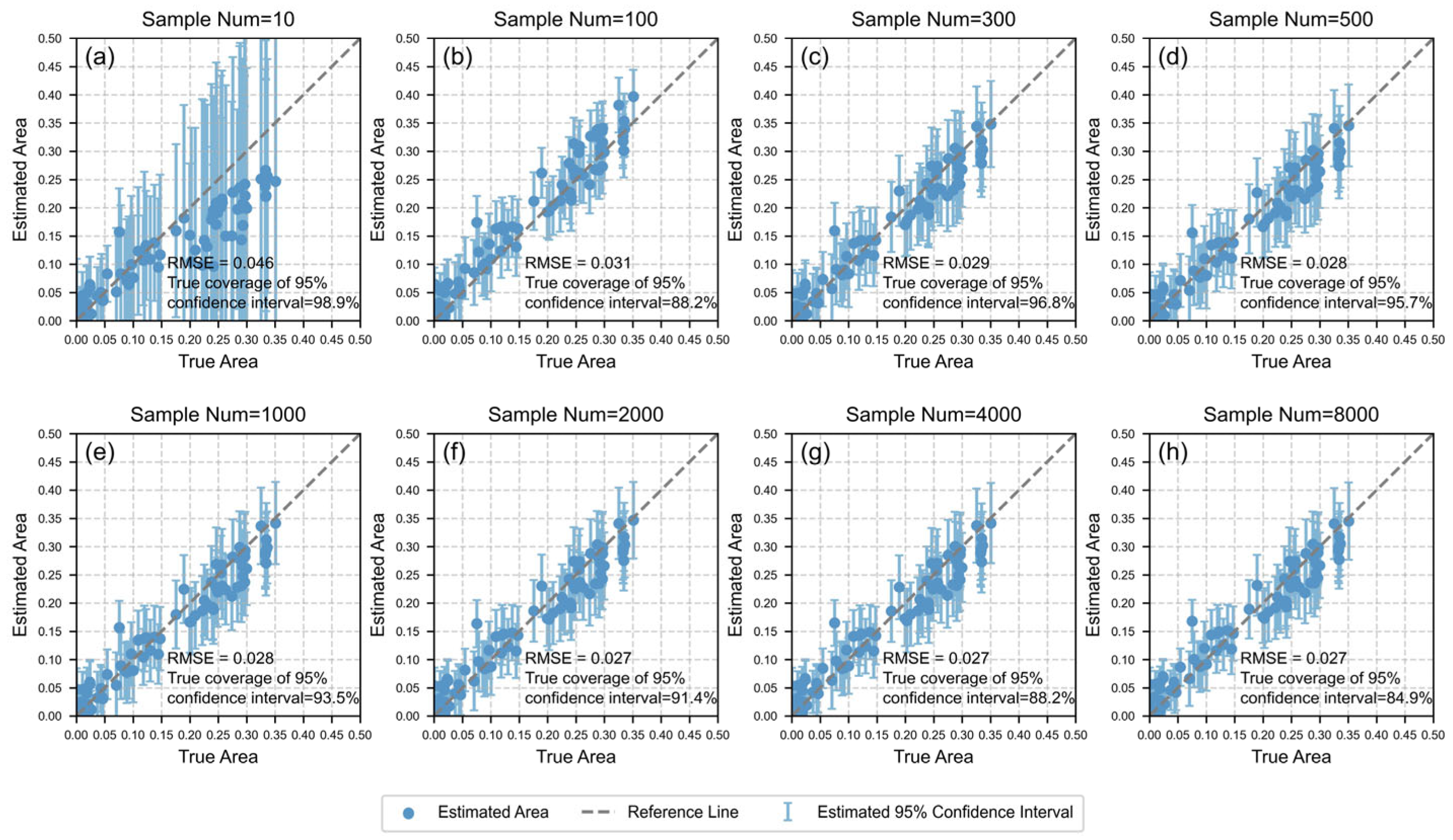
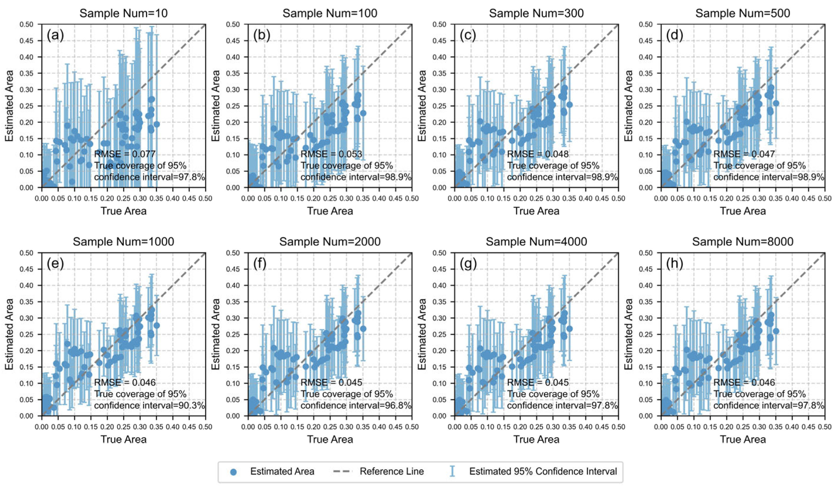
4.1. Area Estimation Results by BAESCM

The soybean areas of 93 counties in Nebraska state, along with their corresponding confidence intervals, were estimated using the proposed BAESCM. Across varying sample sizes, BAESCM consistently provided more accurate area estimates than the pixel-counting method. As shown in Figure 4, the pixel-counting areas from both the RF and GWCCI classification maps showed significant overestimations compared to the true areas, with RMSEs of 0.058 and 0.125, respectively. In contrast, the areas corrected using the BAESCM method were closer to the true areas, with RMSEs ranging from 0.027 to 0.046 for the RF map (Figure 5a–h) and from 0.045 to 0.077 for the GWCCI map (Figure 6a–h). In general, the RMSE of BAESCM is reduced by 21–64% compared to pixel-counting method. Even in the extreme case of 10 samples, BAESCM outperformed pixel-counting in terms of accuracy. As the sample size increased, the RMSE of BAESCM slightly decreased due to reduced sampling variance. However, the RMSE remains stable when the sample size reaches a certain level. Additionally, the predicted 95% confidence intervals included the true areas for 85~99% of the counties, regardless of the sample size and classification map used (RF or GWCCI). These results demonstrate that the proposed method effectively corrects the area bias of classification maps and provides a relatively reliable estimate of the associated uncertainty, even with limited sample sizes.

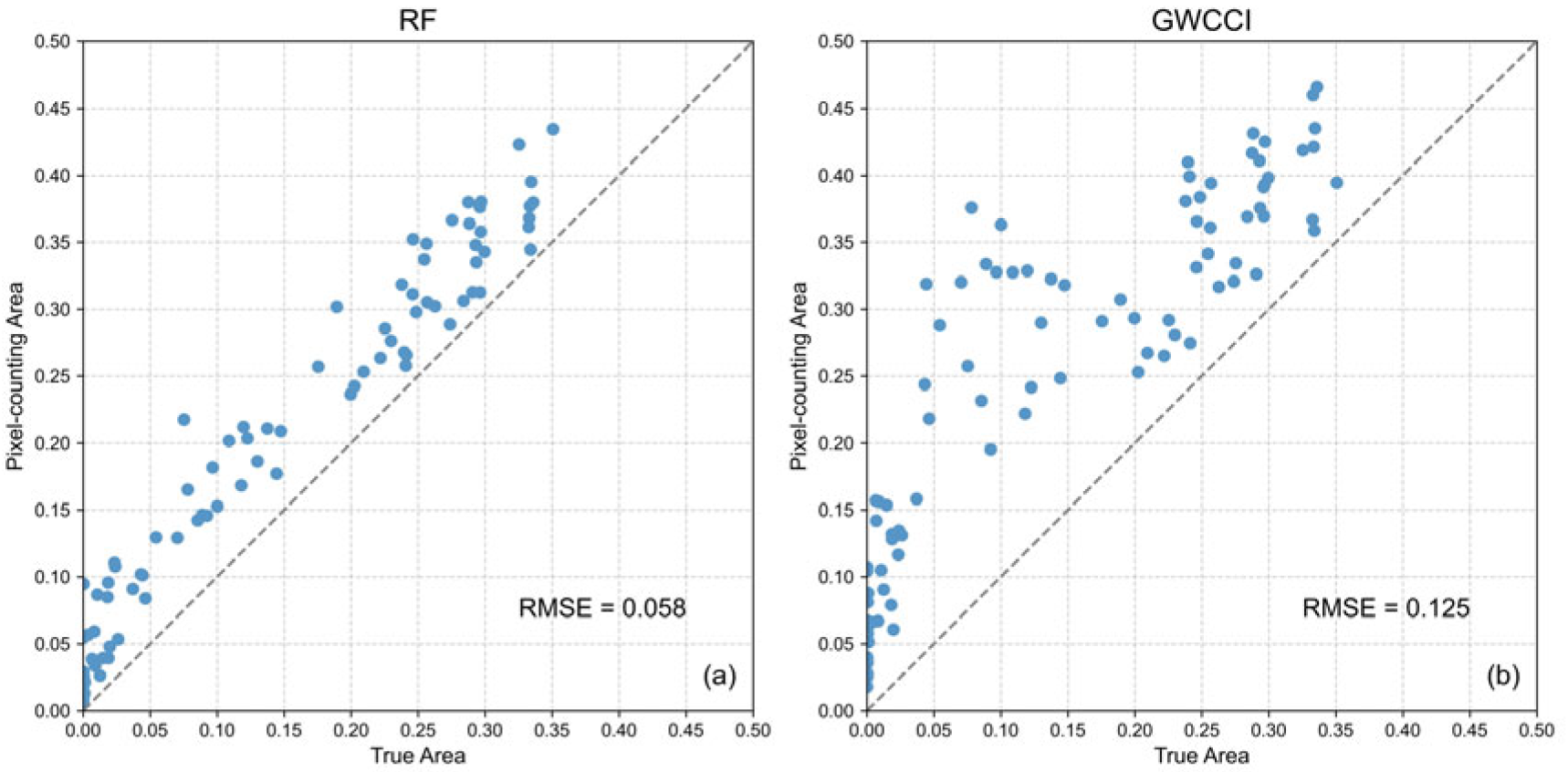
4.2. Comparison with Traditional Design-Based Methods

We further compared the proposed BAESCM with the stratified estimator, a widely recommended design-based method [14]. The total sample sizes for BAESCM range from 10 to 8000. As the stratified estimator requires samples from each subregion, we varied the sample sizes from 2 to 90 per county, corresponding to a total sample size ranging from 186 to 8370 for the design-based method. As shown in Figure 7, BAESCM outperforms the stratified estimator when the total sample size is small. For example, with a total sample size of 500, BAESCM achieves area accuracies (RMSEs) of 0.028 and 0.047 for the RF and GWCCI maps, respectively. In contrast, the stratified estimator requires approximately 6000 samples for the RF map and 1800 samples for the GWCCI map to achieve similar accuracy. However, when the total sample size is large (approximately over 7000 for the RF map and 3000 for the GWCCI map), the stratified estimator becomes the better choice, as it is an unbiased estimator, and its accuracy improves indefinitely with increasing sample size. Thus, BAESCM is the better option when the sample size is limited, whereas the traditional stratified estimator is recommended when a sufficiently large sample size is available.

5. Discussions

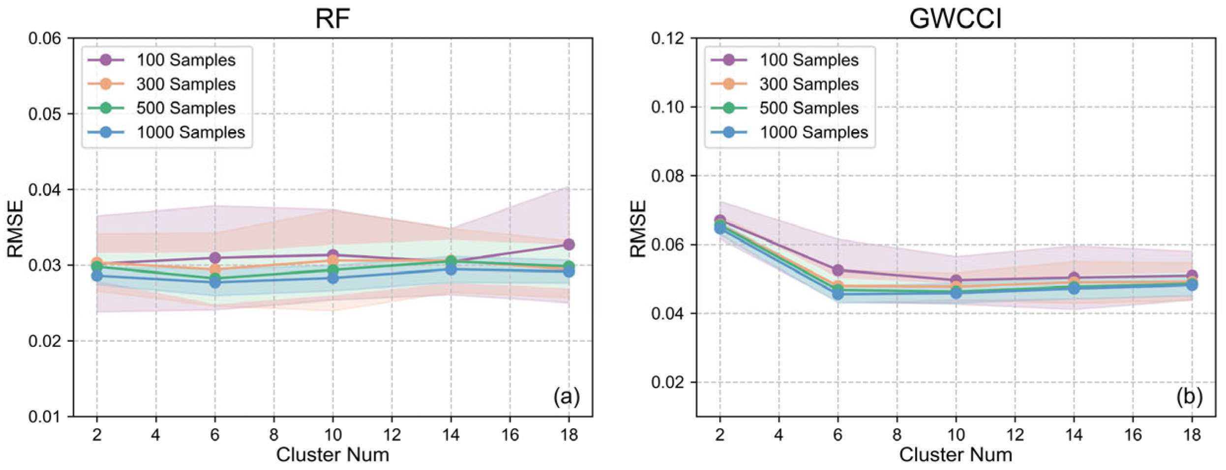
5.1. Selection of Cluster Number for the BAESCM Method

The cluster number is an empirical parameter in our method. Reducing the cluster number decreases the sampling variance because the sample size within each cluster increases; however, this also leads to increased downscaling variance because the classification error distribution is more diverse within a larger cluster. Conversely, increasing the cluster number reduces the heterogeneity of classification error distribution within clusters but increases the sampling variance increases. Therefore, the selection of the number of clusters is closely related to the sample size and the intra-cluster heterogeneity of classification error.

We, thus, further examine how the performance of BAESCM varies with different cluster numbers under different sample sizes (Figure 8). For the RF classification map, the optimal cluster number is 2 when the sample size is 100 and increases to 6 when the sample size achieves 300 or higher. However, the cluster number is not a very sensitive parameter for an RF classification map. Even two clusters are adequate for the BAESCM method, probably because the classification error distribution of RF is relatively homogenous. For the GWCCI classification map, cluster number is not a very sensitive parameter either, except that the RMSE increases greatly when the cluster number is 2. This indicates that the setting of cluster numbers is not very difficult in most cases.

5.2. Advantages and Limitations

Our proposed BAESCM method achieved the expected performance in subregion area estimation, as demonstrated by the simulated experiments. It requires fewer samples to estimate the area of subregions compared with traditional design-based estimators and, thus, is more recommended in the case of a limited sample size. Additionally, it has more generalizable and simpler assumptions and lower computational complexity; thus, it has a wider application scope. Due to the high cost of sample acquisition and the difficulty in establishing a reasonable model, both the traditional design-based and model-based methods are not suitable for subregion area estimations in real scenarios. Therefore, BAESCM provides a unique method for effective subregion area estimation in real applications.

However, some limitations remain in our approach. Firstly, BAESCM is a biased estimator, of which the estimation error cannot be reduced infinitely with the increasing sample size. This indicates that BAESCM outperforms traditional design-based methods only in the case of a small sample size. If the sample size is adequately large, the unbiased design-based method is still a better choice. Moreover, as the downscaling variance (uncertainty of bias) increases, the sample size threshold at which traditional design-based methods outperform BAESCM decreases, thereby narrowing the range of sample sizes for which BAESCM is advantageous. Secondly, the confidence interval is predicted by a semi-empirical method, where the downscaling variance is not estimated rigorously. Thus, further improvement in estimating downscaling variance should be required in the future, which not only benefits the confident interval inference but also helps predict the range of sample sizes within which the BAESCM method outperforms the original design-based methods. Thirdly, we empirically selected the K-means method with spectral bands and FLDA as feature input to generate the clusters in the proposed method. However, there might be better clustering strategies that are able to generate clusters with more consistent classification error distribution within each cluster and, thus, improve the subregional area estimation results. As the factors affecting classification error distribution are complex, further research is required in order to select a better clustering strategy.

6. Conclusions

In this study, we proposed the BAESCM method for estimating land cover areas in multiple subregions, where sufficient ground truth samples are often unavailable. The core idea of BAESCM is to introduce a synthetic confusion matrix for each subregion, which downscales the global sample information to the subregion scale, thereby effectively correcting the area bias in the classification map. Moreover, we proposed a semi-empirical method to estimate the uncertainty of the corrected areas, offering more valuable estimating result for users. The simulated experiments confirm the superiority of the proposed BAESCM over the traditional stratified estimator, particularly in cases with limited sample size. In summary, BAESCM provides a unique and practical method for effective subregion area estimation in real-world scenarios where ground truth samples are often limited.

References

- Gallego, F.J. Remote Sensing and Land Cover Area Estimation. Int. J. Remote Sens. 2004, 25, 3019–3047. [Google Scholar] [CrossRef]
- Pradhan, S. Crop Area Estimation Using GIS, Remote Sensing and Area Frame Sampling. Int. J. Appl. Earth Obs. Geoinf. 2001, 3, 86–92. [Google Scholar] [CrossRef]
- Bégué, A.; Arvor, D.; Bellon, B.; Betbeder, J.; De Abelleyra, D.; Ferraz, R.P.D.; Lebourgeois, V.; Lelong, C.; Simões, M.; Verón, S.R. Remote Sensing and Cropping Practices: A Review. Remote Sens. 2018, 10, 99. [Google Scholar] [CrossRef]
- Weiss, M.; Jacob, F.; Duveiller, G. Remote Sensing for Agricultural Applications: A Meta-Review. Remote Sens. Environ. 2020, 236, 111402. [Google Scholar] [CrossRef]
- Liu, J.; Wang, L.; Yang, F.; Yang, L.; Wang, X. Remote Sensing Estimation of Crop Planting Area Based on HJ Time-Series Images. Trans. Chin. Soc. Agric. Eng. 2015, 31, 199–206. [Google Scholar]
- Czaplewski, R.L.; Catts, G.P. Calibration of Remotely Sensed Proportion or Area Estimates for Misclassification Error. Remote Sens. Environ. 1992, 39, 29–43. [Google Scholar] [CrossRef]
- Ozdogan, M.; Woodcock, C.E. Resolution Dependent Errors in Remote Sensing of Cultivated Areas. Remote Sens. Environ. 2006, 103, 203–217. [Google Scholar] [CrossRef]
- Richards, J. Classifier Performance and Map Accuracy. Remote Sens. Environ. 1996, 57, 161–166. [Google Scholar] [CrossRef]
- Stehman, S. Comparing Estimators of Gross Change Derived from Complete Coverage Mapping Versus Statistical Sampling of Remotely Sensed Data. Remote Sens. Environ. 2005, 96, 466–474. [Google Scholar] [CrossRef]
- McRoberts, R.E. Satellite Image-Based Maps: Scientific Inference or Pretty Pictures? Remote Sens. Environ. 2011, 115, 715–724. [Google Scholar] [CrossRef]
- Li, Y.; Zhu, X.; Pan, Y.; Gu, J.; Zhao, A.; Liu, X. A Comparison of Model-Assisted Estimators to Infer Land Cover/Use Class Area Using Satellite Imagery. Remote Sens. 2014, 6, 8904–8922. [Google Scholar] [CrossRef]
- McRoberts, R.E. Probability- and Model-Based Approaches to Inference for Proportion Forest Using Satellite Imagery as Ancillary Data. Remote Sens. Environ. 2010, 114, 1017–1025. [Google Scholar] [CrossRef]
- Ståhl, G.; Saarela, S.; Schnell, S.; Holm, S.; Breidenbach, J.; Healey, S.P.; Patterson, P.L.; Magnussen, S.; Næsset, E.; McRoberts, R.E.; et al. Use of Models in Large-Area Forest Surveys: Comparing Model-Assisted, Model-Based and Hybrid Estimation. For. Ecosyst. 2016, 3, 5. [Google Scholar] [CrossRef]
- Stehman, S.V. Estimating Area from an Accuracy Assessment Error Matrix. Remote Sens. Environ. 2013, 132, 202–211. [Google Scholar] [CrossRef]
- Stehman, S.V. Model-Assisted Estimation as a Unifying Framework for Estimating the Area of Land Cover and Land-Cover Change from Remote Sensing. Remote Sens. Environ. 2009, 113, 2455–2462. [Google Scholar] [CrossRef]
- Stehman, S.V.; Foody, G.M. Key Issues in Rigorous Accuracy Assessment of Land Cover Products. Remote Sens. Environ. 2019, 231, 111199. [Google Scholar] [CrossRef]
- Hansen, M.H.; Madow, W.G.; Tepping, B.J. An Evaluation of Model-Dependent and Probability-Sampling Inferences in Sample Surveys. J. Am. Stat. Assoc. 1983, 78, 776–793. [Google Scholar] [CrossRef]
- McRoberts, R.E.; Walters, B.F. Statistical Inference for Remote Sensing-Based Estimates of Net Deforestation. Remote Sens. Environ. 2012, 124, 394–401. [Google Scholar] [CrossRef]
- Breidenbach, J.; McRoberts, R.E.; Astrup, R. Empirical Coverage of Model-Based Variance Estimators for Remote Sensing Assisted Estimation of Stand-Level Timber Volume. Remote Sens. Environ. 2016, 173, 274–281. [Google Scholar] [CrossRef]
- Broich, M.; Stehman, S.V.; Hansen, M.C.; Potapov, P.; Shimabukuro, Y.E. A Comparison of Sampling Designs for Estimating Deforestation from Landsat Imagery: A Case Study of the Brazilian Legal Amazon. Remote Sens. Environ. 2009, 113, 2448–2454. [Google Scholar] [CrossRef]
- Kleinewillinghöfer, L.; Olofsson, P.; Pebesma, E.; Meyer, H.; Buck, O.; Haub, C.; Eiselt, B. Unbiased Area Estimation Using Copernicus High Resolution Layers and Reference Data. Remote Sens. 2022, 14, 4903. [Google Scholar] [CrossRef]
- McRoberts, R.E.; Liknes, G.C.; Domke, G.M. Using a Remote Sensing-Based, Percent Tree Cover Map to Enhance Forest Inventory Estimation. For. Ecol. Manag. 2014, 331, 12–18. [Google Scholar] [CrossRef]
- Dong, Q.; Chen, X.; Chen, J.; Yin, D.; Zhang, C.; Xu, F.; Rao, Y.; Shen, M.; Chen, Y.; Stein, A. Bias of Area Counted from Sub-Pixel Map: Origin and Correction. Sci. Remote Sens. 2022, 6, 100069. [Google Scholar] [CrossRef]
- McRoberts, R.E. A Model-Based Approach to Estimating Forest Area. Remote Sens. Environ. 2006, 103, 56–66. [Google Scholar] [CrossRef]
- Ståhl, G.; Holm, S.; Gregoire, T.G.; Gobakken, T.; Næsset, E.; Nelson, R. Model-Based Inference for Biomass Estimation in a LiDAR Sample Survey in Hedmark County, NorwayThis Article Is One of a Selection of Papers from Extending Forest Inventory and Monitoring over Space and Time. Can. J. For. Res. 2011, 41, 96–107. [Google Scholar] [CrossRef]
- Chen, Q.; McRoberts, R.E.; Wang, C.; Radtke, P.J. Forest Aboveground Biomass Mapping and Estimation Across Multiple Spatial Scales Using Model-Based Inference. Remote Sens. Environ. 2016, 184, 350–360. [Google Scholar] [CrossRef]
- Lohr, S.L. Sampling: Design and Analysis; Chapman and Hall/CRC: London, UK, 2021. [Google Scholar]
- Johnson, D.M. An Assessment of Pre- and within-Season Remotely Sensed Variables for Forecasting Corn and Soybean Yields in the United States. Remote Sens. Environ. 2014, 141, 116–128. [Google Scholar] [CrossRef]
- Boryan, C.; Yang, Z.; Mueller, R.; Craig, M. Monitoring US Agriculture: The US Department of Agriculture, National Agricultural Statistics Service, Cropland Data Layer Program. Geocarto Int. 2011, 26, 341–358. [Google Scholar] [CrossRef]
- Lark, T.J.; Mueller, R.M.; Johnson, D.M.; Gibbs, H.K. Measuring Land-Use and Land-Cover Change Using the U.S. Department of Agriculture’s Cropland Data Layer: Cautions and Recommendations. Int. J. Appl. Earth Obs. Geoinf. 2017, 62, 224–235. [Google Scholar] [CrossRef]
- Hao, P.; Di, L.; Zhang, C.; Guo, L. Transfer Learning for Crop Classification with Cropland Data Layer Data (CDL) as Training Samples. Sci. Total Environ. 2020, 733, 138869. [Google Scholar] [CrossRef]
- Sun, Z.; Di, L.; Fang, H. Using Long Short-Term Memory Recurrent Neural Network in Land Cover Classification on Landsat and Cropland Data Layer Time Series. Int. J. Remote Sens. 2019, 40, 593–614. [Google Scholar] [CrossRef]
- Zhang, C.; Di, L.; Hao, P.; Yang, Z.; Lin, L.; Zhao, H.; Guo, L. Rapid In-Season Mapping of Corn and Soybeans Using Machine-Learned Trusted Pixels from Cropland Data Layer. Int. J. Appl. Earth Obs. Geoinf. 2021, 102, 102374. [Google Scholar] [CrossRef]
- Chen, H.; Li, H.; Liu, Z.; Zhang, C.; Zhang, S.; Atkinson, P.M. A Novel Greenness and Water Content Composite Index (GWCCI) for Soybean Mapping from Single Remotely Sensed Multispectral Images. Remote Sens. Environ. 2023, 295, 113679. [Google Scholar] [CrossRef]
- Belgiu, M.; Drăguţ, L. Random Forest in Remote Sensing: A Review of Applications and Future Directions. ISPRS J. Photogramm. Remote Sens. 2016, 114, 24–31. [Google Scholar] [CrossRef]
- Breiman, L. Random Forests. Mach. Learn. 2001, 45, 5–32. [Google Scholar] [CrossRef]
- Haas, J.; Ban, Y. Urban Growth and Environmental Impacts in Jing-Jin-Ji, the Yangtze, River Delta and the Pearl River Delta. Int. J. Appl. Earth Obs. Geoinf. 2014, 30, 42–55. [Google Scholar] [CrossRef]