Geospatial Robust Wheat Yield Prediction Using Machine Learning and Integrated Crop Growth Model and Time-Series Satellite Data

Abstract

Accurate crop yield modeling (CYM) is inherently challenging due to the complex, nonlinear, and temporally dynamic interactions of biotic and abiotic factors. Crop traits, which historically capture the cumulative effect of these factors, exhibit functional relationships critical for optimizing productivity. This underscores the necessity of multi-trait-based CYM approaches. Crop growth models enable trait dynamics with reflectance data and spectral indices as proxies for crop health and traits, respectively, to have real-time, spatially explicit monitoring. The Agricultural Production Systems sIMulator was calibrated to simulate multiple traits across the growth season based on geo-tagged wheat field ground information. Reflectance and spectral indices were processed for the geo-tagged fields across temporal observations to enable real-time, spatially explicit monitoring. Based on these parameters, this study addresses a critical gap in existing CYM frameworks by proposing a machine learning-based model that synergized multiple crop traits with reflectance and spectral indices to generate site-specific yield estimates. The performance evaluation revealed that the Long Short-Term Memory (LSTM) model achieved superior accuracy for the integrated parameters (RMSE = 250.68 kg/ha, MAE = 193.76 kg/ha, and R² = 0.84), followed by traits alone. The Random Forest model followed the LSTM model, with an RMSE = 293.56 kg/ha, MAE = 230.68 kg/ha, and R² = 0.78 for integrated parameters, and an RMSE = 291.73 kg/ha, MAE = 223.17 kg/ha, and R² = 0.78 for crop traits. The superior prediction demonstrated the dominant role of multiple crop traits with satellite-derived reflectance metrics to develop robust CYM frameworks capable of capturing intra- and inter-field yield variability.

1. Introduction

Crop yield is governed by complex, nonlinear interactions of a diverse range of biotic and abiotic factors, such as genetics, climate variability, and agricultural management practices [1], that collectively determine yield outcomes [2]. These interactions exhibit temporal sensitivity and spatial heterogeneity, posing significant challenges for accurate crop yield modeling (CYM) [3]. The complexity is further complimented by numerous interdependent factors influenced by external conditions, often with rigid constraints [4]. This modeling complexity resulted in a wide range of crop yield models, including statistical [5], mathematical [6], mechanistic [7], radiative [8], and computer vision-based approaches [9], employed worldwide and across different crops. Each prediction model has inherent advantages and limitations [10]. For example, satellite data enable spatiotemporal monitoring with the limitation of image quality dependency on cloud cover and atmospheric conditions. Similarly, process-based crop growth models (CGMs), while elucidating biological mechanisms, demand extensive ground data on varietal characteristics, soil variation, and management practices. Additionally, these models are unable to predict spatiotemporal variations over large areas without remote sensing data in addition to being resource intensive and time consuming [11]. Despite advancements, no universally accepted method exists, necessitating synergistic approaches that leverage complementary technologies and critical factors to offer robustness and reliability for crop yield prediction [10].

Photosynthesis and crop traits are interconnected and depend on farm management practices and climatic conditions. These traits determine light interception and energy conversion during photosynthesis, while photosynthetic efficiency regulates trait development, collectively shaping crop productivity [12,13]. The LAI, a structural trait crucial to crop photosynthesis, biomass accumulation, and growth dynamics, serves as a robust proxy for yield prediction [14,15,16]. Spatial variability in the LAI correlates with soil properties (e.g., soil moisture and nitrogen content), canopy architecture, and evapotranspiration rates, making it inextricably connected with crop yield [17]. The integration of the LAI into models like the Simple Algorithm for Yield (SAFY) has improved yield estimation accuracy [18], yet plant phenotyping platforms remain constrained by insufficient tools for high-throughput trait measurement, limiting breeders’ capacity to optimize yield strategies [19].

Chlorophyll content, a biochemical proxy for plant health and nitrogen status, enhances yield prediction by differentiating stress responses in areas with similar LAIs [20,21]. For instance, a study demonstrated that chlorophyll measurements distinguish subtle agronomic variations in small plots, enabling precision farming applications [20]. Similarly, the evaluation of five winter wheat cultivars further revealed that the LAI and chlorophyll content, significantly influenced by genotype, nutrient availability, and seasonal fluctuations, jointly predict yield potential. Increased yield is associated with a high chlorophyll content and LAI but was notably affected by post-flowering chlorophyll decline, emphasizing the necessity to monitor both traits during key phenological stages, particularly during flowering to early grain filling, for accurate prediction [22].

The leaf dry matter content (Cm) quantifies the capacity of a plant to convert absorbed radiation into biomass, reflecting structural and biochemical leaf properties. These properties depend on the specific leaf area (LSA, the inverse of the leaf mass per unit area) and leaf nitrogen content (LNC), which governs chlorophyll a b (Cab) synthesis [23,24,25]. Similarly, the relative water content (Cw) functions as a critical indicator of plant stress responses, particularly under disease or drought conditions, as demonstrated in studies linking Cw to physiological resilience [16,26]. To comprehensively capture field-scale variability, yield prediction models must integrate these multi-trait parameters, moving beyond the conventional reliance on the LAI. While the LAI remains widely adopted due to its direct linkage to photosynthesis and biomass [27], many crop growth models face limitations in simulating additional traits. This constraint can be overcome by transformation formulas [25] or advanced CGMs capable of multiple-trait simulation and integration.

Among CGMs, the Agricultural Production Systems sIMulator (APSIM) model has the ability to dynamically simulate multiple crop traits using transformational formulas [25]. The APSIM uses atmospheric conditions, soil properties, and crop ecological processes, enabling robust evaluations of crop growth under diverse management practices [28]. A comparative study of the Decision Support System for Agrotechnology Transfer (DSSAT) and APSIM across 155 Pakistani wheat fields in Faisalabad demonstrated their utility as decision-support tools [29]. The DSSAT achieved higher accuracy for yield prediction, while the APSIM excelled in phenology and biomass simulations. These findings underscore the complementary strengths of process-based models in crop productivity and precision agriculture in addition to multiple-trait derivation [25].

Remote sensing data have emerged as a cornerstone for agricultural applications, including crop yield estimation, due to their capacity to provide spatially explicit, temporally resolved data [30]. Integrating remote sensing with complementary methodologies enhances both accuracy and reliability, as demonstrated by recent advancements [31]. For example, a study leveraging CGMs under diverse agronomic scenarios generated datasets to validate a novel framework for wheat yield prediction using remote sensing-derived LAI metrics [32]. Random Forest-based yield models, trained on simulated and satellite-based LAI datasets, significantly outperformed (R² = 0.58) traditional survey-based and statistical methods (R² = 0.03–0.46). Notably, in the study, it was also observed that less temporal coverage of remote sensing data also decreased the accuracy to 0.40 at the county level, emphasizing the importance of robust spectral inputs. The study underscores the potential of hybrid remote sensing–machine learning frameworks for scalable yield forecasting in an extensive agricultural system [32]. Further exemplifying this synergy, synthesized Landsat–MODIS time-series data integrated into a Long Short-Term Model (LSTM) network to predict wheat yield spanning 20 years outperformed other models [33]. Similarly, the PRYM-Wheat model, which coupled process-based simulations with satellite observations, effectively quantified the yield gap across the North China Plain, demonstrating the value of multi-modal data integration [34].

Vegetation indices (VIs) serve as comprehensive indicators for detecting crop stress and vigor, monitoring intra- and inter-field changes in vegetation health [35]. Their cost effectiveness and scalability make them particularly advantageous to developing countries circumventing resource-intensive ground surveys inherent to traditional methods [36]. For instance, UAV image-based vegetation indices (VIs) derived during key growth stages demonstrated efficacy in wheat parameters and yield estimation under varying water treatments [37]. Yield estimation improved significantly when using VI-derived LAI and SPAD values compared to direct VI-based approaches, underscoring the value of integrating physiological traits with remote sensing for yield estimation and valuable insights for precision agriculture.

Machine learning (ML) has further advanced yield prediction by synthesizing multi-source data [31,38,39]. Random Forests and Support Vector Machines (SVMs) dominate traditional ML applications [40]. Deep learning (DL), a sub-field of ML, has gained traction through architectures such as convolutional neural networks (CNNs) for spatial feature extraction and Recurrent Neural Networks (RNNs) for temporal sequence modeling. Long Short-Term Memory (LSTM) networks, a specialized RNN variant, excel in capturing high prediction accuracy even at the farm-scale level [41,42,43].

Hybrid frameworks combining ML with process-based models have further enhanced reliability, enabling scalable solutions for trait-based yield estimation [32,38]. The Integrated Canadian Crop Yield Forecaster (ICCYF) exemplifies regional-scale yield prediction by synthesizing historical climate data, real-time remote sensing data, and field surveys to produce probabilistic forecasts during the growing season [42]. While achieving 90% accuracy for spring wheat in homogeneous Census Agricultural Regions (Alberta, Saskatchewan, and Manitoba), it is inefficient in heterogeneous agroecosystems [42]. Incorporating MODIS-EVI and NDVI at critical phenological stages has significantly reduced the errors in statistical-based forecasting models [43]. In contrast, Pakistan’s yield estimation relies on a rudimentary statistical sampling system: small plots (6 × 8 ft) are harvested, averaged, and extrapolated to estimate yield from the village to the national level without addressing variability within or between plots. This approach introduces sampling bias, inflates error margins, and obscures spatial yield patterns, limiting utility for precision agriculture [44]. Outliers’ sensitivity further undermines reliability, as manual averaging lacks the robustness of machine learning techniques that mitigate anomalous data. Additionally, the statistical approach lacks the capability for early yield prediction before harvest, delaying timely decisions. The absence of spatial variability is another limitation of this approach, as it cannot identify high- or low-yielding areas to assist in precision agriculture for yield enhancement. Being a single average value of an area, it cannot be deployed across other regions without local ground data.

Hybrid learning frameworks, combining cost efficiency with multi-modal data integration, are increasingly critical for resolving these limitations [45]. Remote sensing-based crop traits are increasingly utilized for crop yield prediction [46]. Thus, an integrated approach combining these elements has synergistic effects for providing an efficient solution for crop yield modeling. However, existing studies focus on singular traits (e.g., LAI or Cab), neglecting the synergistic potential of multi-trait integration. This study addresses this gap by proposing a geospatial CYM framework that harmonizes APSIM-simulated traits (LAI, Cab, Cm, and Cw), satellite-derived reflectance data, and ML algorithms. The objectives are threefold: (1) to evaluate the predictive capacity of multi-trait integration, (2) to optimize model generalizability across heterogeneous agroecosystems, and (3) to demonstrate the utility of intra- and inter-field yield variability mapping for precision agriculture. By integrating trait-based physiology, remote sensing, and ML, this work advances robust, scalable yield prediction tools critical for food security and sustainable agricultural planning.

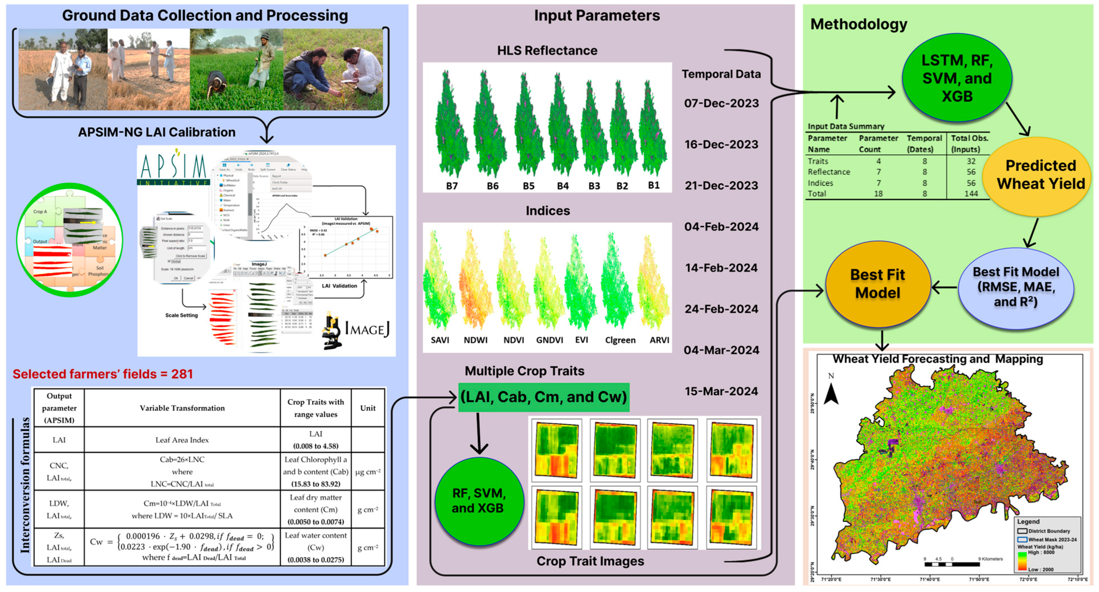
2. Materials and Methods

The methodology for wheat yield prediction comprises four major components: (i) ground data collection and processing, (ii) input parameter preparation, (iii) analysis framework, and (iv) yield forecasting and mapping. The key components of the proposed methodology are shown in Figure 1 and are described below.

2.1. Study Area

The study focused on the Lodhran District, Punjab, Pakistan, a major wheat-producing region contributing approximately 594,700 tons annually from 155,400 hectares, with an average yield of 3827 kg ha⁻¹ [47]. Lodhran was selected due to its standardized administrative reporting hierarchy (district → provincial → national) and accessibility to ground information, high-resolution agricultural records, field boundaries, and agroecological zones, as illustrated in Figure 2.

2.2. Geo-Tagged Ground Data

Geo-referenced farm management data for 281 wheat fields (2023–2024 season) were obtained from the Punjab Agriculture Department, including sowing dates, fertilizer/irrigation schedules, seed sources, plant populations, soil types, and harvest yields [44,48]. Field centroids were converted to 60 × 60 m boundaries (~1 acre) to align with the Harmonized Landsat and Sentinel-2 (HLS) 30 m resolution. Crop traits (LAI, Cab, Cm, and Cw) were simulated using Agriculture Production Systems sIMulator Next Generation (APSIM NG) based on site-specific management inputs [29].

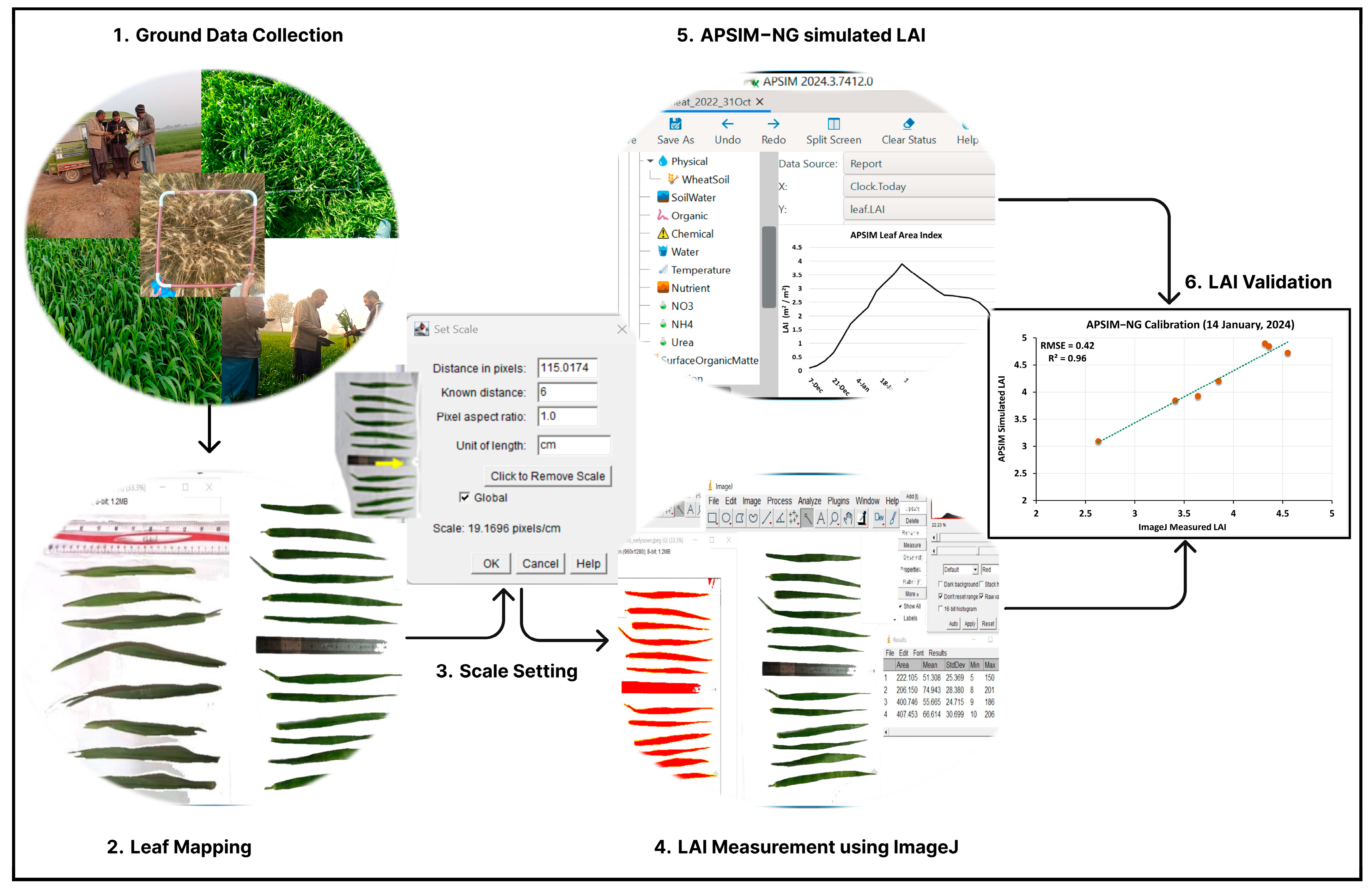
2.3. Calibration of APSIM NG

APSIM NG is an advanced version of APSIM classic 7.10 which simulates crop growth and development through physiologically driven algorithms that integrate daily weather data (minimum/maximum temperature, rainfall, and solar radiation) and crop management inputs [25]. The model has been evaluated and validated globally for wheat, including in Asia and Pakistan [28,49]. The version APSIM NG 2024.3.7412.0 was used to simulate the LAI.

Most crop growth models prioritize the direct simulation of the LAI due to its foundational role in biomass accumulation and light interception [50]. Secondary traits like chlorophyll ab (Cab), leaf dry matter content (Cm), and leaf water content (Cw) were derived using conversion formulas [25]. Consequently, model calibration focused exclusively on optimizing LAI accuracy. The calibration workflow (Figure 3) involved the following steps:

(1)

Parameterization: inputting site-specific management practices (sowing dates and irrigation/fertilizer schedules) and meteorological data;

(2)

Sensitivity analysis: identifying key drivers of LAI variability under local agronomic conditions;

(3)

Validation: comparing simulated LAI against ground-truth measurements to refine physiological coefficients.

This targeted calibration ensured robust LAI estimation, forming the basis for subsequent trait derivations and yield modeling.

2.3.1. Data Collection for LAI

Field campaigns were conducted across seven wheat plots to collect plant density (plants per m²) and leaf area data for LAI calibration. Destructive sampling was performed, and LAI measurements were used to calibrate APSIM NG. Additionally, essential farm management practice data (sowing dates and irrigation/fertilizer schedules) were collected to parameterize LAI simulation in APSIM NG.

2.3.2. Leaf Area Index Measurement

In lieu of specialized equipment (e.g., leaf area meter) unavailability, the leaf area was quantified using ImageJ software (Version 1.54i, Java 1.8 0_345), which proved effective for this purpose [51,52,53]. The plant population was determined by counting the number of plants per m², and three plants were uprooted from each field (destructive sampling) to measure the leaf area. Leaves were detached, spread on white paper with a calibration scale, and photographed. The images were processed in ImageJ, where the scale was used to convert the measurements to pixels per cm. This conversion (pixels/cm) in ImageJ converts the pixel count to real-world units to ensure accurate and consistent leaf area measurements across all images of the study to cater for the variations in magnification or resolution of images during photographing. After conversion to 8-bit and threshold setting, the leaf area is determined by automatically outlining the leaves using the “Wand (tracing) Tool” in ImageJ. The research study also compared the leaf areas measured using the scanner and camera (ImageJ) with a stepwise guide to using ImageJ [53]. The number of plants per m² was multiplied by the average LA of the three plants to obtain the total leaf area and is considered as the LAI due to sampled land area of 1 m².

2.3.3. APSIM NG Simulation and Validation

Prior to initiating simulations in APSIM NG, essential model parameters, particularly those related to soil and wheat varieties, were adjusted in light of the relevant studies conducted in Pakistan [28,29,54,55]. These studies pertained to APSIM wheat constants to sensibly simulate crop growth under high-temperature conditions, specifically for wheat phenology. Key input parameters, including the sowing time, plant population, irrigation, and fertilizer application, were tailored for each farmer to generate the LAI and other relevant parameters on a daily timeframe. The model was validated using accuracy metrics by comparing the LAI measurements from ImageJ with those simulated using APSIM NG on the date of sampling and the field survey.

2.3.4. Derivation of Other Crop Traits

Certain traits, such as the Cab, Cm, and Cw, are difficult to measure in the field, requiring not only destructive sampling but also equipment constraints in addition to being time consuming and labor intensive. To address this, multiple crop trait values within physiologically plausible ranges were derived using a smart solution of variables using transformation formulas (

Table 1. Variable transformation formulas for crop traits.

Output Parameter (APSIM)	Variable Transformation	Crop Traits with Range Values	Unit
LAI	Leaf area index	LAI (0.008 to 4.58)
CNC and LAITotal	Cab = 26 × LNC [56] where LNC = CNC/LAITotal	Leaf chlorophyll a and b content (Cab) (15.83 to 83.92)	µg cm−2
LDW and LAITotal	Cm = 10−4 × LDW/LAITotal where LDW = 10 × LAITotal/SLA [25]	Leaf dry matter content (Cm) (0.0050 to 0.0074)	g cm−2
Zs, LAITotal, and LAIDead	Cw = $=\left\{\begin{array}{c}0.000196·Z_s+0.0298,if{f}_{\mathrm{dead}}=0;\\ 0.0223·\exp \left(-1.90·f_{\mathrm{d}\mathrm{e}\mathrm{a}\mathrm{d}}\right),if{f}_{\mathrm{d}\mathrm{e}\mathrm{a}\mathrm{d}}>0\end{array}\right\}$ where fdead = LAIDead/LAITotal [25]	Leaf water content (Cw) (0.0038 to 0.0275)	g cm−2

). These traits were then utilized for model training and testing to evaluate their performance in crop yield prediction based on the input parameters given in Figure 1, as well as their integration for a holistic understanding of the factors influencing crop yield.

2.4. Reflectance Data

NASA’s Harmonized Landsat and Sentinel-2 (HLS) dataset integrates surface reflectance (SR) data from the Operational Land Imager (OLI) on Landsat 8/9 (L30 product) and the Multi-Spectral Instrument (MSI) on the Sentinel-2 satellite (S30 product) using advanced cross-sensor calibration algorithms [57]. Cloud-free HLS images spanning the wheat growth season (7 December 2023 to 15 March 2024) were processed, although persistent fog during January 2024 precluded usable data from both platforms. The final dataset comprised two L30 images (7 December and 4 March) and six S30 images (16 and 21 December; 4, 14, and 24 February; and 15 March), leveraging harmonized sensor synergy to enhance the temporal resolution beyond individual sensor capabilities.

Reflectance values were averaged within geo-referenced field boundaries (60 m × 60 m) to align with farm-scale management units, mitigating the impact of HLS’s 30 m spatial resolution. Seven common bands, including Aerosol, Blue, Green, Red, Near-Infrared, Shortwave Infrared 1 and 2 of L30 and S30 were retained for consistency across L30 and S30 products. Reflectance data were analyzed both independently and in conjunction with crop traits and indices to evaluate their predictive capacity for wheat yield.

2.5. Vegetation Indices

Vegetation indices (VIs), derived from remote sensing data, are critical tools for monitoring crop characteristics like the LAI, aboveground biomass (AGB), and chlorophyll content, enabling robust yield prediction across heterogeneous landscapes [58,59]. These indices quantify temporal variations in crop vigor and stress, establishing relationships between spectral signatures and productivity [60]. Multi-VI frameworks outperform single-index approaches by capturing complementary physiological signals across growth stages [43,60]. For instance, the EVI correlates with the LAI, resolving saturation issues in dense canopies. Chlorophyll Green (Clgreen) tracks the photosynthetic activity and nitrogen status with the chlorophyll content, and the NDWI assesses canopy moisture dynamics. This diversity in VI metrics is particularly valuable for addressing variabilities across large areas. Leveraging the spectral bands of the HLS dataset, this study employed seven VIs (

Table 2. Vegetation indices with their formulas and impact.

VI Name	Formula	Band Wavelengths (Micrometers)	Impact	Reference
ARVI	(B05 − (2 × B04 − B02))/(B05 + (2 × B04 − B02))	B02 = 0.45–0.51 B04 = 0.64–0.67 B05 = 0.85–0.88	Minimizes effects of atmospheric aerosols	[61]
Clgreen	B05/B03 − 1	B03 = 0.53–0.59 B05 = 0.85–0.88	Sensitive to Cab	[62,63]
EVI	2.5 × (B05 − B04)/ (B05 + 6 × B04 − 7.5 × B02 + 1)	B02 = 0.45–0.51 B04 = 0.64–0.67 B05 = 0.85–0.88	Sensitive to high biomass	[64]
GNDVI	(B05 − B03)/(B05 + B03)	B03 = 0.53–0.59 B05 = 0.85–0.88	Sensitive to LAI	[63,65]
NDVI	(B05 − B04)/(B05 + B04)	B04 = 0.64–0.67 B05 = 0.85–0.88	Density and greenness of vegetation	[66]
NDWI	(B05 − B06)/(B05 + B06)	B05 = 0.85–0.88 B06 = 1.57–1.65	Sensitive to water content	[67]
SAVI	(B05 − B04)/ (B05 + B04 + 0.5) × 1.5	B04 = 0.64–0.67 B05 = 0.85–0.88	Minimizes soil brightness effects	[68]

) to disentangle trait-specific contributions to yield variability while mitigating sensor- and scale-related noise.

2.6. Machine Learning Models

Machine learning enhances crop yield prediction by enabling rapid, data-driven assessments of agricultural supply-demand dynamics, critical for stakeholders’ decision making [69]. Among machine learning algorithms, Random Forest (RF), Support Vector Machine (SVM), Extreme Gradient Boost (XGBoost), and Long Short-Term Memory (LSTM) networks are widely adopted for their ability to resolve nonlinear relationships in heterogeneous agriculture datasets [70]. LSTM, in particular, excels in modeling temporal dependencies with sequential data (e.g., phenological growth states and sensor time series), outperforming traditional models in regional yield estimation [71]. These four algorithms were selected for their complementary strengths in handling spatial, spectral, and temporal yield drivers.

2.6.1. Model Parameters

A total of 18 input parameters consisting of four crop traits (LAI, Cab, Cm, and Cw), seven reflectance bands, and seven indices (Table 2) for eight time steps as per cloud-free HLS data availability were derived for 281 field yield records of geo-tagged farmers provided by the Punjab Agriculture Department. These records were divided into training (80%) and testing (20%) sets to identify the best-fit model for crop yield prediction. The LSTM model leverages time-series information; therefore, a time step links the sequential inputs with the yield output. Accordingly, a matrix format of 8 × 18 (time step × number of input parameters) was used for LSTM, while a 1 × 144 matrix format for each record was applied for the RF, SVM, and XGBoost models.

2.6.2. Model Optimization and Performance Analysis

The LSTM model architecture was experimentally optimized through iterative trials, with the final hyperparameters (e.g., layers, dropout rates, and epochs) detailed in

Table 3. LSTM architecture and configuration.

Layer Index	Layer Type	Units/ Filters	Activation	Input Shape	Output Shape	Additional Configuration
1	LSTM	512	tanh	(8, features)	(8, 512)	-
2	BatchNormalization	N/A	N/A	(8, 512)	(8, 512)	Normalizes outputs of LSTM Layer 1
3	LSTM	256	tanh	(8, 512)	(8, 256)	-
4	BatchNormalization	N/A	N/A	(8, 256)	(8, 256)	Normalizes outputs of LSTM Layer 2
5	LSTM	128	tanh	(8, 256)	(8, 128)	-
6	BatchNormalization	N/A	N/A	(8, 128)	(8, 128)	Normalizes outputs of LSTM Layer 3
7	LSTM	64	tanh	(8, 128)	(64)	Outputs final state only
8	BatchNormalization	N/A	N/A	(64)	(64)	Normalizes outputs of LSTM Layer 4
9	Dropout	N/A	N/A	(64)	(64)	Dropout rate = 0.3
10	Flatten	N/A	N/A	(64)	(64)	Converts output to 1D array
11	Dense (Output)	1	Linear	(64)	(1)	Regression output
Loss Function		MSE (Mean_Squared_Error)
Optimizer		Adam with initial learning rate = 0.001
Training Configuration		Batch Size: 32 Epochs: 500 Early Stopping with Patience = 100 and Restore Best Weights: True Shuffle: True

. Input data were pre-processed via min–max normalization to ensure scale invariance.

However other models were optimized using a grid search combined with cross-validation. For the RF and XGBoost models, 5-fold cross-validation was used to optimize the tuning parameters, while the SVM model was optimized via 10-fold cross-validation to refine the kernel coefficients and penalty terms. The hypermeter tuning of each model against the input parameter is given in

Table 4. Hyperparameters for the RF, SVM, and XGBoost models against the parameters.

Hyperparameters	Integrated	Crop Traits	Reflectance	Indices
Random Forest
Min Sample Leaf	3	3	4	2
Min Sample Split	10	10	10	10
n-estimator	250	100	250	200
OOB Error	96,739	94,658.2	276,245.1	277,724.5
Support Vector Machine
C	1	1	1	1
Gamma	0.0069	0.0312	0.0179	0.0179
Kernel	radial	radial	radial	radial
Epsilon	0.1	0.1	0.1	0.1
Extreme Gradient Boost
Learning Rate	0.001	0.01	0.01	0.2
Max Depth	3	3	3	3
Regular Lambda	1	0.1	1	0
n-estimator	300	300	200	200

. This approach contributed to the models’ robustness and reliability, improving predictive accuracy and generalization ability. The models’ performances were evaluated using the Root Mean Squared Error (RMSE), Mean Absolute Error (MAE), and coefficient of determination R² metrics.

2.7. Wheat Yield Forecasting and Mapping

For the best fit based on evaluation criteria, a trained model was used to forecast the wheat yield across the study area. To map crop traits across the study area, trained models of a SVM, XGBoost, and RF of the study [52] were implemented on HLS reflectance for the prediction of crop traits to obtain a wheat yield mapping framework, as given in Figure 1. This approach aligns with advancements in geospatial crop mapping that integrate heterogeneous datasets (e.g., satellite imagery and trait proxies) to resolve agroecological heterogeneity [63,72,73].

3. Results

3.1. Model Accuracy Assessment

The ability of crop traits, reflectance, and vegetation indices and their integration to predict wheat yield using machine learning models was evaluated.

Table 5. Model performance comparison.

Model	Evaluation Criteria
	RMSE (kg/ha)	MAE (kg/ha)	R2
Integrated (crop traits + reflectance + indices)
LSTM	250.68	193.76	0.84
RF	293.56	230.68	0.78
SVM	309.8	231.45	0.75
XGB	303.25	239.64	0.76
Crop traits
LSTM	278.11	214.65	0.80
RF	291.73	223.17	0.78
SVM	317.37	236.10	0.74
XGB	326.04	251.29	0.72
Reflectance
LSTM	462.80	349.07	0.44
RF	501.68	396.44	0.34
SVM	522.39	383.25	0.29
XGB	488.87	398.15	0.38
Indices
LSTM	470.04	366.72	0.42
RF	513.52	406.00	0.31
SVM	525.35	383.05	0.28
XGB	502.59	398.65	0.34

summarizes the performance comparison among the machine learning models for crop traits, reflectance, indices, and their integration to predict wheat crop yield. Model predictions against test data for different input parameters are visualized in Figure 4. Among the models, LSTM demonstrated the best-fit prediction across all input parameters (Table 5), followed by the RF model. All models (LSTM, RF, XGBoost, and SVM) performed within the prediction ranges reported in the literature, confirming their suitability for wheat yield prediction [74,75]. The evaluation metrics (RMSE, MAE, and R²) revealed that LSTM achieved superior accuracy for the integrated parameters primarily due to its advantage in handling long-term dependencies and temporal dynamics critical for capturing crop variability [71].

Consistent with the methodological framework, integrating parameters and crop traits yielded the best performance, demonstrating the advantage of parameter integration in capturing intra-and inter-field yield variation information. LSTM performed best with the integrated input parameters, followed by the RF model. XGBoost outperformed the SVM but lagged behind LSTM and the RF, as detailed in Table 5. LSTM exhibited more precise predictions across yield ranges, particularly for lower values, where other models performed less accurately (Figure 4). Parameter integration improved the RMSE by 9% compared to crop traits alone and by 45% over the reflectance and indices, while the R² increased by 5% over the crop traits and nearly doubled compared to the reflectance and indices alone.

Crop trait-based wheat yield predictions exhibited performances comparable to the integrated parameters, with minor differences demonstrating dominance over other input types. LSTM performed best for wheat yield prediction based on crop traits, followed by the RF model. Notably, the RF model showed marginally better performance with crop traits than integrated parameters. However, the LSTM model demonstrated superior precision for lower yield values when using integrated parameters. The SVM and XGBoost exhibited similar performances, with slight variations in the evaluation criteria (Table 5).

Reflectance and index-based yield predictions underperformed relative to the integrated and trait-based approaches, although limited studies have documented accuracy within this range [74,75]. This low accuracy may be due to satellite data quality issues, including spectral saturation in dense canopies and atmospheric noise. Reflectance-based crop yield predictions had RMSEs ranging from 462.80 to 522.39 kg/ha, MAEs from 349.07 to 398.15 kg/ha, and R²s from 0.29 to 0.44. Despite these challenges, LSTM remained the top performer for reflectance-based yield prediction, followed by XGBoost, as shown in Table 5. Indices, being the derived product of satellite reflectance, exhibited similar performance. Index-based yield prediction had RMSEs ranging from 470.04 to 525.35 kg/ha, MAEs from 366.72 to 398.65 kg/ha, and R²s from0.28 to 0.42. LSTM again showed the best performance for index-based yield prediction. Index-based yield prediction showed the lowest performance. Among the models, XGBoost showed better prediction accuracy as compared to the RF and SVM models for both reflectance and index-based prediction. This advantage of XGBoost can be attributed to its ability to handle sparse and noisy data more effectively.

3.2. Wheat Yield Forecasting and Mapping

Crop traits (LAI, Cab, Cm, and Cw) were predicted following the methodology outlined in Figure 1. Based on trained models previously developed [52], crop trait maps were produced for all requisite dates to generate input parameters for the entire study area. Given its superior performance as per the evaluation criteria for integrated input parameters (crop traits, reflectance, and indices), the LSTM model was employed to forecast and map the yield across the district Lodhran. Figure 5 shows the 2023–2024 wheat yield map for Lodhran, identifying site-specific variations not only for low- and high-yield areas but also within-field yield variations. This map provides actionable insights for improving the yield through targeted management practices in low-productivity intra- and inter-field areas.

The district-level average yield, derived from pixel-wise analysis, was estimated at 3746.36 kg/ha against the preliminary reported yield of 3961 kg/ha for 2023–2024 by the Punjab Agriculture Department (validation of the final official estimate remains pending). The results demonstrated the model’s robustness, with a 5.4% deviation from preliminary statistics, while highlighting the advantages of resource efficiency and geospatial pixel-based yield information based on multi-trait integration. Although the methodology from the Punjab Agriculture Department is a reliable benchmark, its reliance on small-plot sampling (6 × 8 ft) introduces limitations in a heterogeneous field [44]. For example, pixel-wise field yield prediction (Figure 6) reveals that the selected sampling area may vary for the yield across fields. Fields 2, 195, 116, and 114 display uniform yields across pixels, making a single sampling point representative of the whole field. Conversely, Fields 66, 198, 120, and 208 exhibit significant intra-field yield variation, where isolated sampling could misrepresent the field’s overall productivity. Field 120, in particular, showed yield variation across all pixels, indicating that single-point sampling is inadequate to represent the average yield or generalize across larger areas. Thus, a large sample size instead of a small (6 × 8 ft) one can mitigate biases inherent in the current methodology. Furthermore, the regions demarcated in Figure 5 (Boxes 1, 2, and 3) delineate high-, average-, and low-yield zones, respectively, offering spatially explicit guidance for precision agriculture interventions.

4. Discussion

4.1. Machine Learning Model Performance Comparison

The performance differences across models and data types highlight the strengths and limitations of each approach. Among the machine learning models, LSTM consistently outperformed others, especially in integrating multi-source data. This superiority likely stems from LSTM’s capacity to capture sequential dependencies and temporal patterns inherent in crop traits and yield data, which are intrinsically linked to phenological growth stages [76]. The advantage of LSTM for index- and reflectance-based wheat yield prediction lies in its ability to incorporate temporal fluctuations in crop health and growth stage changes during the growing season. LSTM’s optimal performance can be attributed to its network architecture with the configuration given in Table 3, specifically designed for model temporal dependencies, which is a crucial factor in yield prediction, as yield-influential variables exhibit a time-sensitive impact on crop development [76]. The yield development trajectory depends on its growth, particularly at critical phenological stages. Any growth variation during the season is reflected in the crop yield, making LSTM ideally suited for analyzing sequential changes. Moreover, LSTM also effectively handles the complexity of input parameter integration due to its ability to model long-term dependencies [76].

Conversely, other models like the RF, SVM, and XGB, although capable of handling high-dimensional, complex data, lack inherent mechanisms to interpret time-dependent relationships between inputs and yield [76]. These findings align with prior studies, where LSTM surpassed the RF, GBDT, and SVR models in wheat yield estimation [71]. However, earlier work focused on high-resolution (5 m × 5 m) gridded yield data from 15,709 observations from a small area with similar management practices. In contrast, this study spans a broader and more diverse field area, encompassing multiple wheat fields with diverse management resources and practices. This approach provides a more comprehensive representative of actual field conditions, supporting actionable decision making and policy formulation for yield optimization.

The RF also demonstrated strong performance, although it was slightly less effective than LSTM in capturing complex patterns, particularly when integrating multiple data types. Its higher performance in crop trait-based yield prediction can be attributed to its ensemble approach, which resolves nonlinear and intricate relationships between traits and yield through aggregated decision trees [77]. XGBoost demonstrated competitive performance, particularly for reflectance and index data, likely owing to its robustness against noisy and sparsity, which are common challenges in satellite-derived datasets affected by factors like cloud cover, sunlight variability, and atmospheric conditions [78]. Consequently, for reflectance and index-based wheat yield prediction, XGBoost performed better than the RF and SVM.

Among the input parameters, multiple crop traits demonstrate strong potential for efficient crop yield. These traits capture phenotypic and physiological features because of their functional relationship with crop growth and development that directly affect crop yields. The LAI and Cab’s role in capturing radiation assisted by Cm for radiation conversion to biomass and Cw support for stress during the season highlight their role as the most informative predictors for yield prediction. Additionally, being multiple traits, they cumulatively exhibit a precise direct connection with photosynthesis [79], climatic conditions [12], and crop management practices [13], which collectively govern yield potential. Even in crop breeding programs, crop traits or their combinations determine yield potential assessment through crop growth models informed by field experimentation and crop physiology [80], underscoring their predictive value. However, efficient and scalable methods for multi-trait estimation remain critical, as demonstrated by the integrative approach used in this study.

In contrast, reflectance and vegetation indices performed less effectively as standalone predictors, particularly for SVM and RF models. This limitation arises because their correlation with yield depends on farm management practices, environmental conditions, and crop growth stage in addition to atmospheric conditions and spectral saturation at high canopy crop cover [59]. Despite the relatively weaker performance of reflectance and indices as standalone inputs, their integration with crop traits showed a slight improvement in model performance (ΔRMSE = 27.43 kg/ha; ΔR² = 0.04). This suggests that reflectance and indices provide valuable complementary information when used in conjunction with crop traits in addition to the spatial coverage [81]. For example, reflectance data could capture environmental stresses or canopy structure variations that crop traits alone might miss, enabling model generalizability across diverse conditions [82]. This synergy, combined with the spatial coverage of remote sensing, strengthens the framework’s applicability for precision agriculture.

4.2. Wheat Yield Variability Factor

Wheat yield mapping revealed distinct intra-and inter-yield variability across the Lodhran district, with pronounced disparities between high- and low-yield zones. As shown in the boxes in Figure 5, Box 1 represents a high-yield area, Box 3 represents a low-yield area, and Box 2 is a transitional area with mixed productivity. The presence of low-wheat-yield areas in Box 1 and Box 2 potentially indicates suboptimal management practices. Utilizing this map enables targeted, site-specific crop management interventions to minimize intra- and inter-yield variations, thus enhancing wheat crop productivity across the district. Thus, it is an effective input to support precision agriculture implementation.

Moreover, a distinct low yield in the lower right section, including Box 3, indicates systemic constraints affecting large-scale productivity. The limiting factor was identified to support and validate the findings of the study. The limiting factor observed was the brackish groundwater with less than the required canal water supply during the rabi season of 2023–2024. According to the Soil Fertility Research Institute (SFRI) Punjab, Lahore, electrical conductivity (EC) levels exceed 1250 µS/cm across most of the district, rendering the groundwater unsuitable for irrigation (Figure 7). Only a narrow zone along the Sutlej riverine exhibited marginally acceptable EC levels (1001–1250 µS/cm). Groundwater with EC levels suitable for irrigation (<1001 µS/cm) is confined to terraces near the Sutlej. Consequently, the crop productivity of the district relies heavily on the availability of canal water supply. The district is irrigated by two main canals, namely the Lower Pakpattan Canal (LPC) and Lower Mailsi Canal (LMC) [83]. The LPC irrigates the upper left part (high wheat yield area) and has more than 60% of the area under the perennial command area, whereas the LMC irrigates the lower right part (low wheat yield area) and has only 32% of the area under perennial and the majority under non-perennial command area. Limited canal water allocation to the LMC during the 2023–2024 rabi season exacerbated water scarcity in this region, compounding challenges posed by brackish groundwater [83]. This dual constraint, poor water quality and inadequate canal supply, explain the stark productivity gradient observed in Figure 5.

For the rabi season 2023–2024, the proposed water shares, entitlements, and deliveries are detailed in

Table 6. Canal water supply situation rabi 2023–2024.

Canal Name	Canal-Wise Irrigation Water Supplies (MAF) Rabi 2023–2024
	Proposed	Entitled	Delivered	% Over-Proposed	% Over-Entitled
Lower Pakpattan Canal (LPC)	0.347	0.211	0.376	7.7	43.9
Lower Mailsi Canal (LMC)	0.349	0.238	0.288	−21.2	17.4

[84]. As per the Punjab Irrigation Department records, the LPC received 7.7% above the proposed allocations and 43.9% above the entitlement shares. In contrast, the LMC received 21.2% below the proposed allocations and 17.4% above the entitlement shares during the same period. This disparity in water distribution, coupled with the LPC’s predominance of non-perennial irrigation zones, explains the pronounced wheat yield deficit in the district’s lower right sector [83,84]. This irrigation shortage directly impacted crop growth, manifesting as reduced leaf water content (Cw), a key trait linked to drought and salinity stress resilience. To mitigate yield losses, stakeholders must prioritize interventions such as infrastructure upgrades to improve canal water equity and reliability, the promotion of salt-tolerant wheat cultivars adapted to brackish groundwater conditions, and the adoption of water-efficient practices (e.g., drip irrigation and soil moisture sensors) to optimize resource use. Such measures would enhance the net margins for farmers in water-stressed regions while addressing systemic productivity constraints.

4.3. Limitations

Crop harvest sampling aligned with pixel dimension and geolocation or standardized one-hectare sampling units (the base unit for yield measurement) could enhance model robustness and efficiency. This is because yield specific to pixel reflectance establishes a precise and comprehensive relation between reflectance and yield. Similarly, using a one-hectare base area representation helps minimize the impact of intra-field variations caused by inputs within the base area. Additionally, reflectance data and indices are often subject to atmospheric interference and noise, potentially affecting the precision and generalizability of crop yield prediction in different regions. Another limitation stems from the potential misclassification in the wheat mask, where some areas might include other crops, particularly fodder crops. This misclassification could slightly skew high- or low-yield mapping, as different crops can introduce variability in the reflectance and indices.

5. Conclusions

This study presents an optimized approach for wheat yield prediction by integrating multi-traits physiological data (LAI, Cab, Cm, and Cw), satellite reflectance, vegetation indices, and machine learning models (LSTM, RF, XGBoost, and SVM). The model achieved a 5.4% variation from the reported yield at the district level, demonstrating that multi-trait integration comprehensively accounted for growth-stage variations across large spatial scales. The results underscore crop traits as pivotal drivers of model performance, underscoring a valuable research avenue to develop precise yield models centered around diverse crop traits. While multi-trait approaches remain underexplored, often due to data scarcity or estimation complexity, advancements in crop growth models or transformation formulas could unlock their full predictive power.

Despite reflectance and indices underperforming as standalone predictors, their integration with crop traits contributed to robustness and accuracy improvement, with LSTM emerging as the most effective model for resolving temporal dependencies. The integration provides a more holistic view of the complex factors influencing crop yield, enhancing the model’s accuracy and generalization in addition to the potential for improvement in resilience to variability in environmental conditions. Moreover, the implementation of scalable yield estimation and mapping in relevant agriculture statistics forums, particularly in Pakistan, will provide reliable and precise spatial estimation. Additionally, it will support effective decision making to support relevant stakeholders for site-specific measures as per intra-and inter-field variations in crop yield and production. The incorporation of more temporal, diverse datasets particularly relevant to crop growth behavior and integration techniques can further improve the performance and generalizability of crop yield models from within the field to the regional level in the future.

References

1. Pantazi, X.E.; Moshou, D.; Alexandridis, T.; Whetton, R.L.; Mouazen, A.M. Wheat Yield Prediction Using Machine Learning and Advanced Sensing Techniques. Comput. Electron. Agric. 2016, 121, 57–65. [Google Scholar] [CrossRef]
2. Holzman, M.E.; Carmona, F.; Rivas, R.; Niclòs, R. Early Assessment of Crop Yield from Remotely Sensed Water Stress and Solar Radiation Data. ISPRS J. Photogramm. Remote Sens. 2018, 145, 297–308. [Google Scholar] [CrossRef]
3. Whetton, R.; Zhao, Y.; Shaddad, S.; Mouazen, A.M. Nonlinear Parametric Modelling to Study How Soil Properties Affect Crop Yields and NDVI. Comput. Electron. Agric. 2017, 138, 127–136. [Google Scholar] [CrossRef]
4. Dash, Y.; Mishra, S.K.; Panigrahi, B.K. Rainfall Prediction for the Kerala State of India Using Artificial Intelligence Approaches. Comput. Electr. Eng. 2018, 70, 66–73. [Google Scholar] [CrossRef]
5. Lek, S.; Delacoste, M.; Baran, P.; Dimopoulos, I.; Lauga, J.; Aulagnier, S. Application of Neural Networks to Modelling Nonlinear Relationships in Ecology. Ecol. Modell. 1996, 90, 39–52. [Google Scholar] [CrossRef]
6. Neetu, R.; Bamel, K.; Abhinav, S.; Singh, N. Analysis of Five Mathematical Models for Crop Yield Prediction. South Asian J. Exp. Biol. 2022, 12, 46–54. [Google Scholar] [CrossRef]
7. Bandaru, V.; Yaramasu, R.; Jones, C.; César Izaurralde, R.; Reddy, A.; Sedano, F.; Daughtry, C.S.T.; Becker-Reshef, I.; Justice, C. Geo-CropSim: A Geo-Spatial Crop Simulation Modeling Framework for Regional Scale Crop Yield and Water Use Assessment. ISPRS J. Photogramm. Remote Sens. 2022, 183, 34–53. [Google Scholar] [CrossRef]
8. Wang, L.; Chen, S.; Peng, Z.; Huang, J.; Wang, C.; Jiang, H.; Zheng, Q.; Li, D. Phenology Effects on Physically Based Estimation of Paddy Rice Canopy Traits from UAV Hyperspectral Imagery. Remote Sens. 2021, 13, 1792. [Google Scholar] [CrossRef]
9. Arakeri, M.P.; Vijaya Kumar, B.P.; Barsaiya, S.; Sairam, H.V. Computer Vision Based Robotic Weed Control System for Precision Agriculture. In Proceedings of the 2017 International Conference on Advances in Computing, Communications and Informatics (ICACCI), Udupi, India, 13–16 September 2017; IEEE: New York, NY, USA; pp. 1201–1205. [Google Scholar]
10. Phuoc, L.H.; Suliansyah, I.; Arlius, F.; Chaniago, I.; Xuan, N.T.T.; Quang, P. Van Literature Review Crop Modeling and Introduction a Simple Crop Model. J. Appl. Agric. Sci. Technol. 2023, 7, 197–216. [Google Scholar] [CrossRef]
11. Chang, Y.; Latham, J.; Licht, M.; Wang, L. A Data-Driven Crop Model for Maize Yield Prediction. Commun. Biol. 2023, 6, 439. [Google Scholar] [CrossRef]
12. Harbinson, J.; Yin, X. Modelling the Impact of Improved Photosynthetic Properties on Crop Performance in Europe. Food Energy Secur. 2023, 12, e402. [Google Scholar] [CrossRef]
13. Gorooei, A.; Gaiser, T.; Aynehband, A.; Rahnama, A.; Kamali, B. The Effect of Farming Management and Crop Rotation Systems on Chlorophyll Content, Dry Matter Translocation, and Grain Quantity and Quality of Wheat (Triticum aestivum L.) Grown in a Semi-Arid Region of Iran. Agronomy 2023, 13, 1007. [Google Scholar] [CrossRef]
14. Xie, Y.; Wang, P.; Bai, X.; Khan, J.; Zhang, S.; Li, L.; Wang, L. Assimilation of the Leaf Area Index and Vegetation Temperature Condition Index for Winter Wheat Yield Estimation Using Landsat Imagery and the CERES-Wheat Model. Agric. For. Meteorol. 2017, 246, 194–206. [Google Scholar] [CrossRef]
15. Lambert, M.-J.; Traoré, P.C.S.; Blaes, X.; Baret, P.; Defourny, P. Estimating Smallholder Crops Production at Village Level from Sentinel-2 Time Series in Mali’s Cotton Belt. Remote Sens. Environ. 2018, 216, 647–657. [Google Scholar] [CrossRef]
16. Singh, R.; Krishnan, P.; Singh, V.K.; Sah, S.; Das, B. Combining Biophysical Parameters with Thermal and RGB Indices Using Machine Learning Models for Predicting Yield in Yellow Rust Affected Wheat Crop. Sci. Rep. 2023, 13, 18814. [Google Scholar] [CrossRef]
17. Choudhary, K.; Shi, W.-Z.J.; Kupriyanov, A.; Boori, M.S. A Brief Overview of Satellite Imagery for Yield Estimation in Agroecosystem. In Proceedings of the 2022 VIII International Conference on Information Technology and Nanotechnology (ITNT), Samara, Russian, 23–27 May 2022; IEEE: New York, NY, USA; pp. 1–6. [Google Scholar]
18. Pignatti, S.; Casa, R.; Laneve, G.; Li, Z.; Liu, L.; Marzialetti, P.; Mzid, N.; Pascucci, S.; Silvestro, P.C.; Tolomio, M.; et al. Sino–EU Earth Observation Data to Support the Monitoring and Management of Agricultural Resources. Remote Sens. 2021, 13, 2889. [Google Scholar] [CrossRef]
19. Apolo-Apolo, O.E.; Pérez-Ruiz, M.; Martínez-Guanter, J.; Egea, G. A Mixed Data-Based Deep Neural Network to Estimate Leaf Area Index in Wheat Breeding Trials. Agronomy 2020, 10, 175. [Google Scholar] [CrossRef]
20. Kanning, M.; Kühling, I.; Trautz, D.; Jarmer, T. High-Resolution UAV-Based Hyperspectral Imagery for LAI and Chlorophyll Estimations from Wheat for Yield Prediction. Remote Sens. 2018, 10, 2000. [Google Scholar] [CrossRef]
21. Wang, Y.; Yin, Y. Agriculture in Silico: Perspectives on Radiative Transfer Optimization Using Vegetation Modeling. Crop Environ. 2023, 2, 175–183. [Google Scholar] [CrossRef]
22. Szabó, É. Relationship between the Physiological Properties and Yield of Winter Wheat Varieties on Chernozem Soil. Acta Agron. Hungarica 2013, 61, 279–292. [Google Scholar] [CrossRef]
23. Poorter, H.; Niinemets, Ü.; Poorter, L.; Wright, I.J.; Villar, R. Causes and Consequences of Variation in Leaf Mass per Area (LMA): A Meta-analysis. New Phytol. 2009, 182, 565–588. [Google Scholar] [CrossRef] [PubMed]
24. Sieling, K.; Böttcher, U.; Kage, H. Dry Matter Partitioning and Canopy Traits in Wheat and Barley under Varying N Supply. Eur. J. Agron. 2016, 74, 1–8. [Google Scholar] [CrossRef]
25. Chen, Q.; Zheng, B.; Chen, T.; Chapman, S.C. Integrating a Crop Growth Model and Radiative Transfer Model to Improve Estimation of Crop Traits Based on Deep Learning. J. Exp. Bot. 2022, 73, 6558–6574. [Google Scholar] [CrossRef]
26. Li, L.; Guo, N.; Feng, Y.; Duan, M.; Li, C. Effect of Piriformospora indica-Induced Systemic Resistance and Basal Immunity Against Rhizoctonia cerealis and Fusarium graminearum in Wheat. Front. Plant Sci. 2022, 13, 836940. [Google Scholar] [CrossRef]
27. Song, Y.; Rui, F.; Ji, R.; Wu, J.; Yu, W.; Wang, J.; Wang, Y. Impact Analysis of LAI Parameters on Yield Evaluation of RS-P-YEC Model. In Proceedings of the Second International Conference on Geographic Information and Remote Sensing Technology (GIRST 2023), Qingdao, China, 21–23 July 2023; Bilal, M., Tosti, F., Eds.; SPIE: Bellingham, WA, USA; p. 84. [Google Scholar]
28. Shahid, M.R.; Wakeel, A.; Ullah, M.S.; Gaydon, D.S. Identifying Changes to Key APSIM-Wheat Constants to Sensibly Simulate High Temperature Crop Response in Pakistan. Field Crop. Res. 2024, 307, 109265. [Google Scholar] [CrossRef]
29. Wajid, A.; Hussain, K.; Ilyas, A.; Habib-Ur-rahman, M.; Shakil, Q.; Hoogenboom, G. Crop Models: Important Tools in Decision Support System to Manage Wheat Production under Vulnerable Environments. Agriculture 2021, 11, 1166. [Google Scholar] [CrossRef]
30. Thakkar, M.; Vanzara, R. Enhancing Crop Yield Estimation from Remote Sensing Data: A Comparative Study of the Quartile Clean Image Method and Vision Transformer. Discov. Appl. Sci. 2024, 6, 610. [Google Scholar] [CrossRef]
31. Joshi, A.; Pradhan, B.; Gite, S.; Chakraborty, S. Remote-Sensing Data and Deep-Learning Techniques in Crop Mapping and Yield Prediction: A Systematic Review. Remote Sens. 2023, 15, 2014. [Google Scholar] [CrossRef]
32. Du, X.; Zhu, J.; Xu, J.; Li, Q.; Tao, Z.; Zhang, Y.; Wang, H.; Hu, H. Remote Sensing-Based Winter Wheat Yield Estimation Integrating Machine Learning and Crop Growth Multi-Scenario Simulations. Int. J. Digit. Earth 2025, 18, 2443470. [Google Scholar] [CrossRef]
33. Zhang, G.; Roslan, S.N.A.B.; Shafri, H.Z.M.; Zhao, Y.; Wang, C.; Quan, L. Predicting Wheat Yield from 2001 to 2020 in Hebei Province at County and Pixel Levels Based on Synthesized Time Series Images of Landsat and MODIS. Sci. Rep. 2024, 14, 16212. [Google Scholar] [CrossRef]
34. Yang, X.; Zhang, J.H.; Yang, S.S.; Wang, J.W.; Bai, Y.; Zhang, S. Modelling the Crop Yield Gap with a Remote Sensing-Based Process Model: A Case Study of Winter Wheat in the North China Plain. J. Integr. Agric. 2023, 22, 2993–3005. [Google Scholar] [CrossRef]
35. Kartal, S.; Iban, M.C.; Sekertekin, A. Next-Level Vegetation Health Index Forecasting: A ConvLSTM Study Using MODIS Time Series. Environ. Sci. Pollut. Res. 2024, 31, 18932–18948. [Google Scholar] [CrossRef]
36. Roznik, M.; Boyd, M.; Porth, L. Improving Crop Yield Estimation by Applying Higher Resolution Satellite NDVI Imagery and High-Resolution Cropland Masks. Remote Sens. Appl. Soc. Environ. 2022, 25, 100693. [Google Scholar] [CrossRef]
37. Han, X.; Wei, Z.; Chen, H.; Zhang, B.; Li, Y.; Du, T. Inversion of Winter Wheat Growth Parameters and Yield Under Different Water Treatments Based on UAV Multispectral Remote Sensing. Front. Plant Sci. 2021, 12, 609876. [Google Scholar] [CrossRef]
38. Jin, X.B.; Yang, N.X.; Wang, X.Y.; Bai, Y.T.; Su, T.L.; Kong, J.L. Hybrid Deep Learning Predictor for Smart Agriculture Sensing Based on Empirical Mode Decomposition and Gated Recurrent Unit Group Model. Sensors 2020, 20, 1334. [Google Scholar] [CrossRef]
39. van Klompenburg, T.; Kassahun, A.; Catal, C. Crop Yield Prediction Using Machine Learning: A Systematic Literature Review. Comput. Electron. Agric. 2020, 177, 105709. [Google Scholar] [CrossRef]
40. Kulyal, M.; Saxena, P. Machine Learning Approaches for Crop Yield Prediction: A Review. In Proceedings of the 2022 7th International Conference on Computing, Communication and Security (ICCCS), Seoul, Republic of Korea, 3–5 November 2022. [Google Scholar] [CrossRef]
41. Sadenova, M.; Beisekenov, N.; Varbanov, P.S.; Pan, T. Application of Machine Learning and Neural Networks to Predict the Yield of Cereals, Legumes, Oilseeds and Forage Crops in Kazakhstan. Agriculture 2023, 13, 1195. [Google Scholar] [CrossRef]
42. Newlands, N.K.; Zamar, D.S.; Kouadio, L.A.; Zhang, Y.; Chipanshi, A.; Potgieter, A.; Toure, S.; Hill, H.S.J. An Integrated, Probabilistic Model for Improved Seasonal Forecasting of Agricultural Crop Yield under Environmental Uncertainty. Front. Environ. Sci. 2014, 2, 17. [Google Scholar] [CrossRef]
43. Kouadio, L.; Newlands, N.; Davidson, A.; Zhang, Y.; Chipanshi, A. Assessing the Performance of MODIS NDVI and EVI for Seasonal Crop Yield Forecasting at the Ecodistrict Scale. Remote Sens. 2014, 6, 10193–10214. [Google Scholar] [CrossRef]
44. Qayyum, A. Model Based Wheat Yield; GC University Lahore: Lahore, Pakistan, 2011. [Google Scholar]
45. Chlingaryan, A.; Sukkarieh, S.; Whelan, B. Machine Learning Approaches for Crop Yield Prediction and Nitrogen Status Estimation in Precision Agriculture: A Review. Comput. Electron. Agric. 2018, 151, 61–69. [Google Scholar] [CrossRef]
46. Gutman, G.; Skakun, S.; Gitelson, A. Revisiting the Use of Red and Near-Infrared Reflectances in Vegetation Studies and Numerical Climate Models. Sci. Remote Sens. 2021, 4, 100025. [Google Scholar] [CrossRef]
47. Ministry of National Food Security and Research (Economic Wing). Government of Pakistan Crops Area & Production (District Wise) 2022–2023; Ministry of National Food Security and Research (Economic Wing): Islamabad, Pakistan, 2024.
48. Qayyum, A.; Jamil Shera, H.M.M. Method of Area Frame Sampling Using Probability Proportional to Size Sampling Technique for Crops’ Surveys: A Case Study in Pakistan. J. Exp. Agric. Int. 2019, 41, 1–10. [Google Scholar] [CrossRef]
49. Gaydon, D.S.; Balwinder-Singh; Wang, E.; Poulton, P.L.; Ahmad, B.; Ahmed, F.; Akhter, S.; Ali, I.; Amarasingha, R.; Chaki, A.K.; et al. Evaluation of the APSIM Model in Cropping Systems of Asia. Field Crops Res. 2017, 204, 52–75. [Google Scholar] [CrossRef]
50. Ishaq, R.A.F.; Zhou, G.; Tian, C.; Tan, Y.; Jing, G.; Jiang, H.; Obaid-ur-Rehman. A Systematic Review of Radiative Transfer Models for Crop Yield Prediction and Crop Traits Retrieval. Remote Sens. 2024, 16, 121. [Google Scholar] [CrossRef]
51. Martin, T.N.; Fipke, G.M.; Winck, J.E.M.; Marchese, J.A. ImageJ Software as an Alternative Method for Estimating Leaf Area in Oats. Acta Agron. 2020, 69, 162–169. [Google Scholar] [CrossRef]
52. Ahmad, R.; Ishaq, F.; Zhou, G.; Ali, A.; Roshaan, S.; Shah, A.; Jiang, C.; Ma, Z.; Sun, K.; Jiang, H. A Synergistic Framework for Coupling Crop Growth, Radiative Transfer, and Machine Learning to Estimate Wheat Crop Traits in Pakistan. Remote Sens. 2024, 16, 4386. [Google Scholar] [CrossRef]
53. Koyama, K. Leaf Area Estimation by Photographing Leaves Sandwiched between Transparent Clear File Folder Sheets. Horticulturae 2023, 9, 709. [Google Scholar] [CrossRef]
54. Azmat, M.; Ilyas, F.; Sarwar, A.; Huggel, C.; Vaghefi, S.A.; Hui, T.; Qamar, M.U.; Bilal, M.; Ahmed, Z. Impacts of Climate Change on Wheat Phenology and Yield in Indus Basin, Pakistan. Sci. Total Environ. 2021, 790, 148221. [Google Scholar] [CrossRef]
55. Hussain, J.; Khaliq, T.; Ahmad, A.; Akhtar, J. Performance of Four Crop Model for Simulations of Wheat Phenology, Leaf Growth, Biomass and Yield across Planting Dates. PLoS ONE 2018, 13, e0197546. [Google Scholar] [CrossRef]
56. Yang, G.; Zhao, C.; Pu, R.; Feng, H.; Li, Z.; Li, H.; Sun, C. Leaf Nitrogen Spectral Reflectance Model of Winter Wheat (Triticum aestivum) Based on PROSPECT: Simulation and Inversion. J. Appl. Remote Sens. 2015, 9, 095976. [Google Scholar] [CrossRef]
57. Claverie, M.; Ju, J.; Masek, J.G.; Dungan, J.L.; Vermote, E.F.; Roger, J.C.; Skakun, S.V.; Justice, C. The Harmonized Landsat and Sentinel-2 Surface Reflectance Data Set. Remote Sens. Environ. 2018, 219, 145–161. [Google Scholar] [CrossRef]
58. Jamali, M.; Soufizadeh, S.; Yeganeh, B.; Emam, Y. Wheat Leaf Traits Monitoring Based on Machine Learning Algorithms and High-Resolution Satellite Imagery. Ecol. Inform. 2023, 74, 101967. [Google Scholar] [CrossRef]
59. Tiruneh, G.A.; Meshesha, D.T.; Adgo, E.; Tsunekawa, A.; Haregeweyn, N.; Fenta, A.A.; Reichert, J.M. A Leaf Reflectance-Based Crop Yield Modeling in Northwest Ethiopia. PLoS ONE 2022, 17, e0269791. [Google Scholar] [CrossRef]
60. Vidican, R.; Mălinaș, A.; Ranta, O.; Moldovan, C.; Marian, O.; Ghețe, A.; Ghișe, C.R.; Popovici, F.; Cătunescu, G.M. Using Remote Sensing Vegetation Indices for the Discrimination and Monitoring of Agricultural Crops: A Critical Review. Agronomy 2023, 13, 3040. [Google Scholar] [CrossRef]
61. Kaufman, Y.J.; Tanre, D. Atmospherically Resistant Vegetation Index (ARVI) for EOS-MODIS. IEEE Trans. Geosci. Remote Sens. 1992, 30, 261–270. [Google Scholar] [CrossRef]
62. Gitelson, A.A.; Keydan, G.P.; Merzlyak, M.N. Three-band Model for Noninvasive Estimation of Chlorophyll, Carotenoids, and Anthocyanin Contents in Higher Plant Leaves. Geophys. Res. Lett. 2006, 33. [Google Scholar] [CrossRef]
63. Ji, J.; Wang, X.; Ma, H.; Zheng, F.; Shi, Y.; Cui, H.; Zhao, S. Synchronous Retrieval of Wheat Cab and LAI from UAV Remote Sensing: Application of the Optimized Estimation Inversion Framework. Agronomy 2024, 14, 359. [Google Scholar] [CrossRef]
64. Liu, H.Q.; Huete, A. A Feedback Based Modification of the NDVI to Minimize Canopy Background and Atmospheric Noise. IEEE Trans. Geosci. Remote Sens. 1995, 33, 457–465. [Google Scholar] [CrossRef]
65. Albetis, J.; Jacquin, A.; Goulard, M.; Poilvé, H.; Rousseau, J.; Clenet, H.; Dedieu, G.; Duthoit, S. On the Potentiality of UAV Multispectral Imagery to Detect Flavescence Dorée and Grapevine Trunk Diseases. Remote Sens. 2018, 11, 23. [Google Scholar] [CrossRef]
66. Zarcotejada, P.; Berjon, A.; Lopezlozano, R.; Miller, J.; Martin, P.; Cachorro, V.; Gonzalez, M.; Defrutos, A. Assessing Vineyard Condition with Hyperspectral Indices: Leaf and Canopy Reflectance Simulation in a Row-Structured Discontinuous Canopy. Remote Sens. Environ. 2005, 99, 271–287. [Google Scholar] [CrossRef]
67. Borgogno-Mondino, E.; Novello, V.; Lessio, A.; de Palma, L. Describing the Spatio-Temporal Variability of Vines and Soil by Satellite-Based Spectral Indices: A Case Study in Apulia (South Italy). Int. J. Appl. Earth Obs. Geoinf. 2018, 68, 42–50. [Google Scholar] [CrossRef]
68. Huete, A. A Soil-Adjusted Vegetation Index (SAVI). Remote Sens. Environ. 1988, 25, 295–309. [Google Scholar] [CrossRef]
69. Nikhil, U.V.; Pandiyan, A.M.; Raja, S.P.; Stamenkovic, Z. Machine Learning-Based Crop Yield Prediction in South India: Performance Analysis of Various Models. Computers 2024, 13, 137. [Google Scholar] [CrossRef]
70. Renju, R.S.; Deepthi, P.S.; Chitra, M.T. A Review of Crop Yield Prediction Strategies Based on Machine Learning and Deep Learning. In Proceedings of the 2022 International Conference on Computing, Communication, Security and Intelligent Systems (IC3SIS), Kochi, India, 23–25 June 2022; IEEE: New York, NY, USA; pp. 1–6. [Google Scholar]
71. Cheng, E.; Hang, B.; Peng, D.; Zhong, L.; Yu, L.; Liu, Y.; Xiao, C.; Li, C.; Li, X.; Chen, Y.; et al. Wheat Yield Estimation Using Remote Sensing Data Based on Machine Learning Approaches. Front. Plant Sci. 2022, 13, 1090970. [Google Scholar] [CrossRef] [PubMed]
72. Caballero, G.; Pezzola, A.; Winschel, C.; Casella, A.; Sanchez Angonova, P.; Rivera-Caicedo, J.P.; Berger, K.; Verrelst, J.; Delegido, J. Seasonal Mapping of Irrigated Winter Wheat Traits in Argentina with a Hybrid Retrieval Workflow Using Sentinel-2 Imagery. Remote Sens. 2022, 14, 4531. [Google Scholar] [CrossRef] [PubMed]
73. Li, J.; Lu, X.; Ju, W.; Li, J.; Zhu, S.; Zhou, Y. Seasonal Changes of Leaf Chlorophyll Content as a Proxy of Photosynthetic Capacity in Winter Wheat and Paddy Rice. Ecol. Indic. 2022, 140, 109018. [Google Scholar] [CrossRef]
74. Perich, G.; Turkoglu, M.O.; Graf, L.V.; Wegner, J.D.; Aasen, H.; Walter, A.; Liebisch, F. Pixel-Based Yield Mapping and Prediction from Sentinel-2 Using Spectral Indices and Neural Networks. Field Crops Res. 2023, 292, 108824. [Google Scholar] [CrossRef]
75. Brandt, P.; Beyer, F.; Borrmann, P.; Möller, M.; Gerighausen, H. Ensemble Learning-Based Crop Yield Estimation: A Scalable Approach for Supporting Agricultural Statistics. GIScience Remote Sens. 2024, 61, 2367808. [Google Scholar] [CrossRef]
76. Tian, H.; Wang, P.; Tansey, K.; Zhang, J.; Zhang, S.; Li, H. An LSTM Neural Network for Improving Wheat Yield Estimates by Integrating Remote Sensing Data and Meteorological Data in the Guanzhong Plain, PR China. Agric. For. Meteorol. 2021, 310, 108629. [Google Scholar] [CrossRef]
77. Ghosh, D.; Cabrera, J. Enriched Random Forest for High Dimensional Genomic Data. IEEE/ACM Trans. Comput. Biol. Bioinforma. 2022, 19, 2817–2828. [Google Scholar] [CrossRef]
78. Shao, Z.; Ahmad, M.N.; Javed, A. Comparison of Random Forest and XGBoost Classifiers Using Integrated Optical and SAR Features for Mapping Urban Impervious Surface. Remote Sens. 2024, 16, 665. [Google Scholar] [CrossRef]
79. Myint, M.M.; Chan, A.N.; Win, S.; Aung, M.M. Photosynthesis Rate as Atfected by Chlorophyll Content and Leaf Area Index in Rice (Oryzu sativa L.). Myanmar Agric. Res. J. 2021, 1, 2–11. [Google Scholar]
80. Guarin, J.; Martre, P.; Ewert, F.; Webber, H.; Dueri, S.; Calderini, D.; Reynolds, M.; Molero, G.; Miralles, D.; Garcia, G.; et al. A High-Yielding Traits Experiment for Modeling Potential Production of Wheat: Field Experiments and AgMIP-Wheat Multi-Model Simulations. Open Data J. Agric. Res. 2023, 9, 26–33. [Google Scholar] [CrossRef]
81. Zhou, H.; Yang, J.; Lou, W.; Sheng, L.; Li, D.; Hu, H. Improving Grain Yield Prediction through Fusion of Multi-Temporal Spectral Features and Agronomic Trait Parameters Derived from UAV Imagery. Front. Plant Sci. 2023, 14, 1217448. [Google Scholar] [CrossRef]
82. Skendžić, S.; Zovko, M.; Lešić, V.; Pajač Živković, I.; Lemić, D. Detection and Evaluation of Environmental Stress in Winter Wheat Using Remote and Proximal Sensing Methods and Vegetation Indices—A Review. Diversity 2023, 15, 481. [Google Scholar] [CrossRef]
83. Basharat, M.; Umair Ali, S.; Azhar, A.H. Spatial Variation in Irrigation Demand and Supply across Canal Commands in Punjab: A Real Integrated Water Resources Management Challenge. Water Policy 2014, 16, 397–421. [Google Scholar] [CrossRef]
84. Irrigation Department Govt of Punjab Entitlments and Deliveries. Available online: https://irrigation.punjab.gov.pk/entitlements-deliveries (accessed on 25 November 2024).
Figure 1. Proposed framework for crop yield modeling.
Remotesensing 17 01140 g001
Figure 2. Location map.
Remotesensing 17 01140 g002
Figure 3. APSIM calibration for LAI.
Remotesensing 17 01140 g003
Figure 4. Crop yield prediction accuracy assessment based on test data.
Remotesensing 17 01140 g004
Figure 5. LSTM-based wheat yield (2023–2024).
Remotesensing 17 01140 g005
Figure 6. Pixel wise analysis in selected field for wheat yield prediction.
Remotesensing 17 01140 g006
Figure 7. Groundwater EC (SFRI, Punjab Lahore).
Remotesensing 17 01140 g007