


MosaicFormer: A Novel Approach to Remote Sensing Spatiotemporal Data Fusion for Lake Water Monitors

Abstract

1. Introduction
2. Materials and Methods
2.1. Data
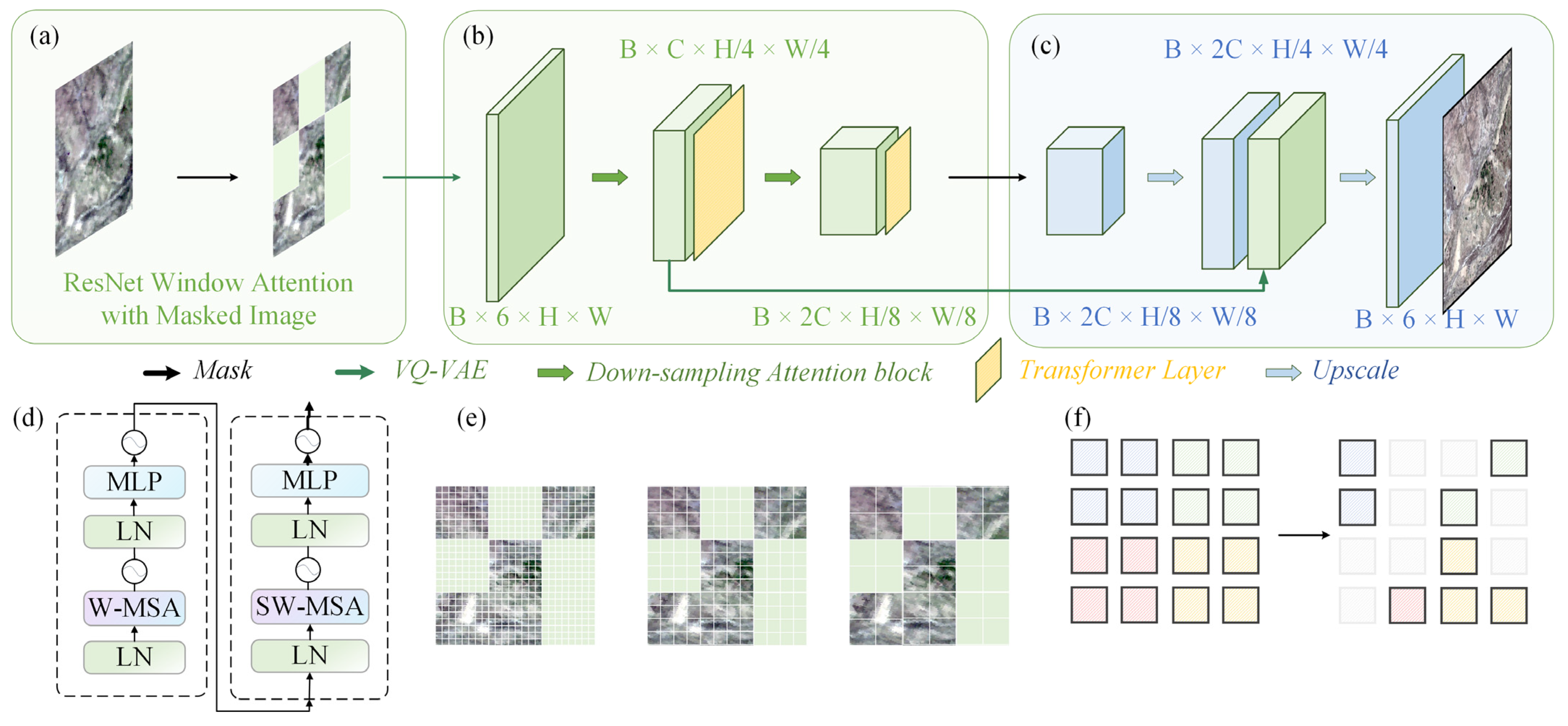
2.2. Model Design
2.3. Training and Evaluation Strategy
3. Results
3.1. Evaluation of Benchmark Dataset
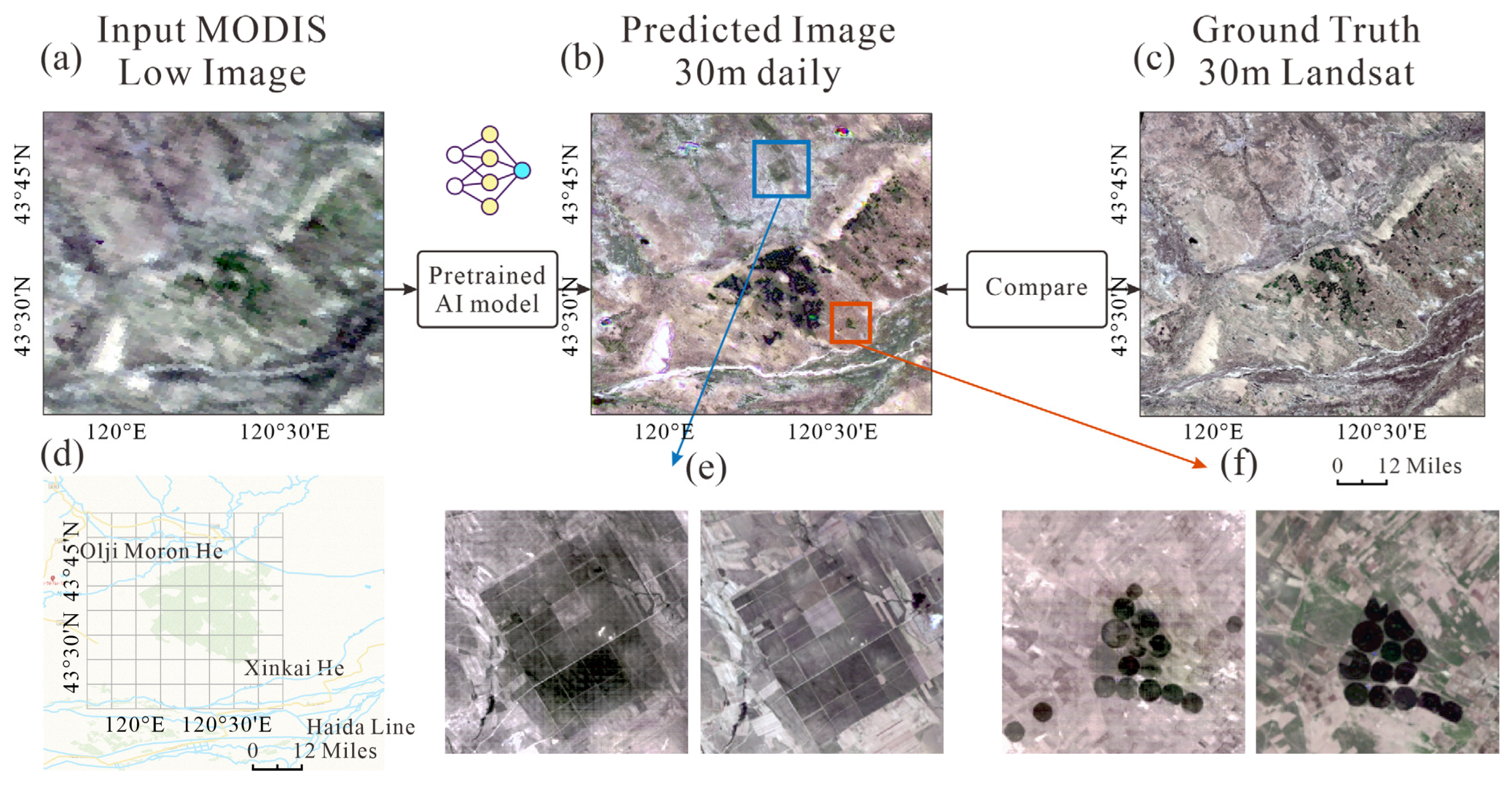
3.2. Spatial Fusion Map
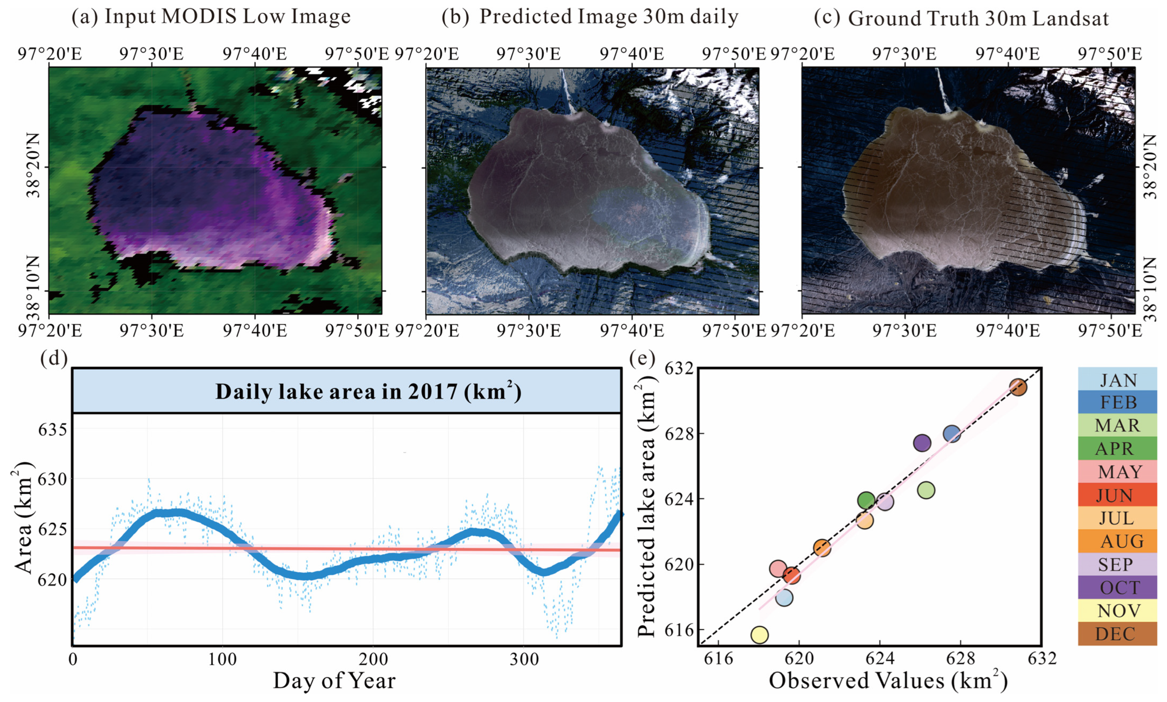
3.3. Application in Lake Area
4. Discussion
4.1. Ablation Studies
4.2. Comparison with SDC Products
4.3. Challenges in Handling Lake Boundaries with Mixed Pixels
4.4. Application in Other Regions and Data Fusion
5. Conclusions
Supplementary Materials
Author Contributions
Funding
Data Availability Statement
Acknowledgments
Conflicts of Interest
Abbreviations
| STF | Spatiotemporal fusion |
| DL | Deep learning |
| MAE | Masked Autoencoders |
| VQ-VAE | Vector Quantized Variational Autoencoder |
References
- Liu, Y.; Yang, J.; Chen, Y.; Fang, G.; Li, W. The temporal and spatial variations in lake surface areas in Xinjiang, China. Water 2018, 10, 431. [Google Scholar] [CrossRef]
- Huang, Z.; Xu, J.; Zheng, L. Long-Term Change of Lake Water Storage and Its Response to Climate Change for Typical Lakes in Arid Xinjiang, China. Water 2023, 15, 1444. [Google Scholar] [CrossRef]
- Yamazaki, D.; Trigg, M.A.; Ikeshima, D. Development of a global ~90m water body map using multi-temporal Landsat images. Remote Sens. Environ. 2015, 171, 337–351. [Google Scholar] [CrossRef]
- Yao, F.; Livneh, B.; Rajagopalan, B.; Wang, J.; Crétaux, J.-F.; Wada, Y.; Berge-Nguyen, M. Satellites reveal widespread decline in global lake water storage. Science 2023, 380, 743–749. [Google Scholar] [CrossRef]
- Wang, Z.; Liu, X.; Li, W.; He, S.; Zheng, T. Temporal and Spatial Variation Analysis of Lake Area Based on the ESTARFM Model: A Case Study of Qilu Lake in Yunnan Province, China. Water 2023, 15, 1800. [Google Scholar] [CrossRef]
- Wang, Y.; Dong, L.n.; Wang, L.; Jin, J. Satellite Reveals a Coupling between Forest Displacement and Landscape Fragmentation across the Economic Corridor of the Eurasia Continent. Forests 2024, 15, 1768. [Google Scholar] [CrossRef]
- Feng, G.; Masek, J.; Schwaller, M.; Hall, F. On the blending of the Landsat and MODIS surface reflectance: Predicting daily Landsat surface reflectance. IEEE Trans. Geosci. Remote Sens. 2006, 44, 2207–2218. [Google Scholar] [CrossRef]
- Roy, D.P.; Wulder, M.A.; Loveland, T.R.; Woodcock, C.E.; Allen, R.G.; Anderson, M.C.; Helder, D.; Irons, J.R.; Johnson, D.M.; Kennedy, R.; et al. Landsat-8: Science and product vision for terrestrial global change research. Remote Sens. Environ. 2014, 145, 154–172. [Google Scholar] [CrossRef]
- Sun, C.; Li, J.; Liu, Y.; Pan, T.; Shi, K.; Cai, X. Synthesizing Landsat images using time series model-fitting methods for China’s coastal areas against sparse and irregular observations. GIScience Remote Sens. 2024, 61, 2421574. [Google Scholar] [CrossRef]
- Malenovský, Z.; Bartholomeus, H.M.; Acerbi-Junior, F.W.; Schopfer, J.T.; Painter, T.H.; Epema, G.F.; Bregt, A.K. Scaling dimensions in spectroscopy of soil and vegetation. Int. J. Appl. Earth Obs. Geoinf. 2007, 9, 137–164. [Google Scholar] [CrossRef]
- Acerbi-Junior, F.W.; Clevers, J.G.P.W.; Schaepman, M.E. The assessment of multi-sensor image fusion using wavelet transforms for mapping the Brazilian Savanna. Int. J. Appl. Earth Obs. Geoinf. 2006, 8, 278–288. [Google Scholar] [CrossRef]
- Gevaert, C.M.; García-Haro, F.J. A comparison of STARFM and an unmixing-based algorithm for Landsat and MODIS data fusion. Remote Sens. Environ. 2015, 156, 34–44. [Google Scholar] [CrossRef]
- Huang, B.; Song, H. Spatiotemporal Reflectance Fusion via Sparse Representation. IEEE Trans. Geosci. Remote Sens. 2012, 50, 3707–3716. [Google Scholar] [CrossRef]
- Wei, Q.; Bioucas-Dias, J.; Dobigeon, N.; Tourneret, J.Y. Hyperspectral and Multispectral Image Fusion Based on a Sparse Representation. IEEE Trans. Geosci. Remote Sens. 2015, 53, 3658–3668. [Google Scholar] [CrossRef]
- Moosavi, V.; Talebi, A.; Mokhtari, M.H.; Shamsi, S.R.F.; Niazi, Y. A wavelet-artificial intelligence fusion approach (WAIFA) for blending Landsat and MODIS surface temperature. Remote Sens. Environ. 2015, 169, 243–254. [Google Scholar] [CrossRef]
- Chen, B.; Chen, L.; Huang, B.; Michishita, R.; Xu, B. Dynamic monitoring of the Poyang Lake wetland by integrating Landsat and MODIS observations. ISPRS J. Photogramm. Remote Sens. 2018, 139, 75–87. [Google Scholar] [CrossRef]
- Dao, P.D.; Mong, N.T.; Chan, H.-P. Landsat-MODIS image fusion and object-based image analysis for observing flood inundation in a heterogeneous vegetated scene. GISci. Remote Sens. 2019, 56, 1148–1169. [Google Scholar] [CrossRef]
- Heimhuber, V.; Tulbure, M.G.; Broich, M. Addressing spatio-temporal resolution constraints in Landsat and MODIS-based mapping of large-scale floodplain inundation dynamics. Remote Sens. Environ. 2018, 211, 307–320. [Google Scholar] [CrossRef]
- Tan, Z.; Wang, X.; Chen, B.; Liu, X.; Zhang, Q. Surface water connectivity of seasonal isolated lakes in a dynamic lake-floodplain system. J. Hydrol. 2019, 579, 124154. [Google Scholar] [CrossRef]
- Zhang, F.; Zhu, X.; Liu, D. Blending MODIS and Landsat images for urban flood mapping. Int. J. Remote Sens. 2014, 35, 3237–3253. [Google Scholar] [CrossRef]
- Sadeh, Y.; Zhu, X.; Dunkerley, D.; Walker, J.P.; Zhang, Y.; Rozenstein, O.; Manivasagam, V.S.; Chenu, K. Fusion of Sentinel-2 and PlanetScope time-series data into daily 3 m surface reflectance and wheat LAI monitoring. Int. J. Appl. Earth Obs. Geoinf. 2021, 96, 102260. [Google Scholar] [CrossRef]
- Emelyanova, I.V.; McVicar, T.R.; Van Niel, T.G.; Li, L.T.; van Dijk, A.I.J.M. Assessing the accuracy of blending Landsat–MODIS surface reflectances in two landscapes with contrasting spatial and temporal dynamics: A framework for algorithm selection. Remote Sens. Environ. 2013, 133, 193–209. [Google Scholar] [CrossRef]
- Li, J.; Li, Y.; He, L.; Chen, J.; Plaza, A. Spatio-temporal fusion for remote sensing data: An overview and new benchmark. Sci. China Inf. Sci. 2020, 63, 140301. [Google Scholar] [CrossRef]
- Hilker, T.; Wulder, M.A.; Coops, N.C.; Linke, J.; McDermid, G.; Masek, J.G.; Gao, F.; White, J.C. A new data fusion model for high spatial- and temporal-resolution mapping of forest disturbance based on Landsat and MODIS. Remote Sens. Environ. 2009, 113, 1613–1627. [Google Scholar] [CrossRef]
- Zhu, X.; Chen, J.; Gao, F.; Chen, X.; Masek, J.G. An enhanced spatial and temporal adaptive reflectance fusion model for complex heterogeneous regions. Remote Sens. Environ. 2010, 114, 2610–2623. [Google Scholar] [CrossRef]
- Li, X.; Ling, F.; Foody, G.M.; Boyd, D.S.; Jiang, L.; Zhang, Y.; Zhou, P.; Wang, Y.; Chen, R.; Du, Y. Monitoring high spatiotemporal water dynamics by fusing MODIS, Landsat, water occurrence data and DEM. Remote Sens. Environ. 2021, 265, 112680. [Google Scholar] [CrossRef]
- Roy, D.P.; Ju, J.; Lewis, P.; Schaaf, C.; Gao, F.; Hansen, M.; Lindquist, E. Multi-temporal MODIS–Landsat data fusion for relative radiometric normalization, gap filling, and prediction of Landsat data. Remote Sens. Environ. 2008, 112, 3112–3130. [Google Scholar] [CrossRef]
- Zhu, X.; Helmer, E.H.; Gao, F.; Liu, D.; Chen, J.; Lefsky, M.A. A flexible spatiotemporal method for fusing satellite images with different resolutions. Remote Sens. Environ. 2016, 172, 165–177. [Google Scholar] [CrossRef]
- Zhao, Y.; Huang, B.; Song, H. A robust adaptive spatial and temporal image fusion model for complex land surface changes. Remote Sens. Environ. 2018, 208, 42–62. [Google Scholar] [CrossRef]
- Zheng, Y.; Song, H.; Sun, L.; Wu, Z.; Jeon, B. Spatiotemporal Fusion of Satellite Images via Very Deep Convolutional Networks. Remote Sens. 2019, 11, 2701. [Google Scholar] [CrossRef]
- Wang, Q.; Tang, Y.; Tong, X.; Atkinson, P.M. Virtual image pair-based spatio-temporal fusion. Remote Sens. Environ. 2020, 249, 112009. [Google Scholar] [CrossRef]
- Luo, Y.; Guan, K.; Peng, J.; Wang, S.; Huang, Y. STAIR 2.0: A Generic and Automatic Algorithm to Fuse Modis, Landsat, and Sentinel-2 to Generate 10 m, Daily, and Cloud-/Gap-Free Surface Reflectance Product. Remote Sens. 2020, 12, 3209. [Google Scholar] [CrossRef]
- Hu, F.; Xia, G.-S.; Hu, J.; Zhang, L. Transferring Deep Convolutional Neural Networks for the Scene Classification of High-Resolution Remote Sensing Imagery. Remote Sens. 2015, 7, 14680–14707. [Google Scholar] [CrossRef]
- Li, M.; Wu, P.; Wang, B.; Park, H.; Yang, H.; Wu, Y. A Deep Learning Method of Water Body Extraction From High Resolution Remote Sensing Images With Multisensors. IEEE J. Sel. Top. Appl. Earth Obs. Remote Sens. 2021, 14, 3120–3132. [Google Scholar] [CrossRef]
- Li, Y.; Dang, B.; Zhang, Y.; Du, Z. Water body classification from high-resolution optical remote sensing imagery: Achievements and perspectives. ISPRS J. Photogramm. Remote Sens. 2022, 187, 306–327. [Google Scholar] [CrossRef]
- Han, W.; Zhang, X.; Wang, Y.; Wang, L.; Huang, X.; Li, J.; Wang, S.; Chen, W.; Li, X.; Feng, R.; et al. A survey of machine learning and deep learning in remote sensing of geological environment: Challenges, advances, and opportunities. ISPRS J. Photogramm. Remote Sens. 2023, 202, 87–113. [Google Scholar] [CrossRef]
- Wang, L.; Wu, J.; Li, R.; Song, Y.; Zhou, J.; Rui, X.; Xu, H. A Weight Assignment Algorithm for Incomplete Traffic Information Road Based on Fuzzy Random Forest Method. Symmetry 2021, 13, 1588. [Google Scholar] [CrossRef]
- Liu, Q.; Meng, X.; Li, X.; Shao, F. Detail Injection-Based Spatio-Temporal Fusion for Remote Sensing Images With Land Cover Changes. IEEE Trans. Geosci. Remote Sens. 2023, 61, 5401514. [Google Scholar] [CrossRef]
- Zhang, H.; Song, Y.; Han, C.; Zhang, L. Remote Sensing Image Spatiotemporal Fusion Using a Generative Adversarial Network. IEEE Trans. Geosci. Remote Sens. 2021, 59, 4273–4286. [Google Scholar] [CrossRef]
- Liu, Z.; Lin, Y.; Cao, Y.; Hu, H.; Wei, Y.; Zhang, Z.; Lin, S.; Guo, B. Swin transformer: Hierarchical vision transformer using shifted windows. In Proceedings of the IEEE/CVF International Conference on Computer Vision, Virtual, 11–17 October 2021; pp. 10012–10022. [Google Scholar]
- Wang, L.; Zhang, X.; Leung, L.R.; Chiew, F.H.; AghaKouchak, A.; Ying, K.; Zhang, Y. CAS-Canglong: A skillful 3D Transformer model for sub-seasonal to seasonal global sea surface temperature prediction. arXiv 2024. [Google Scholar] [CrossRef]
- Wang, L.; Zhang, Y. Filling GRACE data gap using an innovative transformer-based deep learning approach. Remote Sens. Environ. 2024, 315, 114465. [Google Scholar] [CrossRef]
- Song, H.; Liu, Q.; Wang, G.; Hang, R.; Huang, B. Spatiotemporal Satellite Image Fusion Using Deep Convolutional Neural Networks. IEEE J. Sel. Top. Appl. Earth Obs. Remote Sens. 2018, 11, 821–829. [Google Scholar] [CrossRef]
- Tan, Z.; Yue, P.; Di, L.; Tang, J. Deriving High Spatiotemporal Remote Sensing Images Using Deep Convolutional Network. Remote Sens. 2018, 10, 1066. [Google Scholar] [CrossRef]
- Tan, Z.; Di, L.; Zhang, M.; Guo, L.; Gao, M. An Enhanced Deep Convolutional Model for Spatiotemporal Image Fusion. Remote Sens. 2019, 11, 2898. [Google Scholar] [CrossRef]
- Liu, X.; Deng, C.; Chanussot, J.; Hong, D.; Zhao, B. StfNet: A Two-Stream Convolutional Neural Network for Spatiotemporal Image Fusion. IEEE Trans. Geosci. Remote Sens. 2019, 57, 6552–6564. [Google Scholar] [CrossRef]
- Yin, Z.; Wu, P.; Foody, G.M.; Wu, Y.; Liu, Z.; Du, Y.; Ling, F. Spatiotemporal Fusion of Land Surface Temperature Based on a Convolutional Neural Network. IEEE Trans. Geosci. Remote Sens. 2021, 59, 1808–1822. [Google Scholar] [CrossRef]
- Chen, Y.; Shi, K.; Ge, Y.; Zhou, Y. Spatiotemporal Remote Sensing Image Fusion Using Multiscale Two-Stream Convolutional Neural Networks. IEEE Trans. Geosci. Remote Sens. 2022, 60, 4402112. [Google Scholar] [CrossRef]
- Ran, Q.; Wang, Q.; Zheng, K.; Li, J. Multiscale Attention Spatiotemporal Fusion Model Based on Pyramidal Network Constraints. IEEE Geosci. Remote Sens. Lett. 2024, 21, 5004305. [Google Scholar] [CrossRef]
- Shang, C.; Li, X.; Yin, Z.; Li, X.; Wang, L.; Zhang, Y.; Du, Y.; Ling, F. Spatiotemporal Reflectance Fusion Using a Generative Adversarial Network. IEEE Trans. Geosci. Remote Sens. 2022, 60, 5400915. [Google Scholar] [CrossRef]
- Liu, Q.; Meng, X.; Shao, F.; Li, S. PSTAF-GAN: Progressive Spatio-Temporal Attention Fusion Method Based on Generative Adversarial Network. IEEE Trans. Geosci. Remote Sens. 2022, 60, 5408513. [Google Scholar] [CrossRef]
- Filali Boubrahimi, S.; Neema, A.; Nassar, A.; Hosseinzadeh, P.; Hamdi, S.M. Spatiotemporal Data Augmentation of MODIS-Landsat Water Bodies Using Adversarial Networks. Water Resour. Res. 2024, 60, e2023WR036342. [Google Scholar] [CrossRef]
- Meng, X.; Wang, N.; Shao, F.; Li, S. Vision Transformer for Pansharpening. IEEE Trans. Geosci. Remote Sens. 2022, 60, 5409011. [Google Scholar] [CrossRef]
- Li, X.; Li, Y.; Chen, H.; Sun, J.; Wang, M.; Chen, L. WTFusion: Wavelet-Assisted Transformer Network for Multisensor Image Fusion. IEEE Sens. J. 2024, 24, 37152–37168. [Google Scholar] [CrossRef]
- Chen, G.; Jiao, P.; Hu, Q.; Xiao, L.; Ye, Z. SwinSTFM: Remote Sensing Spatiotemporal Fusion Using Swin Transformer. IEEE Trans. Geosci. Remote Sens. 2022, 60, 5410618. [Google Scholar] [CrossRef]
- Luo, X.; Fu, G.; Yang, J.; Cao, Y.; Cao, Y. Multi-Modal Image Fusion via Deep Laplacian Pyramid Hybrid Network. IEEE Trans. Circuits Syst. Video Technol. 2023, 33, 7354–7369. [Google Scholar] [CrossRef]
- Zhao, Y.; Zheng, Q.; Zhu, P.; Zhang, X.; Ma, W. TUFusion: A Transformer-Based Universal Fusion Algorithm for Multimodal Images. IEEE Trans. Circuits Syst. Video Technol. 2024, 34, 1712–1725. [Google Scholar] [CrossRef]
- Zhang, X.; Wang, X.; Yan, C.; Sun, Q. EV-Fusion: A Novel Infrared and Low-Light Color Visible Image Fusion Network Integrating Unsupervised Visible Image Enhancement. IEEE Sens. J. 2024, 24, 4920–4934. [Google Scholar] [CrossRef]
- He, K.; Zhang, X.; Ren, S.; Sun, J. Deep Residual Learning for Image Recognition. In Proceedings of the 2016 IEEE Conference on Computer Vision and Pattern Recognition (CVPR), Las Vegas, NV, USA, 27–30 June 2016; pp. 770–778. [Google Scholar]
- Yang, J.; Wright, J.; Huang, T.S.; Ma, Y. Image Super-Resolution Via Sparse Representation. IEEE Trans. Image Process. 2010, 19, 2861–2873. [Google Scholar] [CrossRef]
- Vaswani, A.; Shazeer, N.; Parmar, N.; Uszkoreit, J.; Jones, L.; Gomez, A.N.; Kaiser, Ł.; Polosukhin, I. Attention is all you need. In Proceedings of the 31st International Conference on Neural Information Processing Systems, Long Beach, CA, USA, 4–9 December 2017; pp. 6000–6010. [Google Scholar]
- Liang, J.; Cao, J.; Sun, G.; Zhang, K.; Gool, L.V.; Timofte, R. SwinIR: Image Restoration Using Swin Transformer. In Proceedings of the 2021 IEEE/CVF International Conference on Computer Vision Workshops (ICCVW), Montreal, BC, Canada, 11–17 October 2021; pp. 1833–1844. [Google Scholar]
- Ledig, C.; Theis, L.; Huszár, F.; Caballero, J.; Cunningham, A.; Acosta, A.; Aitken, A.; Tejani, A.; Totz, J.; Wang, Z.; et al. Photo-Realistic Single Image Super-Resolution Using a Generative Adversarial Network. In Proceedings of the 2017 IEEE Conference on Computer Vision and Pattern Recognition (CVPR), Honolulu, HI, USA, 21–26 July 2017; pp. 105–114. [Google Scholar]
- Isono, R.; Naganuma, K.; Ono, S. Robust Spatiotemporal Fusion of Satellite Images: A Constrained Convex Optimization Approach. IEEE Trans. Geosci. Remote Sens. 2024, 62, 5404516. [Google Scholar] [CrossRef]
- Chen, S.; Wang, J.; Gong, P. ROBOT: A spatiotemporal fusion model toward seamless data cube for global remote sensing applications. Remote Sens. Environ. 2023, 294, 113616. [Google Scholar] [CrossRef]
- Chen, S.; Wang, J.; Liu, Q.; Liang, X.; Liu, R.; Qin, P.; Yuan, J.; Wei, J.; Yuan, S.; Huang, H.; et al. Global 30 m seamless data cube (2000–2022) of land surface reflectance generated from Landsat 5, 7, 8, and 9 and MODIS Terra constellations. Earth Syst. Sci. Data 2024, 16, 5449–5475. [Google Scholar] [CrossRef]


| Name | Type | Target Resolution | Spatial Interpolation | Temporal Gap Filling | Input Data (Revisit Frequency) | Reference |
|---|---|---|---|---|---|---|
| STARFM | Weight function-based method | 30 m; daily | N/A | √ | MODIS (MOD09GHK; daily), Landsat (Landsat-7ETM+; 16 days) | [7] |
| Semi-physical model | Semi-physical fusion approach | 30 m; daily | √ | N/A | MODIS (MODIS BRDF/Albedo; 16 days), Landsat (Landsat ETM+ L1G; 16 days) | [27] |
| STAARCH | Hybrid method (weight function-based and unmixing method) | 30 m; 8 days | N/A | √ | MODIS (MOD09/MYD09; 8 days), Landsat (Landsat ETM; 16 days) | [24] |
| ESTARFM | Weight function-based method | 30 m; daily | √ | N/A | MODIS (MOD09GQ; daily), Landsat (Landsat 8 OLI C1 Level 2; 16 days) | [25] |
| STRUM | Hybrid method (weight function-based and unmixing method) | 30 m; daily | √ | N/A | MODIS (MODIS MCD43A4 BRDF; 8 days), Landsat (Landsat 8 OLI; 8 days) | [12] |
| FSDAF | Hybrid method (weight function-based and unmixing method) | 30 m | √ | N/A | MODIS (MOD09GA Collection 5; daily), Landsat (Landsat 7 ETM+; 16 days) | [28] |
| RASTFM | Weight function-based method | 30 m | √ | √ | MODIS (MOD09; 8 days), Landsat (Landsat-7; 16 days) | [29] |
| VDCNSTF | Deep learning-based method | 30 m | √ | √ | MODIS (MOD09GA Collection 5; daily), Landsat (Landsat-5 TM; 16 days) | [30] |
| VIPSTF | Hybrid method (weight function-based and unmixing method) | 30 m | √ | √ | MODIS (MOD09GA Collection 5; daily), Landsat (Landsat 7 ETM+; 16 days) | [31] |
| STAIR | Weight function-based method | 30 m | √ | √ | MODIS (MCD43A4; daily), Landsat (Landsat 7 and 8 Level 2; 16 days) | [32] |
| STSWM | Hybrid method (weight function-based and unmixing method) | 30 m; 8 days | N/A | N/A | MODIS (MOD09A1; 8 days), Landsat (Landsat 7 and 8 Level 2; 16 days) | [26] |
| MosaicFormer | Masked Autoencoders with the Swin Transformer architecture | 30 m; daily | √ | √ | MODIS (MOD09GA Collection 5; daily); Landsat (Landsat 8 OLI; 8 days) | This study |
| Dataset | Image Size | Data Pairs | Timespan | Description |
|---|---|---|---|---|
| Benchmark | 2480 × 2800 × 6 | 27 | 30 May 2013 to 6 December 2018 | Rural areas for model evaluation |
| Lake | 2000 × 1200 × 6 | 12 | 1 January 2017 to 31 December 2017 | A lake for model application |
Disclaimer/Publisher’s Note: The statements, opinions and data contained in all publications are solely those of the individual author(s) and contributor(s) and not of MDPI and/or the editor(s). MDPI and/or the editor(s) disclaim responsibility for any injury to people or property resulting from any ideas, methods, instructions or products referred to in the content. |
© 2025 by the authors. Licensee MDPI, Basel, Switzerland. This article is an open access article distributed under the terms and conditions of the Creative Commons Attribution (CC BY) license (https://creativecommons.org/licenses/by/4.0/).
Share and Cite
Zheng, D.; Lv, A. MosaicFormer: A Novel Approach to Remote Sensing Spatiotemporal Data Fusion for Lake Water Monitors. Remote Sens. 2025, 17, 1138. https://doi.org/10.3390/rs17071138
Zheng D, Lv A. MosaicFormer: A Novel Approach to Remote Sensing Spatiotemporal Data Fusion for Lake Water Monitors. Remote Sensing. 2025; 17(7):1138. https://doi.org/10.3390/rs17071138
Chicago/Turabian StyleZheng, Dongxue, and Aifeng Lv. 2025. "MosaicFormer: A Novel Approach to Remote Sensing Spatiotemporal Data Fusion for Lake Water Monitors" Remote Sensing 17, no. 7: 1138. https://doi.org/10.3390/rs17071138
APA StyleZheng, D., & Lv, A. (2025). MosaicFormer: A Novel Approach to Remote Sensing Spatiotemporal Data Fusion for Lake Water Monitors. Remote Sensing, 17(7), 1138. https://doi.org/10.3390/rs17071138