Toward Robust GNSS Real-Time Orbit Determination for Microsatellites Using Factor Graph Optimization

Abstract

Extended Kalman Filter (EKF) is extensively employed in Global Navigation Satellite System (GNSS)-based real-time orbit determination (RTOD) for microsatellites due to its low complexity. However, the performance of EKF-RTOD is markedly degraded when the microsatellite deviates from a stable Earth-pointing attitude and employs a low-cost receiver. Factor graph optimization (FGO), which addresses nonlinear problems through multiple iterations and re-linearization, has demonstrated superior accuracy and robustness compared to EKF in challenging environments such as urban canyons. In this study, we introduce a novel FGO-based RTOD (FGO-RTOD) approach, which integrates state transfer factors to establish temporal connections between state nodes across multiple epochs. Real-time processing is achieved through a sliding window mechanism combined with marginalization. This paper evaluates the performance of the proposed algorithm in a regular scenario using data from GRACE-FO-A, which maintains the Earth-pointing attitude and employs a high-performance receiver. The positioning results of GRACE-FO-A indicate that FGO-RTOD marginally outperforms EKF-RTOD in accuracy. Furthermore, the performance of FGO-RTOD is assessed in challenging scenarios using simulation data and on-orbit data from Tianping-2B microsatellite, which is not in an Earth-pointing attitude and employs a low-cost receiver. The simulation results reveal that FGO-RTOD reduces the Root Mean Square (RMS) of positioning error by 79.0% relative to EKF-RTOD and exhibits significantly enhanced smoothing. In the Tianping-2B experiments, FGO-RTOD reduces the RMS of carrier-phase ionosphere-free combination residuals from 2 cm to 1 cm relative to EKF-RTOD, alongside a substantial improvement in the ratio of valid observations. These findings underscore the effectiveness of FGO-RTOD in managing outlier measurements in challenging scenarios.

1. Introduction

Microsatellites have experienced rapid development in recent years, driven by their cost-effectiveness and short manufacturing cycles [1,2,3]. As a fundamental prerequisite for satellites to execute diverse tasks, satellite navigation technology has been extensively investigated, with the Global Navigation Satellite System (GNSS) emerging as the predominant method due to its exceptional stability and precision. Extended Kalman Filter (EKF) plays a crucial role in real-time orbit determination (RTOD) to acquire accurate position and velocity information by utilizing broadcast ephemeris, pseudorange, and carrier phase observations obtained from spaceborne GNSS receivers. Under regular conditions, EKF-RTOD can achieve dm-level accuracy when the satellite maintains a stable Earth-pointing attitude and employs a high-precision receiver [4,5]. However, the performance of EKF-RTOD is often compromised when processing low-quality observations from low-cost spaceborne receivers on microsatellites. Moreover, attitude maneuvers are inevitable for microsatellites when executing specific tasks, which also leads to degradation of the quality of GNSS observations. The above adverse factors make it too challenging for EKF-RTOD to achieve robust and accurate orbit determination in microsatellites.

Factor graph optimization (FGO) has gained popularity in the field of simultaneous localization and mapping (SLAM) due to its flexibility [6,7,8]. In a factor graph framework, the measurements of sensors are encoded as factor nodes that are simply added to the framework when measurements are generated. FGO is capable of handling nonlinear optimization problems through iterative re-linearization and can also leverage the correlation among historical epochs to obtain a globally optimal estimation [9,10]. Moreover, FGO can use a loss function to robustly handle outlier measurements [11,12]. Based on these properties, FGO tends to yield smoother and more accurate results compared to traditional filter-based methods. Therefore, in recent years, researchers have begun to attempt to apply FGO to GNSS to study its robust positioning performance in challenging environments. Sünderhauf and Protzel [13] were the first to use FGO for GNSS positioning. They focused on pseudorange measurements and treated observations affected by multipath errors as outliers in the optimization problem. Watson and Gross [14] proposed an FGO-based precise point positioning (PPP) framework for GNSS with real-time optimization using incremental smoothing and mapping. Their validation dataset showed that FGO-based PPP demonstrated better convergence performance compared to EKF-based PPP. Wen and Hsu [15] developed an FGO-based GNSS real-time kinematic (RTK) framework and investigated the time correlation of pseudorange, carrier phase, and Doppler measurements. They verified its localization performance in challenging urban canyons of Hong Kong where FGO-RTK outperformed EKF-RTK. Wen et al. [12] proposed a graduated non-convexity FGO method to mitigate the effect of GNSS outliers by estimating the optimal weights of GNSS measurements. Bai et al. [11] used carrier phase measurements within a window to constrain the states in the factor graph and compared the effectiveness of Huber and Cauchy loss functions in suppressing outlier measurements. Wang et al. [9] obtained results that FGO-RTK was superior to EKF-RTK in moderately and highly complex urban environments using a marginalization-based carrier phase ambiguity propagation method. Xin et al. [16] proposed a sliding window-based FGO to meet the real-time requirement. They experimented in the complex urban canyon of Hong Kong using a low-cost GNSS receiver and finally achieved real-time results with m-level average horizontal positioning error.

For low Earth orbit (LEO) satellites, the absence of external control forces allows for a precise characterization of inter-epoch motion by modeling the forces acting on the satellite. This renders FGO a promising approach for implementing RTOD. Low-cost receivers are ideal for deployment on microsatellites due to their minimal power consumption and compact size. However, these receivers often suffer from relatively unstable clock sources and suboptimal signal quality. When microsatellites are in non-Earth-pointing attitudes, signals from GNSS satellites with low or even negative elevation angles are susceptible to interference from atmospheric delays and severe multipath effects, which result in degradation of the quality of the observations. What’s worse, the number of observable satellites will also decrease significantly, leading to an increase in the Geometry Dilution of Precision (GDOP). When FGO is used, data correlations are taken into account from multiple epochs simultaneously and the states are refined through multiple iterations. Therefore, FGO can resist the degradation of observed signal quality or unreasonable fluctuation of states among epochs to obtain the globally optimal solution. The above advantages give FGO the opportunity to provide robust and high-precision RTOD for microsatellites in challenging environments. Nevertheless, the real-time processing capability of factor graph optimization remains underexplored, with most research focusing on optimization using progressively expanding windows, which inevitably escalates computational demands.

To address these challenges, this paper proposes a factor graph optimization framework based on a sliding window for RTOD, and the main contributions of this paper include:

• To the best of the authors’ knowledge, this paper is the first to use sliding window-based FGO for RTOD, and we propose state transfer factors, including dynamics factor, clock offset variation factor, and ambiguity variation factor, to enhance the connection between multiple epochs;
• We provide a detailed procedure for applying Schur complement-based marginalization to sliding window-based FGO, which explicitly incorporates Jacobian matrices and covariance to ensure accurate uncertainty propagation, and clearly defines the state nodes affected by marginalization. The marginalization significantly enhances computational efficiency without compromising accuracy;
• We processed the first published data of the GNSS receiver on the Tianping-2B microsatellite and showed that the FGO-based RTOD solution exhibits superior robustness compared to EKF-RTOD.

2. Construction of Factor Graph Optimization

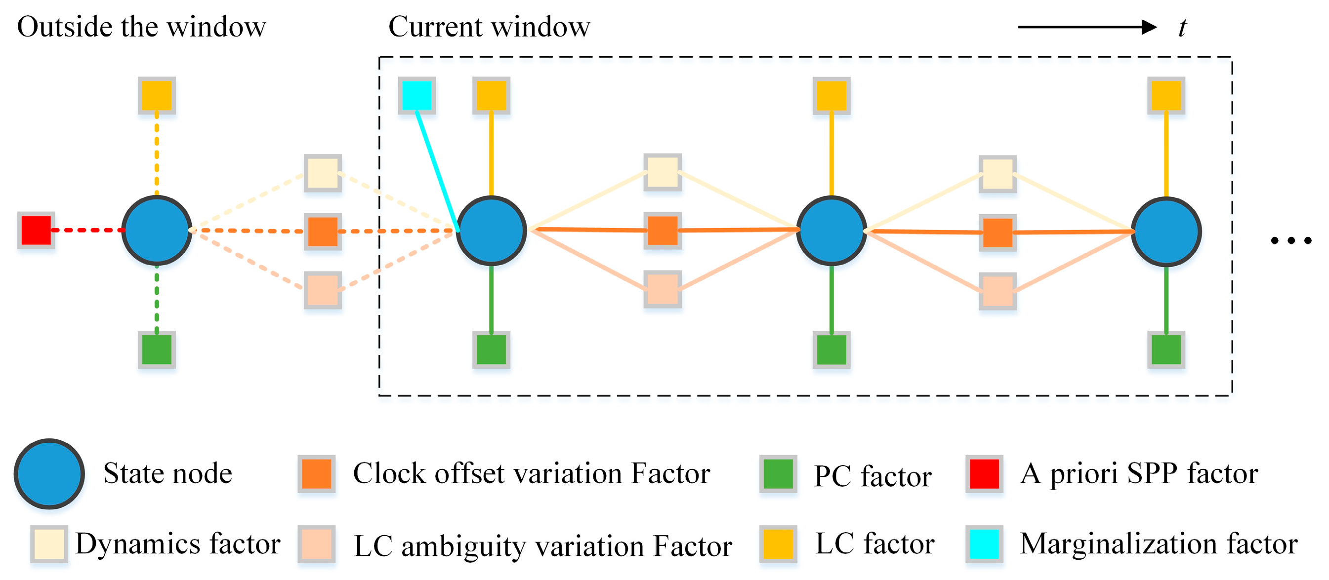
The basic design of the FGO-based RTOD (FGO-RTOD) proposed in this paper is shown in Figure 1. The circles denote the state nodes. In order to meet the requirements of real-time applications, we designed the factor graph based on a sliding window. The real-time solution of FGO-RTOD is obtained from the latest epoch in the window. RTOD in this paper is implemented using the ionosphere-free combined measurements of the code and phase recorded as PC and LC [17,18]. The set of states $\chi$ of the GNSS receiver in the sliding window is represented as follows:

$$\begin{array}{l}\chi =\left[x\left(k-n+1\right);\dots ,x\left(k-1\right);x\left(k\right);p\right]\\ x\left(k\right)=\left[y\left(k\right);\delta t_r\left(k\right);N_{12}\left(k\right)\right]\end{array}$$

(1)

where n denotes the length of the sliding window, $p=\left[C_D;C_R\right]$ is the dynamic parameter vector that includes drag coefficient $C_D$ and solar radiation pressure coefficient $C_R$. $x\left(k\right)$ denotes the state at epoch k which involves the position and velocity state vector $y\left(k\right)$, receiver clock offset $\delta t_r\left(k\right)$, and LC ambiguity vector $N_{12}\left(k\right)$ of received GNSS satellites. All factors in Figure 1 will be presented later.

2.1. Measurement Factors

For a spaceborne receiver on a LEO satellite, the undifferenced and uncombined (UDUC) observation models of pseudorange P and carrier phase L are formulated as:

$$\begin{array}{l}{P}_f^s={\rho }^s+c(\delta t_r-\delta t^s)+I_f^s+{\epsilon }_{P_f}^s\\ L_f^s={\rho }^s+c(\delta t_r-\delta t^s)+{\lambda }_f{N}_f^s-I_f^s+{\epsilon }_{L_f}^s\end{array}$$

(2)

where ${\rho }^s$ represents the geometric range between the GNSS satellite (superscript s) and the receiver; c is the speed of light; δt^s and δt_r are the clock offsets of the GNSS satellite and receiver, respectively; $I_f^s$ represents the ionospheric path delay, f and λ are the frequency and wavelength of the carrier, respectively; $N_f^s$ is the carrier phase ambiguity; ${\epsilon }_{P_f}^s$ and ${\epsilon }_{L_f}^s$ denote the pseudorange and carrier phase observation noises. Note that most signals from high-elevation GPS satellites are not affected by tropospheric delays due to the fact that LEO satellites operate above the troposphere, and we consider possible tropospheric delays for signals from low-elevation GPS satellites as part of the observation noise. All other error terms, such as hardware delays from both the receiver and GNSS satellite, systematic error, multipath, and polarization-induced windup for carrier phase, are enclosed into the ε term [19].

The PC and LC are obtained using dual-frequency ionosphere-free combination, as shown in Equations (3) and (4), respectively:

$$P_{12}^s={\rho }^s+c\left(\delta t_r-\delta t^s\right)+{\epsilon }_{P_{12}}^s$$

(3)

$$L_{12}^s={\rho }^s+c\left(\delta t_r-\delta t^s\right)+{\lambda }_{12}{N}_{12}^s+{\epsilon }_{L_{12}}^s$$

(4)

where ${\lambda }_{12}{N}_{12}^s={\displaystyle \frac{f_1^2}{f_1^2-f_2^2}}{\lambda }_1{N}_1^s-{\displaystyle \frac{f_2^2}{f_1^2-f_2^2}}{\lambda }_2{N}_2^s$.

The error function of PC and LC at epoch k can be denoted as $e_{P,12}^s\left(k\right)$ and $e_{L,12}^s\left(k\right)$:

$$\begin{array}{l}{‖e_{P,12}^s\left(k\right)‖}_{R_{P,12}^s(k)}^2={‖P_{12}^s\left(k\right)-\left({\rho }^s\left(k\right)+c\left(\delta t_r\left(k\right)-\delta t^s\left(k\right)\right)\right)‖}_{R_{P,12}^s(k)}^2\\ {‖e_{L,12}^s\left(k\right)‖}_{R_{L,12}^s\left(k\right)}^2={‖L_{12}^s\left(k\right)-\left({\rho }^s\left(k\right)+c\left(\delta t_r\left(k\right)-\delta t^s\left(k\right)\right)+{\lambda }_{12}{N}_{12}^s\left(t\right)\right)‖}_{R_{L,12}^s\left(k\right)}^2\end{array}$$

(5)

where ${‖e‖}_{\Omega }^2=e^T{\Omega }^{-1}e$ is defined as the squared Mahalanobis distance [8] for the covariance matrix $\Omega$. $R_{P,12}^s$ and $R_{L,12}^s$ are the variances of PC and LC, which can be propagated from the UDUC pseudorange variance ${\left({\sigma }_P^s\right)}^2$ and carrier-phase variance ${\left({\sigma }_L^s\right)}^2$ through the error propagation law, respectively. ${\sigma }_P^s$ and ${\sigma }_L^s$ are set to 0.3 and 0.003, respectively.

The measurement factor ${‖e_z\left(k\right)‖}_{R(k)}^2$ of epoch k consists of the sets of LC and PC factors for all observed satellites $s\in [1,m_k]$:

$$e_z\left(k\right)={\left[e_{P,12}^1\left(k\right),e_{L,12}^1\left(k\right),\cdots ,e_{P,12}^{m_k}\left(k\right),e_{L,12}^{m_k}\left(k\right)\right]}^T$$

(6)

$$R(k)=diag\left\{R_{P,12}^1\left(k\right),R_{L,12}^1\left(k\right),\cdots ,R_{P,12}^{m_k}\left(k\right),R_{L,12}^{m_k}\left(k\right)\right\}$$

(7)

2.2. State Transfer Factor

In order to better establish the relationship between state nodes within a window, a state transfer factor is proposed in this paper. The state transfer factor ${‖e_f\left(k\right)‖}_{Q(k)}^2$ at epoch $k\ge 1$ consists of three components: the dynamics factor $e_D\left(k\right)$, the clock variation factor $e_C\left(k\right)$, and the LC ambiguity variation factor $e_{N,12}^s\left(k\right)$:

$$e_f\left(k\right)={\left[e_D^T\left(k\right),e_C\left(k\right),e_{N,12}^1\left(k\right),\cdots ,e_{N,12}^{m_k}\left(k\right)\right]}^T$$

(8)

$$Q(k)=diag\left\{Q_D,Q_C,Q_{N,12}^1,\cdots ,Q_{N,12}^{m_k}\right\}$$

(9)

where $Q(k)$ is the process noise matrix. The individual terms in the equations are described in later subsections.

2.2.1. Dynamics Factor

Dynamic force models are used to accurately propagate the satellite state vector over time by means of numerical integration of the first order differential equation [20]:

$$\begin{array}{l}{\displaystyle \frac{\mathrm{d}}{\mathrm{d}t}}y(t_k)=f\left(t_k,y(t_k),p\right)=\left(\begin{array}{c}v(t_k)\\ a\left(t_k,r(t_k),v(t_k),p\right)\end{array}\right)\\ y(k)=y\left(k-1\right)+{\displaystyle {\int }_{t_{k-1}}^{t_k}f}\left(t,y\left(t\right),p\right)\mathrm{d}t+{\epsilon }_D\end{array}$$

(10)

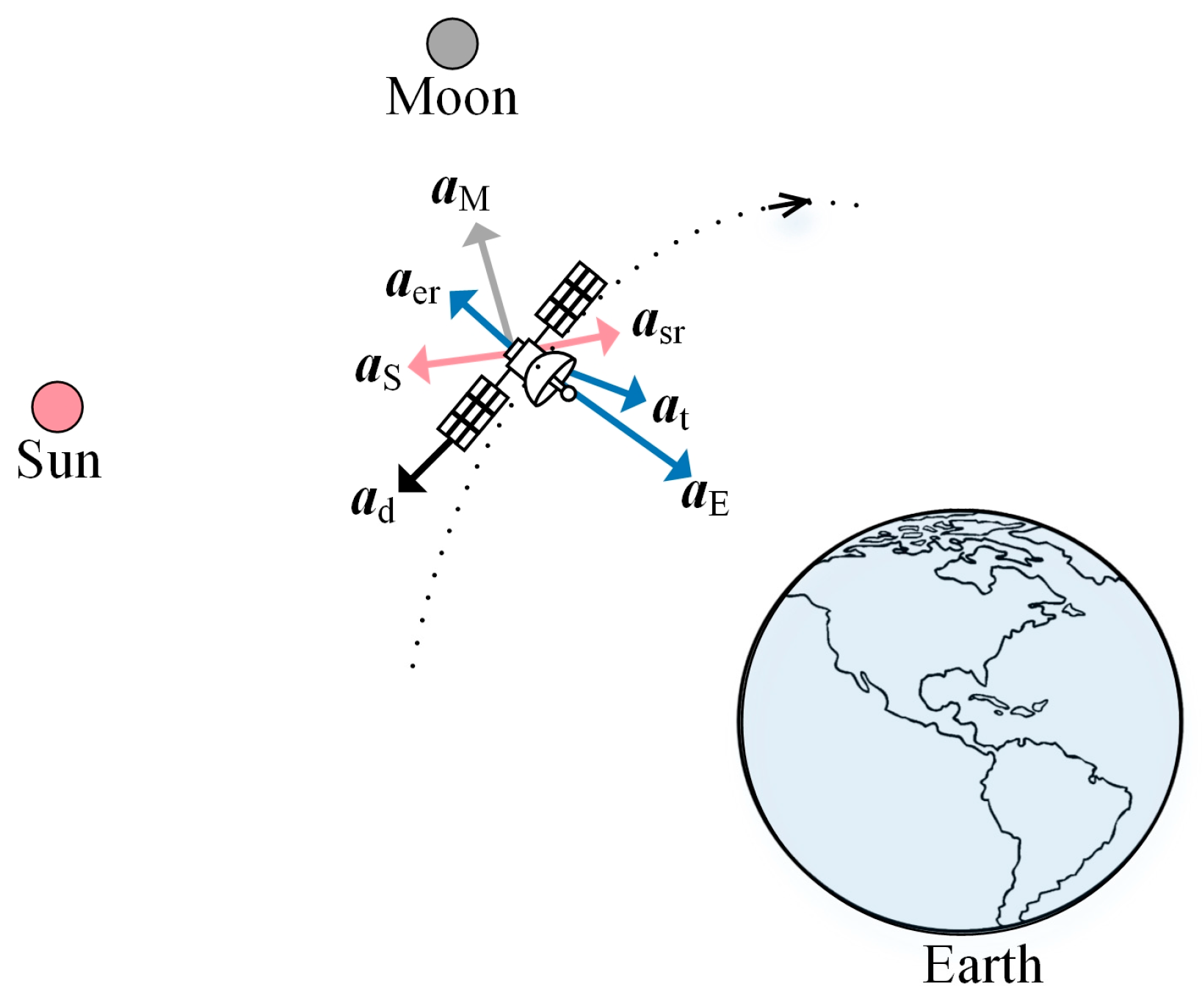
Where $y(t_k)$ is the state vector at $t_k$ includes satellite position $r(t_k)$ and velocity $v(t_k)$, a is the acceleration vector of the satellite in the geocentric inertial coordinate frame, which can be obtained by calculating the force on the satellite at position $r(t_k)$ and velocity $v(t_k)$. The acceleration vectors of the LEO satellite are shown in Figure 2, which include the gravitational acceleration a_E due to Earth’s non-spherical surface and uneven mass distribution, gravitational acceleration a_S and a_M due to the Sun and the Moon, respectively, acceleration a_t caused by solid Earth, polar and ocean tides, acceleration a_d resulting from atmospheric drag, acceleration a_sr arising from solar radiation pressure, acceleration a_er derived from Earth radiation pressure and relativistic effects. ${\epsilon }_D$ is the sum of dynamic model error and propagation error.

Dynamics factor ${‖e_D\left(k\right)‖}_{Q_D}^2$ is introduced to limit the position and velocity variations of the satellite between epochs with the covariance matrix of $Q_D$:

$${‖e_D\left(k\right)‖}_{Q_D}^2={‖y(k)-y\left(k-1\right)-{\displaystyle {\int }_{t_{k-1}}^{t_k}f}\left(t,y\left(t\right),p\right)\mathrm{d}t‖}_{Q_D}^2$$

(11)

where the numerical integration is accomplished using a simple 4th-order Runge-Kutta integration method. Note that unlike studies that use empirical accelerations to compensate for the shortcomings of simplified dynamic models, this article directly uses $Q_D$ to represent dynamic errors.

2.2.2. Clock Offset Variation Factor

Clock fluctuations are closely tied to the frequency stability of the clock source. These fluctuations can be particularly pronounced in low-cost receivers. Clock offset variation factor ${‖e_C\left(k\right)‖}_{Q_C}^2$ is used in FGO-RTOD to describe the fluctuation of clock with variance of $Q_C$.

$${‖e_C\left(k\right)‖}_{Q_C}^2={‖\delta t_r\left(k\right)-\delta t_r\left(k-1\right)‖}_{Q_C}^2$$

(12)

In addition, it absorbs a small number of other errors such as hardware delay, antenna phase center offset, and dynamics model errors.

2.2.3. LC Ambiguity Variation Factor

The carrier phase ambiguity of satellite s is theoretically constant, but it may fluctuate due to the fast movement of the LEO satellite and imperfect error modeling. LC ambiguity variation factor ${‖e_{N,12}^s\left(k\right)‖}_{{\sigma }_{N,12}^s}^2$ is introduced to accommodate its instability in real-time estimation with variance of $Q_{N,12}^s$:

$${‖e_{N,12}^s\left(k\right)‖}_{Q_{N,12}^s}^2={‖N_{12}^s\left(k\right)-N_{12}^s\left(k-1\right)‖}_{Q_{N,12}^s}^2$$

(13)

Note that $e_{N,12}^s\left(k\right)$ only considers satellites that have been tracked continuously without cycle slip.

2.3. A Priori Factor

The a priori factor ${‖e_x\left(k\right)‖}_{\Pi \left(k\right)}^2$ represents the a priori single point positioning (SPP) factor ${‖e_{spp}\left(0\right)‖}_{{\Pi }_{spp}}^2$ in the first epoch. In subsequent epochs, it serves as the marginalization factor ${‖e_M\left(k\right)‖}_{{\Pi }_M}^2$.

$$e_x\left(k\right)=\left\{\begin{array}{cc}{e}_{spp}\left(0\right)\hfill & \hfill k=0\hfill \\ e_M\left(k\right)\hfill & \hfill k\ne 0\hfill \end{array}\right.$$

(14)

$$\Pi \left(k\right)=\left\{\begin{array}{cc}{\Pi }_{spp}\hfill & \hfill k=0\hfill \\ {\Pi }_M\hfill & \hfill k\ne 0\hfill \end{array}\right.$$

(15)

The individual terms in the equations are described in later subsections.

2.3.1. A Priori SPP Factor

To reduce the number of iterations, we use the initial position and velocity vector $y_0\left(0\right)$ and clock offset $\delta t_{r,0}\left(0\right)$ obtained from the SPP algorithm in the first epoch to construct the a priori SPP factor, which can be denoted as:

$${‖e_{spp}\left(0\right)‖}_{{\Pi }_{spp}}^2={‖y(0)-y_0\left(0\right)‖}_{{\Pi }_{y0}}^2+{‖\delta t_r(0)-\delta t_{r,0}\left(0\right)‖}_{{\Pi }_{\delta tr0}}^2$$

(16)

where ${\Pi }_{y0}$ and ${\Pi }_{dtr0}$ denote the a priori covariance matric set empirically for the position and velocity states and clock offset state, ${\Pi }_{spp}=diag\left\{{\Pi }_{y0},{\Pi }_{\delta tr0}\right\}$.

2.3.2. Marginalization Factor

In existing FGO-based GNSS positioning frameworks, researchers have extended the window length indefinitely to fully exploit data correlation between previous and current epochs [11,21]. However, this approach inevitably results in a progressive escalation in computational load. To address this challenge, more researchers have explored the implementation of sliding window-based GNSS estimators. In this approach, once the window reaches its maximum size, the oldest state node and its associated factors are removed. Nevertheless, the outright exclusion of information outside the window can lead to the algorithm to diverge. To address this issue, some researchers have proposed leveraging marginalization to retain the relevant node information outside the window. It has been demonstrated that a sliding window estimator incorporating marginalization achieves convergence performance comparable to that of a batch estimator [22]. In this paper, a marginalization factor is constructed by marginalizing past nodes, effectively serving as a prior factor that provides a priori information for the first state node within the window.

When the total number of state nodes exceeds the length of the sliding window and we have obtained the state $\widehat{\chi }$ solved by the previous sliding window estimator, we have to marginalize the node $\widehat{x}\left(k-n\right)$ outside the window to obtain the a priori information for the current sliding window. We construct a state vector ${\widehat{x}}_{MR}={\left[{{\widehat{x}}_M}^T,{{\widehat{x}}_R}^T\right]}^T$, where ${\widehat{x}}_M=\widehat{x}\left(k-n\right)$ denotes the node to be marginalized, and ${\widehat{x}}_R=\left[\widehat{x}\left(k-n+1\right);p\right]$ denotes the node in the window that is adjacent to ${\widehat{x}}_M$. The a priori error function $e_{MR,x}$, the state transfer error function $e_{MR,f}$, the measurement error function $e_{MR,z}$, and the whole error function $e_{MR}$ corresponding to ${\widehat{x}}_{MR}$ are denoted as:

$$\begin{array}{l}{e}_{MR,x}=e_x\left(k-n\right)\\ e_{MR,f}=e_f\left(k-n+1\right)\\ e_{MR,z}={\left[e_z{\left(k-n\right)}^T,e_z{\left(k-n+1\right)}^T\right]}^T\\ e_{MR}={\left[e_{MR,x}^T,e_{MR,f}^T,e_{MR,z}^T\right]}^T\end{array}$$

(17)

The Jacobian matrix of all error equations with respect to ${\widehat{x}}_{MR}$ is denoted as:

$$G={\left[{{\displaystyle \frac{\partial e_{MR,x}}{\partial {\widehat{x}}_{MR}}}}^T,{{\displaystyle \frac{\partial e_{MR,f}}{\partial {\widehat{x}}_{MR}}}}^T,{{\displaystyle \frac{\partial e_{MR,z}}{\partial {\widehat{x}}_{MR}}}}^T\right]}^T$$

(18)

$\Lambda$ denotes the covariance matrix of factors associated with ${\widehat{x}}_{MR}$:

$$\Lambda =\left[\begin{array}{cccc}\Pi \left(k-n\right)& & & \\ & Q\left(k-n+1\right)& & \\ & & R\left(k-n\right)& \\ & & & R\left(k-n+1\right)\end{array}\right]$$

(19)

The normal equation of ${\widehat{x}}_{MR}$ can be expressed as:

$$H·\Delta {\widehat{x}}_{MR}=b$$

(20)

where $H=G^T{\Lambda }^{-1}G$ and $b=-G^T{\Lambda }^{-1}{e}_{MR}$.

Rewrite the normal equation as:

$$\left[\begin{array}{cc}{H}_{MM}& H_{MR}\\ H_{RM}& H_{RR}\end{array}\right]·\left[\begin{array}{c}\Delta {\widehat{x}}_M\\ \Delta {\widehat{x}}_R\end{array}\right]=\left[\begin{array}{c}{b}_M\\ b_R\end{array}\right]$$

(21)

Marginalization can be achieved with the Schur complement [22]:

$$H_{schur}\Delta {\widehat{x}}_R=b_{schur}$$

(22)

where $H_{schur}=-H_{RM}{H}_{MM}^{-1}{H}_{MR}+H_{RR}$ and $b_{schur}=-H_{RM}{H}_{MM}^{-1}{b}_M+b_R$.

$H_{schur}$ and $b_{schur}$ should be first used to generate the corresponding Jacobian matrix $J_0$ and the residuals $b_0$ by the singular value decomposition (SVD):

$$V\Sigma V^{\mathrm{T}}=H_{schur}$$

(23)

$$\left\{\begin{array}{c}{J}_0={\Sigma }^{1/2}{V}^{\mathrm{T}}\\ b_0={\Sigma }^{-1/2}{V}^{\mathrm{T}}{b}_{schur}\end{array}\right.$$

(24)

Thus, the marginalization factor can be given as follows:

$${‖e_M\left(k-n+1\right)‖}_{{\Pi }_M}^2={‖b_0-J_0·\left(\left[x\left(k-n+1\right);p\right]-{\widehat{x}}_R\right)‖}_{{\Pi }_M}^2$$

(25)

where ${\Pi }_M$ is set by an identity matrix because the marginalization information is directly generated from the last optimal estimation.

3. Algorithm Implementation

After completing the last optimization, the following equations are used to drive the system forward:

$$y(k)=y\left(k-1\right)+{\displaystyle {\int }_{t_{k-1}}^{t_k}f}\left(t,y\left(t\right),p\right)\mathrm{d}t$$

(26)

$$\delta t_r\left(k\right)=\delta t_r\left(k-1\right)$$

(27)

$$N_{12}^s\left(k\right)=N_{12}^s\left(k-1\right)$$

(28)

Note that Equation (28) only considers satellites that have been tracked continuously without cycle slip in the previous and current epochs. In other cases, the LC ambiguity of satellite s needs to be initialized as:

$$N_{12}^s\left(k\right)=L_{12}^s\left(k\right)-P_{12}^s\left(k\right)$$

(29)

In order to obtain the maximum a posteriori (MAP) estimate for the factor graph, it is necessary to find the set of states that maximizes the product of the individual probabilities of the factor nodes [23]. However, in this paper, simplification of this optimization problem can be achieved by employing the Gaussian noise assumption. This assumption allows the use of the negative logarithm method to convert the problem from maximizing the product of probabilities to solving a non-linear least squares problem:

$$\widehat{\chi }=\underset{\chi }{\arg \min }\left\{{‖e_x\left(k-n+1\right)‖}_{\Pi \left(k-n+1\right)}^2+{\displaystyle \sum _n\left({‖e_z\left(k\right)‖}_{R(k)}^2\right)+{\displaystyle \sum _{n-1}\left({‖e_f\left(k\right)‖}_{Q(k)}^2\right)}}\right\}$$

(30)

The variable $\widehat{\chi }$ can be estimated by solving the objective function Equation (30) iteratively. The objective function is solved by the state-of-the-art Ceres solver [24]. The sliding window length is set to the default of 3, and remains unchanged unless otherwise specified.

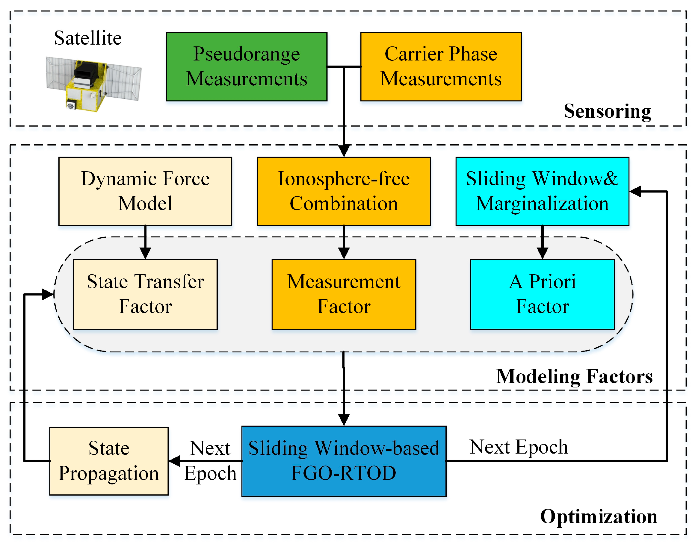
The implementation of the proposed sliding window-based FGO-RTOD framework is shown in Figure 3.

Step 1: At the initial epoch, the receiver position, velocity and clock offset are initialized using the SPP solution. LC ambiguities are initialized using Equation (29).

Step 2: Upon completion of the optimization in the previous epoch, states are propagated to the current epoch using Equations (26)–(29).

Step 3: Obtain raw measurements from the spaceborne receiver, including pseudoranges, carrier phases and broadcast ephemeris information, etc. Carrier phase cycle slip detection is implemented based on geometry-free (GF) combination [25].

Step 4: Construct the measurement factors, state transfer factors and a priori factor within the window. Then perform the optimization using Equation (30).

Step 5: Calculate the marginalization factor for the next epoch.

Step 6: Proceed to the subsequent epoch and iteratively execute Steps 2–5.

Due to the computation capacity limitation of the spaceborne processor, not all perturbations, especially minor ones such as solid Earth tides, ocean tides, polar tides, relativity effects, and Earth radiation pressure, should be considered in RTOD. The specific configurations for the dynamic force model are outlined in

Table 1. Relevant settings of dynamical model.

Items	Relevant Settings
Dynamical model
Earth gravity field	JGM3 (20 × 20) [26]
N-body gravitation	Moon and Sun only, low-precision analytic method [27]
Solid Earth tides	Neglected
Ocean tides	Neglected
Polar tides	Neglected
Solar radiation pressure	Cylindrical shadow model [28]
Atmosphere drag	Harris–Priester model (density) [29]
Earth radiation pressure and Relativity effects	Neglected
Reference frame
Coordinate system	J2000/WGS84
Precession and nutation	IAU1976/IAU 1980 simplified model
Earth rotation parameter	Rapidly predicted EOP in IERS Bulletin A

. In this paper, simplified precession and nutation models and rapidly predicted Earth orientation parameters are applied for the transformation of coordinate systems.

4. Experimental and Simulation Evaluations

We verified the performance of the proposed algorithm in two scenarios: the regular scenario and the challenging scenario. For the regular scenario, we used the onboard GNSS data of the GRACE-FO-A satellite which maintains a stable Earth-pointing attitude and carries a high-precision spaceborne GNSS receiver. Raw observation data could be obtained from the Level-1B products provided by the German Research Centre for Geosciences (GFZ). For the challenging scenario, we processed one set of data from the simulation platform and three sets of real data from Tianping-2B to validate the performance of the proposed method in this paper when the satellite is in a non-Earth-pointing attitude and a low-cost receiver is used. This is the first time that information about Tianping-2B has been made public. Tianping-2B is a microsatellite weighing about 20 kg and was launched in 2022. It flies in a sun-synchronous orbit at an altitude of about 500 km and employs adaptive attitude control aligned with mission-specific requirements.

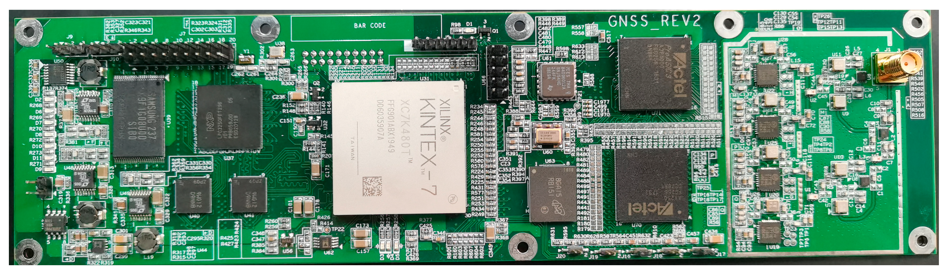
The ZJU-SpaceRcv GNSS receiver aboard the Tianping-2B satellite delivers position, velocity, and time (PVT) services while validating real-time orbit determination capabilities, as shown in Figure 4. It is a low-cost and miniaturized spaceborne receiver independently developed by Zhejiang University in Hangzhou, China and this is the first time that the receiver has been tested on orbit. ZJU-SpaceRcv can collect code and phase measurements at the L1C and L2C frequencies of the GPS or the B1I and B3I frequencies of both the BDS-2 and the BDS-3. To the best of the authors’ knowledge, this is the first on-orbit dual-civilian-code (L1C and L2C) spaceborne GPS receiver used for orbit determination. The relevant specifications of ZJU-SpaceRcv are listed in

Table 2. Specifications of the ZJU-SpaceRcv GNSS receiver.

Items	Relevant Settings
System	GPS or BDS
Receiving frequency	GPS: L1C/L2C BDS: B1I/B3I
Number of channels	12 each for each frequency
Measurement	Carrier phase, pseudorange, and Doppler
Sample interval	1 s
Carrier phase precision	≤6 mm
Pseudorange precision	≤2 m

.

Raw observations from the low-cost receiver on board Tianping-2B were used to validate the RTOD performance of the proposed method in the challenging scenario. We also used a GNSS simulator to simulate the GNSS signals received by Tianping-2B in space. The GNSS data processing strategies for GRACE-FO, Tianping-2B and the simulation are shown in

Table 3. GNSS data processing strategy.

Items	GRACE-FO	Tianping-2B/Simulation
GNSS signal	GPS L1P + L2P	GPS L1C + L2C
Combination	Undifferenced	Undifferenced
Sampling rate, s	30	10
Elevation cutoff, deg	5	-
Ionosphere	Dual-frequency ionosphere-free	Dual-frequency ionosphere-free
GNSS orbit and clock	Broadcast ephemeris	Broadcast ephemeris
Ambiguity	Float resolution	Float resolution

. The receiver antenna phase center offset (PCO) is corrected by satellite attitude information in quaternion. We ignore the effect of the antenna phase center variation (PCV) because it tends to be much smaller than the broadcast ephemeris error.

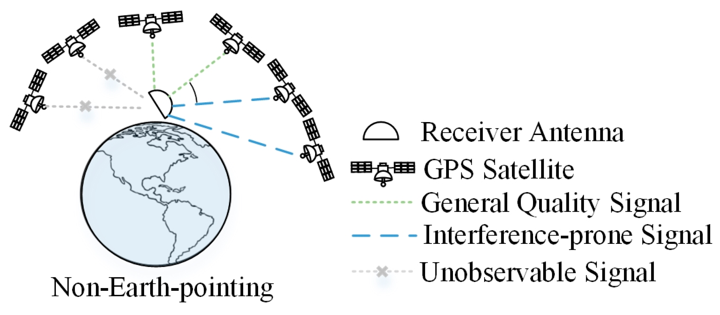
As shown in Figure 5, signals from satellites with high elevation angles typically yield more reliable observations. In contrast, signals from satellites with low or even negative elevation angles are susceptible to interference from atmospheric delays and severe multipath effects, which results in diminished measurement accuracy [30,31]. Consequently, it is essential to control the signal quality by setting an appropriate cut-off elevation angle for satellites in general missions. Since not all GPS satellites transmit L2C signals [32], there are fewer observations available for dual-frequency ionosphere-free (IF) combinations for ZJU-SpaceRcv. Furthermore, the number of visible satellites is significantly reduced when the microsatellite operates in a non-Earth-pointing attitude, necessitating the inclusion of low and negative elevation satellites to ensure positioning continuity. Compounding the issue, during microsatellite attitude maneuvers, the receiver’s internal loop may lose lock, leading to carrier phase cycle slips [33].

A priori standard deviation and process noise settings for GRACE-FO, Tianping-2B and the simulated microsatellite are shown in

Table 4. A priori standard deviation and process noise settings.

Items	GRACE-FO	Tianping-2B/Simulation
${\Pi }_{y0}$	$diag\left\{50.4, 50.4, 50.4, 1, 1, 1\right\}$
${\Pi }_{dtr0}$	400
$Q_D$	$\begin{array}{l}diag\left\{1, 1, 1, 1\times {10}^{-6}, 1\times {10}^{-6}, 1\times {10}^{-6}\right\}\hfill \end{array}$
$Q_C$	$4\times {10}^{-8}$	12.9
$Q_{N,12}^s$	$1\times {10}^{-8}$

.

4.1. Experimental Evaluation in Regular Scenario

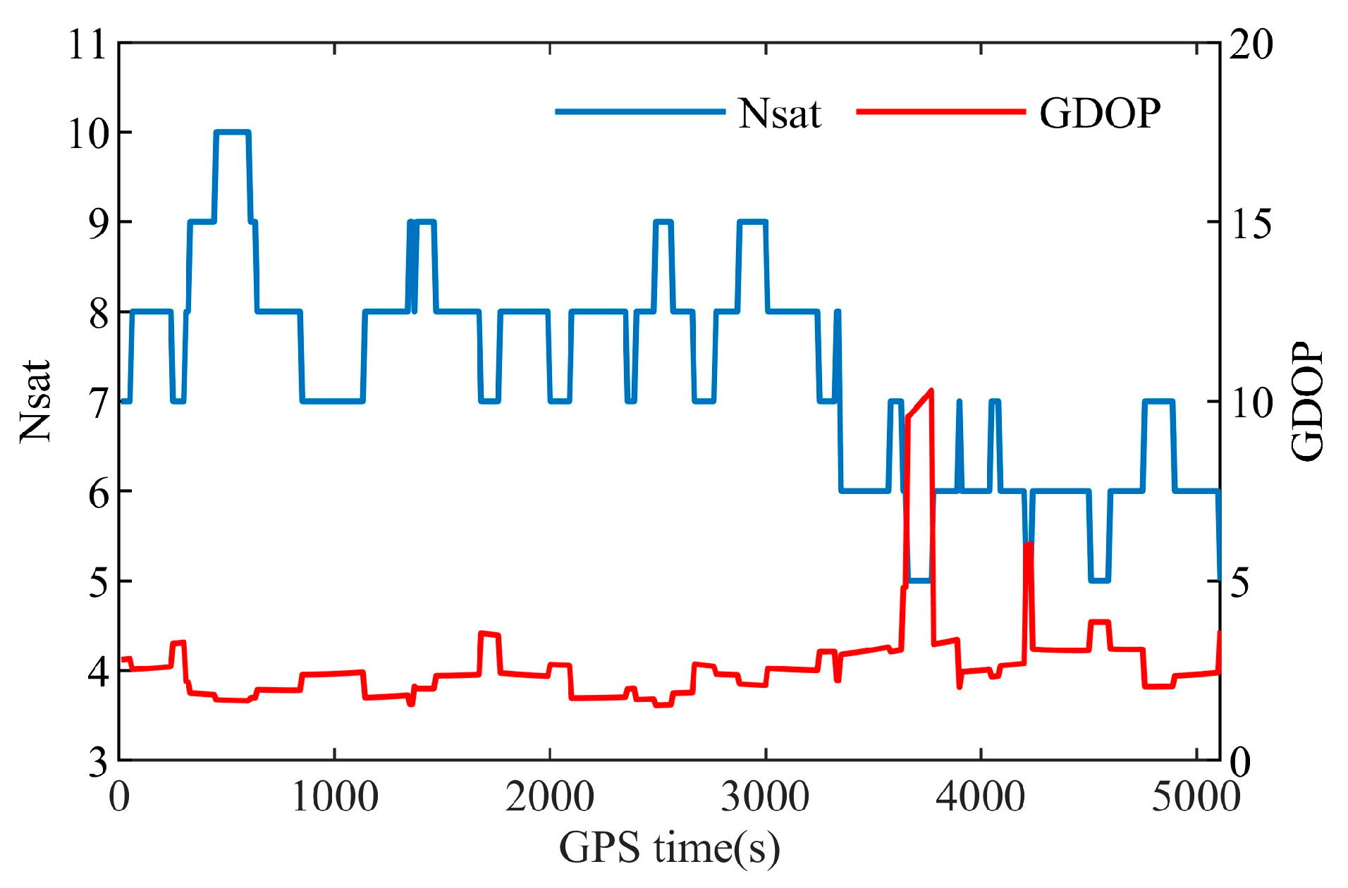
The GRACE-FO-A data from 0–24 h on 5 May 2019 was selected to evaluate the performance of the proposed algorithm in a regular scenario. The left part of Figure 6 presents a sky plot showing the distribution of observed satellites based on azimuth and elevation angle. It can be observed that the satellite distribution appears to be highly uniform, indicating that GRACE-FO-A is carrying out a stable observation of the Earth. GDOP quantitatively describes how satellite geometric configurations affect positioning accuracy. The number of satellites (Nsat) and GDOP for the entire arc segment are shown in the right part of Figure 6. The average number of observed satellites during the entire arc segment is 8.33. The GDOP remains within the range of 2 to 3, except for occasional instances when GDOP increases due to a decrease in the number of visible GPS satellites.

To comprehensively assess the efficacy of the proposed methodology, we conducted a comparative analysis of positioning performance across three different methods, noting that FGO did not introduce an M-estimator at this time:

(1)

EKF-RTOD: the standard EKF-based GNSS RTOD framework [4], where the measurement model and state transition model are derived from the factors in the FGO framework, and all relevant parameter settings are consistent with those used in the FGO framework;

(2)

FGO-RTOD: the proposed sliding window-based FGO-based RTOD framework with marginalization, which provides the real-time solution for the latest state node solved by Equation (30);

(3)

FGO-RTOD (Delayed): the method gives the delayed solution for the oldest state node in the sliding window with marginalization. The solution has a window-length time delay.

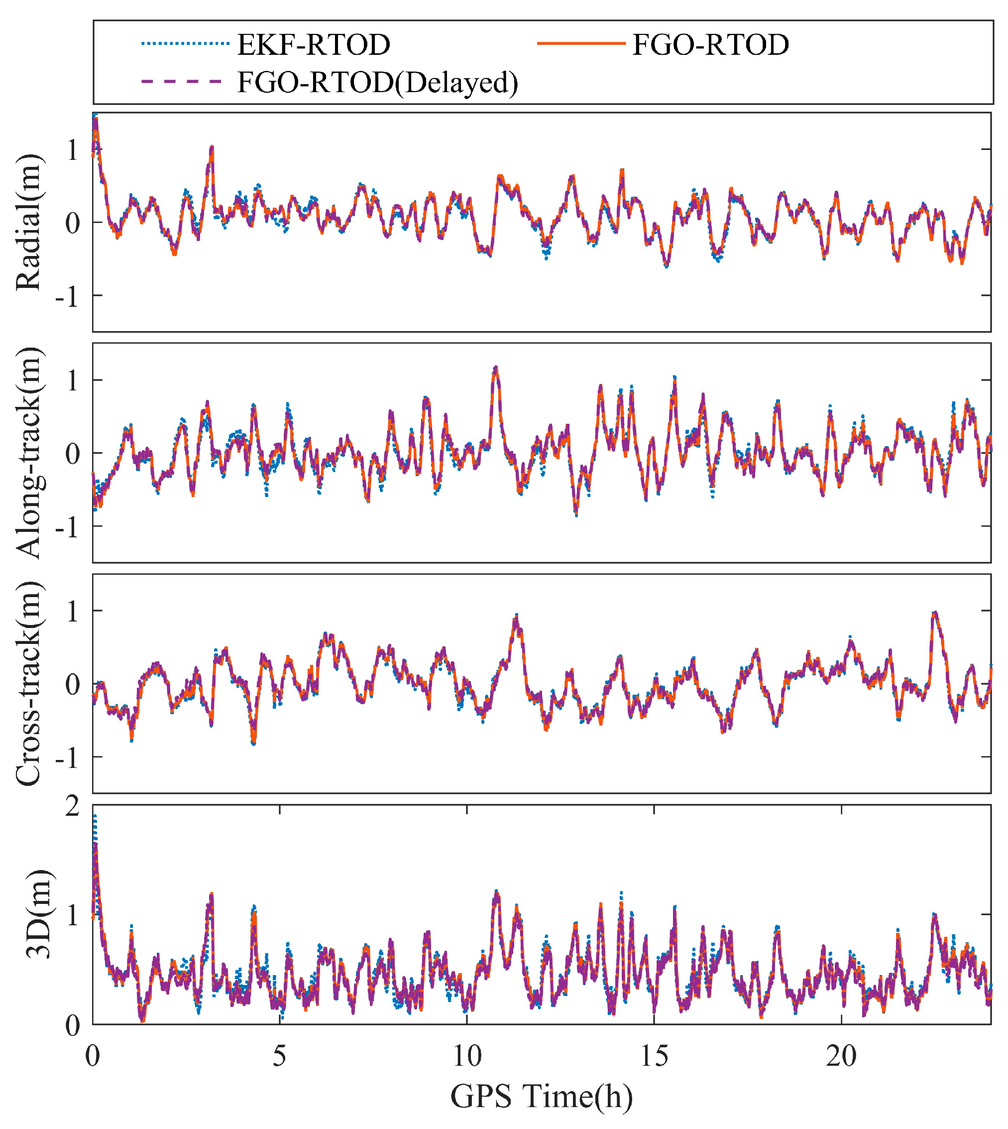
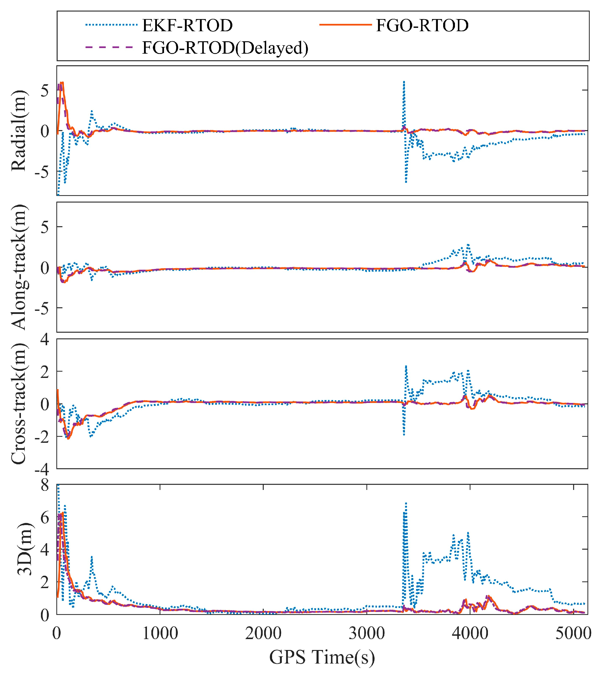
Positioning errors in radial direction, along-track direction, cross-track direction and 3D were derived from precision orbit references provided by the Jet Propulsion Laboratory (JPL), shown in Figure 7. Corresponding statistics are summarized in

Table 5. Statistics of positioning errors for GRACE-FO-A (unit m).

Modes	Radial	Along-Track	Cross-Track	3D
EKF-RTOD	0.257	0.315	0.300	0.505
FGO-RTOD	0.255	0.306	0.302	0.499
FGO-RTOD(Delayed)	0.243	0.303	0.296	0.488

. Comparative analysis reveals that FGO-RTOD achieves marginally superior accuracy relative to EKF-RTOD in the regular scenario, which is indeed attributed to the advantages of the FGO method, such as multiple iterations, re-linearization, and the ability to take into account the correlation of multiple epochs. However, since the quality of the observed data is high in the current scenario, the problem tends to be highly linear and the benefits of re-linearization may be limited. In addition, the state variations between epochs in the regular scenario are very stable, so the advantages of FGO, which can take into account multiple epoch correlations, over the sequential estimator EKF cannot be exploited, resulting in limited accuracy improvement. FGO-RTOD(Delayed) exhibits improved accuracy compared to FGO-RTOD due to the consideration of additional nodes and factors, however, we do not describe it too much because it cannot obtain a real-time solution.

4.2. Simulation Evaluation in Challenging Scenario

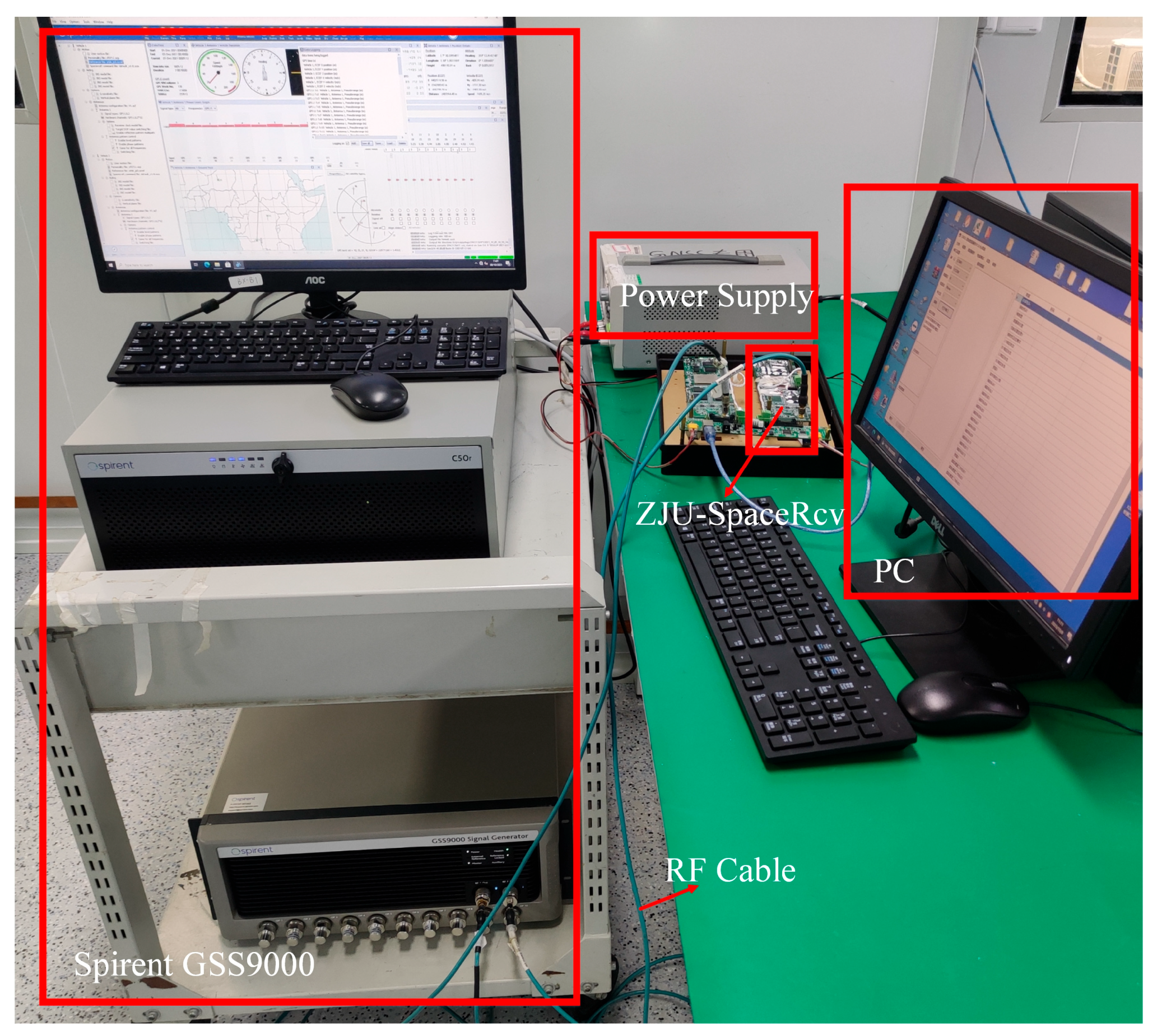
The simulation hardware setup is shown in Figure 8, which includes a GNSS signal simulator, a ZJU-SpaceRcv GNSS receiver, a PC, an RF cable and a power supply. The GNSS signal simulator used in this setup is the Spirent GSS9000, which is capable of simulating GPS L1C and L2C signals. ZJU-SpaceRcv received the RF signals from the simulator and forwarded the raw GNSS observations to the PC.

The specific orbital parameters are provided in

Table 6. Orbital elements of the simulated microsatellite.

Orbital Elements	a, m	e	i, deg	Ω, deg	ω, deg	M, deg
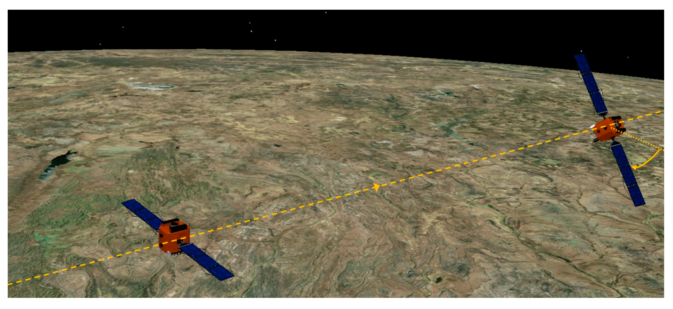
Settings	6,893,818.8336	0.0005910	97.4391	−64.3989	−108.7805	179.4492

. At the beginning, the simulated microsatellite was in the Earth-pointing attitude until 3500 s, when it began to roll at a speed of +1 deg/s, as shown in Figure 9. Once the roll angle reached 45 deg, the attitude was fixed for 5 min. Afterward, the microsatellite returned to the normal Earth-pointing attitude at a rate of −1 deg/s.

The Nsats and GDOPs in the simulation are displayed in Figure 10. During the simulation, the number of satellites available for RTOD fluctuates between 5 and 10, with an average of 7.3. The GDOP varies between 1.53 and 10.31. During the period of satellite rolling, the number of available satellites for RTOD significantly decrease to the minimum, with a corresponding increase in GDOP to the maximum.

The positioning errors are illustrated in Figure 11, with the true orbits are given from the GNSS simulator. Corresponding statistics are summarized in

Table 7. Statistics of positioning errors for the simulated microsatellite (unit m).

Modes	Radial	Along-Track	Cross-Track	3DRMS	3DMAX
EKF-RTOD	1.267	0.689	0.573	1.552	6.921
FGO-RTOD	0.139	0.258	0.142	0.326	1.139
FGO-RTOD (Delayed)	0.139	0.256	0.136	0.321	1.130

. The results demonstrate that the stability of FGO-RTOD is markedly superior to that of EKF-RTOD during the satellite’s attitude maneuver, with the 3D maximum (3DMAX) errors for FGO-RTOD and EKF-RTOD being 1.139 m and 6.921 m, respectively. Meanwhile, the positioning error of FGO-RTOD exhibits significantly smoother behavior, and its 3DRMS is reduced by 79.0% compared to that of EKF-RTOD. Furthermore, upon restoration of the number of available satellites, FGO-RTOD achieves faster convergence and higher accuracy than EKF-RTOD. The reason why FGO-RTOD achieves better results compared to EKF-RTOD lies in the fact that EKF-RTOD can be viewed as an FGO-RTOD with a sliding window length of 1, while FGO-RTOD can simultaneously consider the correlations among all epochs within a sliding window of length n. Measurement outliers in individual epochs are constrained by the epoch-to-epoch correlations in FGO, making it difficult for them to affect the normal states within the window. This enables FGO-RTOD to identify measurement outliers more effectively.

4.3. Experimental Evaluation in Challenging Scenario

Raw GNSS observations collected from Tianping-2B in July 2023 were used to evaluate the performance of the proposed algorithm in the challenging scenario. Given the constrained battery capacity of the microsatellite, the ZJU-SpaceRcv GNSS receiver was only powered on during complex tasks requiring accurate positioning information. The specific arc segments analyzed in this paper were:

Arc1: started on 07/18/2023 23:03:00, ended on 07/19/2023 02:03:00.

Arc2: started on 07/20/2023 10:32:50, ended on 07/20/2023 11:48:00.

Arc3: started on 07/21/2023 23:05:00, ended on 07/22/2023 02:00:00.

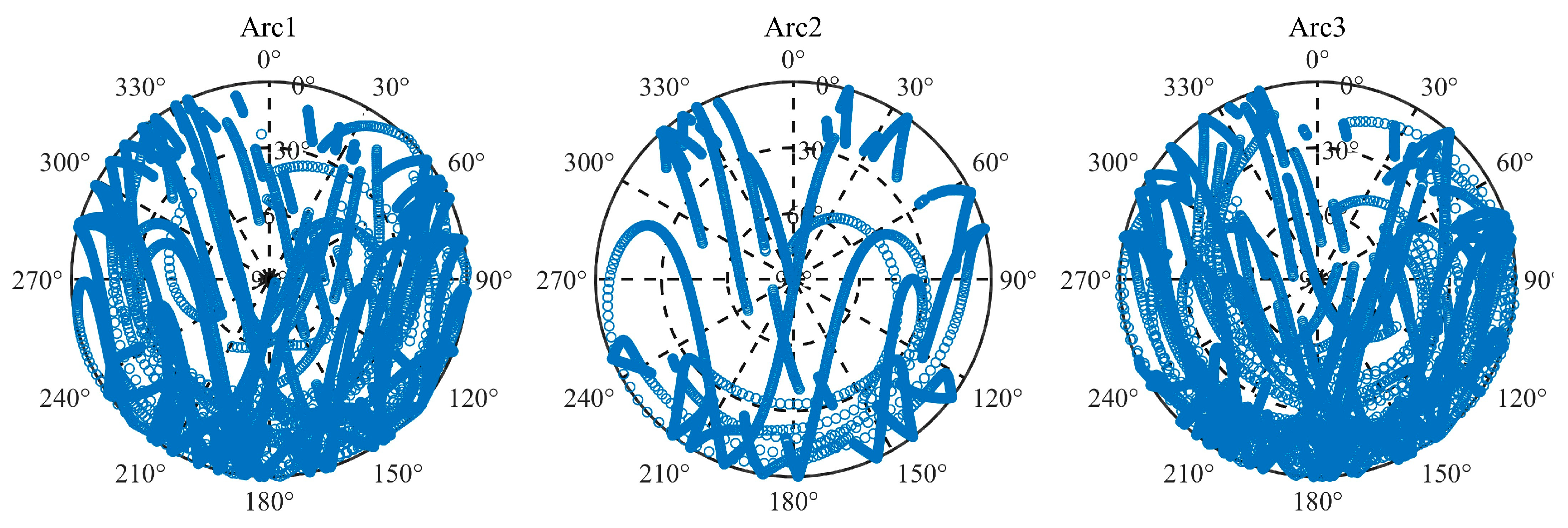
The sky plot of the observed GPS satellites is depicted in Figure 12. It is evident from the plot that there is a gap in the azimuth range of 350° to 30°. This gap suggests that Tianping-2B was not pointing to the center of the Earth during the corresponding flight arc.

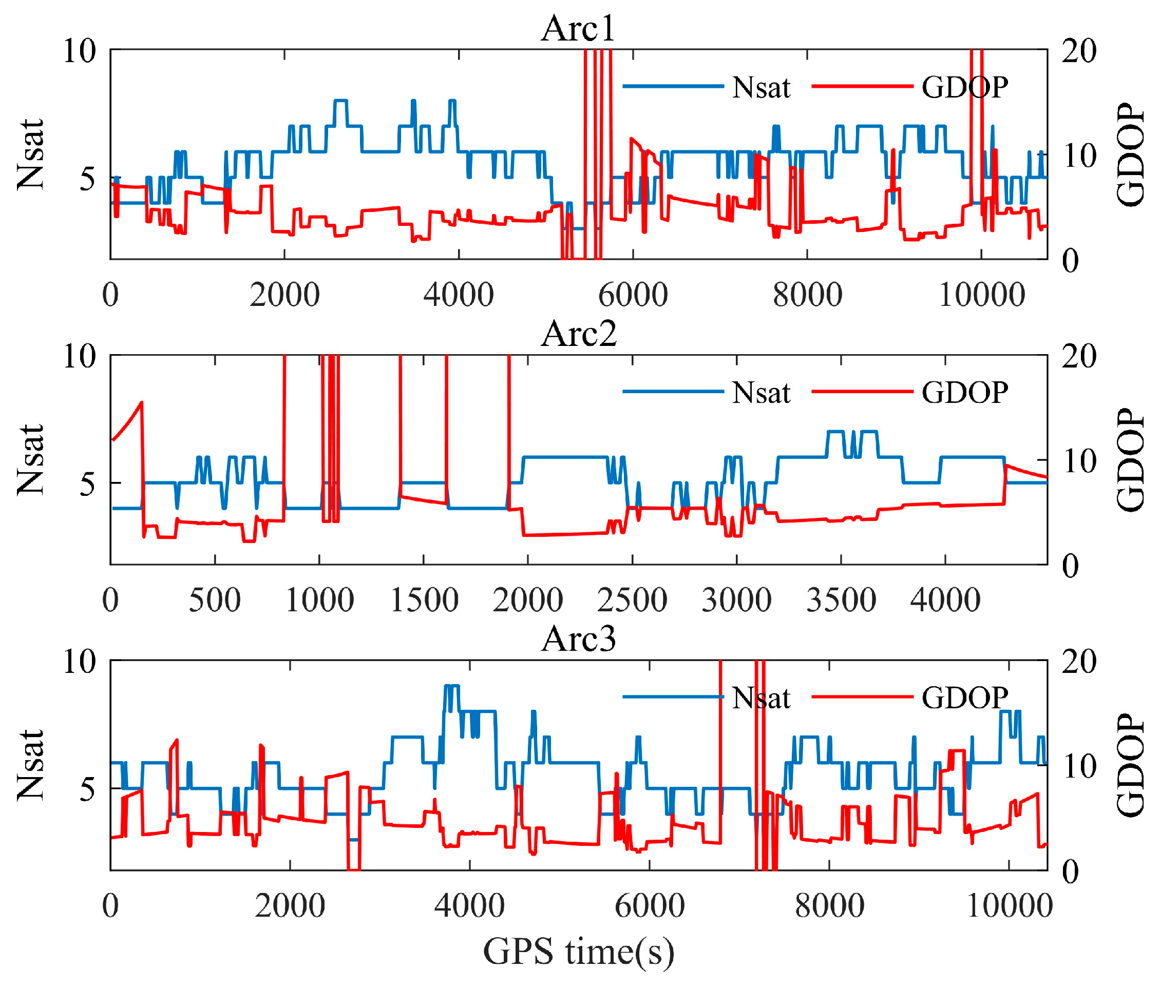
The Nsats and GDOPs for the three arc segments are displayed in Figure 13. As ZJU-SpaceRcv operates at the L2C frequency, the number of observations available for dual-frequency IF combination is considerably lower compared to GRACE-FO. Consequently, there are moments when the GDOP drops to 0 due to the Nsat falling below 4. The data from Tianping-2B can be used to evaluate the robustness of the proposed algorithm in the challenging scenario.

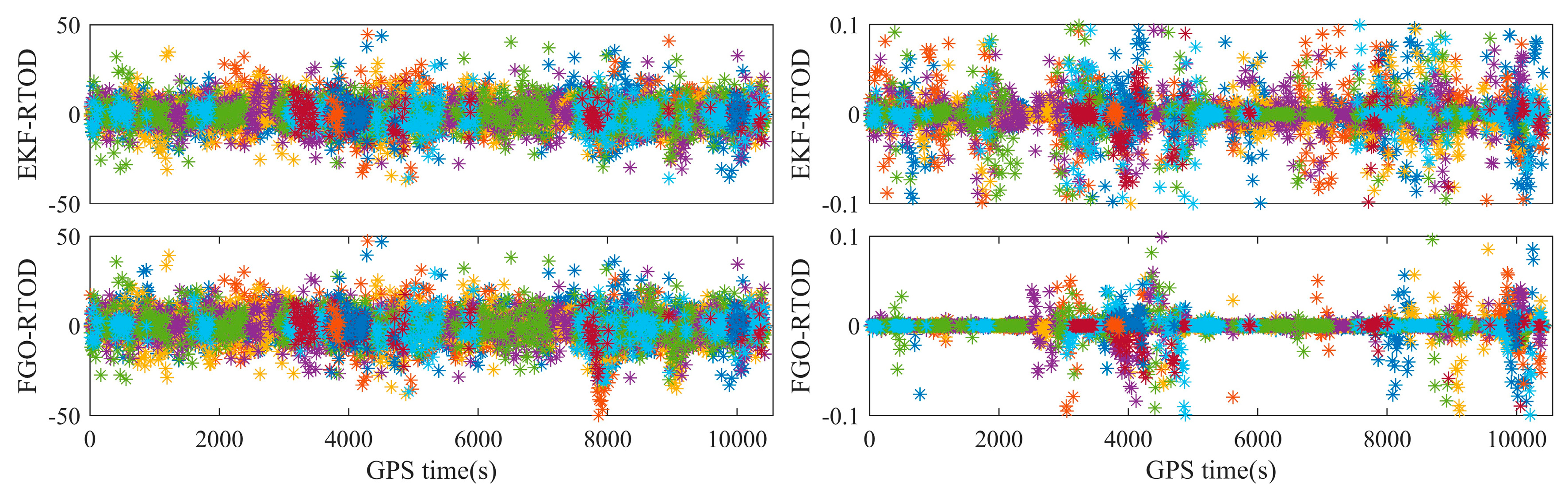
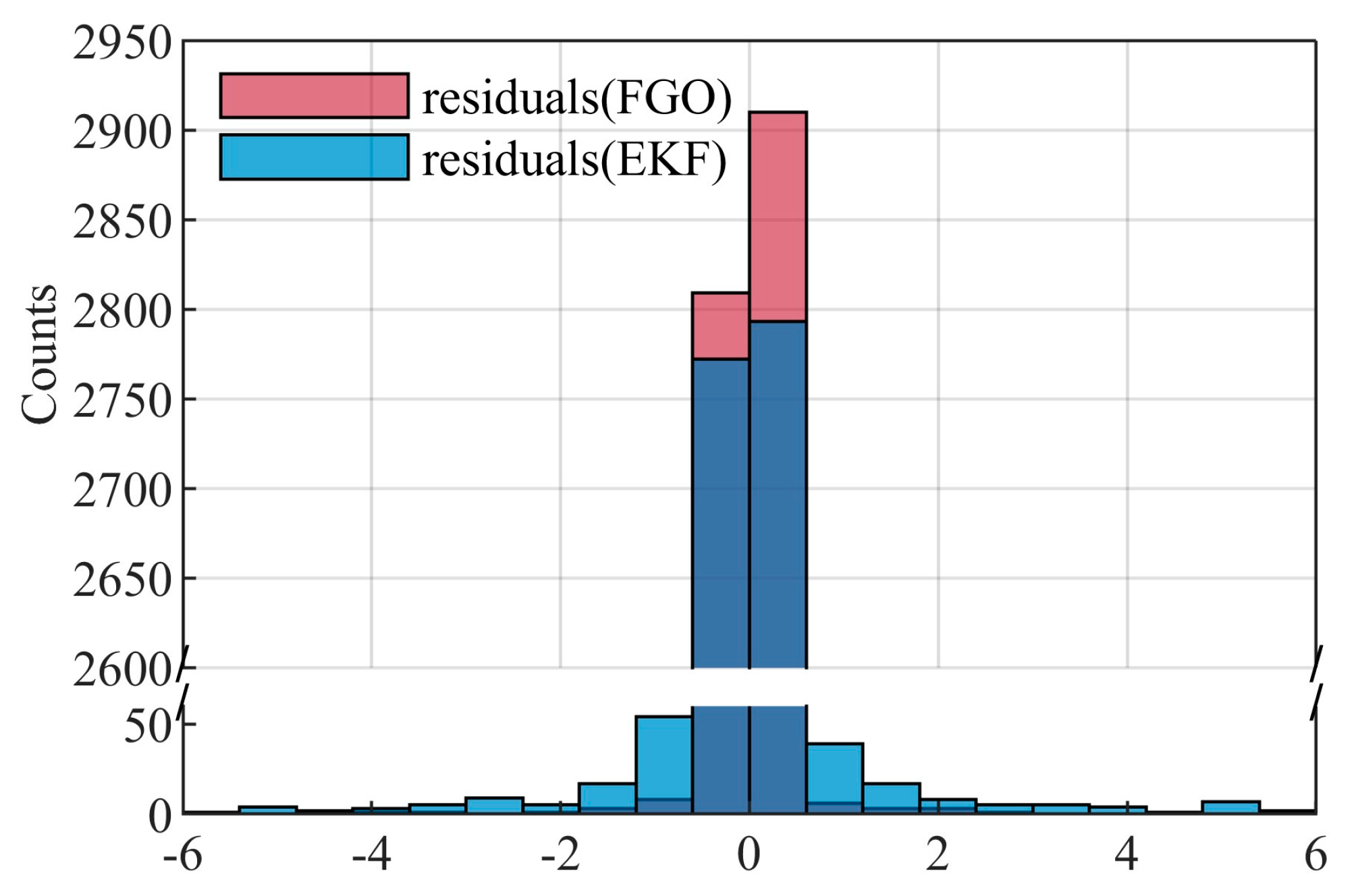
Tianping-2B is equipped exclusively with ZJU-SpaceRcv for positioning, and no reference orbit is available for performance assessment. Furthermore, the short observational arcs preclude the comparison of overlapping arcs. Therefore, we illustrated the algorithm’s performance through the residuals of PC and LC. The residuals of PC and LC for Arc3 are shown in Figure 14. It is evident that the LC residuals of FGO-RTOD exhibit a considerable reduction in the number of discrete points compared to those of EKF-RTOD. Histograms of LC residuals of EKF-RTOD and FGO-RTOD are shown in Figure 15. Note that the dark blue bin indicates an overlap between FGO’s LC residual count and EKF’s. As illustrated in Figure 15, FGO demonstrates a superior ability to concentrate the LC residuals around zero and to identify unreliable outliers more effectively than EKF.

The residuals of non-outlier LC measurements typically remain below 10 cm.

Table 8. RMS and ratio of LC residuals less than 10 cm for Tianping-2B.

Modes	Arc1		Arc2		Arc3
	RMS (cm)	Ratio (%)	RMS (cm)	Ratio (%)	RMS (cm)	Ratio (%)
EKF-RTOD	2.050	88.50	2.199	91.19	2.052	90.57
FGO-RTOD	1.619	95.49	1.351	99.08	1.051	97.90

shows the Root Mean Square (RMS) of LC residuals for EKF-RTOD and FGO-RTOD across the three arcs, considering only LC residuals below 10 cm. In addition, Table 8 includes the ratio between the number of LC residuals less than 10 cm and the total number of LC residuals. The LC residuals RMS for FGO-RTOD of Arc3 significantly decreases from 2.052 cm to 1.051 cm, while the ratio of LC residuals below 10 cm increases from 90.57% to 97.90%. For other arcs, the improvements in RMS and ratio exceed 0.43 cm and 7.0%, respectively. These results further underscore the superior capability of FGO-RTOD in managing LC outliers compared to EKF-RTOD in the challenging scenario.

5. Discussion

Using an M-estimator is a typical way to reduce the sensitivity to outliers. The objective function of FGO-RTOD with the Cauchy function is expressed as:

$$\widehat{\chi }=\underset{\chi }{\arg \min }\left\{{‖e_x\left(k-n+1\right)‖}_{\Pi \left(k-n+1\right)}^2+{\displaystyle \sum _n\mathit{\gamma }\left({‖e_z\left(k\right)‖}_{R(k)}^2\right)+{\displaystyle \sum _{n-1}\left({‖e_f\left(k\right)‖}_{Q(k)}^2\right)}}\right\}$$

(31)

The Cauchy function is applied as follows [11]:

$$\gamma \left(e\right)={\displaystyle \frac{{\varrho }^2}{2}}\log \left(1+{\displaystyle \frac{e^2}{{\varrho }^2}}\right)$$

(32)

where $\varrho$ denotes the kernel parameter.

This section discusses the effect of different sliding window lengths and different M-estimator settings on the performance of FGO-RTOD. All tests were conducted using a high-performance laptop computer with an AMD CPU (Ryzen 7 5800 H) at 3.20 GHz and 16 GB RAM. The first hour RTOD solutions for GRACE-FO-A are presented in Figure 16. FGO-RTOD(Batch) is the solution of the batch estimator with incrementally expanding window length, and FGO-RTOD(3) and FGO-RTOD(5) are the solutions with marginalization for sliding window lengths of 3 and 5, respectively. Figure 16 show that FGO-RTOD(Batch) demonstrates superior positioning accuracy at the beginning due to the consideration of information from more epochs. However, its accuracy exhibits negligible improvement over time relative to the sliding window implementations with marginalization—a trend aligning precisely with theoretical predictions [16,22]. As the number of states requiring optimization in FGO-RTOD(Batch) increases over time, its computational runtime also grows significantly, exceeding that of FGO-RTOD. Consequently, FGO-RTOD(Batch) is unsuitable for real-time processing applications. In contrast, FGO-RTOD maintains a consistent runtime once the sliding window is fully populated, achieving a runtime of less than 1 s with an appropriately configured window length, thereby fulfilling real-time processing requirements.

Table 9. FGO-RTOD statistics for the simulated microsatellite with different sliding window lengths.

Window Length	2	3	4	5
Mean runtime (s)	0.039	0.100	0.206	0.327
RMS (m)	0.329	0.326	0.320	0.316

presents the influence of varying window lengths on FGO-RTOD performance in the challenging scenario simulation. Analysis reveals a progressive reduction in positioning error RMS with increasing window length. This enhanced precision occurs at the cost of exponentially increasing computational time. Different robust function settings can also affect the results differently. As shown in

Table 10. FGO-RTOD statistics for the simulated microsatellite with different settings of the M-estimator.

Robust Function	NULL	Cauchy (1)	Cauchy (10)	Cauchy (20)
RMS (m)	0.326	0.334	0.324	0.325

, when the kernel parameter is set to 1, the algorithm exhibits suboptimal positioning accuracy, which is even lower than the accuracy achieved without using a robust function. This is likely due to the inappropriate downweighting of high-precision measurements, leading to a degradation in overall performance. In contrast, when the kernel parameter of the Cauchy function is set to 10 and 20, the algorithm’s accuracy improves, with the highest accuracy achieved at a kernel parameter of 10. This demonstrates that, in the current simulation, using an appropriate robust function can further mitigate the impact of low-quality measurements.

The influence of varying window lengths and M-estimator configurations on the performance of FGO in the challenging scenario experiment of Arc3 is detailed in

Table 11. FGO-RTOD statistics for Tianping-2B with different sliding window lengths.

Window Length	2	3	4	5
Mean runtime (s)	0.070	0.218	0.466	0.833
LC residual RMS (cm)	1.087	1.051	1.052	1.042
Ratio (%)	97.98	97.90	97.90	97.83

and

Table 12. FGO-RTOD statistics for Tianping-2B with different settings of the M-estimator.

P	NULL	Cauchy (1)	Cauchy (10)	Cauchy (20)
LC residual RMS (cm)	1.051	1.289	1.048	1.064
Ratio (%)	97.90	82.34	97.59	97.72

. As the window length increases, the LC residual RMS generally shows a decreasing trend, which to some extent reflects the improving effectiveness of the algorithm. The ratio decreases as the window length increases because the algorithm incorporates more LC ambiguity variation factors, prioritizing the consistency of LC ambiguities across epochs over the minimization of residual magnitudes. The results presented in Table 12 demonstrate that the LC residual RMS is minimized when employing the Cauchy function with a kernel parameter of 10. As the kernel parameter increases, the ratio also increases, indicating that more LCs are trusted, with the maximum ratio occurring in the algorithm without a robust function, which is consistent with the theory.

6. Conclusions and Outlooks

This paper proposes an FGO-based RTOD method aiming at achieving robust and accurate positioning for microsatellites operating in challenging scenarios. The proposed method incorporates dynamics factors, clock offset variation factors, and LC ambiguity variation factors to model temporal correlations between state nodes. In the sliding window-based FGO estimator, a Schur complement-based marginalization method is employed to preserve out-of-window state node information.

In the experimental part, the accuracy of FGO-RTOD was verified by using data from GRACE-FO-A. Comparative analyses demonstrate marginally superior precision for FGO-RTOD over EKF-RTOD in the regular scenario. The simulation results show that the accuracy of FGO-RTOD is significantly better than that of EKF-RTOD during the time period when the satellite is performing attitude maneuvers, and the positioning error of FGO-RTOD is significantly smoother throughout the simulation. The results obtained from Tianping-2B demonstrate that FGO-RTOD exhibits markedly smaller LC residuals and a significantly higher ratio of LC residuals below 10 cm compared to EKF-RTOD. These findings indicate that FGO-RTOD effectively manages outlier measurements in challenging scenarios and outperforms EKF-RTOD. Experiments conducted with varying window lengths reveal that, in most cases, increasing the window length improves the algorithm’s performance, albeit at the cost of greater computational time. Furthermore, the choice of loss functions can exert distinct influences on the algorithm’s performance.

FGO-RTOD in this paper was developed based on Eigen, Ceres solver and some basic libraries, and it is feasible for them to be deployed on a satellite computer. The inputs to FGO-RTOD including broadcast ephemeris, pseudorange, and carrier phase observations are available in real-time through the spaceborne GNSS receiver, so the algorithm has few limitations when working on a microsatellite. In future works, we will deploy the FGO on a satellite computer, conduct a detailed time/space complexity analysis of the algorithm, and obtain the performance of FGO-RTOD via a satellite-ground data transmission link.

References

- Lin, C.; Jin, X.; Mo, S.; Hou, C.; Zhang, W.; Xu, Z.; Jin, Z. Performance analysis and validation of precision multisatellite RF measurement scheme for microsatellite formations. Meas. Sci. Technol. 2022, 33, 025001. [Google Scholar] [CrossRef]
- Xu, J.; Zhang, C.; Wang, C.; Jin, Z. Novel Approach to Intersatellite Time-Difference Measurements for Microsatellites. J. Guid. Control Dyn. 2018, 41, 2476–2482. [Google Scholar] [CrossRef]
- Hou, C.; Jin, X.; Zhou, L.; Wang, H.; Yang, X.; Xu, Z.; Jin, Z. Precision Joint RF Measurement of Inter-Satellite Range and Time Difference and Scalable Clock Synchronization for Multi-Microsatellite Formations. Sensors 2023, 23, 4109. [Google Scholar] [CrossRef] [PubMed]
- Montenbruck, O.; Ramos-Bosch, P. Precision real-time navigation of LEO satellites using global positioning system measurements. Gps Solut. 2008, 12, 187–198. [Google Scholar] [CrossRef]
- Wang, F.; Gong, X.; Sang, J.; Zhang, X. A Novel Method for Precise Onboard Real-Time Orbit Determination with a Standalone GPS Receiver. Sensors 2015, 15, 30403–30418. [Google Scholar] [CrossRef] [PubMed]
- Kschischang, F.R.; Frey, B.J.; Loeliger, H.A. Factor graphs and the sum-product algorithm. IEEE Trans. Inf. Theory 2001, 47, 498–519. [Google Scholar] [CrossRef]
- Li, X.; Wang, X.; Liao, J.; Li, X.; Li, S.; Lyu, H. Semi-tightly coupled integration of multi-GNSS PPP and S-VINS for precise positioning in GNSS-challenged environments. Satell. Navig. 2021, 2, 1. [Google Scholar] [CrossRef]
- Dellaert, F.; Kaess, M. Factor graphs for robot perception. Found. Trends Robot. 2017, 6, 1–139. [Google Scholar]
- Wang, X.; Li, X.; Shen, Z.; Li, X.; Zhou, Y.; Chang, H. Factor graph optimization-based multi-GNSS real-time kinematic system for robust and precise positioning in urban canyons. Gps Solut. 2023, 27, 200. [Google Scholar] [CrossRef]
- Taylor, C.; Gross, J. Factor Graphs for Navigation Applications: A Tutorial. Navig.-J. Inst. Navig. 2024, 71, navi.653. [Google Scholar] [CrossRef]
- Bai, X.; Wen, W.; Hsu, L.-T. Time-Correlated Window-Carrier-Phase-Aided GNSS Positioning Using Factor Graph Optimization for Urban Positioning. IEEE Trans. Aerosp. Electron. Syst. 2022, 58, 3370–3384. [Google Scholar] [CrossRef]
- Wen, W.; Zhang, G.; Hsu, L.-T. GNSS Outlier Mitigation via Graduated Non-Convexity Factor Graph Optimization. IEEE Trans. Veh. Technol. 2022, 71, 297–310. [Google Scholar] [CrossRef]
- Sünderhauf, N.; Protzel, P. Towards robust graphical models for GNSS-based localization in urban environments. In Proceedings of the International Multi-Conference on Systems, Signals & Devices, Chemnitz, Germany, 20–23 March 2012. [Google Scholar]
- Watson, R.M.; Gross, J.N. Evaluation of Kinematic Precise Point Positioning Convergence with an Incremental Graph Optimizer. In Proceedings of the IEEE/ION Position, Location and Navigation Symposium (PLANS), Monterey, CA, USA, 23–26 April 2018. [Google Scholar]
- Wen, W.; Hsu, L.-T. Towards robust GNSS positioning and real-time kinematic using factor graph optimization. In Proceedings of the 2021 IEEE International Conference on Robotics and Automation (ICRA), Yokohama, Japan, 30 May 2021. [Google Scholar]
- Xin, S.; Geng, J.; Hsu, L.-T. Factor Graph Optimization-Based GNSS PPP-RTK: An Alternative Platform to Study Urban GNSS Precise Positioning. IEEE Trans. Aerosp. Electron. Syst. 2024, 60, 3221–3236. [Google Scholar] [CrossRef]
- An, X.; Meng, X.; Jiang, W. Multi-constellation GNSS precise point positioning with multi-frequency raw observations and dual-frequency observations of ionospheric-free linear combination. Satell. Navig. 2020, 1, 7. [Google Scholar] [CrossRef]
- Zhao, X.; Zhou, S.; Ci, Y.; Hu, X.; Cao, J.; Chang, Z.; Tang, C.; Guo, D.; Guo, K.; Liao, M. High-precision orbit determination for a LEO nanosatellite using BDS-3. Gps Solut. 2020, 24, 102. [Google Scholar] [CrossRef]
- Tancredi, U.; Renga, A.; Grassi, M. Real-Time Relative Positioning of Spacecraft over Long Baselines. J. Guid. Control Dyn. 2014, 37, 47–58. [Google Scholar] [CrossRef]
- Kroes, R.; Montenbruck, O.; Bertiger, W.; Visser, P. Precise GRACE baseline determination using GPS. Gps Solut. 2005, 9, 21–31. [Google Scholar] [CrossRef]
- Iwase, T.; Kojima, Y.; Teramoto, E. M-Epoch Ambiguity Resolution Technique for Single Frequency Receivers with INS Aid. In Proceedings of the IEEE/ION Position Location and Navigation Symposium (PLANS), Myrtle Beach, SC, USA, 23–26 April 2012. [Google Scholar]
- Sibley, G.; Matthies, L.; Sukhatme, G. Sliding Window Filter with Application to Planetary Landing. J. Field Robot. 2010, 27, 587–608. [Google Scholar] [CrossRef]
- Kaess, M.; Ranganathan, A.; Dellaert, F. iSAM: Incremental Smoothing and Mapping. IEEE Trans. Robot. 2008, 24, 1365–1378. [Google Scholar] [CrossRef]
- Agarwal, S.; Mierle, K. Ceres solver: Tutorial & reference. Google Inc 2012, 2, 8. [Google Scholar]
- Hatch, R. The synergism of GPS code and carrier measurements. In Proceedings of the International Geodetic Symposium on Satellite Doppler Positioning, Las Cruces, NM, USA, 8–12 February 1982. [Google Scholar]
- Tapley, B.D.; Watkins, M.; Ries, J.; Davis, G.; Eanes, R.; Poole, S.; Rim, H.; Schutz, B.; Shum, C.; Nerem, R.S. The joint gravity model 3. J. Geophys. Res. Solid Earth 1996, 101, 28029–28049. [Google Scholar] [CrossRef]
- Montenbruck, O.; Pfleger, T. Astronomy on the Personal Computer; Springer: Heidelberg, Germany, 2013. [Google Scholar]
- Montenbruck, O.; Gill, E.; Lutze, F. Satellite Orbits: Models, Methods, and Applications; Springer: Heidelberg, Germany, 2002. [Google Scholar]
- Cappellari, J.O.; Vélez, C.; Fuchs, A.J. Mathematical Theory of the Goddard Trajectory Determination System; Goddard Space Flight Center: Maryland, MD, USA, 1976. [Google Scholar]
- Montenbruck, O.; Kroes, R. In-flight performance analysis of the CHAMP BlackJack GPS Receiver. GPS Solut. 2003, 7, 74–86. [Google Scholar] [CrossRef]
- Wanninger, L.; May, M. Carrier-Phase Multipath Calibration of GPS Reference Stations. Navigation 2001, 48, 112–124. [Google Scholar] [CrossRef]
- Marques, H.A.S.; Monico, J.F.G.; Marques, H.A. Performance of the L2C civil GPS signal under various ionospheric scintillation effects. Gps Solut. 2016, 20, 139–149. [Google Scholar] [CrossRef]
- Kim, J.W.; Shin, M.Y.; Melin, L.; Hwang, D.-H.; Lee, S.J. GNSS receiver rotation tracking loop design for spinning vehicles. In Proceedings of the IEEE/ON Position, Location and Navigation Symposium, Monterey, CA, USA, 5–8 May 2008. [Google Scholar]
Figure 1.
Sliding window-based factor graph of RTOD.
Figure 2.
Acceleration vectors of the LEO satellite.
Figure 3.
Implementation of sliding window-based FGO-RTOD framework.
Figure 4.
ZJU-SpaceRcv GNSS receiver.
Figure 5.
Quality of signals received when the microsatellite is in non-Earth-pointing attitude.
Figure 6.
Distribution of observed satellites (left), and Nsat and GDOP (right) for GRACE-FO-A.
Figure 7.
Positioning errors for GRACE-FO-A.
Figure 8.
Hardware setup.
Figure 9.
Microsatellite is rolling to fulfill the earth observation mission.
Figure 10.
Nsat and GDOP for the simulated microsatellite.
Figure 11.
Positioning errors for the simulated microsatellite.
Figure 12.
Distribution of observed satellites for Tianping-2B.
Figure 13.
Nsat and GDOP for Tianping-2B.
Figure 14.
PC (left) and LC (right) residuals for Tianping-2B.
Figure 15.
Histogram of LC residuals for Tianping-2B.
Figure 16.
Positioning error and runtime of RTOD for GRACE-FO-A.