High-Precision Centroid Localization Algorithm for Star Sensor Under Strong Straylight Condition

Abstract

Star sensor is disturbed by strong straylight, which increases the gray level of the captured star map, and this leads to invalid detection of star points and affects the high-precision location of the centroid. To address this issue, we propose a star centroid localization method based on gradient-oriented multi-directional local contrast enhancement. First, the background gray level distribution patterns of star sensors under various actual straylight interference conditions are analyzed. Based on this analysis, a background imaging model for complex operational scenarios is established. Finally, simulations are conducted under complex conditions with straylight images to test the star point detection rate, false detection rate, centroid localization accuracy, and statistical significance testing. The results show that the proposed algorithm outperforms the TOP-HAT, MAX-BACKG (Max-Background Filtering), LCM (Local Contrast Measure), MPCM (Multiscale Patch-Based Contrast Measure), and CMLCM (Curvature-Based Multidirectional Local Contrast Method for Star Detection of Star Sensor) algorithms in terms of star point detection rate. Additionally, the RMSE centroid localization error is achieved with 0.1 pixels, demonstrating its ability to effectively locate star centroids under complex conditions and meet certain engineering application requirements.

1. Introduction

A star tracker is an astronomy sensor that uses stars as its target. It has several advantages, including high autonomy, exact measurements, no cumulative errors, small size, and mass [1,2,3,4,5]. As a result, star trackers are widely used in a variety of applications, including near-Earth satellites, deep space research, and ballistic missiles [6,7,8,9]. The star tracker gathers radiation from the target stars and straylight from sources such as sunlight, moonlight, Earth-atmosphere light, and Earth’s thermal emissions [10]. A strong straylight will form a non-uniform background gray scale on the image plane of the star sensor, reducing the contrast of the image plane and the signal-to-noise ratio of the star, making it difficult to extract the background noise [11], affecting the centroid extraction accuracy and the accuracy of astronomical navigation. As a result, current star sensor development trends are mostly focused on downsizing [12] and low power consumption. Please note that as the star sensor gets smaller, so does the lens hood, resulting in a dramatic reduction in the shading effect [13]. As a result, it is very crucial to offer a novel approach to star recognition and high-precision centroid localization [14,15].

Currently, there are three types of methods for removing the influence of intense straylight from star images: algorithms based on spatial domain filtering, algorithms based on frequency domain filtering, and algorithms inspired by the human visual system. Early weak target detection methods mostly used spatial domain filtering algorithms. Marvasti [16] devised a new morphological operation and built a novel Top-Hat transformation, which tackles the issue of existing Top-Hat transformations being unable to discriminate genuine targets in infrared weak target detection. Researchers had improved frequency domain filtering approaches by applying methods such as wavelet transform and shear wave transform [17]. Furthermore, several methods used singular value decomposition [18] to change the corresponding coefficients for target detection. However, these solutions were frequently confined by parameter setup constraints and may not be applicable to all cases. Overall, frequency domain filtering algorithms tend to be more sophisticated than spatial domain filtering techniques. Given that there was a significant gradient difference in grayscale values between the neighborhood image and the weak targets in the image, which corresponded to characteristics observed by the human visual system, local features were better suited to represent small targets and facilitate detection. Chen et al. [19] solved the issue of limited global feature representation by applying the local contrast measure (LCM) to accomplish poor target detection. The fundamental premise is to enhance and detect targets by using the local contrasts between small targets and background regions. However, this method is unsuitable for dim targets and has high computation times due to the usage of “sliding window” techniques for local contrast calculation, which might result in “block effect” distortions. Wei et al. [20], drawing on biological visual systems, used a multiscale patch-based technique to produce local contrast enhancement for target detection. This approach modulates the contrast between targets and backgrounds, allowing for the detection of both bright and dim targets via threshold segmentation. However, it has little effectiveness at suppressing bright, dense clutter. Lu [21] suggested the multidirectional derivative-based weighted contrast measure (MDWCM) for detecting small infrared targets, with the goal of overcoming complex ground background interference. Deng et al. [22] proposed the weighted local difference measure (WLDM) mapping for improving multiscale local contrast differences. Lu [23] proposed a curvature-based multi-directional local contrast approach for star point identification (CMLCM) to handle the difficult operating conditions that star trackers face. The method is intended to extract star points efficiently in the face of straylight interference from sources such as ambient light, sunlight, and moonlight. However, this method does not achieve both precise centroid extraction of the star points and efficient extraction.

In space applications, a star sensor’s line of sight frequently passes close to the sun, Earth’s edge, or the moon. This proximity not only produces severe interference, but also has an impact on how the star sensor operates. We suggest the method because it can easily extract star points under varied severe straylight interferences while also accomplishing high-precision centroid extraction. It has high robustness and fits the attitude determination needs of star sensors.

The main innovations of this work are summarized below.

• In this paper, a multi-directional gradient is introduced to locally enhance the star map under strong straylight interference, and the local information of star points is enhanced through the four-directional vertical gradient map so that the enhanced star point energy distribution is close to the original star point energy distribution.
• In this paper, the centroid positioning of star points is divided into two steps: coarse positioning and fine positioning. The MPCM algorithm can be used to detect the relevance of the star map after secondary enhancement, and threshold segmentation completes the coarse position of star points.
• This paper determines the neighborhood energy distribution of star points after enhancement according to the crude extraction of a star point centroid. The deviation of gray values in the neighborhood is calculated to compensate for the excessive gray values and very low gray values in the neighborhood. Therefore, the gray value distribution of the whole neighborhood is closer to the Gauss distribution, and the accuracy of star centroid calculation is further improved.

The rest of the correspondence is as follows:

Section 2 presents the proposed method for high-precision centroid localization under conditions of strong straylight. Section 3 and Section 4 provide the experimental results and discussion, respectively. Conclusion is proposed in Section 5.

2. Methodology

In order to realize the robust detection of a star point under the interference of strong straylight and the high-precision location of a star point centroid, a star centroid positioning algorithm based on multi-directional gradient local contrast enhancement is proposed. A block diagram of the algorithm is shown in Figure 1. The star map is simulated by modeling the working noise and strong straylight of the camera. Based on the Facet [24] model, multi-directional gradient local contrast enhancement is applied to the simulated star map to enhance the gray value of star points submerged by noise background and improve the local signal-to-noise ratio of star points, which provides the basis for subsequent star point detection. The improved MPCM algorithm based on the significance detection LCM algorithm was used to extract the star points after local enhancement. The weighted centroid approach is used to roughly find the star points in the image after threshold segmentation. The weighted centroid approach is used to accurately position the centroid of star points based on their coarse positioning coordinates and the initial multi-directional gradient local contrast enhancement image.

2.1. Analysis of Strong Straylight

Straylight, including sunlight, moonlight, and Earth-atmosphere light, causes interference with star trackers. Straylight can cause local or overall brightness in the star tracker’s images, resulting in a higher background value and certain star points being veiled. The following equation describes the imaging characteristics of star pictures [25,26] when noise and straylight background interference are presented:

$$F(i,j)=S(i,j)+B(i,j)+N(i,j)$$

(1)

In the equation, $F(i,j)$ represents the pixel value at position $(i,j)$ in the star image, $S(i,j)$ denotes the pixel value of the star at position $(i,j)$, $B(i,j)$ is the straylight background at position $(i,j)$ in the star image, and $N(i,j)$ denotes the noise at position $(i,j)$.

2.1.1. Star Sensor System Noise

The noise in star sensor images is mostly caused by device noise during operation and background noise from the star field. The imaging process is influenced by a variety of noise sources, including readout noise, dark current noise, and shot noise, due to inherent faults in the star sensor’s CCD sensing components [27,28]. Readout noise refers to the uncertainty created during the process of reading electrons from the camera, such as thermal mobility of electrons within the device, reset of the readout amplifier, and analog-to-digital conversion (ADC). Dark current noise is caused by thermally produced electrons within the silicon layer of the camera chip, which are expressed as pixels. It is mostly caused by thermal excitation in semiconductors and is random in both space and time, dependent on the material quality and manufacturing method of the camera chip. Thermal pixels in star sensor images are created mostly by displacement damage from high-energy particles or muons in space radiation that strike the image sensor. This causes charge leakage in certain pixels on the device, resulting in higher dark signals and worse charge transfer efficiency.

2.1.2. Strong Straylight Noise

For a star sensor, the wavelength of light that can be imaged by its sensing element is fixed, $\beta \left(\lambda \right)$ is a constant. Let the transmission coefficient be $T\left(l\right)=\beta \left(\lambda \right)f\left(l\right)$. The atmospheric scattering light radiation intensity model can be approximated as [29]:

$$I_{ A,s}=I_s\gamma \left(\theta \right)T\left(l\right)$$

(2)

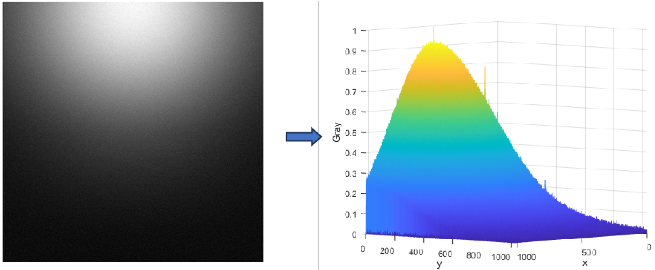
In the equation, $I_{ A,s}$ denotes the radiation intensity of atmospheric scattered light, $I_s$ represents the solar radiation intensity, $\theta$ is the scattering angle, $\gamma \left(\theta \right)$ is the phase function, and l is the scattering path length. $T\left(l\right)$ is the transmission coefficient. Because solar radiation intensity is constant, the radiation intensity of atmospheric scattered light is determined solely by the scattering angle and path length. As a result, the intensity of terrestrial glow impacting star point imaging is affected by both the scattering angle and the scattering route length.

Geometric relationships show that within a local pixel neighborhood, the scattering path length of the terrestrial light in the atmosphere varies continuously and monotonically. Because the fluctuation in the scattering path length is substantially smaller than the overall route length, it is reasonable to assume that the scattering path length along the x and y directions of the star field varies linearly. As a result, a plane model can be used to estimate the scattering path length of light in the atmosphere within the immediate area. A background grayscale model for the immediate region can be created using the linear connection between the incident light intensity and the pixel imaging gray scale in a star sensor.

$$G(x,y)=K{I}_{ A,s}(x,y)+G_0$$

(3)

In the equation, $G(x,y)$ represents the grayscale value of the pixel, K is a constant proportional coefficient determined by the star sensor’s hardware parameters, $I_{ A,s}(x,y)$ denotes the terrestrial glow radiation model from the previous equation, and $G_0$ is the initial background grayscale value.

When the sun approaches the sun sensor’s baffle avoidance angle, solar straylight noise can have a substantial impact on the star sensor’s operation. The windows around the star image point are all small. Within this narrow range, the energy distribution of solar straylight can be modeled as simple linear ramp noise. The collected energy of the pixels $E\left(x,y\right)$ is the sum of a constant threshold and the ramp function, represented as [30].

$$E\left(x,y\right)=e\left(x,y\right)+\mu +k_{1}x+k_{2}y+b$$

(4)

In the equation, $k_1$ and $k_2$ are the slopes in the row direction (x-direction) and column direction (y-direction), respectively; $\mu$ is the background energy threshold; b is the y-intercept of the ramp; and $e\left(x,y\right)$ represents the effective starlight energy value of the pixel.

The centroid truth value $(x_0,y_0)$ is located on a pixel, and its integral coordinate is $(i_{ 0},j_{ 0})$, which is the geometric center point of the pixel, and the window is opened around $(i_{ 0},j_{ 0})$, and the truth offset relative to the pixel center point is defined as ${\beta }_x$ and ${\beta }_y$$({\beta }_x=x_0-i_0,{\beta }_y=y_0-i_0)$, and then the centroid line coordinates (x and y are equivalent) under the background of solar straylight.

2.2. Simulated Star Map

The field of view of the star tracker is 15° × 15°, with a resolution of 1024 × 1024 pixels and a pixel size of 0.008 mm. The simulated star maps are generated using a Hipparcos2 star catalog that includes stars with magnitudes of less than 6.5 Mv. In simulated star maps, noise interference is classified into two types: (1) readout noise from the star sensor’s system, which includes dark current noise, shot noise, photon shot noise, and thermal pixel noise, and (2) strong straylight, which includes sun straylight, moon straylight, and Earth-atmosphere straylight. The star maps obtained under strong straylight interference, after accounting for the aforementioned straylight models and the star sensor’s inherent system noise, are presented below. Figure 2 exhibits the star map Earth-atmosphere straylight interference, Figure 3 depicts the star map under solar straylight interference, and Figure 4 depicts the star map under both sun and moon straylight interference.

2.3. Saliency Detection Algorithm

The star point extraction algorithm suggested in this chapter, which is based on multi-directional gradient local contrast enhancement, is principally inspired by the saliency detection MPCM algorithm. As a result, the purpose of this section is to describe how the MPCM algorithm works. The classic local contrast algorithm (LCM), first proposed by Chen, is a weak target identification algorithm designed for the human vision system. The LCM algorithm calculates each pixel’s local contrast value by discriminating between the weak target region and the background region and then comparing each pixel with its neighbors. 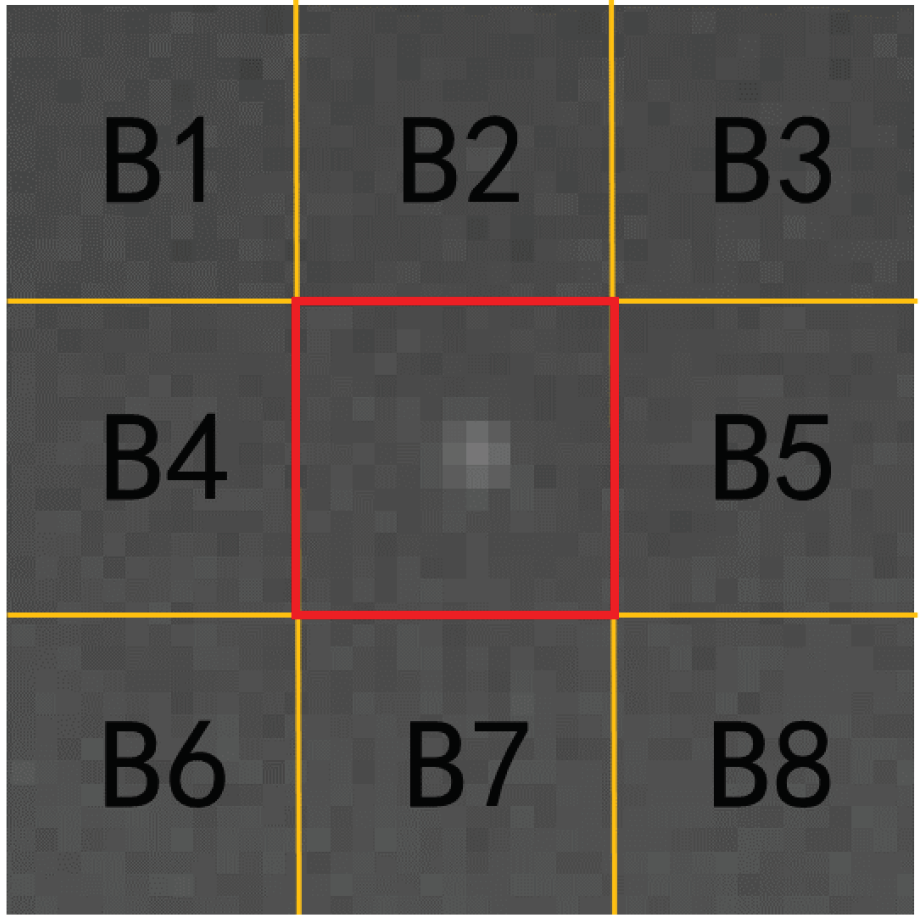Figure 5 shows the definitions for the target and background regions. Here, w represents the current frame image, u denotes the target region, and v signifies the moving scanning window within the image.

Figure 6 depicts the LCM algorithm, which uses a sliding window to travel pixel by pixel across the image from left to right and top to bottom. Each window is divided into 9 (3 × 3) sub-windows, with the middle red rectangular position representing the target’s likely location. Figure 6 depicts the region dividing method used to perform local contrast calculations.

First, calculate the maximum grayscale value $L_0$ at the central region “0”, as follows:

$$L_0=max{I}_k^0, k=1,2,3\dots N$$

(5)

In the equation, $I_k^0$ represents the grayscale value of the k pixel in region 0, and N denotes the number of pixels within the region.

Next, for the eight surrounding small regions (1 to 8) near the central region “0”, calculate the average grayscale value for each of these small regions, as follows:

$$m_i={\displaystyle \frac{1}{N_i}}\sum _k{I}_k^i,k=1,\dots ,N_i,i=1,2,3\dots 8$$

(6)

In the equation, $I_k^i$ represents the grayscale value of the k pixel in the i small region among the eight neighboring regions, while $N_i$ denotes the total number of pixels in the i small region.

Therefore, the contrast value $C_i$ for the central small region and each of the neighboring small regions can be obtained as follows:

$$C_i={\displaystyle \frac{L_0}{m_i}}$$

(7)

Finally, the local contrast LCM value C can be computed as follows:

$$C=mi{n}_i{L}_0\times C_i=mi{n}_i{L}_0\times {\displaystyle \frac{L_0}{m_i}}=mi{n}_i{\displaystyle \frac{L_0^2}{m_i}}={\displaystyle \frac{L_0^2}{ma{x}_i\left(m_i\right)}}$$

(8)

The larger the value of C, the greater the likelihood that the central region contains the target. The analysis is as follows: If the central region is the target, then ${\displaystyle \frac{L_0}{m_i}}>1$, which results in $C=L_0\times {\displaystyle \frac{L_0}{m_i}}>L_0$. If the central region is not the target, then ${\displaystyle \frac{L_0}{m_i}}\le 1$, which results in $C=L_0\times {\displaystyle \frac{L_0}{m_i}}\le L_0$.

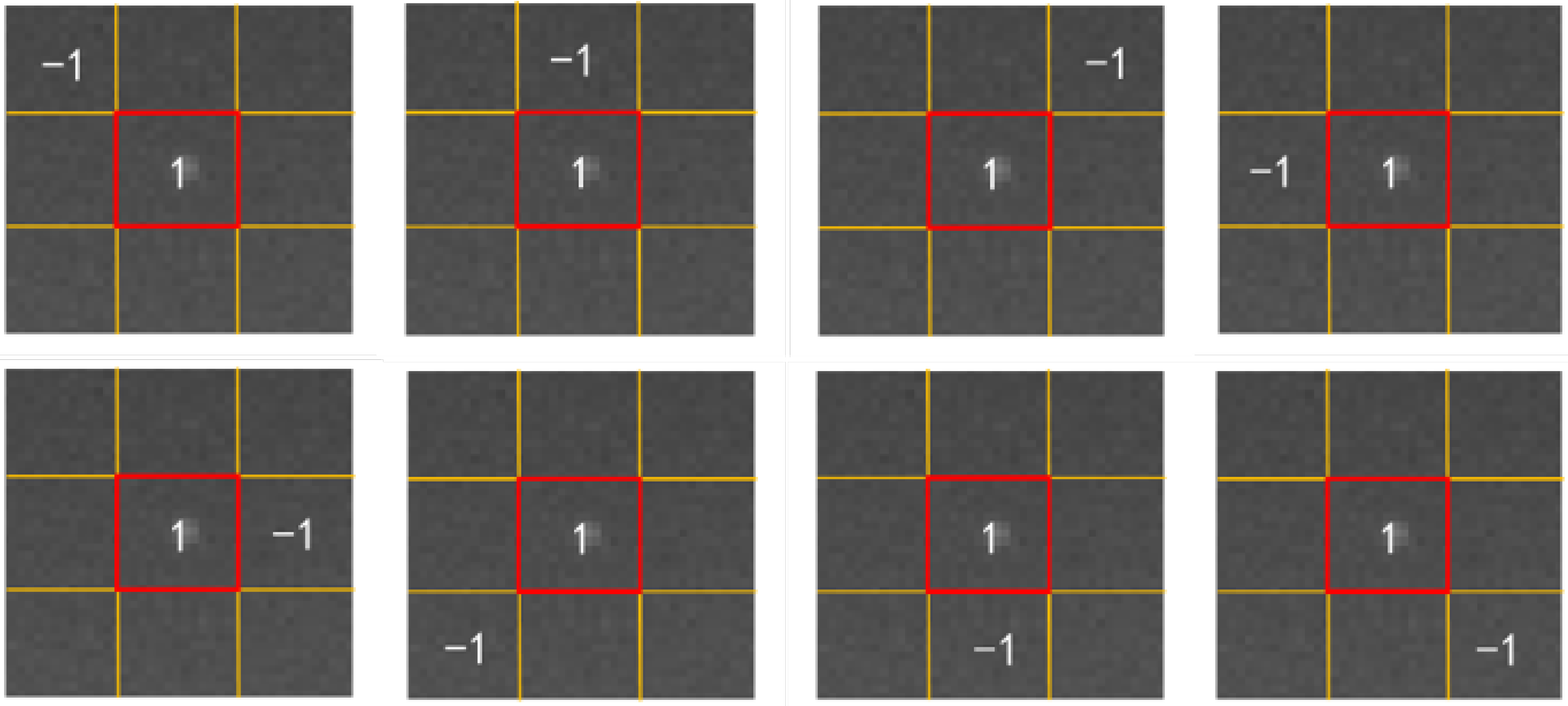
In the PCM(Possibilistic C-means) algorithm, to define the proposed measure, a nested structure is illustrated as shown in Figure 7. First, the sliding window is divided into two parts: the center red rectangular box, denoted as T, where the target is likely to appear, and the surrounding part, which represents the background. To measure local contrast more accurately, the surrounding background part is divided into 8 patches $Bi$, where $i=1,2,3,\dots ,8$. This method aims to enhance the target and suppress the background. The definition of the PCM algorithm is as follows:

The difference between the target sub-window T and the background sub-window $Bi$ can be defined as follows:

$$D\left(T\right)=\left(\begin{array}{c}d(T,B1)\\ d(T,B2)\\ ⋮\\ d(T,B8)\end{array}\right)$$

(9)

In the equation, d represents the degree of difference between the target and the background. There are various methods for calculating d; this paper uses the mean difference method as follows:

$$d(T,Bi)=m_T-m_{Bi},(i=1,2,\dots ,8)$$

(10)

In the equation, $m_T$ and $m_{Bi}$ represent the mean pixel values of the target region and the background sub-region, respectively.

Building on the above, a local contrast measure at a certain scale is further introduced to effectively describe the prominence of small targets in complex backgrounds. For small targets, the grayscale intensity within the region often differs significantly from the surrounding background. To quantitatively describe this property, this paper proposes the following definition:

$${\tilde{d}}_i=d(T,Bi)\ast d(T,Bi+4),(i=1,2,\dots ,4)$$

(11)

In the equation, ${\tilde{d}}_i$ indicates the difference between the reference patch and the background patch in the i direction. We can see that when $d(T,Bi)$ and $d(T,Bi+4)$ have the same sign, ${\tilde{d}}_i>0$. This means that the intensity of the central putative target region is either greater or less than that of the background patches. As a result, it can be used to assess the properties of the target region.

In dim target enhancement, the contrast between the target and background regions should be as high as possible. Figure 8 shows the minimal distance between the reference sub-window and the surrounding background sub-window, which can be used to measure contrast. To calculate a sub-window-based contrast measure (PCM) on a given scale, follow these steps:

$${\mathcal{C}}_{(x_{ii},y_{jj})}=\underset{i=1,2,3,\dots ,4}{min}{\tilde{d}}_i$$

(12)

where $(x_{ii},y_{jj})$ represents the coordinates of the reference center pixel.

$$m_T={\displaystyle \frac{1}{N\times N}}\underset{i=x_{ii}-floor(N/2)}{\sum ^{x_{ii}+floor(N/2)}}\underset{j=y_{ii}-floor(N/2)}{\sum ^{y_{ii}+floor(N/2)}}f(x_i,y_j)$$

(13)

where N is the width and height of the image, and $floor(N/2)$ rounds $N/2$ down to the nearest integer less than or equal to $N/2$. The PCM algorithm workflow is as follows:

(1) Calculate the mean grayscale value of the target sub-window.

$$m_T={\displaystyle \frac{1}{N\times N}}\underset{i=x_{ii}-floor(N/2)}{\sum ^{x_{ii}+floor(N/2)}}\underset{j=y_{ii}-floor(N/2)}{\sum ^{y_{ii}+floor(N/2)}}f(x_i,y_j)$$

(14)

(2) Apply the 8 filters, as shown in the figure, to each background sub-window to obtain the background-reduced image.

(3) Compute the local contrast of the image using the following formula:

$${\tilde{d}}_i=d(T,Bi)\ast d(T,Bi+4),(i=1,2,\dots ,4)$$

(15)

(4) Slide the window across the entire image until the whole image is processed, and output the saliency contrast map C, calculated using the following formula:

$${\mathcal{C}}_{(x_{ii},y_{jj})}=\underset{i=1,2,3,\dots ,4}{min}{\tilde{d}}_i$$

(16)

In practical applications, the size of small targets is often not predetermined. Therefore, the window size should be as close as possible to the actual size of the small target. According to the definition of the MPCM algorithm, the calculation formula is as follows:

$$\widehat{C_{p,q}}=\underset{l=1,2,\dots L}{max}{C}^l(p,q)$$

(17)

where $C^l$ represents the local contrast map at multiple scales, with l indicating different scales of the sub-window, L being the maximum scale, and p and q representing the number of rows and columns in the contrast map, respectively.

From the definition of MPCM, it is clear that it is straightforward and suitable for parallel computation. From the above formula, if $d(T,Bi)>0$ for all i in the target region, then T is a bright target; otherwise, T is a dark target. Based on this property, MPCM has two special cases. If only bright targets are present in the known application scenario, then it is as follows:

$${\tilde{d}}_i=\left\{\begin{array}{cc}d(T,Bi)\ast d(T,Bi+4)& \mathrm{if}d(T,Bi)>0\mathrm{and}d(T,Bi+4)>0)\\ 0& \mathrm{otherwise},\end{array}\right.$$

(18)

where $i=1,2,3,4$. Similarly, the following formulas can be derived for dark targets:

$${\tilde{d}}_i=\left\{\begin{array}{cc}d(T,Bi)\ast d(T,Bi+4)& \mathrm{if}d(T,Bi)<0\mathrm{and}d(T,Bi+4)<0)\\ 0& \mathrm{otherwise},\end{array}\right.$$

(19)

MPCM can benefit both bright and dark targets. Using the MPCM algorithm, a mean filtering operation can be used as a preprocessing step. This procedure serves to successfully suppress visual clutter and noise, enhancing target recognition accuracy. Mean filtering smoothes out the image, lessening the effect of local noise on future processing. This enables the MPCM algorithm to more accurately identify target regions in complicated backdrops. The MPCM algorithm’s primary role in target detection is to increase the saliency of the target region while suppressing background interference. Because the target zone is brighter than the background, MPCM can improve its brightness attributes at various scales. This enhancement makes the target more visible in the image, increasing the accuracy of target detection. When $d(T,Bi)$ and $d(T,Bi+4)$ have opposite signs, the contrast drops. When $d(T,Bi)$ and $d(T,Bi+4)$ have the same sign, we have

$$C_{(x_{ii},y_{jj})}=\underset{i=1,2,3,4}{min}{\tilde{d}}_i=\underset{i=1,2,3,4}{min}d(T,Bi)\ast d(T,Bi+4)\ge d{(T,B\tilde{i})}^2={(T-m_{\tilde{i}})}^2$$

(20)

$$f\left(T\right)={(T-m_{\tilde{i}})}^2$$

(21)

$$f^{\prime }\left(T\right)=2(T-m_{\tilde{i}})$$

(22)

From the formula, it is clear that the larger T is, the greater $f\left(T\right)$ becomes. This means that when T is a target, the contrast value increases significantly. Conversely, when T is background, it resembles the surrounding module. In this case, the contrast approaches zero, indicating that the method can enhance the target while suppressing the background.

2.4. Star Point Centroid Calculation

2.4.1. Star Map Enhancement

Although a star field is composed of discrete pixels in a two-dimensional space, due to the relative continuity of pixel grayscale values in the local area, the star field can typically be considered as a two-dimensional surface. In the theory of differential calculus for single-variable functions, curvature is often used to represent the degree of bending of a point on a surface. Suppose that there is a point $\mathrm{T}(x,y(x\left)\right)$ on the surface y, and this point $\mathrm{T}(x,y(x\left)\right)$ has second-order derivative characteristics. The curvature of this point on the surface can be expressed as

$$\left\{\begin{array}{c}{G}_x(x,y)={\displaystyle \frac{I(x+1,y)-I(x-1,y)}{2}}\\ G_y(x,y)={\displaystyle \frac{I(x,y+1)-I(x,y-1)}{2}}\end{array}\right.$$

(23)

$$y^{\prime }(x,y)=\sqrt{G_x{(x,y)}^2+G_y{(x,y)}^2}$$

(24)

where $G_x(x,y)$ is the horizontal gradient of pixel point $(x,y)$, $G_y(x,y)$ is the vertical gradient of pixel point $(x,y)$, and $y^{\prime }(x,y)$ is the first derivative of pixel point $(x,y)$.

$$\left\{\begin{array}{c}{G}_{xx}(x,y)=I(x+1,y)-2I(x,y)+I(x-1,y)\\ G_{yy}(x,y)=I(x,y+1)-2I(x,y)+I(x,y-1)\end{array}\right.$$

(25)

$$G_{xy}(x,y)={\displaystyle \frac{I(x+1,y+1)-I(x+1,y-1)-I(x-1,y+1)+I(x-1,y-1)}{4}}$$

(26)

$$y^{″}(x,y)=\sqrt{G_{xx}^2+G_{yy}^2+2G_{xy}^2}$$

(27)

where $G_{xx}(x,y)$ is the second derivative of the horizontal direction of pixel point $(x,y)$, $G_{yy}(x,y)$ is the second derivative of the vertical direction of pixel point $(x,y)$, $G_{xy}(x,y)$ is the second derivative of the mixed direction of pixel point $(x,y)$, and $y^{″}(x,y)$ is the second derivative of pixel point $(x,y)$.

$$S={\displaystyle \frac{|y^{″}|}{{(1+y^{\prime 2})}^{\frac{3}{2}}}}$$

(28)

where S represents the curvature value at the point $\mathrm{T}(x,y(x\left)\right)$, $y^{″}$ denotes the second-order derivative at this point on the surface, and $y^{\prime }$ represents the first-order derivative at this point on the surface.

The curvature of a point on an image can be represented as a combination of the second-order and first-order derivatives in a certain direction on the surface at that point. Considering the discrete nature in the digital domain, the spatial curvature at a point on the image can be comprehensively represented using the first-order and second-order derivative values in four directions: 0°, 90°, 180°, and 270°.

In this paper, the facet model proposed by Haralick is used to describe the star field. First, let R = {−2, −1, 0, 1, 2} and C = {−2, −1, 0, 1, 2} be the index sets for symmetric neighborhoods. The pixel values within a 5 × 5 neighborhood can be used to represent the current center pixel, and can be expressed by the following formula:

$$f(r,c)=\underset{i=1}{\sum ^{10}}{Q}_i{B}_i(r,c)$$

(29)

where $B_i(r,c)$ represents the discrete orthogonal polynomial basis, and $(r,c)$ satisfies $(r,c)\in R\times C$.

$$\left\{B_i(r,c)\right\}=\left\{1,r,c,r^2-2,rc,c^2-2,r^3-\left({\displaystyle \frac{17}{5}}\right)r,(r^2-2)c,r(c^2-2),c^3-\left({\displaystyle \frac{17}{5}}\right)c\right\}$$

(30)

where $Q_i$ represents the combination coefficient, and each combination coefficient $Q_i$ for a pixel $(x,y)$ in the star field is unique. Therefore, the expression for the combination coefficient $Q_i$ can be obtained using the least squares fitting of the polynomial orthogonality characteristics, as follows:

$$Q_i=\sum _r\sum _c{\displaystyle \frac{f(r,c)B_i(r,c)}{{\displaystyle \sum _r}{\displaystyle \sum _c}{B}_i^2(r,c)}}$$

(31)

A portion of the variables can be represented using the weight coefficient $W_i$, as follows:

$$W_i=\sum _r\sum _c{\displaystyle \frac{B_i(r,c)}{{\displaystyle \sum _r}{\displaystyle \sum _c}{B}_i^2(r,c)}}$$

(32)

Thus, the combination coefficient $Q_i$ can be expressed as

$$Q_i=f(r,c)\ast W_i$$

(33)

where the combination coefficient $Q_i$ is represented by the convolution of the weight coefficient $W_i$ and the star field, with the weight coefficient $W_i$ determined based on the characteristics of $B_i(r,c)$.

Combining the principles of directional derivative calculation, the first-order and second-order derivatives of the pixel $(x,y)$ along the direction vector $\gamma$ can be expressed as

$${\displaystyle \frac{\partial f}{\partial \gamma }}{|}_{(x,y)}=\left(\begin{array}{c}{Q}_2-{\displaystyle \frac{17}{5}}{Q}_7-2Q_9\end{array}\right)sin\alpha +\left(\begin{array}{c}{Q}_3-{\displaystyle \frac{17}{5}}{Q}_{10}-2Q_8\end{array}\right)cos\alpha$$

(34)

$${\displaystyle \frac{{\partial }^{2}f}{\partial {\gamma }^2}}{\mid }_{(x,y)}=2Q_{4}si{n}^2\alpha +2Q_{5}sin\alpha cos\alpha +2Q_{6}co{s}^2\alpha$$

(35)

where $\alpha$ represents the angle between the direction vector $\gamma$ and the horizontal direction of the image.

The preceding formula demonstrates that the computing cost of the second-order derivative is lowered from O(2N) to O(N) when compared with the first-order derivative. As a result, in the following methods provided in this work, only the second-order derivative will be employed to represent the image’s curvature information.

Local contrast enhancement is conducted on the star points in the star field using the second-order derivatives derived at angles of 0°, 90°, 180°, and 270°. The goal of local contrast enhancement is to emphasize the properties of the star points while minimizing interference from complicated backgrounds. Prior to local contrast augmentation, a feature analysis of the star points’ second-order derivatives is performed.

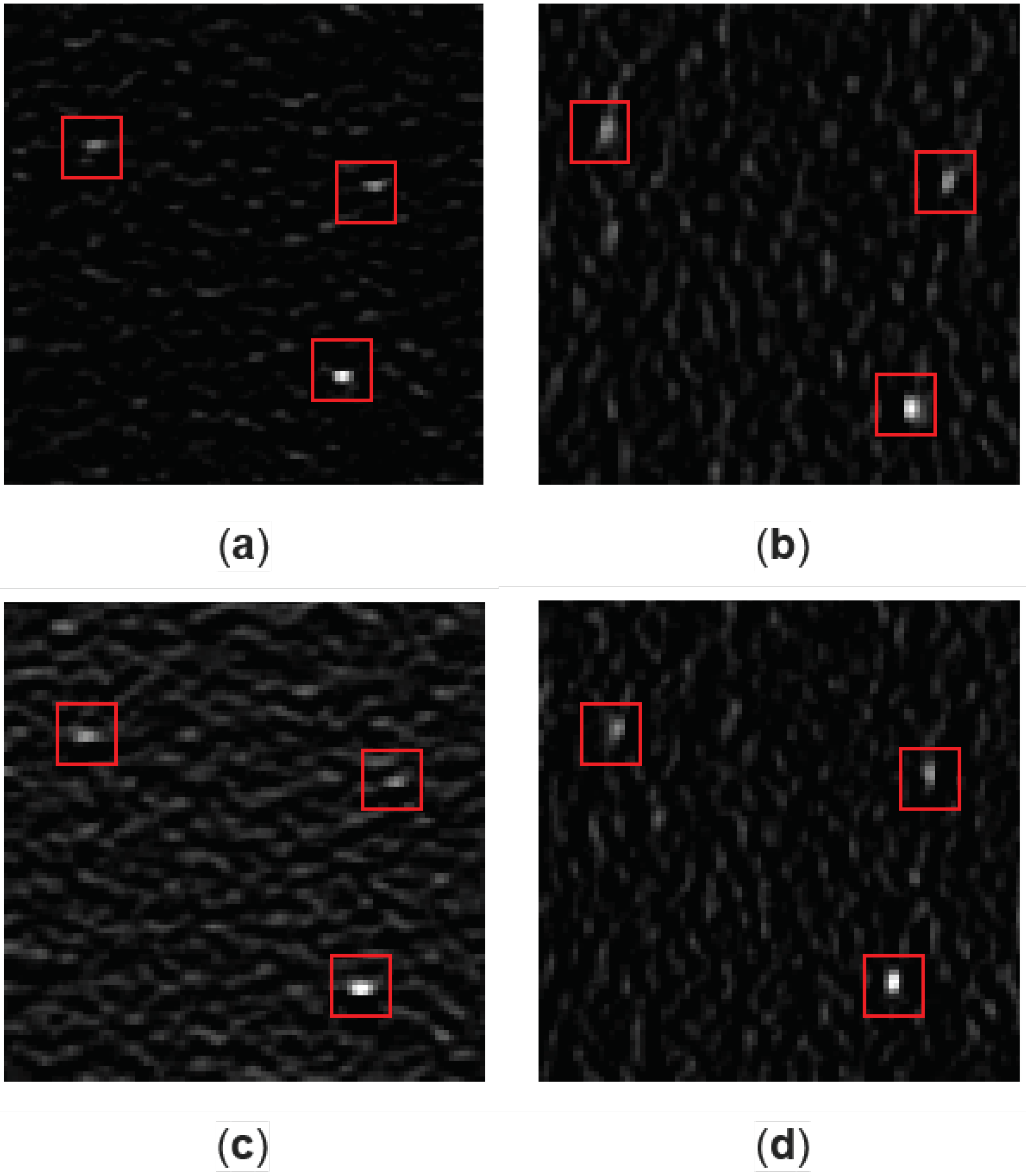
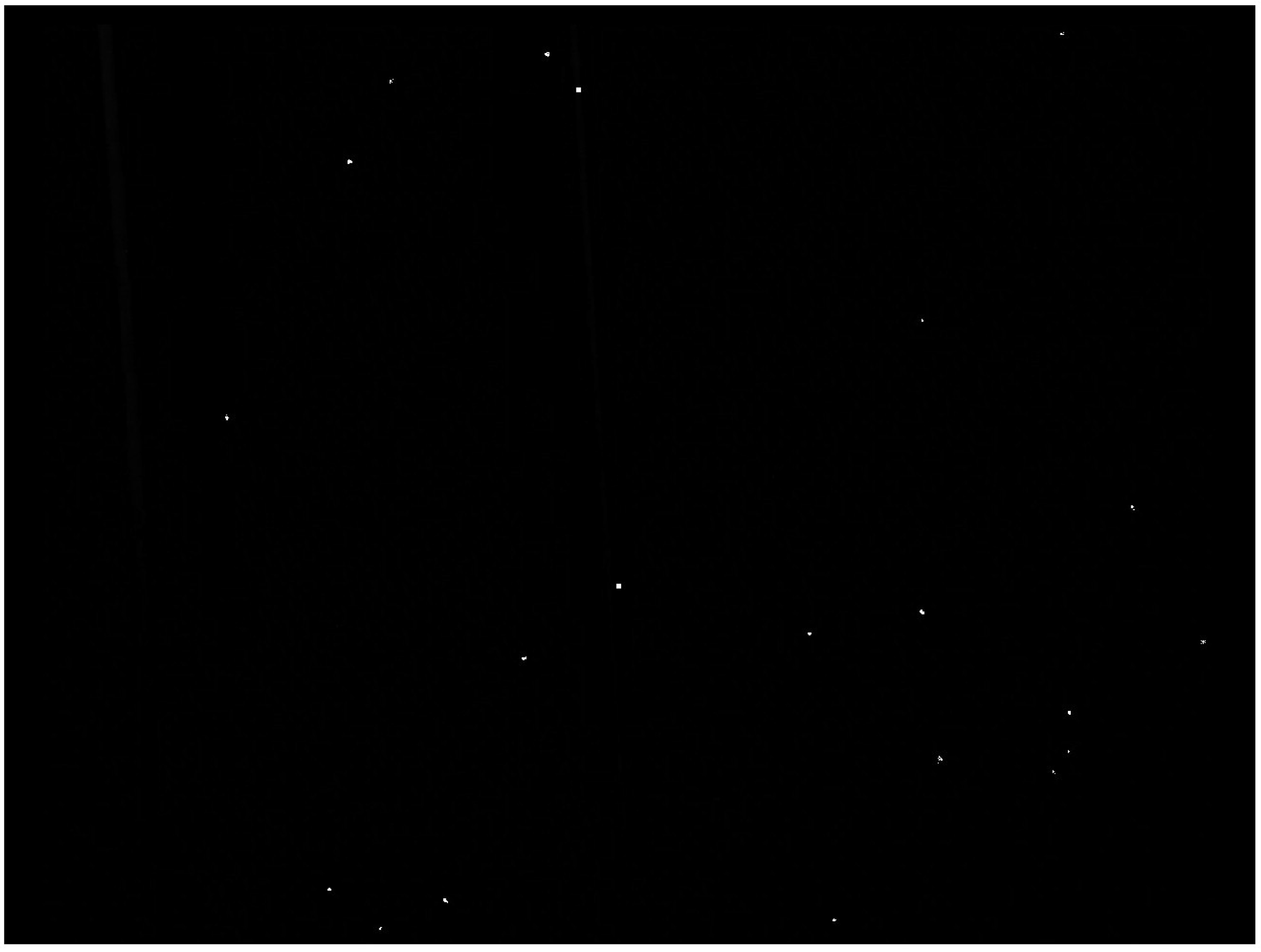
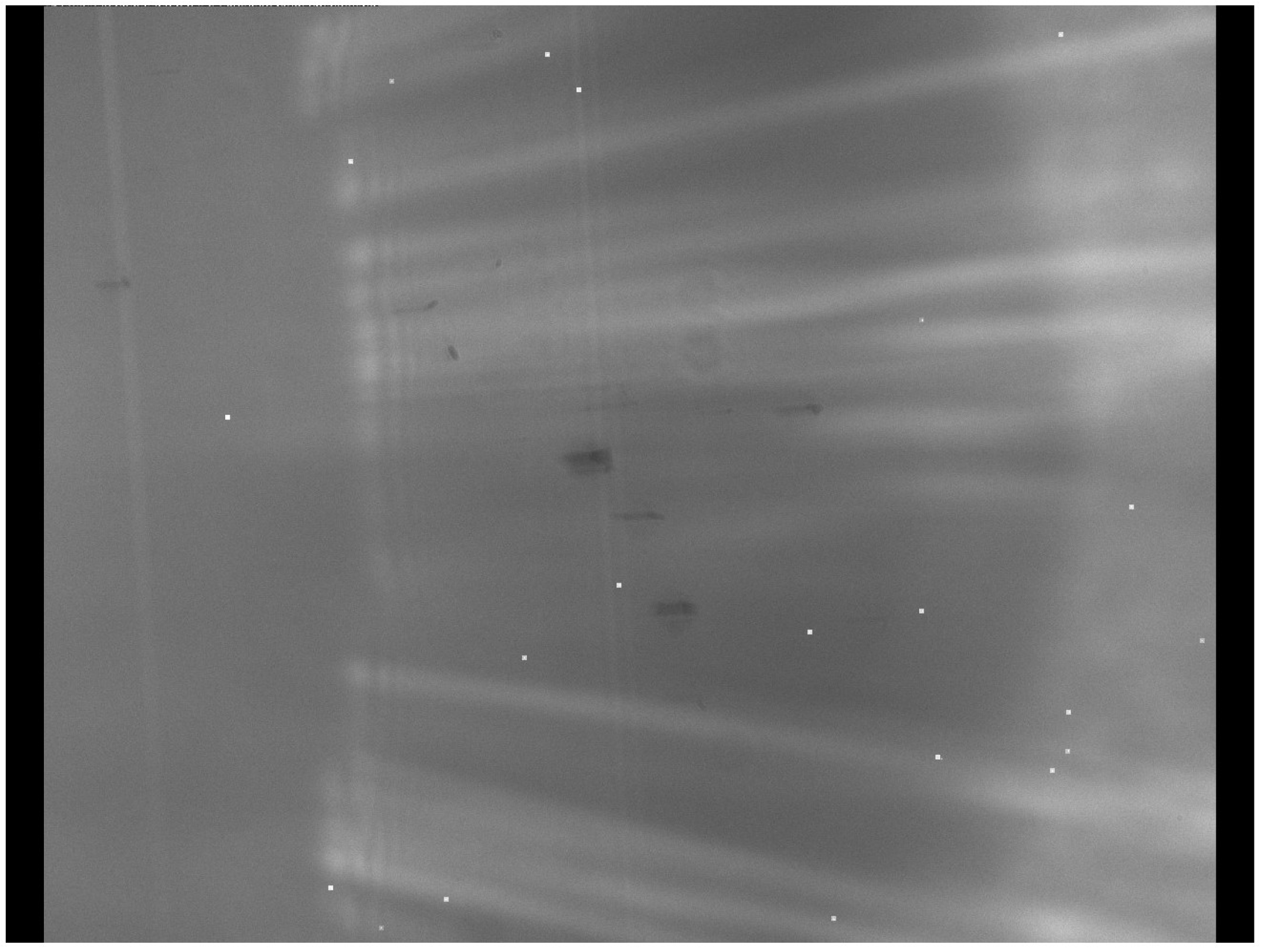
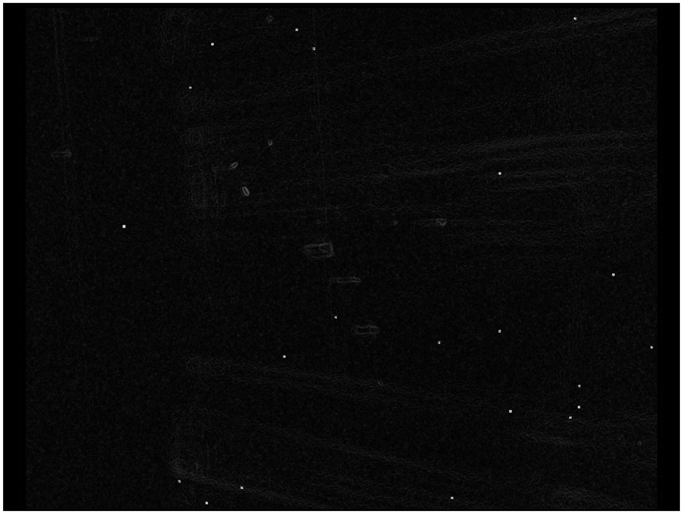
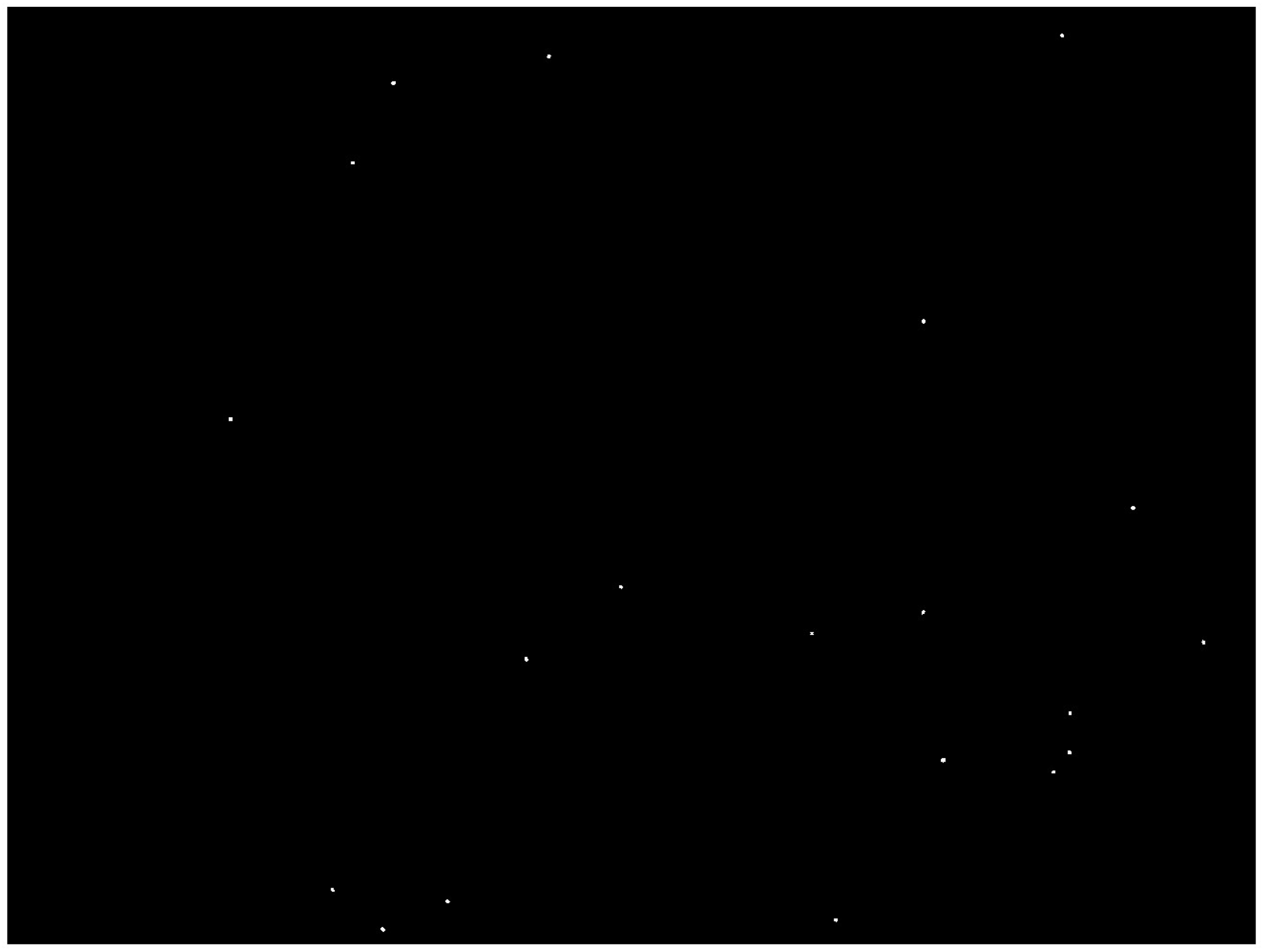
Figure 9 shows the local star field processed using second-order derivatives in the 0°, 90°, 180°, and 270° directions, top to bottom and left to right. In the red rectangle box is a partial enlarged image of the star points after gradient enhancement. The graphic clearly shows that the directional second-order derivative approach improves the local star field while efficiently suppressing interference from intense straylight. Each augmented star field image significantly improves the visibility of star points in all four directions, facilitating the implementation of following star point identification algorithms. Furthermore, this approach remains robust in the presence of significant straylight contamination, which is typical in astronomical photography. It increases not just the visibility of star points but also the overall quality of the star field by decreasing unwanted noise interference.

To address the concerns raised, we offer an improved star point centroid localization approach designed specifically for star maps influenced by severe straylight interference. The suggested method begins with a multi-directional gradient improvement of the star map, which successfully mitigates the effects of intense straylight. Figure 10 shows how gradient images of the star map in four directions—0°, 90°, 180°, and 270°—are combined to create a locally enhanced star map. This multi-directional gradient enhancement increases the prominence of the star points, which improves their detection capabilities.

2.4.2. Star Detection

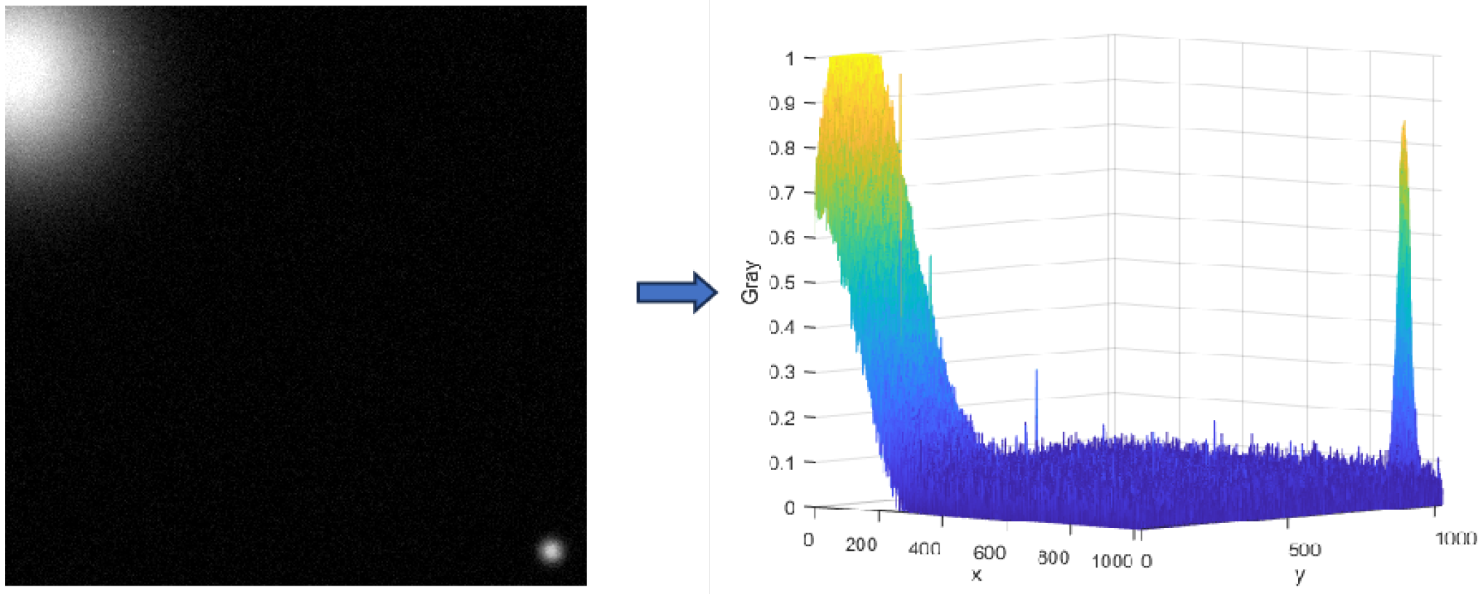
Currently, local contrast enhancement algorithms based on the human visual system can successfully extract faint star points that are difficult to separate from background noise, considerably enhancing star point identification capabilities. However, these techniques continue to face hurdles in actual applications requiring high-precision centroid localization of star points. Although dim star points can be effectively retrieved, their energy distribution patterns are frequently disturbed, making precise centroid extraction challenging. 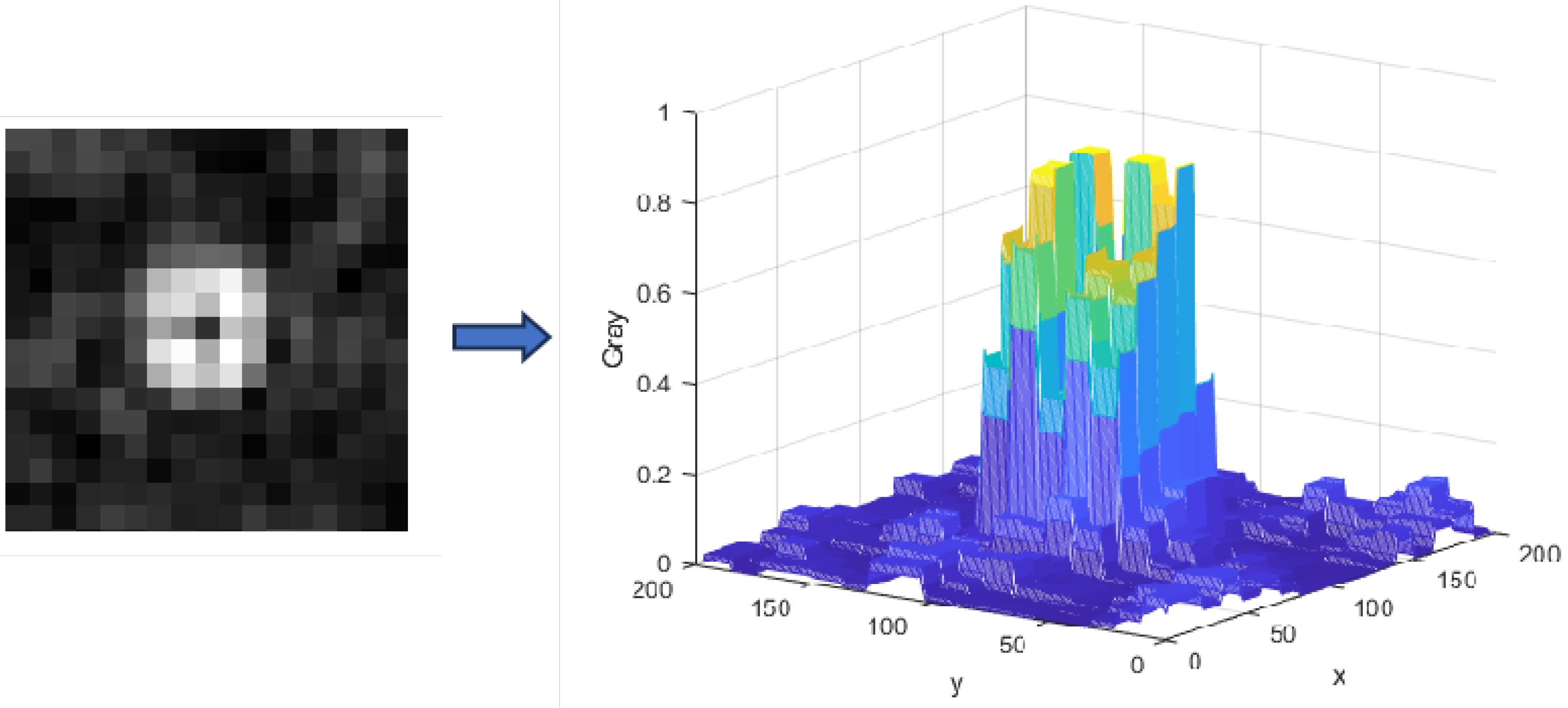As illustrated in Figure 11, the overemphasis on local information during the execution of local contrast enhancement algorithms can result in irregular energy distributions of star points, upsetting their original distribution. This disturbance not only alters the overall form of the star points, but also complicates and makes the subsequent centroid extraction process more complex. Centroid extraction, an important step in star point analysis, has a substantial impact on subsequent star point analysis and categorization.

In the enhanced star map, the MPCM algorithm is used for initial star point extraction. By performing connected component analysis on the enhanced star map and combining it with threshold segmentation, noise is effectively filtered out, and coarse localization of the star points is achieved.

2.4.3. Star Point Centroid Localization

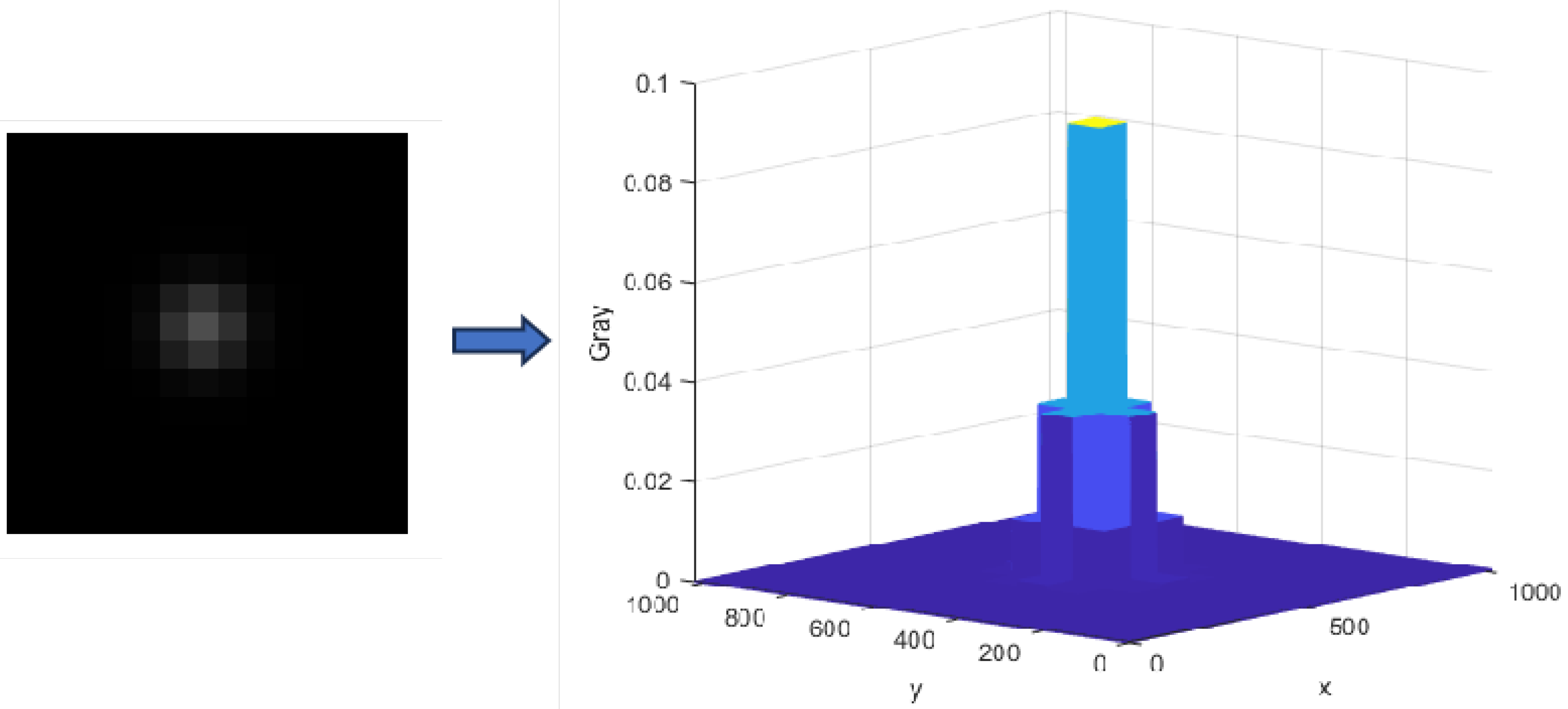
As illustrated in Figure 12, the intensity distribution of an initial star point imaged on a star tracker is obtained by convolving the intensity distribution function with the optical system’s point spread function. In the ideal model, the star is considered a point target. To achieve higher centroid localization accuracy, the optical system of the star tracker often employs defocusing methods to spread the star spots on the imaging surface to a range of 3 × 3 to 5 × 5 pixels [31].

$$I\left(x,y\right)={\displaystyle \frac{I_0}{2\pi {{\sigma }^2}_{psf}}}exp\left[-{\displaystyle \frac{{\left(x-x_c\right)}^2+{\left(y-y_c\right)}^2}{2{{\sigma }^2}_{psf}}}\right]$$

(36)

where $I_0$ is the total energy of the star radiated to the imaging plane during the camera exposure time, $\left(x_c,y_c\right)$ denotes the coordinates of the star’s center on the imaging plane, and ${\sigma }_{psf}$ represents the diffusion radius of the Gaussian point spread function, indicating the concentration of the star image’s energy.

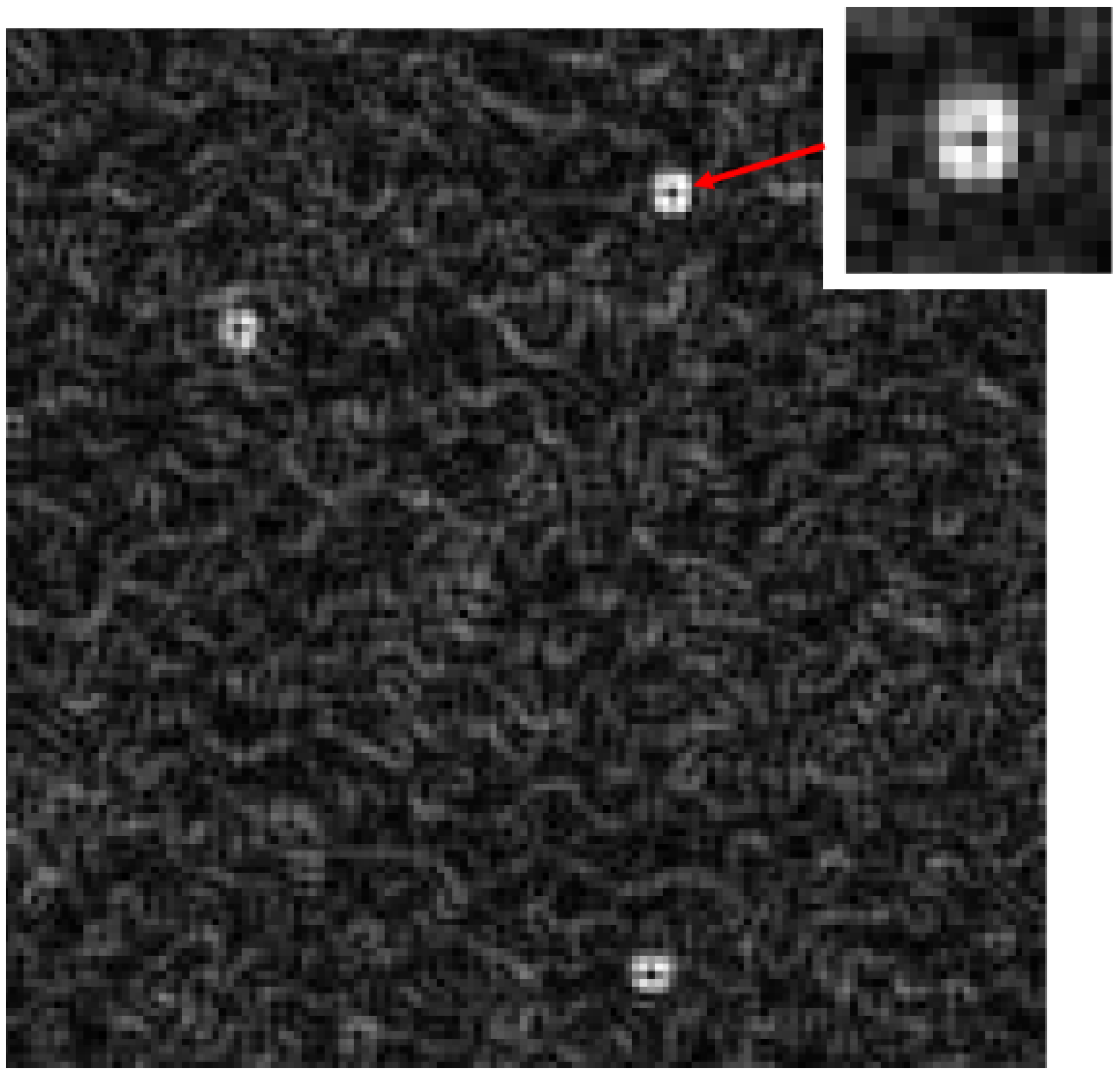
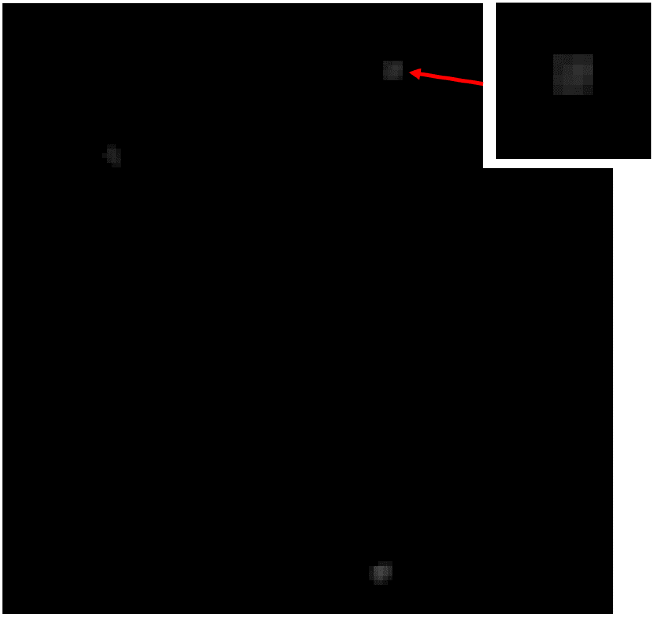
As shown in Figure 13, the enhanced star map has an energy distribution pattern with low intensity in the center and high intensity at the edges, which can be approximated as a Gaussian-like distribution near the starting star point. However, due to camera system noise and significant straylight noise, the energy distribution of the improved star map may be compromised to some extent.

In order to overcome this problem, we process the 3 × 3 pixel neighborhood around each star point. As shown in the following formula, the gray values in the eighth neighborhood of the pixel with the lowest energy are arranged from small to large ($G_i(i=1,2,3\dots ,8)$), and the variance of the pixels in the eighth neighborhood is calculated. The maximum gray value and the sub-maximum gray value in the eighth neighborhood are subtracting variance. The minimum gray value and the sub-small gray value plus variance can reduce the influence of noise on centroid calculation and improve the accuracy of star centroid localization.

$$\left\{\begin{array}{c}{G}_8^{\prime }=G_8-G_{Var}\hfill \\ G_7^{\prime }=G_7-G_{Var}\hfill \\ G_2^{\prime }=G_2+G_{Var}\hfill \\ G_1^{\prime }=G_1+G_{Var}\hfill \end{array}\right.$$

(37)

In the equation, $G_{Var}$ is the variance of the eighth neighborhood; $G_8$, $G_7$, $G_8^{\prime }$, and $G_7^{\prime }$ are respectively the maximum gray value in the eighth neighborhood, the sub-major gray value, the maximum gray value after compensation, and the sub-major gray value after compensation; and $G_1$, $G_2$, $G_1^{\prime }$, and $G_2^{\prime }$ are respectively the minimum gray value in the eight neighborhood, the sub-small gray value, the minimum gray value after compensation, and the sub-small gray value after compensation.

This method integrates the star point’s energy distribution characteristics and noise compensation strategy, significantly enhancing the accuracy and reliability of star point detection under strong straylight interference.

Gaussian fitting, the weighted centroid approach, and the threshold-based centroid method are popular algorithms for extracting star centroids [32,33,34,35,36]. The star points after picture enhancement are difficult to fit to compute the center of mass using the Gaussian approach. The weighted centroid approach has low anti-interference ability. The threshold-based centroid method is simple to develop and has excellent anti-noise properties, making it ideal for centroid extraction in this work. As a result, we use the threshold-based centroid approach to calculate centroid values. This approach works by using the gray value of the target pixels within the star picture region to weight their coordinates. The formula for this procedure is provided by

$$\left\{\begin{array}{c}{x}_{\mathrm{e}}={\displaystyle \frac{{\displaystyle \underset{j=r_1}{\sum ^{r_2}}}{\displaystyle \underset{i=c_1}{\sum ^{c_2}}}i{G}^2\left(i,j\right)}{{\displaystyle \sum _{j=r_1}}{\displaystyle \underset{i=c_1}{\sum ^{c_2}}}{G}^2\left(i,j\right)}}-T\\ y_{\mathrm{e}}={\displaystyle \frac{{\displaystyle \underset{j=r_1}{\sum ^{r_2}}}{\displaystyle \underset{i=c_1}{\sum ^{c_2}}}j{G}^2\left(i,j\right)}{{\displaystyle \underset{j=r_1}{\sum ^{r_2}}}{\displaystyle \underset{i=c_1}{\sum ^{c_2}}}{G}^2\left(i,j\right)}}-T\end{array}\right.$$

(38)

In the formula, $\left(i,j\right)$ represents the pixel coordinates; $G\left(i,j\right)$ denotes the pixel gray value; T is the local background threshold for the star point; $(c_1,r_1)$ indicates the coordinates of the top-left pixel of the target star image window; $(c_2,r_2)$ represents the coordinates of the bottom-right pixel of the target star image window, which should encompass all valid pixels covered by the star image point; and $(x_{\mathrm{e}},y_{\mathrm{e}})$ is the estimated value of the star image point’s centroid $(x_0,y_0)$, with subpixel accuracy.

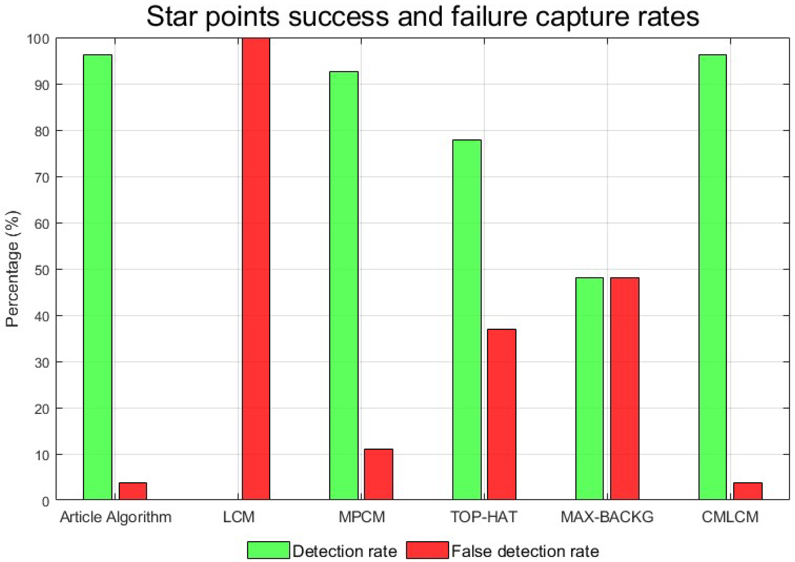
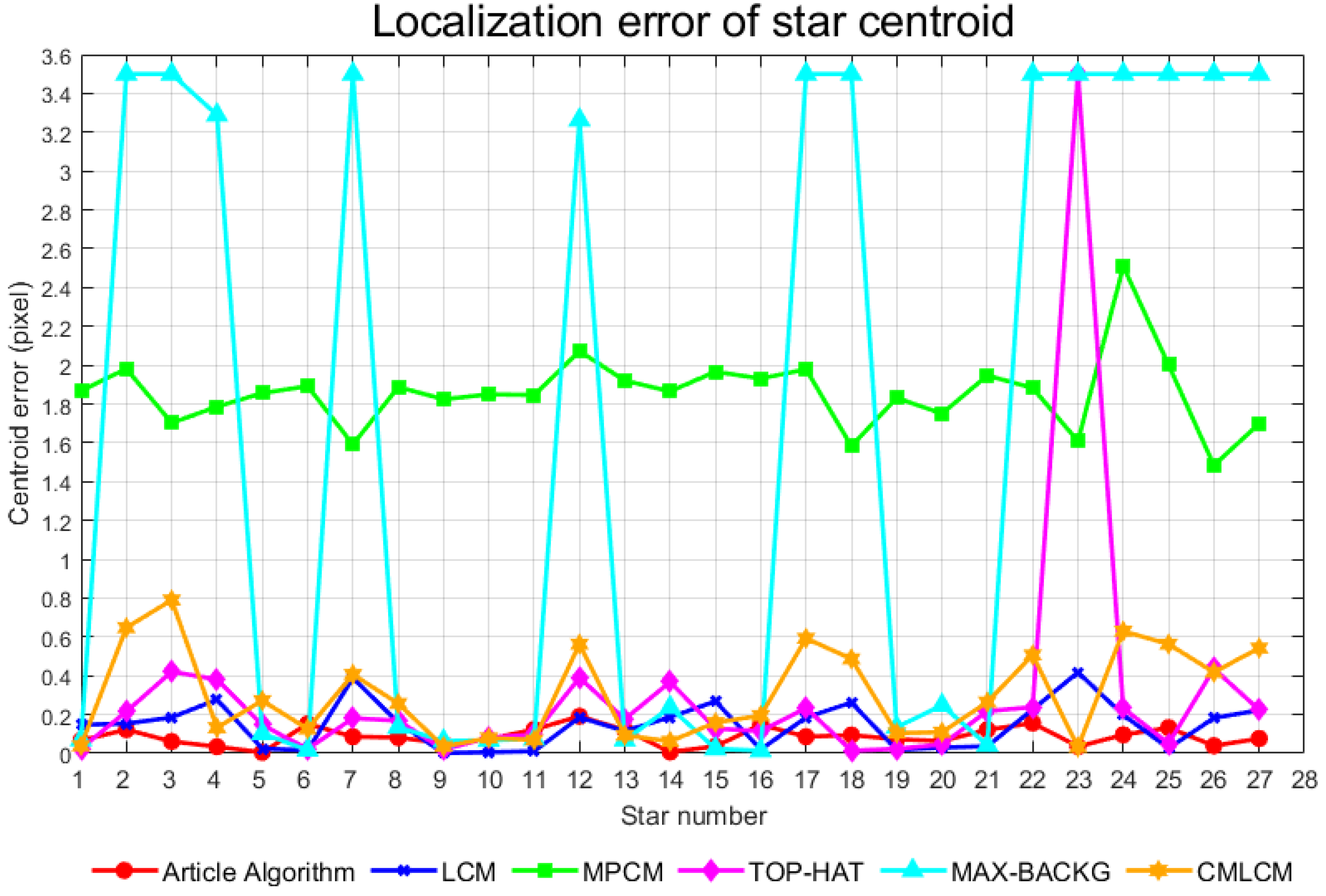
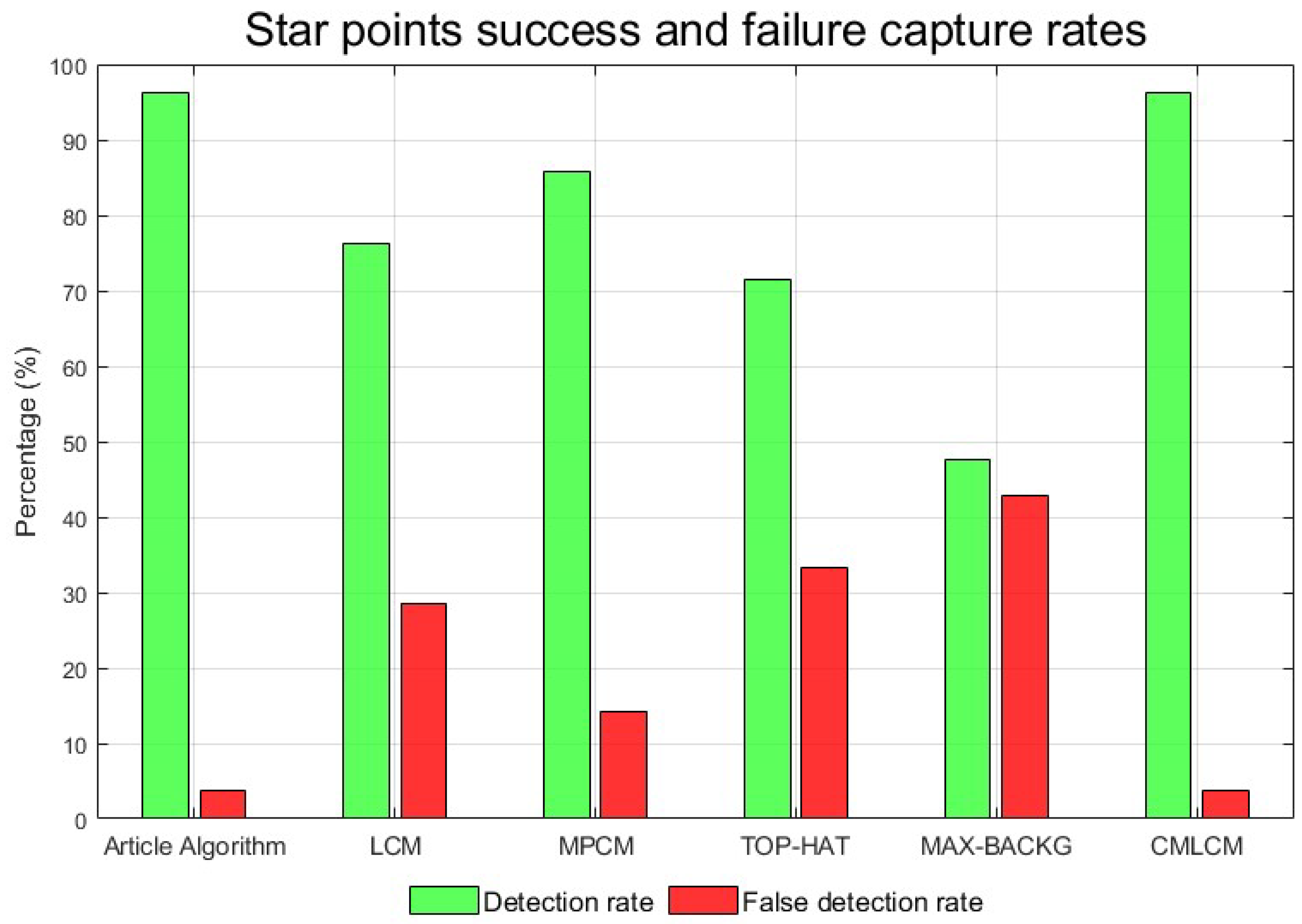
For star maps with strong straylight interference, traditional algorithms (TOP-HAT, MAX-BACKG) rely on accurate background modeling and reasonable processing of the highlighted areas in the image. When straylight introduces a wide range of high-light interference in the image, the two methods may not be able to effectively separate the target and straylight, resulting in poor target recognition or an enhancement effect. Therefore, the algorithm in this paper first introduces a multi-directional gradient to locally enhance the star map under strong straylight interference, enhance the difference degree between the target and the strong straylight background, and improve the subsequent star point extraction rate. Classical significance testing algorithms (LCM, MPCM) are affected by background changes, luminance distribution distortion, and local contrast failure. These problems often lead to inaccurate extraction of salient regions, possibly misinterpreting straylight as the target region, or failing to accurately identify the true target. The CMLCM algorithm first enhanced the image of the star map under the interference of strong straylight, and then extracted the star points directly through the LCM algorithm and threshold segmentation. In this way, the energy distribution of the star points obtained by direct processing was broken, resulting in the low accuracy of star centroid positioning. First, this algorithm makes the enhanced star energy distribution as close as possible to Gaussian distribution by means of four-way gradient local star energy enhancement, and determines the star neighborhood position distribution by the rough extraction of centroid positioning, and introduces the star local neighborhood gray compensation mechanism to further improve the star energy distribution so as to achieve high-precision positioning of a star centroid.

3. Experiment and Analysis

To evaluate the effectiveness and performance of the proposed algorithm under strong straylight interference, and to conduct a comparative analysis with other algorithms, the following algorithms are considered: TOP-HAT, MAX-BACKG, LCM, MPCM, and CMLCM. In the comparison of different algorithms, the first step is to analyze the false alarm rate versus detection rate using Receiver Operating Characteristic (ROC) curves [28]. In the ROC curve, the horizontal axis represents the false detection rate (FD), while the vertical axis represents the detection rate (DR). The star false detection rate is the proportion of noise misidentified as the total number of accurate stars in the star astrological chart. This relationship can be expressed by the following formula:

$$\left\{\begin{array}{c}{p}_d={\displaystyle \frac{N_C}{N_T}}\\ p_f={\displaystyle \frac{N_e}{N_P}}\end{array}\right.$$

(39)

where $N_T$ represents the number of actual star targets in the star map, $N_C$ denotes the number of correctly detected star points, $N_e$ indicates the number of erroneously detected star points, and $N_P$ is the total number of detected targets (including both correctly detected and erroneous star points).

3.1. Simulation Experiment

3.1.1. Experimental Results of Star Detection Rate and False Detection Rate

Figure 14, Figure 15 and Figure 16 show the ROC curves of various algorithms with varying degrees of significant straylight interference. The detection performance of every algorithm varies; however, the suggested algorithm is resilient against diverse straylight impacts. Under the three conditions, the suggested algorithm outperforms most other algorithms in terms of effective and false detection rates. Only the CMLCM algorithm demonstrates detection and false detection rates equivalent to the suggested technique. The proposed algorithm and the CMLCM algorithm achieve a 100% effective detection rate and a 0% false detection rate for star points under both Earth-atmosphere straylight interference and sunlight interference conditions. In contrast, the other four algorithms either fail to fully capture the star points or mistakenly identify noise as star points under these conditions. When both sun straylight and moon straylight interference are present, the proposed algorithm and the CMLCM algorithm both achieve a 96.29% effective star point extraction rate and a 3.70% false detection rate. The classical significance detection algorithm LCM encounters issues with star point capture failure, while the other three algorithms show significant problems with star point detection rates and false detection rates, which could potentially reduce the subsequent star sensor’s star point capture efficiency. Based on the detection rate and false detection rate of star points under the three working conditions, the proposed algorithm maintains high accuracy in detecting effective star points under all three types of strong straylight interference. Furthermore, the number of erroneous star points identified is extremely low, which reduces the possibility of mismatches during subsequent star point identification, boosting the star sensor’s capture speed and success rate.

3.1.2. Experimental Results of Star Centroid Localization

Figure 17 depicts the centroid extraction error curves for various approaches under varying levels of intense straylight interference. The simulated star maps with strong straylight contain a total of 27 effective star points. If a method is unable to extract the centroid for a specific star point, the centroid error is set to the greatest value of the centroid error curve (3.5 pixels).

Based on Figure 17, which shows the centroid error curves, and

Table 1. The root mean square and variance of centroid positioning errors of various algorithms under the interference of Earth-Atmosphere straylight.

	Article Algorithm	LCM	MPCM	TOP-HAT	MAX-BACKG	CMLCM
RMSE (Pixels)	0.0865	0.1463	1.8260	0.1790	0.4907	0.3028
ANOVA (Pixels)	0.0022	0.0139	0.0372	0.0177	1.1870	0.0551

, which presents the root mean square (RMSE) and variance of the centroid error, it can be observed that under the interference of atmospheric straylight, the LCM algorithm and the TOP-HAT algorithm exhibit similar centroid error RMSE and variance, indicating good accuracy. While the MPCM algorithm can effectively extract star points, it frequently produces centroid errors of more than 1.5 pixels, with an RMSE centroid error of 1.8565 pixels. The MAX-BACKG algorithm captures fewer effective star points and has high centroid error RMSE and variation, making it challenging to use in engineering. The CMLCM algorithm achieves the same effective star point capture rate as the proposed algorithm; however, the suggested algorithm surpasses CMLCM in terms of centroid error RMSE and variance, with a mean centroid error of 0.0980 pixels and a variance of 0.0022 pixels.

Figure 18 and

Table 2. The root mean square and variance of centroid positioning errors of various algorithms under the interference of sun straylight.

	Article Algorithm	LCM	MPCM	TOP-HAT	MAX-BACKG	CMLCM
RMSE (Pixels)	0.0684	0.2204	1.7795	0.2087	0.7280	0.7565
ANOVA (Pixels)	0.0012	0.0300	0.0430	0.0299	0.5757	0.1640

, which show the centroid error curves, RMSE, and centroid error variance, reveal that under sun straylight interference, the star point identification rate and overall centroid error of the LCM and MPCM algorithms alter very little. However, under this scenario, the TOP-HAT algorithm has a larger false identification rate for star points than when there is interference from atmospheric straylight. The CMLCM algorithm’s star point identification rate remains constant, while the centroid error RMSE and variance rise. In contrast, the suggested approach maintains a steady star point identification rate, centroid error RMSE, and centroid error variance in the presence of solar straylight interference.

As illustrated in Figure 19 and

Table 3. The root mean square and variance of centroid positioning errors of various algorithms under the interference of sun and moon straylight.

	Article Algorithm	LCM	MPCM	TOP-HAT	MAX-BACKG	CMLCM
RMSE (Pixels)	0.1181	0	1.6308	0.2248	0.6853	0.4393
ANOVA (Pixels)	0.0043	0	0.0262	0.0691	0.6490	0.0676

, which present the centroid error curves, RMSE, and variance of the centroid error, it can be observed that under the simultaneous interference of sun and moon straylight, significant changes occur in the centroid extraction error and effective star point extraction rate for all algorithms except the proposed algorithm and the CMLCM algorithm. The proposed algorithm not only ensures effective star point extraction, achieving a detection rate of 96.29%, but also achieves an RMSE centroid error of 0.1 pixels. Moreover, the variance indicates the stability of the proposed algorithm.

The simulated images under three intense straylight situations show that the proposed algorithm quickly recovers star points while attaining high precision in centroid extraction. Furthermore, the suggested approach adapts effectively to a variety of complex strong straylight situations, lowering the false detection rate of star points while displaying excellent durability.

3.2. Field Experiment

Figure 20 displays the ground observation experiment platform of the star sensor, while the red box represents a specific model of the star sensor. To examine the impact of straylight, this experiment employed a flashlight to simulate the star map collected by the star sensor while it was influenced by straylight in orbit. Figure 21 shows a star map collected by the star sensor in the absence of interference, while Figure 22 shows a star map captured by the simulated star sensor in the presence of straylight. Figure 23 illustrates a straylight interference star after image improvement, whereas Figure 24 depicts a star map generated by the algorithm described in this study.

Table 4. Field experiment on extracting the centroid from a real star map.

Star Number	True Centroid Value	Centroid Measurement	Centroid Error (Pixel)
1	(432.6554, 233.5678)	(432.7028, 233.5234)	0.0649
2	(925.8205, 340.2394)	(925.7284, 340.3214)	0.1232
3	(174.0868, 381.9348)	(174.1053, 381.8489)	0.0879
4	(966.3886, 393.2349)	(966.4378, 393.2645)	0.0574
5	(79.3507, 404.3490)	(79.2954, 404.4485)	0.1138
6	(937.0335, 461.1238)	(937.1053, 461.2056)	0.1088
7	(684.3488, 543.9873)	(684.4215, 543.9258)	0.0951
8	(51.9576, 567.5982)	(51.8831, 567.5586)	0.0843
9	(89.0605, 600.2348)	(89.1250, 600.2467)	0.0656
10	(608.6453, 643.3498)	(608.5487, 643.4356)	0.1292
11	(657.3457, 843.9723)	(657.3585, 843.9134)	0.0602
12	(957.7892, 868.0235)	(957.7794, 868.0534)	0.0314
13	(330.6782, 960.2357)	(330.6412, 960.2598)	0.0441
14	(635.4578, 960.3421)	(-, -)	3.5
15	(788.2341, 977.2387)	(788.1767, 977.3062)	0.0885
16	(802.5314, 1097.2398)	(802.4453, 1097.3268)	0.1224
17	(31.3426, 1106.2367)	(31.3482, 1106.3051)	0.0685
18	(782.3472, 1113.8973)	(782.2956, 1113.9134)	0.0541
19	(740.7423, 1114.3402)	(740.7380, 1114.3256)	0.0152
20	(525.9873, 1179.9834)	(525.9704, 1179.9723)	0.0202
21	(666.2374, 1253.4562)	(666.3354, 1253.4623)	0.0981

depicts the original centroid position in the real image of the star sensor and the measured centroid position after processing with the algorithm reported in this research under strong straylight.

Strong straylight is usually a strong directional light source that comes from sources outside the optical system (such as sunlight, moonlight, and Earth-air light), and its intensity may be much higher than the brightness of the background star map. The intensity and irradiation angle of the flashlight can be easily adjusted, which is very useful for simulating straylight interference in different directions and different intensivities, by changing the position of the flashlight to simulate the interference effect of the light source in different directions on the star sensor. When the flashlight is placed at a certain angle of the star sensor’s field of view, the influence of strong straylight on star map recognition can be simulated.

Star point detection and centroid extraction studies on star maps were carried out using this algorithm and five other algorithms with substantial straylight interference. Figure 25 shows that different algorithms have varying detection results when subjected to high straylight interference. The algorithm presented in this research can still achieve a high star extraction ratio and a low false detection ratio in the presence of intense straylight. Figure 26 and

Table 5. The root mean square and variance of centroid positioning errors of various algorithms under the interference of strong straylight.

	Article Algorithm	LCM	MPCM	TOP-HAT	MAX-BACKG	CMLCM
RMSE (Pixels)	0.0912	0.4731	1.2623	0.5438	0.5900	0.6475
ANOVA (Pixels)	0.0014	0.1987	0.4847	0.2391	0.3590	0.0976

below show the star points’ RMSE and centroid error variance.

To determine the difference between the proposed algorithm and other algorithms, the star point centroid error determined by the proposed algorithm and other algorithms are compared for significance. Because the star point data in this paper are a small sample size, and the star point centroid data samples obtained by the six algorithms do not follow a normal distribution. This paper uses the Wilcoxon signed rank test to assess the significance of star point centroid errors obtained by this algorithm and other algorithms. Significance is determined by searching the standard table of Wilcoxon’s symbolic rank test or by calculating the p-value using the normal approximation method. When $p\le 0.05$, the null hypothesis is rejected and there is a significant difference between the two sets of data. When $p\le 0.01$, the null hypothesis is rejected and it is considered that there is a very significant difference between the two sets of data. When $p\le 0.001$, the null hypothesis is rejected and there is an extremely significant difference between the two sets of data. When $p>0.05$, the null hypothesis is accepted that there is no significant difference between the two sets of data.

Table 6. The p-values calculated by the proposed algorithm and other algorithms.

	LCM	MPCM	TOP-HAT	MAX-BACKG	CMLCM
ESIP	0.0546	0	0.0025	0.0008	0.0001
SSIP	0.0001	0	0	0	0
SMSIP	0	0	0	0.0001	0
FSIEP	0.0015	0.0005	0.0002	0.0001	0.0001

below shows the p-values calculated by the proposed algorithm and other algorithms through the Wilcoxon signed rank test in simulation experiments and ground experiments. The p-value of simulated Earth-atmosphere straylight interference is abbreviated as ESIP. The p-value of simulated sun straylight interference is abbreviated as SSIP. The p-value of simulated sun and moon straylight interference is abbreviated as SMSIP. The p-value of the field straylight interference experiment is abbreviated as FSIEP.

According to the significance test criterion and the p-value of the significance test between the proposed algorithm and a variety of different algorithms in the star centroid positioning error calculated in Table 6, it is clear that the p-value calculated by the significance test between MPCM, MAX-BACKG, CMLCM, and the proposed algorithm in the four cases is less than 0.001. As a result, the suggested algorithm differs significantly from the MPCM, MAX-BACKG, and CMLCM algorithms. The algorithm in this study differs significantly from the TOP-HAT computation in the ESIP scenario, as do the other three cases. The suggested algorithm and the LCM algorithm do not differ significantly in ESIP, but there is a very substantial difference in FSIEP, and the difference is quite significant in the other two situations.

4. Discussion

Straylight from Earth’s atmosphere, the sun, and the moon often enters the field of view of star sensors, leading to significant interference. Therefore, addressing strong straylight interference is crucial for the effective operation of star sensors. As a result, current algorithms struggle to accurately and consistently extract the centroid of star points across various straylight conditions. To tackle this issue, we propose a high-precision centroid localization approach for star points.

In this paper, the effectiveness of the proposed algorithm is evaluated based on two key performance indicators: the effective detection rate of star points and the centroid extraction accuracy. The proposed algorithm is compared with five other existing algorithms through both simulation and field experiments.

The experimental results demonstrate that the proposed algorithm is effective in suppressing straylight and accurately detecting star points. In the simulation experiment under three different operating conditions, the proposed algorithm achieves an effective star point detection rate exceeding 96%, with a root mean square error (RMSE) of star point centroid positioning better than 0.1 pixels. In the field experiment, the algorithm maintains a 96% effective detection rate, with an RMSE of centroid positioning accuracy of 0.1181 pixels. Overall, the performance of the proposed algorithm outperforms those of the five comparison algorithms.

However, the algorithm proposed in this study does have some limitations. Although the algorithm is complicated in the whole process, it successfully meets the basic requirements of a star sensor in a standard application environment; especially, it can provide more accurate star centroid positioning to a certain extent. However, in order to achieve high frame rate performance and meet the real-time processing requirements of actual spaceborne systems, the hardware platform must have certain computing power, especially when processing high-resolution images. In order to achieve higher frame rates and stronger real-time processing capabilities, further research and technical improvements are still needed. These include many aspects such as algorithm optimization, hardware acceleration, and efficient utilization of computing resources. Future research should comprehensively consider the balance of computing efficiency, accuracy, and real-time processing so as to promote the further development and application of star sensor technology.

5. Conclusions

To address the challenges of low star point counts and poor centroid accuracy in star sensors affected by severe straylight interference, we propose a high-precision centroid localization method for star points in such environments. The method effectively captures the edge information of star points through multi-directional gradient analysis and incorporates local contrast enhancement techniques, enabling the robust extraction of star points under complex and challenging backgrounds. In addition, we analyze the noise characteristics in the star sensor system and develop a distribution model for strong straylight interference. By incorporating system noise into the straylight model, the method more accurately simulates the noise disturbances present in the star sensor’s actual operating environment. A centroid localization approach based on multi-directional gradients and local contrast enhancement is introduced. This approach ensures the reliable extraction of star points across a range of challenging scenarios.Through both simulation and field experiments, the proposed method demonstrates superior performance compared with existing background filtering and morphological filtering techniques in terms of detection rate, false detection rate, centroid accuracy, and statistical significance testing. Moreover, it exhibits high resistance to straylight interference and delivers excellent performance, fulfilling the attitude determination requirements for star sensors in practical engineering application.