A Three-Dimensional FDTD(2,4) Subgridding Algorithm for the Airborne Ground-Penetrating Radar Detection of Landslide Models

Abstract

The finite-difference time-domain (FDTD) method is a robust numerical approach for the three-dimensional forward modeling of airborne ground-penetrating radar responses of complex geological structures, particularly landslides. However, standard FDTD implementations encounter significant memory demands as aircraft altitude increases and when modeling high-permittivity subsurface media (e.g., water-saturated soils), often exceeding ordinary computational resources. Existing subgridding FDTD methods, tailored for simple localized target models, are also inadequate for simulating landslide models. To overcome these limitations, we thus propose a novel high-order FDTD-based subgridding algorithm that applies coarse grids to the air layer and fine grids to the subsurface medium, enabling the simulation of arbitrarily complex landslide models with significantly reduced memory consumption. This study achieves the first implementation of the high-order FDTD(2,4) method in both coarse- and fine-grid regions, which enables larger grid sizes in both regions. As a result, the proposed approach not only preserves high-order spatial accuracy but also achieves significant memory savings. To mitigate the challenges posed by higher-order difference stencils, we introduce a specialized grid configuration with an overlap zone between coarse and fine grids, supplemented by surrounding virtual nodes. The algorithm accommodates various grid refinement factors, ensuring adaptability to dielectric models with diverse permittivity values and structural complexities. By optimizing the grid refinement factor based on the subsurface medium’s maximum permittivity, simulations can be performed with minimal memory usage. Field updates within the overlapping region are followed by weighted corrections to ensure numerical stability, whereas simulations without these novel measures exhibit oscillatory artifacts. Wavefield snapshots reveal seamless transitions across grid boundaries without spurious artifacts. Numerical experiments on deposition-type landslide models and water-bearing media confirm the validity and stability of the proposed method. Notably, using the optimal grid refinement factor reduces memory consumption to less than 8% of the standard FDTD method for aquifer model simulations.

1. Introduction

Ground-penetrating radar (GPR) has emerged as a widely utilized geophysical technique across diverse disciplines, including geology, glaciology, archaeology, and civil engineering. This versatile method offers superior resolution and faster data acquisition rates compared to conventional geophysical approaches. However, traditional ground-based GPR systems exhibit limitations in conducting large-scale surveys in inaccessible terrains, such as densely vegetated areas or rock glaciers, as well as in hazardous environments (e.g., landslides, avalanches, and mudflows). In these scenarios, airborne ground-penetrating radar (AGPR) systems present a preferable alternative, demonstrating enhanced capability to overcome terrain obstacles and hazardous conditions while enabling efficient large-area surveys. Comparative studies of rock glaciers in Alpine regions show that AGPR outperforms ground-based GPR in rough terrains with mixed ice and debris [1,2,3]. Recent advancements in flight control technology have significantly expanded AGPR applications across various fields, including landmine detection [4,5], desert terrain mapping [6], engineering geology investigations [7], snowpack property analysis [8], snow cover mapping [9], and aquatic bathymetry surveys [10].

The ground-penetrating radar (GPR) method has been extensively employed for the high-resolution detection of shallow structures in diverse geological settings, such as slopes [11,12] and alluvial fans [13]. The efficacy of un-shielded (16–40 MHz) GPR antennas for landslide hazard assessment was comprehensively evaluated [14], demonstrating that GPR technology enables the precise identification of landslide layers and the detection of sliding surfaces, with minimal temporal and financial expenditure. The distribution of landslide deposits and alluvium along the shoreline of Bonneville Lake, Utah, USA, was mapped using a multidisciplinary approach that integrated 5-m auto-correlated digital elevation models, airborne LiDAR, and GPR surveys [15]. The findings revealed that although GPR enhanced imaging depth by approximately 1–6 m, this capability was insufficient for comprehensive structural characterization. The study also highlighted that the presence of mineralized groundwater significantly impedes GPR signal penetration, necessitating careful simulation to assess detection depth accurately. These findings underscore the critical role of forward modeling in optimizing GPR applications.

It is anticipated that ground-based GPR for large-scale landslide detection will likely be progressively replaced by drone-based AGPR systems in the foreseeable future. The integration of complementary survey techniques, such as airborne light detection, with AGPR operations presents substantial potential for cost optimization. As noted in [16], advancements in aerial geophysical prospecting technologies are crucial for rapidly identifying subsurface structures in slopes, especially the spatial distribution of base–cover interfaces and groundwater conditions. This enables the quantitative analysis of stability for the identification of hazardous landslide areas. Consequently, research on AGPR methodologies is poised to receive growing attention in the scientific community. However, the transition from terrestrial to aerial platforms introduces additional complexities and uncertainties. Determining flight altitude, for instance, requires consideration not only of geoelectric model parameters but also of surface environmental factors, including topography and vegetation coverage. Additionally, system performance is influenced by various operational factors, including aircraft platform noise and antenna polarization. While experimental investigations can address certain aspects [17], three-dimensional (3D) numerical simulations have proven to be an effective tool for resolving these challenges [18]. Authors in [3] advocated for numerical simulation to investigate the superior performance of AGPR over ground-based systems in detecting glacial rock formations with rugged surfaces. Numerical modeling serves as an invaluable tool for understanding electromagnetic responses in specific geological models and for evaluating innovative processing techniques [19].

Despite the availability of multiple numerical simulation methods for ground-penetrating radar [20,21,22], the finite-difference time-domain (FDTD) method remains one of the most established techniques for GPR wave simulation, owing to its programming simplicity and computational efficiency [23,24,25,26,27]. However, two critical considerations emerge in FDTD-based simulations: firstly, the source elevation significantly impacts the FDTD computational domain size, with higher elevations necessitating proportionally larger domains. Secondly, the 3D forward modeling of landslide models presents substantial computational resource demands. A primary objective in landslide detection involves the high-resolution identification of underground water table positions. The Topp equation [28] establishes that, under constant conditions, increased soil volumetric water content corresponds to elevated medium dielectric constants. Furthermore, the Courant–Friedrichs–Lewy (CFL) condition [29] dictates that air discretization steps must exceed those of subsurface lossy media. Consequently, FDTD simulations of such models require reduced temporal and spatial steps, resulting in excessive computational requirements for practical applications. While the implicit FDTD method [22] offers potential solutions, its requirement for solving large equation systems renders it unsuitable for the 3D forward modeling of water-bearing landslide models.

To enhance computational efficiency, implementing a higher-order finite-difference time-domain (FDTD) scheme presents a promising solution [30]. Higher-order FDTD methods outperform conventional approaches by enabling the use of coarser grids (CGs) while maintaining accuracy and reducing numerical dispersion errors [31,32]. This method provides higher computational accuracy with fewer resources. 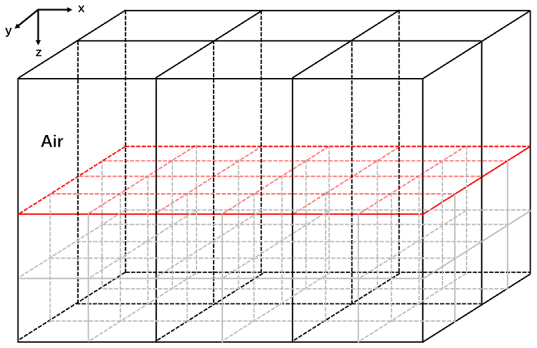Additionally, subgridding technology [33] optimizes the simulation by using CG for the aerial layer and fine grids (FGs) for subsurface media, significantly reducing memory consumption. This strategy is particularly beneficial for AGPR simulations, where the antenna height increases computational demands. In 3D AGPR modeling, the hybrid grid configuration delivers substantial memory-saving advantages, especially with higher antenna elevations.

Despite the potential benefits of combining subgridding techniques with high-order finite-difference time-domain (FDTD) methods, the implementation of such algorithms remains challenging. The primary difficulty lies in managing field coupling at the coarse–fine grid boundary during each time step, which often leads to instabilities, spurious reflections, and accuracy degradation [34]. For example, the Huygens subgridding FDTD method exhibits instability after approximately 1000 time steps [35]. To mitigate these issues, many existing subgridding schemes incorporate additional filtering processes [34,36,37], although these may inadvertently compromise accuracy. Moreover, the larger stencil size of high-order FDTD methods, compared to standard FDTD, increases susceptibility to grid variations, requiring the careful design of coarse- and fine-grid configurations to maintain stability and precision. The additional grid nodes near the coarse–fine boundary further complicate the process, necessitating specialized treatment for high-order differences.

Previous studies have proposed subgridding schemes for two-dimensional problems [38,39,40], using the FDTD(2,4) method—a high-order FDTD variant with second-order temporal and fourth-order spatial accuracy—for the outer coarse-grid (CG) region, while employing standard FDTD for the local fine-grid (FG) region. These hybrid approaches successfully stabilized field communication near the boundary, but they achieved only partial high-order accuracy due to the mixed use of second- and fourth-order methods. This “non-purely” high-order FDTD approach limits grid step sizes to those compatible with second-order differences, preventing full utilization of the larger steps permitted by fourth-order schemes. Consequently, we propose a “purely” subgridding algorithm that fully exploits the advantages of fourth-order differences, enabling larger grid steps and further reducing memory requirements.

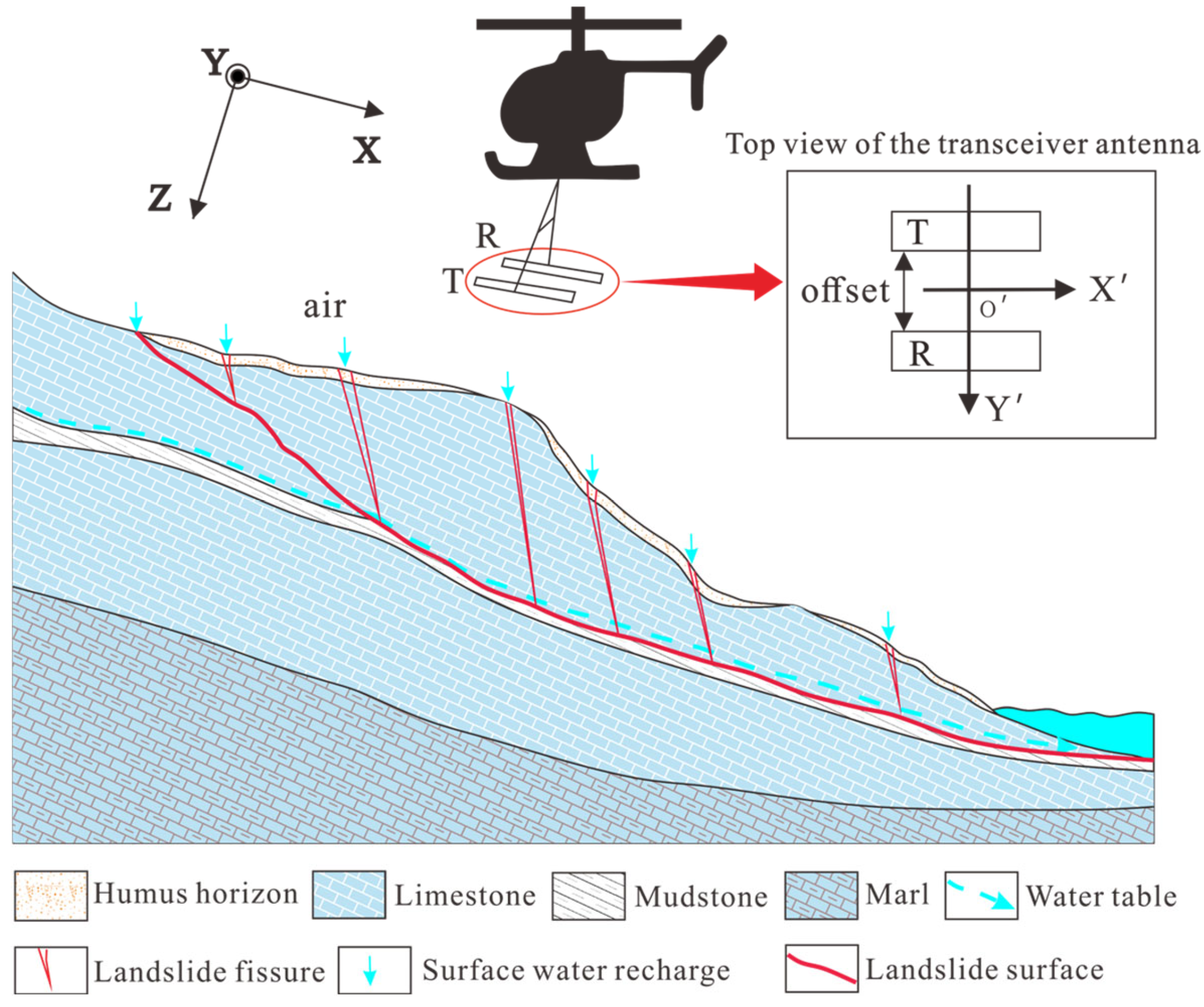
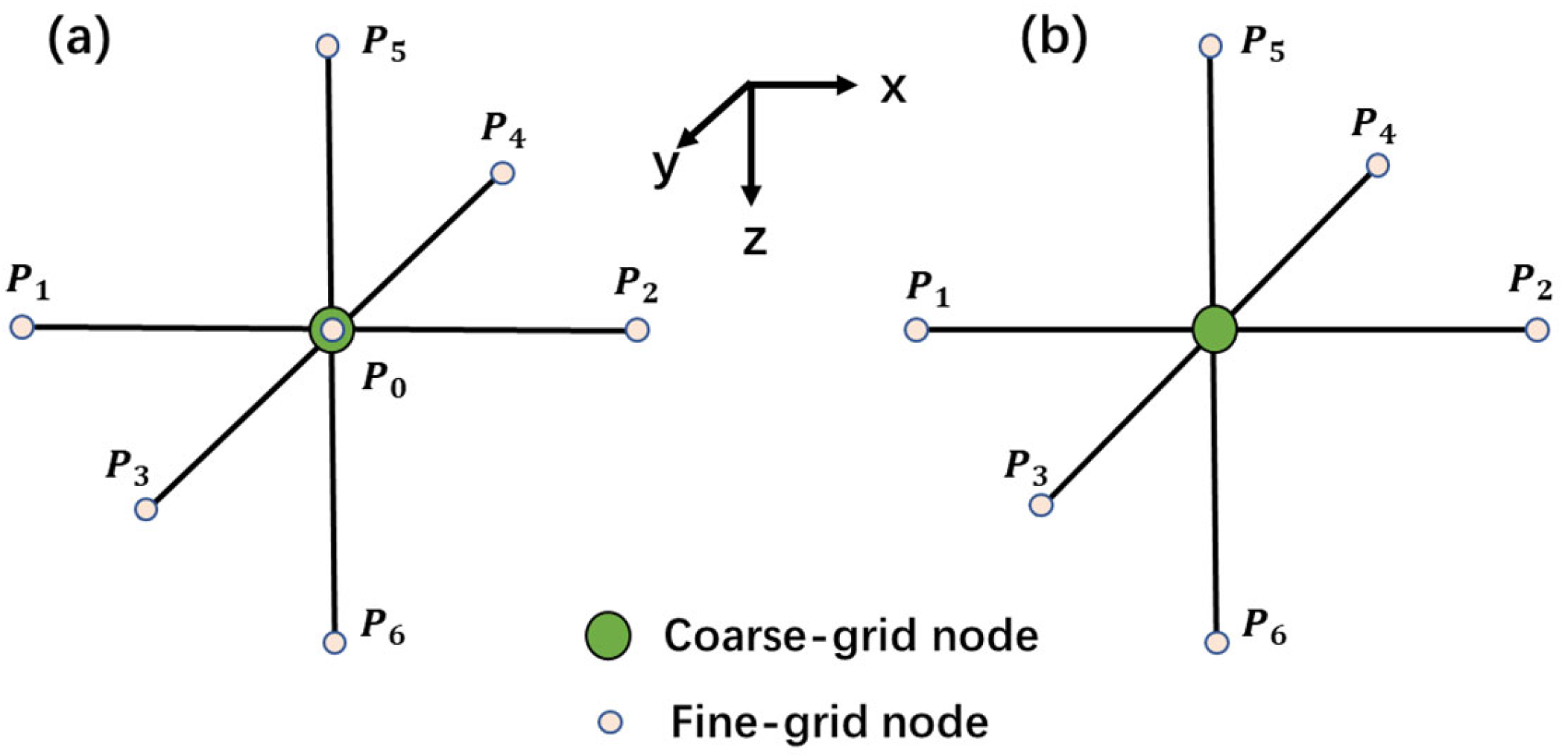
Furthermore, current subgridding techniques are primarily designed for localized anomaly models, where a coarse grid surrounds a locally refined region [33,34,35,36]. These methods are insufficient for simulating complex structures, such as real-world landslides, which feature intricate geological elements like groundwater tables, sliding bodies, and substantial permittivity variations between layers (see Figure 1). Such complexities cannot be effectively modeled using localized target structures. Therefore, developing a novel algorithm capable of accommodating arbitrarily complex structural models holds significant practical value.

To address the aforementioned challenges, this study proposes a novel subgridding scheme that integrates a high-order FDTD(2,4) algorithm for simulating wavefields in 3D models, utilizing carefully designed overlapping grids and virtual grid techniques. This approach represents the first implementation of iterative updates for both coarse- and fine-grid regions using the FDTD(2,4) method, which we term a “purely” high-order FDTD method. To ensure algorithm stability, a weighted correction is applied to the field nodes within the overlapping-grid (OG) region. Compared to traditional FDTD methods, this approach not only improves numerical simulation accuracy through higher-order precision but also enables the use of larger grid step sizes, significantly reducing computational memory requirements. In our implementation, the coarse grid (CG) is allocated to the air layer, while the fine-grid (FG) region is assigned to high-permittivity media. The OG region is strategically positioned in the air layer adjacent to the high-permittivity media to mitigate the effects of long high-order stencils crossing different media interfaces [41]. Furthermore, our algorithm supports arbitrary grid refinement factors (GRFs), optimized based on the maximum permittivity of the medium. These innovations enable the simulation of complex structural models, including landslide scenarios, and facilitate 3D numerical simulations of water-bearing landslide models on conventional computing servers.

The remainder of this article is structured as follows: First, we provide a detailed introduction to the proposed algorithm, focusing on wavefield processing techniques within the OG region under the high-order FDTD(2,4) framework. Second, we perform simulations on various representative models with different GRF values, particularly those involving high-permittivity media such as groundwater. The results are compared with conventional methods in terms of accuracy and memory efficiency. Additionally, the algorithm is validated through a deposition-type landslide model, with an analysis of the response cross-section along a survey line (B-scan). Finally, we assess the algorithm’s stability using extensive numerical simulations, including a counterexample to verify robustness. Simulations of water-bearing media models at varying depths under high-altitude flight conditions, within the memory limits of our server, demonstrate the algorithm’s capabilities. Additionally, we utilize the maximum step size that satisfies the CFL condition and perform extensive iterative calculations to validate the stability of the algorithm for AGPR responses.

2. Method

2.1. Airborne GPR System

Figure 1 schematically demonstrates the operational methodology of airborne ground-penetrating radar (AGPR) for landslide structure detection. The primary objectives of this system are to identify the basement–cover interface and delineate underground aquifers within landslide formations. In the Cartesian coordinate system, the X–Y plane is aligned parallel to the approximate slope surface of the landslide, while the Z-axis is oriented perpendicular to this plane, extending into the subsurface. The landslide surface typically exhibits significant topographic variations. The flight trajectory is maintained parallel to the X-axis, with the transmitting antenna (TA) generating electromagnetic pulses along the x direction. The receiving antenna (RA), dimensionally identical to the TA, maintains a fixed spatial relationship with the transmitter throughout the survey operation. Under idealized stable flight conditions, both TA and RA are maintained at identical altitudes and are symmetrically positioned about the X-axis.

In practical applications, the attitude of the airborne platform can be adjusted to approximate the slope angle. While variations in attitude may significantly influence the observed data, 3D forward modeling enables the calculation of responses at arbitrary orientations by adjusting the antenna position parameters. This methodology ensures theoretical consistency irrespective of platform orientation. Therefore, this study assumes antenna configurations simulate 3D AGPR responses under idealized stable conditions, with constant relative positioning between transmitting and receiving antennas throughout the survey. The antenna plane (denoted as X′-O′-Y′ in Figure 1) is considered parallel to the X–Y plane, with the trajectory of O′ (the geometric center of the TA-RA assembly) defining the survey line.

2.2. 3D FDTD(2,4) Method Integrated with Subgridding Scheme

Maxwell’s equations in a conducting medium, characterized by electric conductivity $\mathsf{\sigma }$ and relative permittivity ${\epsilon }_r$, are solved using second-order temporal and fourth-order spatial approximations, known as the higher-order FDTD(2,4) method [31]. In contrast to the conventional FDTD method, this method utilizes the identical Yee staggered mesh [42] while the spatial difference operator is replaced by a fourth-order accurate stencil. For instance, the quantity $\partial U(i+{\displaystyle \frac{1}{2}},j,k)/\partial x$ can be computed as a fourth-order accurate approximation:

$${\displaystyle \frac{\partial U_{i,j,k}}{\partial x}}={\displaystyle \frac{1}{24∆}}\left(U_{i-1,j,k}-27U_{i,j,k}+27U_{i+1,j,k}-U_{i+2,j,k}\right)$$

(1)

where Δ is the grid size in the corresponding direction. Equation (1) shows that compared with the conventional FDTD(2,2) scheme, the stencil of the FDTD(2,4) scheme has two more nodes. Such differences may lead to variations in the FDTD updating methods and boundary processing techniques of the fields near the interface of coarse and fine grids in subgrid methods, so as to maintain the stability of the numerical calculation and the accuracy of the calculation results. Additionally, where the permittivity of the medium differs greatly, such as the air–ground interface, the accuracy of the calculation of higher-order differences may be greatly affected [41]. Many subgridding schemes encounter stability and material traverse capability [43], which should be handled with more care in higher-order differences. In the 3D grid figure shown in Figure 2, the contrast ratio (the ratio of coarse to fine grid edge lengths, or the grid refinement factor, denoted as Nc, the same hereinafter) is 2. Special treatment is required for the differential calculation of nodes on and near the interface of the coarse and fine grids regions (represented by the red line in Figure 2). For example, one-sided higher-order difference methods are employed to handle the differential calculations at nodes near the boundary [39,40,44]. Different treatment methods result in diverse computational accuracy and stability, occasionally requiring adjustments to the mesh configuration. Even though the computational parameters in both the coarse and fine grid regions of the subgrid method meet the CFL condition, noticeable numerical dispersion and computational instability may still arise. When the long-stencil difference scheme described in Equation (1) is used, crossing media with different physical properties may amplify the dispersion error introduced by the subgrid method, requiring an appropriate algorithm to effectively address this issue.

2.2.1. Subgridding Scheme for a Robust FDTD(2,4) Method

As discussed in the Introduction, conventional subgridding methods with localized grid refinement are insufficient for modeling landslides with complex layered structures (Figure 1). Similarly, multigrid approaches are impractical due to their high computation-al costs, inherent instability, and challenges in handling multi-layer geological formations.

To overcome these limitations, we propose a simplified subgridding scheme, wherein the computational domain is partitioned into an upper coarse-grid (CG) region and a lower fine-grid (FG) region. To partition the two areas, the boundary surface of the physical property (Figure 2), termed the reference plane (RP) in this article, should be determined first, which corresponds to either the air–ground interface (in flat terrain) or a plane passing through the highest topographic point (in undulating terrains).

To ensure numerical stability, the CG and FG regions overlap in a zone spanning the lowest two CG layers in the z direction, as illustrated by the pink dashed line on the x-z cross-section of Figure 3. The center layer of the OG layer is located at the central position in the z direction of the OG grid layer, at a height corresponding to one coarse grid layer above the RP. This grid configuration is beneficial for the accuracy of the higher-order FDTD(2,4) updates under the subgrid. If the grid layout proposed in this study is not employed, the subgrid configuration in the x-z section is illustrated in Figure 3b, where the pink dashed line is located in the middle of the OG region. This is the approach used by most conventional subgridding methods at the interface between the coarse and fine grids. In this case, the fourth-order difference calculation of the fields on the lowest four layers of CGs may cross the physical interface (marked as “Cross” in the following). We will use this grid configuration for comparative calculations to verify the correctness of the algorithm presented in this paper.

This article adopts the complex frequency-shifted Perfectly Matched Layers (PMLs) absorption boundary method [45,46], with the computational domain surrounded by PMLs of the same thickness. Unlike the current subgrid methods that only involve local regions, our PML region is also designed with the same subgrid configuration as the internal non-PML region, and the grid contrast ratio is exactly the same, both equal to $Nc$.

When modeling, it is necessary to select a suitable GRF based on the geoelectric parameters. A suitable $Nc$ in this context specifically refers to the GRF that minimizes memory usage while maintaining calculation accuracy in subgridding FDTD(2,4) calculations. When the excitation signal remains constant, the grid size mostly relies on the dielectric constant of the underground medium (assuming the medium is non-magnetic with a relative magnetic permeability of 1). In the field of ground-penetrating radar applications, the relative permittivity ${\epsilon }_r$ of the ordinary soil ranges from greater than 1 to less than 81, and the relationship between the grid size Δ and ${\epsilon }_r$ is as follows:

$$\mathsf{\Delta }\propto {\displaystyle \frac{1}{\sqrt{{\epsilon }_r}}}$$

(2)

Considering the relative permittivity of air is 1, a suitable grid refinement factor $Nc$ can be given by the following formula:

$$Nc=c\mathrm{e}\mathrm{i}\mathrm{l}\left[\sqrt{{\mathsf{\epsilon }}_{\mathrm{r}\mathrm{m}\mathrm{a}\mathrm{x}}}\right]$$

(3)

where ceil [ ] is a ceiling function and ${\mathsf{\epsilon }}_{\mathrm{r}\mathrm{m}\mathrm{a}\mathrm{x}}$ represents the maximum relative permittivity of the underground medium. For example, when ${\mathsf{\epsilon }}_{\mathrm{r}\mathrm{m}\mathrm{a}\mathrm{x}}$ is 25, a suitable $Nc$ can be chosen as 5, and when ${\mathsf{\epsilon }}_{\mathrm{r}\mathrm{m}\mathrm{a}\mathrm{x}}$ is 40, a suitable $Nc$ can be chosen as 7. In this case, the grid size of the air layer can be maximized, thereby significantly saving computing resources.

2.2.2. Formulation and Time-Marching Scheme

Following the subgrid configuration described above, the FDTD(2,4) scheme was applied to both CG and FG regions. In the OG region, except for the fields at the nodes on the boundaries and sub-boundaries, which are determined using spatial linear interpolation (SLI), the higher-order FDTD computations were used for the other node fields. Utilizing a larger grid size reduces the total number of grids for 3D forward modeling, increases the time step size, and consequently lowers the computational resource requirements. Unlike the hybrid method in [40], which combines the conventional FDTD method for CGs with the higher-order FDTD method for FGs, the proposed approach applies the higher-order FDTD method uniformly across both grid types, achieving more effective memory minimization. To avoid increasing numerical dispersion errors associated with temporal interpolation, this article uses a uniform time step size for iterative calculations in both the coarse and fine grids regions.

Hereinafter, uppercase “$E$” and “$H$” indicate electric and magnetic fields within the CG area, respectively, while lowercase “$e$” and “$h$” denote their counterparts in the FG area. ${\mathsf{\Delta }}_c$ and ${\mathsf{\Delta }}_f$ represent the grid sizes of the coarse and fine grids, respectively. $\mathsf{\Delta }t$ represents the time step, and $n$ represents the $n$th time step of the fields. $\sigma$ and $\epsilon$ represent the conductivity and permittivity of the medium, respectively. Assume the numbers of grid nodes in the CG region along the x, y, and z directions are $N_x,N_y,N_z$, respectively, and those in the FG are $n_x,n_y,n_z$, respectively. For brevity, only the equation for the $E_x$ component is presented [31]:

$$\begin{gathered} E_x^{n+1}\left(i+{\displaystyle \frac{1}{2}},j,k\right) \\ \hspace{1em}\hspace{1em}\hspace{1em}\hspace{1em}\hspace{1em}\hspace{1em}\hspace{1em}\hspace{1em}\hspace{1em}\hspace{1em}\hspace{1em}\hspace{1em}\hspace{1em}=CA{\times E}_x^n\left(i+{\displaystyle \frac{1}{2}},j,k\right) \\ \hspace{1em}\hspace{1em}\hspace{1em}\hspace{1em}\hspace{1em}\hspace{1em}\hspace{1em}-{CB}_z \\ \hspace{1em}\hspace{1em}\hspace{1em}\hspace{1em}\hspace{1em}\hspace{1em}\hspace{1em}\hspace{1em}\hspace{1em}\hspace{1em}\hspace{1em}\hspace{1em}\hspace{1em}\hspace{1em}\hspace{1em}\hspace{1em}\hspace{1em}\hspace{1em}\hspace{1em}\hspace{1em}\hspace{1em}\hspace{1em}\hspace{1em}\hspace{1em}\hspace{1em}\hspace{1em}\times \left[H_y^{n+{\displaystyle \frac{1}{2}}}\left(i+{\displaystyle \frac{1}{2}},j,k-{\displaystyle \frac{3}{2}}\right)-27H_y^{n+{\displaystyle \frac{1}{2}}}\left(i+{\displaystyle \frac{1}{2}},j,k-{\displaystyle \frac{1}{2}}\right) \\ \hspace{1em}\hspace{1em}\hspace{1em}\hspace{1em}\hspace{1em}\hspace{1em}\hspace{1em}\hspace{1em}\hspace{1em}\hspace{1em}\hspace{1em}\hspace{1em}\hspace{1em}\hspace{1em}\hspace{1em}\hspace{1em}\hspace{1em}\hspace{1em}\hspace{1em}\hspace{1em}\hspace{1em}\hspace{1em}\hspace{1em}\hspace{1em}\hspace{1em}\hspace{1em}+27H_y^{n+{\displaystyle \frac{1}{2}}}\left(i+{\displaystyle \frac{1}{2}},j,k+{\displaystyle \frac{1}{2}}\right)-H_y^{n+{\displaystyle \frac{1}{2}}}\left(i+{\displaystyle \frac{1}{2}},j,k+{\displaystyle \frac{3}{2}}\right)\right] \\ \hspace{1em}\hspace{1em}\hspace{1em}\hspace{1em}\hspace{1em}\hspace{1em}\hspace{1em}\hspace{1em}+{CB}_y \\ \hspace{1em}\hspace{1em}\hspace{1em}\hspace{1em}\hspace{1em}\hspace{1em}\hspace{1em}\hspace{1em}\hspace{1em}\hspace{1em}\hspace{1em}\hspace{1em}\hspace{1em}\hspace{1em}\hspace{1em}\hspace{1em}\hspace{1em}\hspace{1em}\hspace{1em}\hspace{1em}\hspace{1em}\hspace{1em}\hspace{1em}\hspace{1em}\hspace{1em}\hspace{1em}\times \left[H_z^{n+{\displaystyle \frac{1}{2}}}\left(i+{\displaystyle \frac{1}{2}},j-{\displaystyle \frac{3}{2}},k\right)-27H_z^{n+{\displaystyle \frac{1}{2}}}\left(i+{\displaystyle \frac{1}{2}},j-{\displaystyle \frac{1}{2}},k\right) \\ \hspace{1em}\hspace{1em}\hspace{1em}\hspace{1em}\hspace{1em}\hspace{1em}\hspace{1em}\hspace{1em}\hspace{1em}\hspace{1em}\hspace{1em}\hspace{1em}\hspace{1em}\hspace{1em}\hspace{1em}\hspace{1em}\hspace{1em}\hspace{1em}\hspace{1em}\hspace{1em}\hspace{1em}\hspace{1em}\hspace{1em}\hspace{1em}\hspace{1em}\hspace{1em}+27H_z^{n+{\displaystyle \frac{1}{2}}}\left(i+{\displaystyle \frac{1}{2}},j+{\displaystyle \frac{1}{2}},k\right)-H_z^{n+{\displaystyle \frac{1}{2}}}\left(i+{\displaystyle \frac{1}{2}},j+{\displaystyle \frac{3}{2}},k\right)\right] \end{gathered}$$

(4)

where $CA$, ${CB}_{\gamma }$ are as follows:

$$CA={\displaystyle \frac{2\epsilon -\sigma \mathsf{\Delta }t}{2\epsilon +\sigma \mathsf{\Delta }t}}, {CB}_{\gamma }={\displaystyle \frac{\mathsf{\Delta }t}{12{\mathsf{\Delta }}_c\left(2\epsilon +\sigma \mathsf{\Delta }t\right)}}, \gamma =y,z.$$

(5)

The iterative formula for updating the $e_x$ field at the FG nodes is similar. The $E_x$ field at grid nodes, with the exception of those located on the bottom two layers of the CG (the layer $N_z$ − 2 and layer $N_z$ − 1, as shown in Figure 4a) and the top two layers of the FG (as shown in Figure 4b), can be updated using Equation (4). However, the update of the $E_x$ at layer $N_z$ − 2 is different. It involves not only the two $H_y$-nodes above the $E_x$-node ($H_y^2$- and $H_y^3$-nodes in Figure 4a) and one $H_y$-node below it ($H_y^1$-nodes in Figure 4a), but also the VN field $H_{yv}$, located beneath the OG region (represented by the unfilled circle in Figure 4a). The updated formula is as follows:

$$\begin{gathered} E_x^{n+1}(i+{\displaystyle \frac{1}{2}},j,N_z-2) \\ \hspace{1em}\hspace{1em}\hspace{1em}\hspace{1em}\hspace{1em}\hspace{1em}\hspace{1em}\hspace{1em}\hspace{1em}\hspace{1em}\hspace{1em}\hspace{1em}\hspace{1em}\hspace{1em}\hspace{1em}\hspace{1em}\hspace{1em}\hspace{1em}\hspace{1em}\hspace{1em}\hspace{1em}\hspace{1em}\hspace{1em}\hspace{1em}\hspace{1em}\hspace{1em}=CA\times E_x^n(i+{\displaystyle \frac{1}{2}},j,N_z-2)-C{B}_z[H_y^{n+{\displaystyle \frac{1}{2}}}(i+{\displaystyle \frac{1}{2}},j,N_z-{\displaystyle \frac{7}{2}}) \\ \hspace{1em}\hspace{1em}\hspace{1em}\hspace{1em}\hspace{1em}\hspace{1em}\hspace{1em}\hspace{1em}\hspace{1em}\hspace{1em}\hspace{1em}\hspace{1em}\hspace{1em}\hspace{1em}\hspace{1em}\hspace{1em}\hspace{1em}\hspace{1em}\hspace{1em}\hspace{1em}\hspace{1em}\hspace{1em}\hspace{1em}\hspace{1em}\hspace{1em}-27H_y^{n+{\displaystyle \frac{1}{2}}}(i+{\displaystyle \frac{1}{2}},j,N_z-{\displaystyle \frac{5}{2}})+27H_y^{n+{\displaystyle \frac{1}{2}}}(i+{\displaystyle \frac{1}{2}},j,N_z-{\displaystyle \frac{3}{2}}) \\ \hspace{1em}\hspace{1em}\hspace{1em}\hspace{1em}\hspace{1em}\hspace{1em}\hspace{1em}\hspace{1em}\hspace{1em}\hspace{1em}\hspace{1em}\hspace{1em}\hspace{1em}\hspace{1em}\hspace{1em}\hspace{1em}\hspace{1em}\hspace{1em}\hspace{1em}\hspace{1em}\hspace{1em}\hspace{1em}\hspace{1em}-H_{yv}^{n+{\displaystyle \frac{1}{2}}}(i+{\displaystyle \frac{1}{2}},j)]+C{B}_y[H_z^{n+{\displaystyle \frac{1}{2}}}(i+{\displaystyle \frac{1}{2}},j-{\displaystyle \frac{3}{2}},N_z-2 \\ \hspace{1em}\hspace{1em}\hspace{1em}\hspace{1em}\hspace{1em}\hspace{1em}\hspace{1em}\hspace{1em}\hspace{1em}\hspace{1em}\hspace{1em}\hspace{1em}\hspace{1em}\hspace{1em}\hspace{1em}\hspace{1em}\hspace{1em}\hspace{1em}\hspace{1em}\hspace{1em}\hspace{1em}\hspace{1em}\hspace{1em}\hspace{1em}\hspace{1em}-27H_z^{n+{\displaystyle \frac{1}{2}}}(i+{\displaystyle \frac{1}{2}},j-{\displaystyle \frac{1}{2}},N_z-2)+27H_z^{n+{\displaystyle \frac{1}{2}}}(i+{\displaystyle \frac{1}{2}},j+{\displaystyle \frac{1}{2}},N_z \\ \hspace{1em}\hspace{1em}\hspace{1em}\hspace{1em}\hspace{1em}\hspace{1em}\hspace{1em}\hspace{1em}\hspace{1em}\hspace{1em}\hspace{1em}\hspace{1em}\hspace{1em}\hspace{1em}\hspace{1em}\hspace{1em}-2)-H_z^{n+{\displaystyle \frac{1}{2}}}(i+{\displaystyle \frac{1}{2}},j+{\displaystyle \frac{3}{2}},N_z-2)] \end{gathered}$$

(6)

where, $H_{yv}^{n+{\displaystyle \frac{1}{2}}}\left(i+{\displaystyle \frac{1}{2}},j\right)$ represents the magnetic field component $H_{yv}$ at the VN, located half a depth ${\mathsf{\Delta }}_c$ below the OG area. It is derived through SLI from the magnetic fields $h_y$ in the FG area.

Similarly, the update of the $e_x$ field on the second layer (marked as “1” in Figure 4b) within the OG region, as indicated by the blue arrows, requires the magnetic field $h_{yv}$ at the VN, located half a ${\mathsf{\Delta }}_f$ above the OG area. During each iteration, the $h_{yv}$ field is updated via SLI from the magnetic fields $H_y$ at the corresponding spatial interpolation nodes in the CG region. The $E_x$ fields at the bottom boundary of the CG (marked as “$N_z$ − 1” in Figure 4a) are directly obtained through SLI from the $e_x$ fields at the corresponding nodes in the FG region. Similarly, the $e_x$ fields on the top boundary of the FG region (marked as “0” in Figure 4b) are derived by SLI from the $E_x$ fields at the corresponding nodes in the CG region.

2.2.3. Spatial Linear Interpolation and Weighted Correction

As mentioned earlier, the fields at VNs and at the boundaries between coarse and fine grids need to be obtained through SLI. The interpolating fields at these boundaries are a critical aspect of the subgridding FDTD method [32]. The SLI method we employ is applicable to subgrids with any contrast ratio. Figure 5 illustrates the interpolation process for the electric field component from the CG to the FG region. The 8 $E_x$-nodes (highlighted in red in Figure 5) surrounding the target $e_x$-node (indicated by the green arrow) are determined first, and the $e_x$ field is then interpolated using the following equation:

$$e_x={\displaystyle \frac{1}{V}}\sum _{k=1}^8{c}_k{E}_x^k$$

(7)

where $V$ represents the volume of the cuboid defined by the 8 $E_x$-nodes, and $c_k$ denotes the volume of the sub-cuboid whose diagonal is the line from the $e_x$-node to the $E_x^{8-k}$-$\mathrm{n}\mathrm{o}\mathrm{d}\mathrm{e}$. The interpolation method is essentially a 3D linear interpolation method based on volume weighting, making is effective for any GRF.

When performing linear interpolation from the FG to the CG, a CG node may coincide with an FG node. In such cases, the parity of Nc must be considered. As illustrated in Figure 6, there can be either 7 (see Figure 6a) or 6 (see Figure 6b) closely adjacent FG nodes surrounding a CG node located at $P_0$. Taking the $E_x$-node of the CG as an example, its interpolation formula is as follows:

$$E_x=\left\{\begin{array}{ll}{ e}_x\left(P_0\right)& if Nc is odd \\ {\displaystyle \frac{1}{6}}{\displaystyle \sum _{k=1}^6}{e}_x\left(P_k\right)& if Nc is even\end{array}\right.$$

(8)

where $P_k$ (k = 1, 2, …, 6) represents the six FG nodes surrounding the node $P_0$.

Using SLI to interpolate the fields at the boundaries between coarse and fine grids alone may not fully ensure the stability of the subgridding FDTD method. Therefore, it is still necessary to ensure a smooth transition between the coarse and fine grids. The fields at the coarse and fine grid nodes within the OG region are calculated using the FDTD(2,4) method. Once the fields at all nodes in the OG region are fully calculated, a weighted correction is performed based on their depth in the z direction within the OG region. As illustrated in Figure 4, there is only one $E_x$-node in the OG region, located at the center of the OG region in z direction. Accordingly, the correction formula for $E_x$ in the OG region is as follows:

$$E_x=\left(E_x+{\overline{e}}_x\right)/2$$

(9)

where ${\overline{e}}_x$ represents the corresponding field $e_x$ at the $E_x$-node, which can be obtained using Equation (8). Similarly, as shown in Figure 4, there are 2Nc − 2 $e_x$-nodes inside the OG region, and their correction formula is as follows:

$$e_x\left(k\right)=\left[k{e}_x\left(k\right)+(2N_c-k){\overline{E}}_x\left(k\right)\right]/\left(2Nc\right)$$

(10)

where $k$ (=1, 2, …, 2Nc − 2) represents the z directional index of the $e_x$-node within the OG region. ${\overline{E}}_x\left(k\right)$ denotes the field value at the $e_x\left(k\right)$-node, obtained through SLI using Equation (7).

2.2.4. Update Procedure of the Subgridding FDTD(2,4) Method

In this part, a summary of the update procedure for our subgridded FDTD(2,4) method is shown. It is assumed that the field update has been advanced to time step $n$, and that all the electric and magnetic fields in the CG area, FG area, and at VNs are known. Then, the update process is made up of the following sequence of computing steps:

• Update fields $E$ in the CG area except those on the lower boundary based on fields $H$ inside the CG area and fields $H_{\gamma v}$ $\left(\gamma =x,y\right)$ at the VNs, and then update fields $e$ on the upper boundary based on the fields $E$ calculated in this step using the method shown in Equation (7).
• Update fields $e$ in the FG area except those on the upper boundary based on fields $h$ inside the FG area and fields $h_{\gamma v}$ $\left(\gamma =x,y\right)$ at the VNs, and then update fields $E$ on the lower boundary based on the fields $e$ calculated in this step using the method shown in Equation (8).
• Correct the fields $E$ in the OG area according to the method shown in Equation (9).
• Correct the fields $e$ in the OG area according to the method shown in Equation (10).
• Calculation fields $E_{\gamma v}$ and $e_{\gamma v}$ $\left(\gamma =x,y\right)$ at VN using the SLI method shown in Equations (8) and (7), respectively.
• Update fields $h$ in the FG based on the fields e and $e_{\gamma v}\left(\gamma =x,y\right)$, and then calculate fields $H_{\gamma v}$ $\left(\gamma =x,y\right)$ using the SLI method shown in Equation (8).
• Update fields $H$ in the CG based on the fields $E$ and $E_{\gamma v}\left(\gamma =x,y\right)$, and then calculate fields $h_{\gamma v}$ $\left(\gamma =x,y\right)$ using the SLI method shown in Equation (7).
• Advance simulation time step: $n$ = $n$ + 1, and recycle.

3. Numerical Experiments

Using the algorithm described in the previous section, we developed a 3D forward modeling program in C++ (version 20). To ensure a consistent comparison of memory consumption across different models, the same thickness of Perfectly Matched Layers (PML) was applied for all methods. The computations were conducted on a server with 576 GB of memory, capable of supporting up to 56 parallel threads. Only models with memory requirements within the server’s capacity were eligible for simulation.

Landslide models are often characterized by water-rich media with relatively high permittivity. Under the constraints of the CFL condition, traditional FDTD methods require the entire computational domain to be discretized with smaller grid sizes and shorter time steps to accommodate the high permittivity medium. This approach imposes a significant demand on computational resources. The larger the permittivity of the underground medium, the higher the computational cost. In contrast, the subgridding method proposed in this article employs CGs for the air layer and FGs for the underground region. This design reduces the number of grids in the air layer, thereby significantly decreasing computational resource consumption. Consequently, this method allows for the simulation of larger computational domains or landslide models with higher permittivity media. Moreover, the advantages of this method become increasingly evident as the flight altitude increases.

In the following numerical simulation examples, models with relatively low permittivity are used to verify the correctness of the algorithm. The memory consumption for these calculations is within the capacity of our server, ensuring that standard FDTD or standard FDTD(2,4) methods can simulate these models. This allows for a comparison between the simulation results of our proposed method and those of the standard FDTD methods. In contrast, landslide models containing media with higher permittivity (such as water-rich soil) can only be computed using our proposed method, as the memory consumption of standard methods far exceeds the capacity of our server.

3.1. Two-Layer Model

We begin by performing numerical tests on a simple two-layer model to validate the accuracy of the algorithm. The overlying rock layer has a thickness of 3.6 m, with a relative permittivity and a conductivity of 9 and 2 mS/m. The underlying bedrock has a relative permittivity of 4 and a conductivity of 1 mS/m. The radar antenna is positioned 3.6 m above the ground, with the TA measuring 0.72 m × 0.36 m × 0.18 m and an offset of 1.44 m between the TA and the RA. The TA excites a current signal in the x direction with a center frequency of 96.6 MHz.

$$I(t)=\left\{\begin{array}{c}{\sum }_{k=0}^3{h}_k\cos \left({\displaystyle \frac{2n\pi t}{T}}\right)\hspace{1em}\hspace{1em}0<t<T \hfill \\ \hspace{1em}0\hspace{1em}\hspace{1em}\hspace{1em}\hspace{1em}\hspace{1em} other\end{array}\right.$$

(11)

where the current signal is the first derivative of the Blackman–Harris window function [47,48], with T set to 1.14/fc, where fc is the center frequency. The coefficients $h_k(k=0,1,2,3)$ are taken as 0.35322222, −0.488, 0.145, and −0.010222222, respectively. The calculation results of the method proposed in this article are compared with those of the standard FDTD method and the FDTD(2,4) method.

The PMLs in all methods have the same thickness, equivalent to 15 times the coarse grid cell size. Other calculated parameters are listed in

Table 1. The computational parameters for the 3D forward modeling of the two-layer model.

Method		Grid Size (cm)	Number of Nodes	Time Step (ns)
standard FDTD		3	1081 × 1057 × 925	0.05775
FDTD(2,4)		6	541 × 529 × 463	0.099
subFDTD(2,4) − Nc = 3	CG	18	181 × 177 × 108	0.099
	FG	6	541 × 529 × 148

, with all parameters meeting the CFL condition. The standard FDTD method requires small grids throughout the entire computation domain, achieving high spatial and temporal resolutions. However, this approach is memory-intensive, time-consuming, and susceptible to cumulative errors over extended simulation durations.

The FDTD(2,4) method doubles the grid size, resulting in a decrease in the number of grids in the computational domain and thereby saving a considerable number of computational resources. The subgridding scheme proposed in this article (labeled as “subFDTD(2,4) − $Nc$ = m”, where m represents the value of the GRF) further reduces the number of grids in the air layer, consequently decreasing computation time as well.

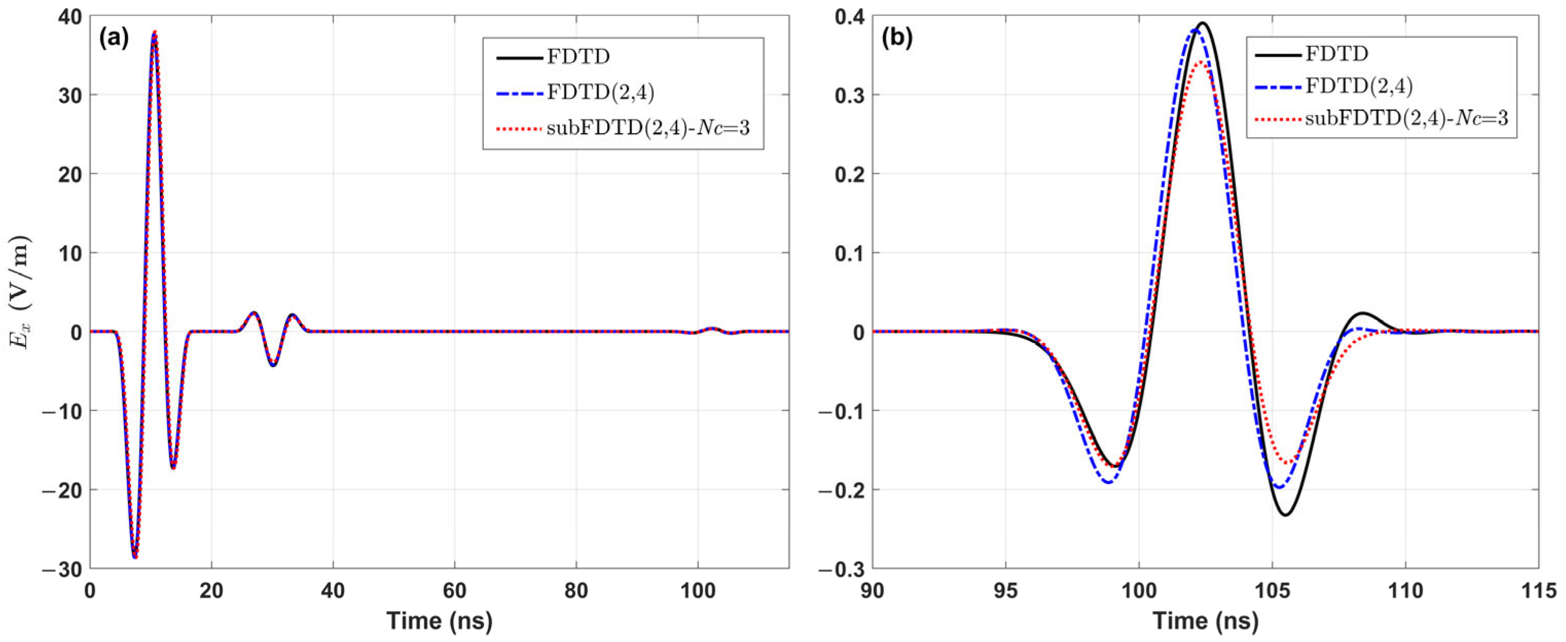
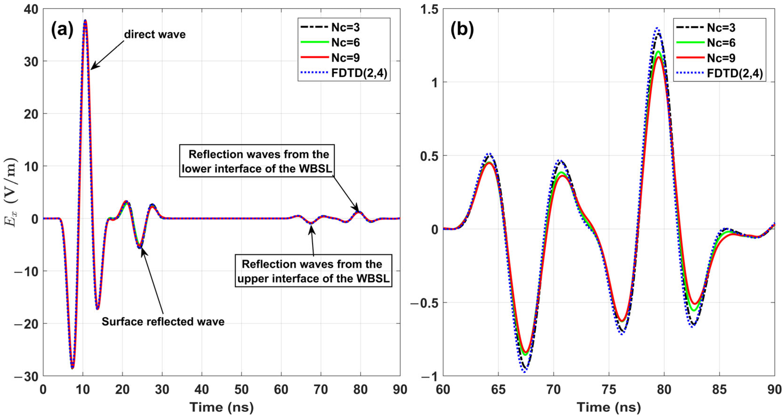
Figure 7 presents the response curves calculated using the three methods outlined in Table 1, demonstrating consistent results across all approaches. The direct wave is observed before 18 ns, the surface reflection wave occurs from 22 to 38 ns, and the bedrock reflection wave is detected from 93 to 110 ns. Notably, the response curves generated by the higher-order difference method exhibit a smoother profile.

Both our method and the standard FDTD(2,4) method use the same difference scheme and share the same spatial steps size in FG regions, resulting in relatively small differences between the response curves produced by these two methods. However, since our method uses a larger grid size in the CG region and incorporates operations such as SLI (see Equation (7)) and weighted corrections (see Equation (10)) in the OG region, these factors contribute to a smoother reflection wave curve compared to the standard FDTD(2,4) method.

This is clearly illustrated in Figure 7. The standard FDTD method, which uses the smallest grid size and correspondingly a smaller time step size, is less influenced by the smoothing factors mentioned earlier, leading to more noticeable waveform variations. Slight time deviations among the waveforms are observed due to differences in stencil lengths and discretization grid sizes.

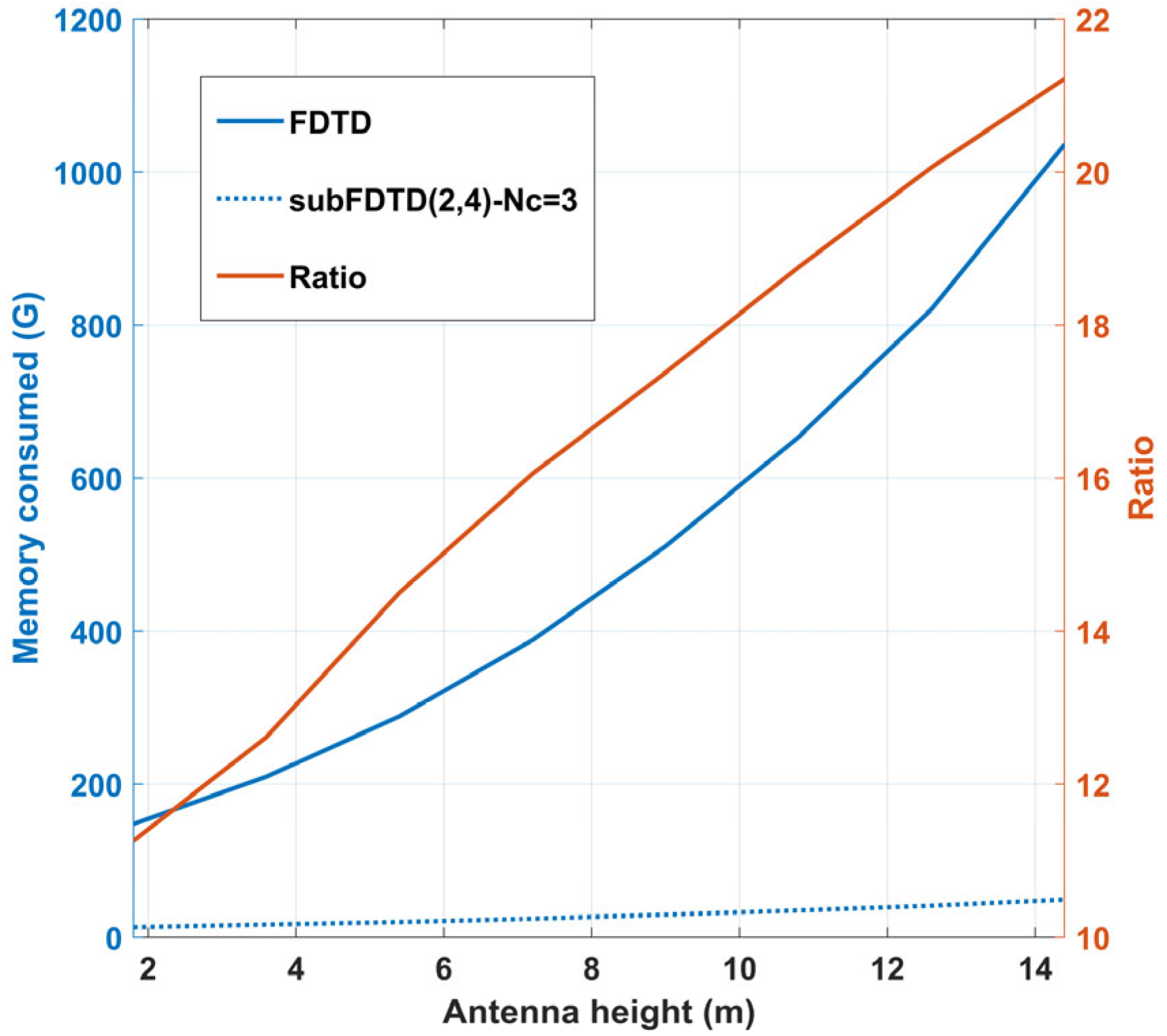
Figure 8 shows the total memory consumption for the 3D forward modeling at varying antenna heights. As shown, the memory consumption of the standard FDTD method increases more rapidly with the rise in antenna height. Additionally, Figure 8 provides a ratio curve comparing the computational memory consumption between the standard FDTD method and our method, demonstrating that the memory consumption of the standard FDTD method is approximately 11 to 22 times greater than that of our method.

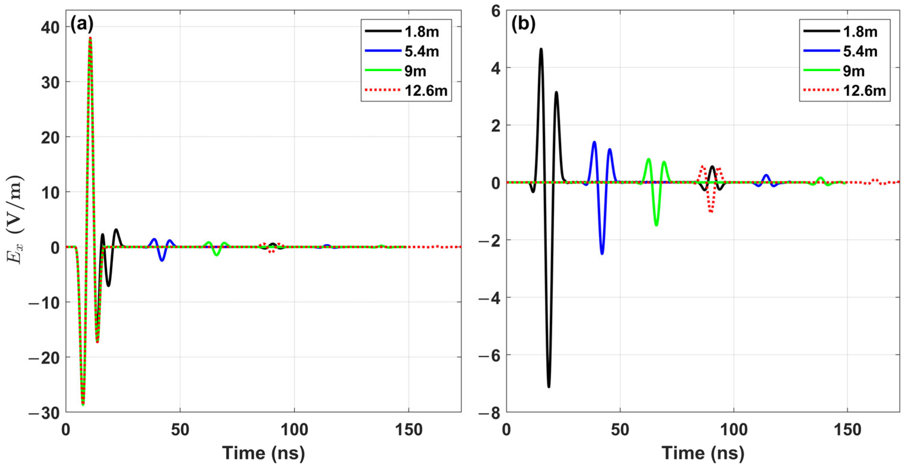
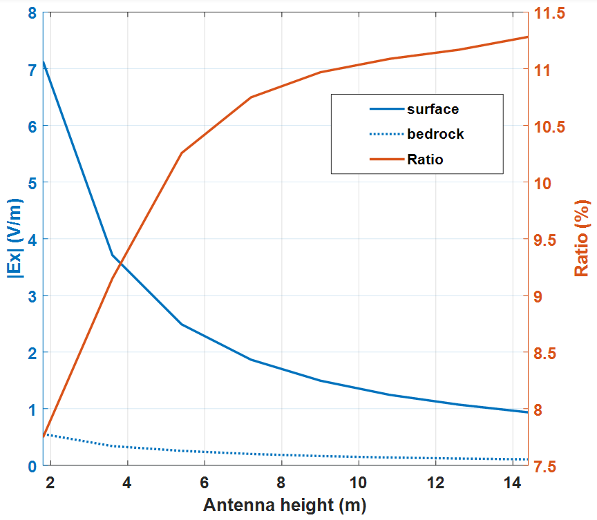
Figure 9 displays the response curves at various antenna heights, each containing the corresponding direct wave, surface reflection wave, and bedrock reflection wave. Due to the fixed positions of the transmitting and receiving antennas, the direct wave portion of each curve remains virtually identical. As the antenna height increases, the arrival times of the reflection waves from the surface and bedrock are sequentially delayed. As the antenna height increases, the waveforms of the various reflection waves remain similar, but their maximum amplitudes gradually decrease. The ratio of the maximum amplitude of the bedrock reflection wave to that of the surface reflection wave increases with height (see Figure 10). At a certain flight altitude, a larger ratio implies that in the total energy of the reflected wave from the earth surface and the bedrock surface, the energy allocated to the bedrock surface is relatively greater, enhancing the identification of the bedrock surface. As the flight altitude increases, the maximum amplitudes of both reflected waves decrease. However, the ratio of their maximum amplitudes increases, implying that while the energy of the reflection wave acting on the bedrock interface decreases, its proportion relative to the energy of the surface reflection wave grows. If the bedrock reflection signal has a sufficiently high signal-to-noise ratio, a larger ratio becomes practically significant for identifying the underground bedrock surface. Conversely, regardless of how large the ratio is, it holds no practical significance if the signal-to-noise ratio of the bedrock reflection signal is insufficient. That is particularly interesting in areas with complex surface conditions such as rugged terrain or dense vegetation, where raising the GPR to an appropriate height may actually enhance its ability to detect deeper geological structures. A practical example of this is provided in [3].

To validate the accuracy of the proposed algorithm in simulating water-containing models, the upper layer of the two-layer model was replaced with water, referred to as the “surface water two-layer model”. The water lay had a conductivity of 50 mS/m, a relative permittivity of 81, and a thickness of 0.9 m. The lower layer has a conductivity of 5 mS/m and a relative permittivity of 9. The antenna height was set at 2.7 m, while other computational parameters remain unchanged from the two-layer model mentioned above. For the standard FDTD method, the grid size was set to 1 cm, while for the standard FDTD(2,4) method, it was set to 2 cm. In the proposed subgridding method, an appropriate refinement factor of $Nc$ = 9 was selected based on Equation (3), resulting in coarse and fine grid sizes of 18 cm and 2 cm, respectively. The memory consumption for these three methods were 3144.3 GB, 393.3 GB, and 111.5 GB, respectively. Due to insufficient server memory, the standard FDTD method could not be executed, so only the results from the standard FDTD(2,4) method were available for comparison (see Figure 11). It can be observed that, before 19 ns, the direct waves obtained by both methods are almost identical, except for a slight time delay. Between 19 ns and 31 ns, corresponding to reflections from the water surface, the waveforms show good agreement. However, the waveforms generated by the standard FDTD(2,4) method exhibit a slight time delay relative to those from the subgridding method. For the late reflection wave from the bedrock interface, the waveforms from both methods are generally consistent, but the smoothing effect in the subgridding method results in a slightly lower peak amplitude compared to the standard FDTD method. As noted earlier, this smoothing effect arises from operations such as 3D spatial interpolation and weighted correction within the subgrid algorithm.

These results demonstrate that our method enables the computation of AGPR responses for water-containing models on ordinary servers, overcoming the limitations of standard methods. Both examples demonstrate that despite utilizing the largest possible grid size within the constraints of the CFL condition, the results produced by our subgridding method are in excellent agreement with those obtained from the standard FDTD and FDTD(2,4) methods.

3.2. Three-Layer Model with a High-Permittivity Layer

The three-layer model was created by incorporating a water-bearing soil layer (WBSL) as an intermediate layer into the original two-layer model described above. The WBSL layer has a relative permittivity of 25, a conductivity of 5 mS/m, and a thickness of 36 cm. The thickness of the first layer was adjusted to 2.16 m, and the antenna height was set to 2.7 m. Other model parameters remained the same as those in the original two-layer model. This three-layer model is referred to as the WBSL model. The responses calculated for $Nc$ values of 3, 6, and 9 are compared with the results obtained using the standard FDTD method.

Table 2. Some forward modeling parameters used for the WBSL model.

Methods		Grid Size (cm)	Number of Grid Nodes (Including PMLs)	Time Step Size (ns)	Number of Time Step	Total Memory (G)
standard FDTD		1.8	1421 × 1401 × 1196	0.03466	2597	479.57
FDTD(2,4)		3	865 × 853 × 730	0.0495	1819	116.20
$\mathrm{subFDTD}(2,4)-Nc$ = 3	9	9	309 × 305 × 180	0.0495	1819	50.24
	3	3	865 × 853 × 229
$\mathrm{subFDTD}(2,4)-Nc$ = 5	18	18	169 × 167 × 132	0.0594	1516	39.14
	3.6	3.6	721 × 711 × 201
$\mathrm{subFDTD}(2,4)-Nc$ = 6	18	18	169 × 167 × 98	0.0495	1819	67.17
	3	3	859 × 847 × 238
$\mathrm{subFDTD}(2,4)-Nc$ = 9	18	18	169 × 167 × 98	0.033	2728	225.08
	2	2	1273 × 1255 × 331
$\mathrm{subFDTD}(2,4)-Nc$ = 9	18	18	185 × 183 × 107	0.033	3031	275.60
	2	2	1417 × 1399 × 349

shows some of the calculation parameters, while others remain unchanged from the above example of the original two-layer model.

From Table 2, it is evident that the standard FDTD method requires a significant amount of memory. In contrast, the subgridding FDTD(2,4) method proposed in this article significantly reduces memory consumption. As Nc increases, memory consumption gradually rises, with the minimum consumption occurring at Nc = 5. Since the maximum relative permittivity of the WBSL model is 25, the optimal GRF, according to Equation (3), is exactly 5. At this point, a relatively large grid size can be used, allowing for a larger time step, which minimizes memory usage. As a result, the memory usage is reduced by 66.32% and 91.84% compared to the standard FDTD(2,4) method and the standard FDTD method, respectively.

However, setting too large a GRF will increase the number of FGs, resulting in higher memory consumption. According to Equation (3), when the maximum relative permittivity of the model is greater than 64 and less than or equal to 81, an appropriate Nc is 9. A typical example is a landslide model containing groundwater. Employing the standard FDTD method to simulate such a 3D model on an ordinary server often leads to insufficient memory capacity.

Figure 12 illustrates the response curves of the WBSL model computed using four different methods, respectively. The direct wave, surface reflection waves, and reflection waves from the upper and lower boundaries of the WBSL are distinctly identifiable. The reflection waves from the upper and lower boundaries of the WBSL model can be observed at approximately 67.43 ns and 79.48 ns. The time interval between the two peaks of the reflection waves matches the theoretical calculation value of the round-trip travel time: ${\displaystyle \frac{2\times 0.36}{c/\sqrt{25}}}=12 \mathrm{n}\mathrm{s}$ (where $c$ is the speed of light). All the curves effectively interpret the underground WBSL, and there is little difference between these reflected waveforms.

3.3. Landslide Models

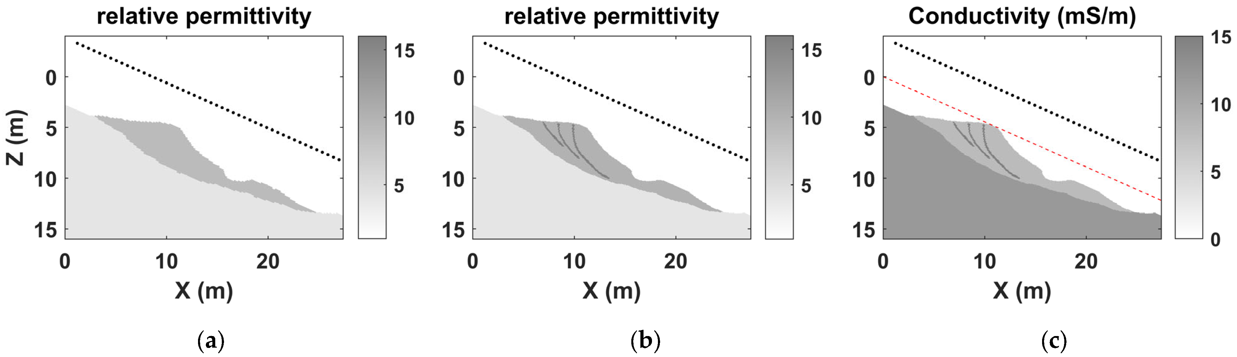
The accumulation-type landslide model depicted in Figure 13a comprises a surface soil layer and bedrock featuring an arcuate slip surface. The slope has an inclination angle of approximately 24°, with the soft surface soil layer reaching a maximum thickness of about 4 m. The landslide’s slope exhibits an undulating profile, characterized by a convex segment spanning from 10 m to 11 m and a concave segment extending from 15.5 m to 18.5 m. The surface stratum, constituted by precarious soil formations, is susceptible to fracturing when subjected to external influences, which may culminate in the occurrence of landslide calamities. Figure 13b,c illustrates the soil stratum models with three developing fissures. The AGPR traversed a linear path parallel to the slope’s surface, maintaining an altitude of 3 m above the red dashed line indicated in Figure 13c. At each measurement site, the excitation current of the AGPR is aligned with the survey line trajectory, ensuring directional consistency, while the center frequency fc of the excitation signal (see Equation (11)) is 80 MHz.

Numerical simulations were performed using the subgridding approach proposed in this article, with a GRF of 3. The coarse and fine grid sizes were 15 cm and 5 cm, respectively, and the time step was set to 0.0825 ns. Figure 14 and Figure 15 present the simulation results of the two models shown in Figure 13.

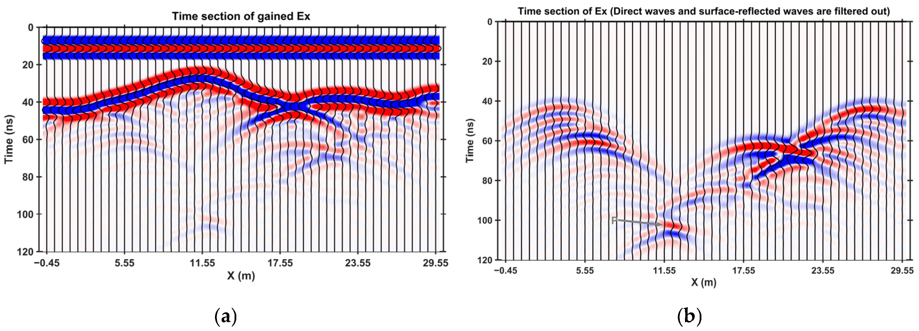
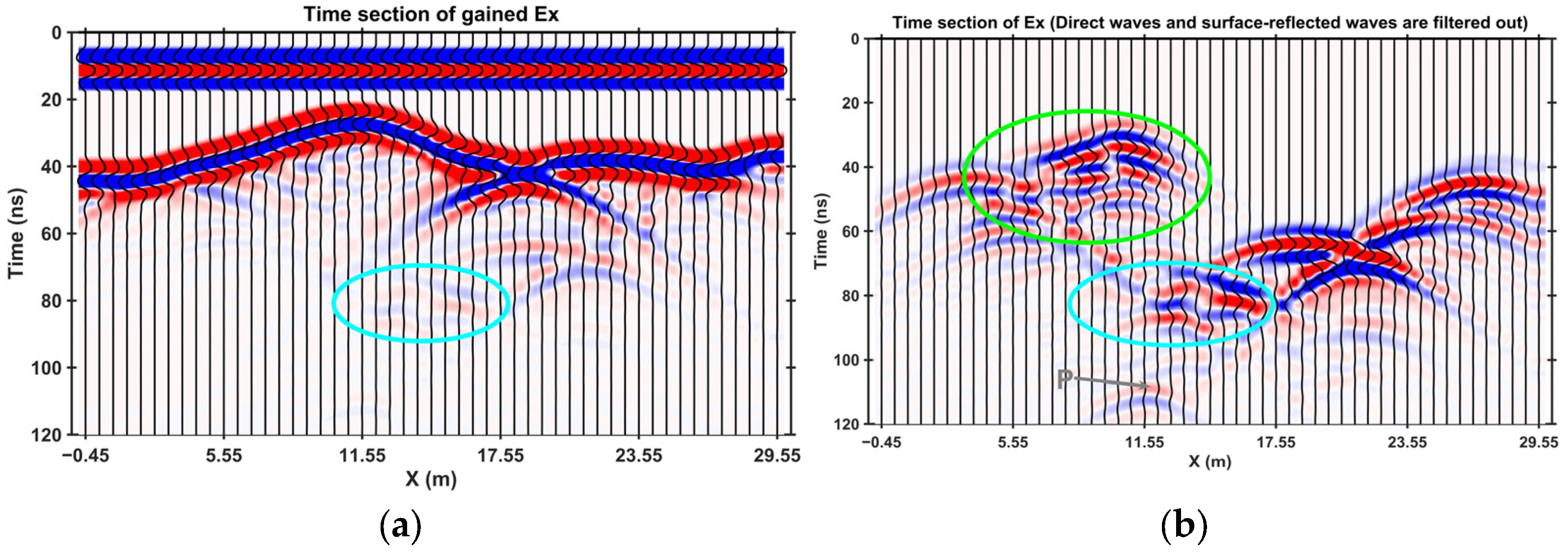
Figure 14a illustrates the time-section diagram for the initial landslide model (Figure 13a). The direct wave, prominently visible prior to 20 ns, is clearly discernible. Below this direct wave, the event of the surface reflection wave displays lateral undulations that mirror the surface topography of the landslide. A multitude of events, inclined both to the left and right, are evident beneath the surface reflection wave. They are indicative of the lateral discontinuities on the ground surface, particularly at the concave segment of the surface soil. Further below, several arcuate hyperbolic events appear, signifying the reflection signals originating from the bedrock surface of the landslide. The vertices of these hyperbolas bear a direct correlation to the morphological features of the bedrock surface. Figure 15b provides a refined view of the time-section diagram, achieved by eliminating the direct wave and the surface reflection wave from Figure 14a. This refinement renders the reflection wave events of the bedrock surface more conspicuous, thereby enhancing the clarity of the lateral distribution of the subsurface bedrock surface. The development of fissures within a landslide induces modifications on the time-section profiles. Upon comparing Figure 14 with Figure 15, it becomes evident that the area delineated by the cyan ellipse in Figure 15 significantly deviates from its counterpart in Figure 14. Following the removal of the direct wave and the surface reflection wave, the region bounded by the green ellipse in Figure 15b also demonstrates notable disparities when contrasted with the corresponding area in Figure 14b. Therefore, by analyzing the variations in the time-section profiles across different observational stages, one can acquire a deeper understanding of the internal structural transformations of the landslide. This implies that the progression of fissure development within a landslide can be detected and monitored through the use of AGPR.

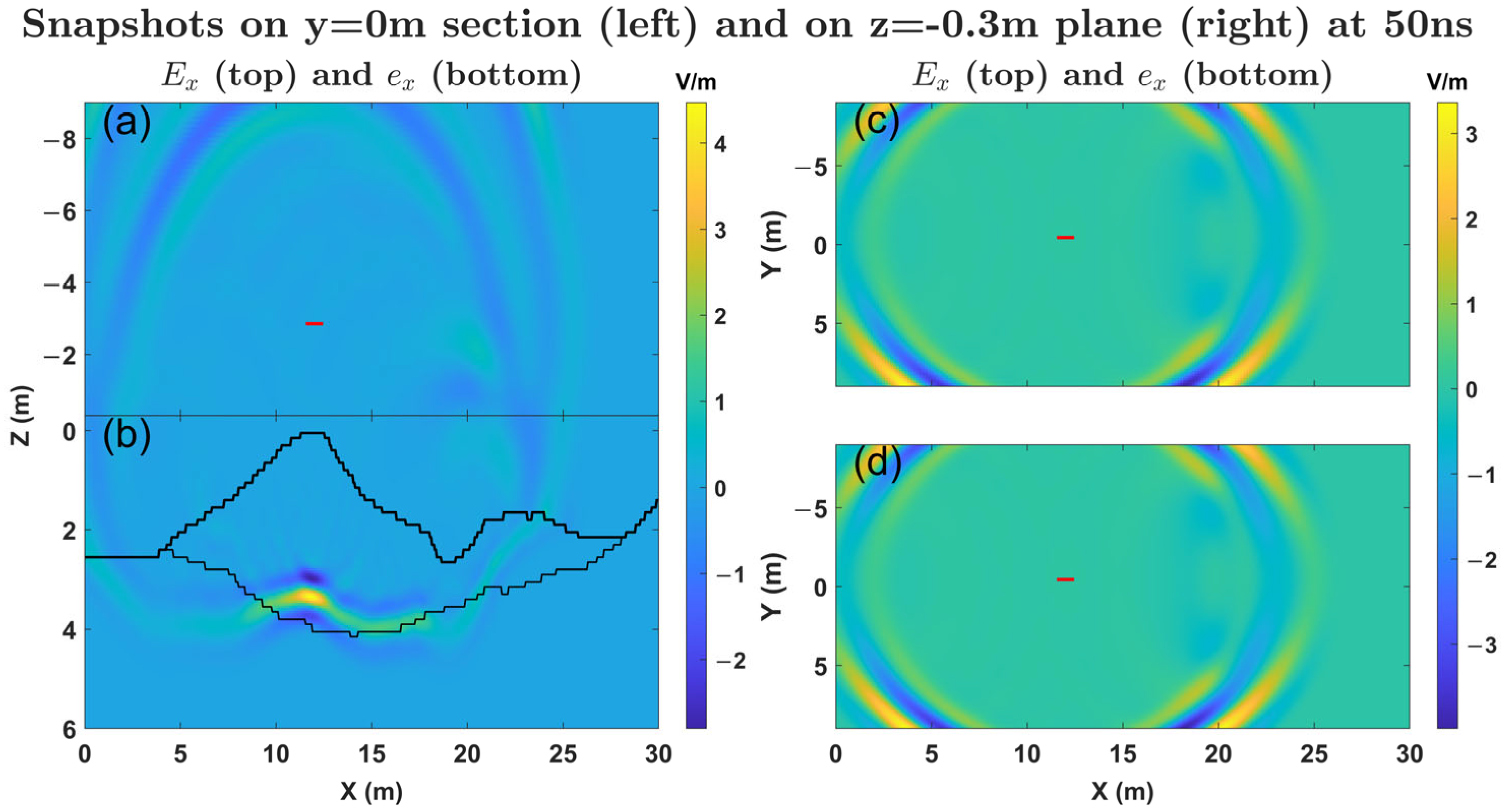
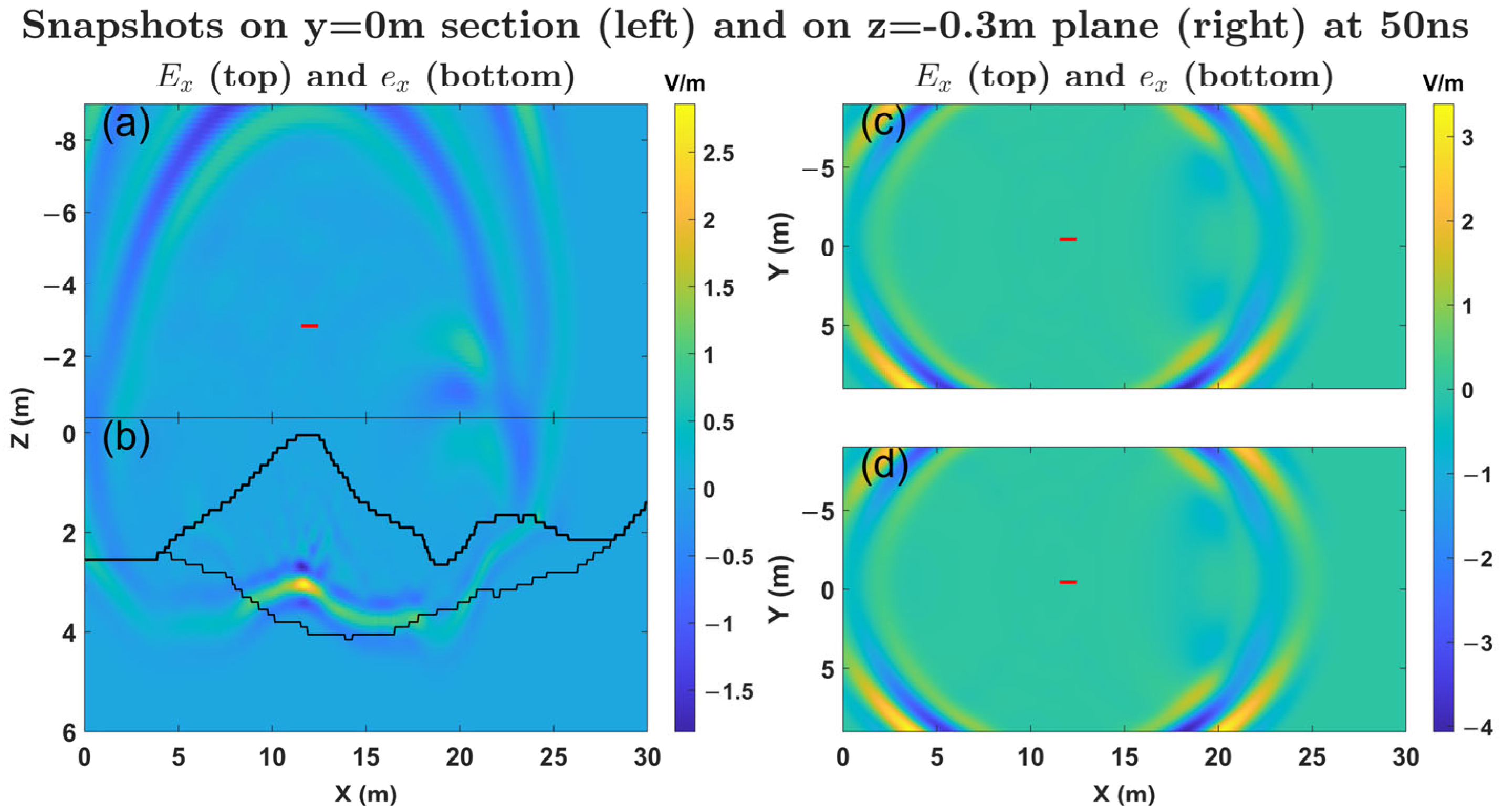
To demonstrate the differences in the propagation of the radar waves within the aforementioned landslide models, the 3D wavefield data were simulated using our subgridding method when the emission source point was at x = 11.55 m. Figure 16 and Figure 17 illustrate the wavefield snapshots at 50 ns for the initial landslide model (Figure 13a) and the landslide model exhibiting fissure development (Figure 13b,c), respectively, with the objective of offering a clear and intuitive comparison of the distinct wavefield features between the two models.

In the wavefield snapshots presented here, the x-axis corresponds to the position of the red dashed line in Figure 13. The x-z section represents the coordinate plane obtained by rotating the original plane 24° counterclockwise. The data used to generate the snapshots consist of the $E_x$ from the CG section (excluding the last layer) and the $e_x$ from the FG section (excluding the first 3 layers). Note that in the x-z section, the z = −0.3 m plane is centrally positioned within the OG region along the z direction, serving as a common boundary line for the two snapshots (the scaled black line in Figure 16 and Figure 17). First, the fields from the coarse and fine grids are graphed separately, employing a consistent color scale. Subsequently, these two images are concatenated together to create the final snapshot of the x-z section. The two subplots on the right respectively present snapshots of the field distribution on the z = −0.3 m horizontal plane, generated using field data from the CGs and the FGs, respectively. The discrete color blocks in the image generated using CG data are more prominent compared to those in the image generated using FG data, highlighting the difference in spatial resolution between the two. Despite this, the snapshots corresponding to the coarse grid and the fine grid exhibit remarkable consistency, with the field values at the junction of the wavefield snapshots remaining continuous and showing no apparent false reflections caused by grid overlap. Due to the relatively high permittivity of the deposit material, the wave propagation speed is slower, and a noticeable delay of the first wave occurs in the accumulation area. At 50 ns, the initial wave is on the verge of crossing the fissure zone, leading to a significantly more complex wavefield distribution within this region (see Figure 17b) when contrasted with the corresponding area in the initial landslide model, which lacks fissures (see Figure 16b). The high permittivity inherent to water-bearing fractures induces a temporal delay in the reflected signal originating from the underlying bedrock surface. This can be substantiated by the time-section diagrams, wherein at the position x = 11.55 m, the temporal values corresponding to point P are recorded as 106.71 ns (as illustrated in Figure 15b) and 102.22 ns (as depicted in Figure 14b), respectively. Consequently, the fracture structure engenders a delay of approximately 3.49 ns in the reflected signal from the subjacent bedrock surface.

3.4. Algorithm Stability Test

The stability of the subgridding FDTD method is influenced by various factors, including grid size, time step size, and the wavefield data communication method at the coarse–fine grid interface, among others. Consequently, many subgridding methods incorporate a filtering operation to suppress the instability introduced by the subgridding scheme [34,36,37]. Unsurprisingly, the stability of most subgridding methods, including ours, is conditional. For instance, the Huygens subgridding method proposed by Bérenger [35] remains stable for up to 1000 time steps. Similarly, the 3D subgridding method [49] demonstrates stability up to 5 × 10⁵ iterations. In contrast, the subgridding method proposed in [50] has been evaluated across multiple models, demonstrating stability even beyond 10 million iterations.

In fact, when the grid step size is relatively small, the time step size must also decrease accordingly, increasing the number of time iterations required to maintain computational stability. This may weaken the correlation between the number of iterations and stability. In contrast, our numerical simulations prioritize minimizing computational memory consumption under the condition of ensuring computational accuracy. This approach leads us to select the largest feasible grid step size and, consequently, the time step size is also relatively large. In this case, the correlation between maintaining computational stability and the number of iterations becomes more significant. In this section, we first evaluate the stability of the subgrid configuration method using a counterexample, followed by a validation of the long-term iteration stability of the proposed algorithm through simulations on a large computational domain.

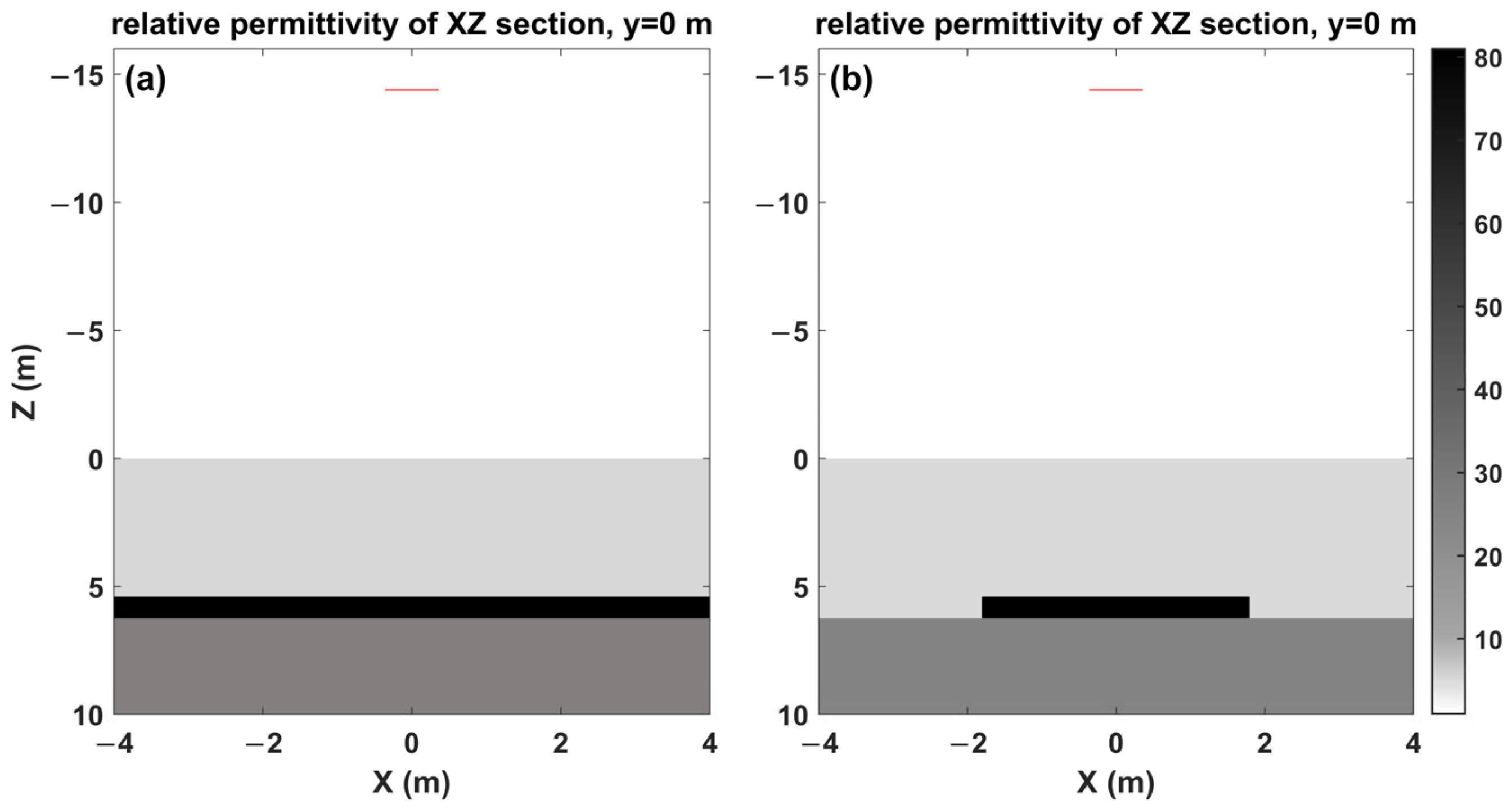
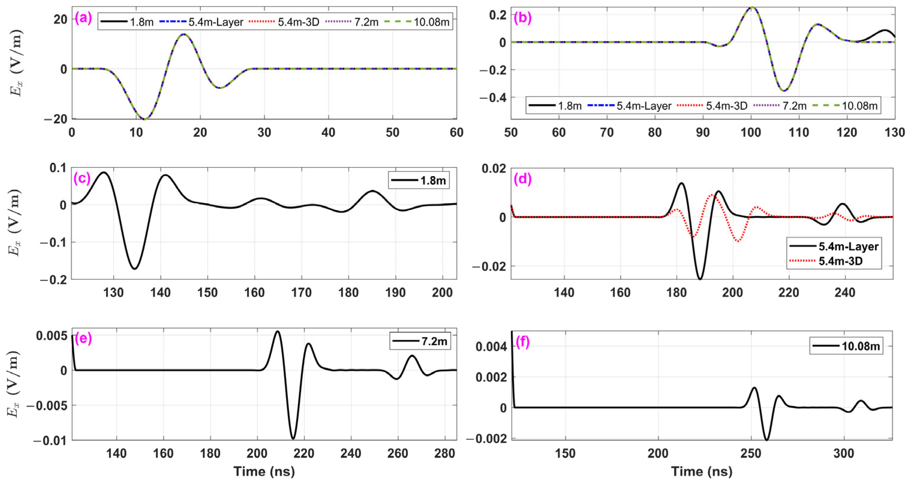
To assess the stability of the proposed method over longer sampling times, we simulated the response of groundwater layer models at various burial depths. The antenna height was set to 14.4 m, with a fixed groundwater layer thickness of 0.84 m and burial depths of 1.8 m, 5.4 m, 7.2 m, and 10.08 m. The water layer had a conductivity of 10 mS/m and a relative permittivity of 81. The overlying medium had a conductivity of 3 mS/m and relative permittivity of 5, while the bedrock medium had a conductivity of 1 mS/m and a relative permittivity of 25. The antenna dimensions were 72 cm × 36 cm × 36 cm, and the excitation current pulse featured a center frequency of 49 MHz with an amplitude of 1 A.

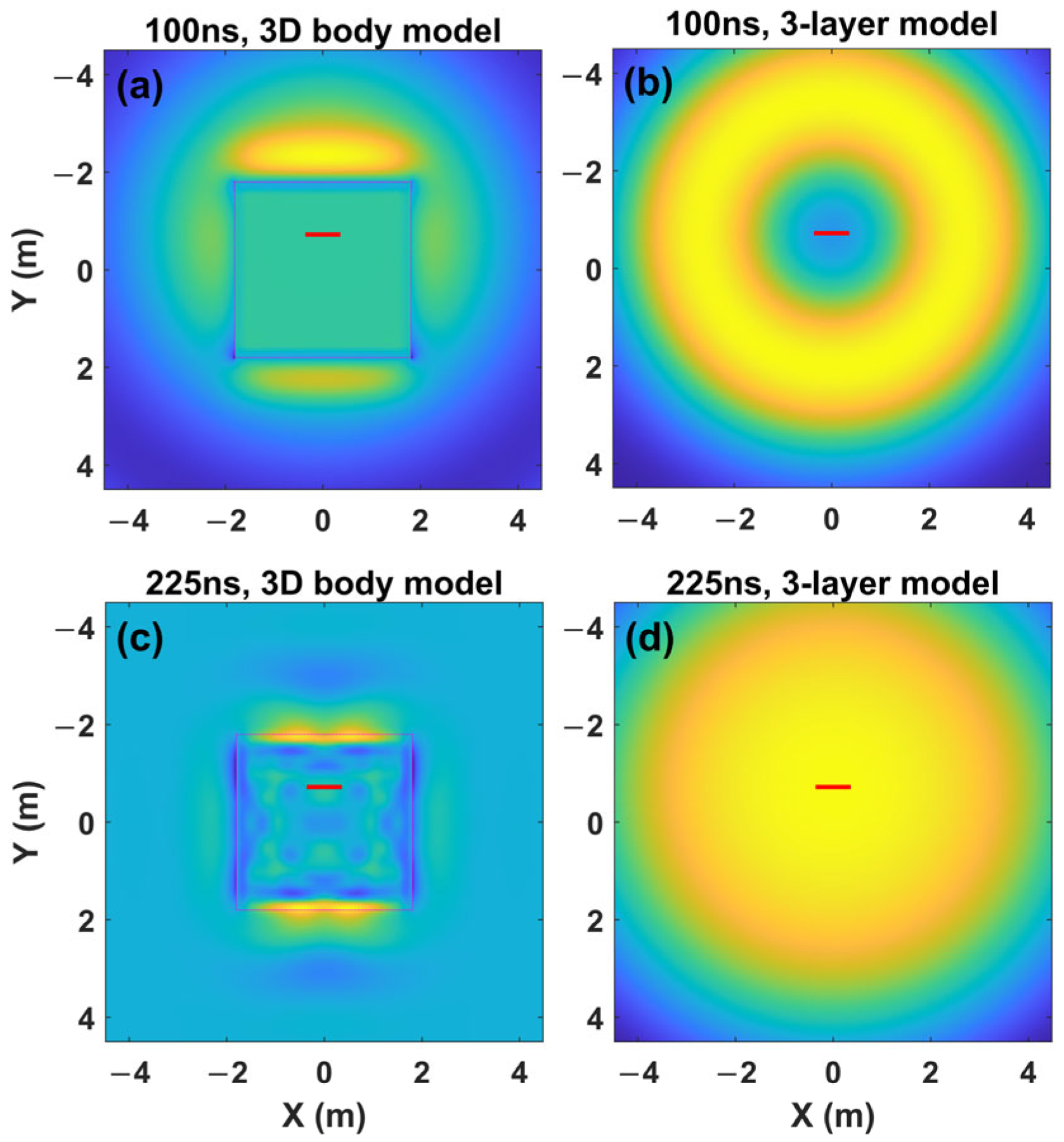
Figure 18a illustrates the distribution of the relative permittivity in the y = 0 m section of the model, with the groundwater layer at a burial depth of 5.4 m. For comparison, Figure 18b presents a model with a 3D water body at the same burial depth. The 3D water body is a thin plate, with a thickness equal to that of the groundwater layer mentioned above and lateral dimensions of 1.8 m × 1.8 m. The excitation source is positioned directly above the 3D water body in the air.

The subgridding method with Nc = 9 was applied in the simulation, where the grid size for the CG in the air layer was 36 cm and the grid size for the FG in the underground layer was 4 cm, with a time step of 0.066 ns. A PML with a thickness of 10 CG cells was placed at the outer boundary of the computational domain. These test models feature large computational domains, resulting in a higher number of iteration time steps. For the model with a groundwater layer depth of 10.08 m, the number of time iterations reached a maximum of 4940.

Table 3. Memory requirement (in GB) for simulating groundwater layer models with different buried depths.

Depth	1.8 m	5.4 m	7.2 m	10.08 m
Standard FDTD	1573.3	2888.8	3796.4	5111.9
FDTD(2,4)	839.63	1524.4	1993.9	2672.5
subFDTD(2,4) − Nc = 9	275.77	392.62	466.99	562.66

presents the memory consumption for simulating groundwater layer methods at various depths of using three models. The memory required by the proposed subgridding method is only 11% to 17.5% of that required by the standard FDTD method and 21% to 32.8% of that required by the standard FDTD(2,4) method. When the burial depth of the water layer exceeds 10 m, the memory demand of the standard FDTD or standard FDTD(2,4) method becomes too large for our server to handle. In such cases, only the proposed subgridding method is capable of completing the numerical simulations.

Figure 19 presents the simulation results for groundwater models at different burial depths. In Figure 19a, the portion before 30 ns corresponds to the direct wave, while the surface reflection wave appears between 96 ns and 120 ns time range in Figure 19b. At this stage, the direct wave and surface reflection wave curves are identical across all models, and the reflection wave from the underground anomaly layer or body has not yet arrived. Figure 19c shows the reflection wave segment for a water layer with a depth of 1.8 m. The reflection wave from the upper boundary of the water layer appears at approximately 123 ns, while the reflection wave from the lower boundary appears at approximately 173 ns. The waveform fluctuation between these two reflections is due to the secondary reflections between the upper boundary of the water layer and the surface, occurring in the time range of approximately 150–174 ns. As the depth of the water layer increases (Figure 19d–f), no secondary reflection waves are observed before the reflection wave from the bottom boundary of the water layer due to the greater distance from the surface. As the burial depth increases, the reflection waves from the upper and lower boundaries of the water layer appear at later times, with their peak amplitudes gradually decreasing, while their waveforms remain similar. The time difference between the reflection waves from the upper and lower boundaries of the water layer in models at different depths remains consistent and aligns with the estimated travel time of radar waves traversing the 0.84 m thick water layer (2×${\displaystyle \frac{0.84}{3/\sqrt{81}}}\times 10=50.4 ns$).

Figure 19d compares the underground interface reflection waveforms of the water layer model (see Figure 18a) and the 3D water body model (see Figure 18b). The maximum amplitudes of the reflection waves from the upper and lower boundaries of the 3D body are 38.72% and 27.09% of those from the water layer model, respectively. Compared to the water layer model, the reflection waveform of the 3D water body is more complex, featuring an additional peak. This complexity, arising from the lateral inhomogeneity of the 3D body, can be clearly illustrated in the snapshots presented in Figure 20.

The grid and time step sizes used in the above calculations are the selected largest possible values that satisfy the CFL condition, significantly reducing computational memory usage and fully demonstrating that our algorithm can successfully perform numerical simulations of water-containing medium models. More importantly, even with a large step size, the response waveform at the maximum time step of 4940 (with a maximum observation time of 326 ns) shows no significant numerical dispersion, confirming the stability of our algorithm. Due to the memory limitations of our server, simulations with larger iteration time steps could not be performed. However, based on the simulation results presented in this section, it is evident that our algorithm can stably compute even more time steps.

4. Discussion

4.1. Major Findings of the Study

The 3D simulation of AGPR is computationally intensive, with memory consumption increasing as flight altitude and subsurface permittivity rise. To enable 3D simulations on an ordinary server, we sought to maximize the grid size to economize on computational memory. To achieve this, we utilized a high-order FDTD method, which permits larger grid steps compared to standard FDTD approaches. However, this strategy alone did not meet our objectives. Therefore, we integrated a subgrid technique alongside the high-order FDTD, deploying high-order finite differences across both coarse and fine grid regions to significantly reduce computational memory demands. This enabled the 3D simulation of landslide models with practical relevance. Despite this, the extended stencil inherent to high-order finite differences posed challenges in data exchange between coarse and fine grids within the subgrid framework. To address this, we developed a sophisticated subgrid architecture that integrates overlapping coarse and fine grids with virtual grids, ensuring accurate field value updates at each node using the high-order FDTD method. Additionally, to mitigate the challenges posed by the long stencil, we introduced strategies to facilitate the smooth transition of fields between nodes of differing grid sizes, reducing numerical dispersion errors, especially when crossing medium boundaries in overlapping zones.

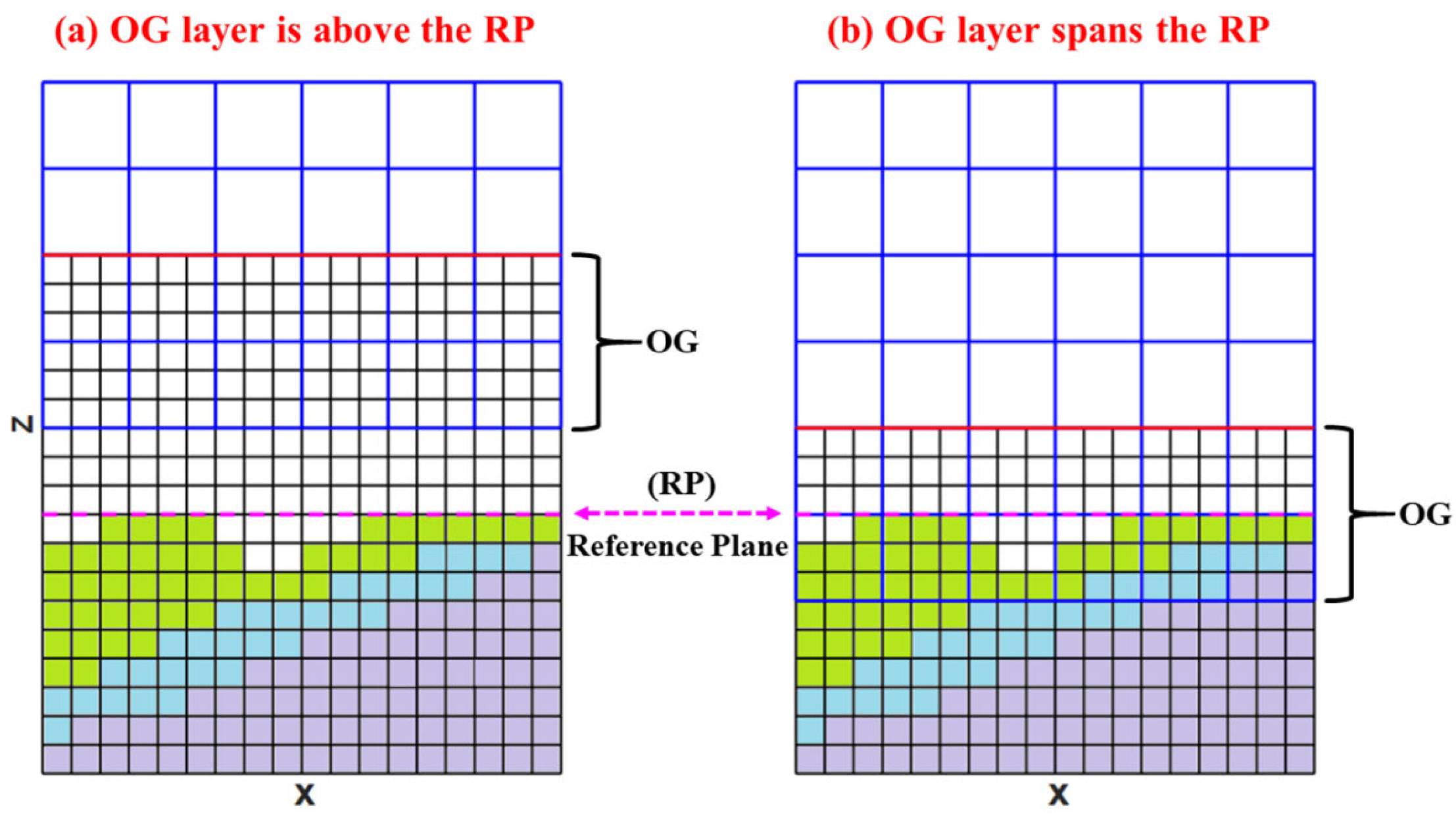
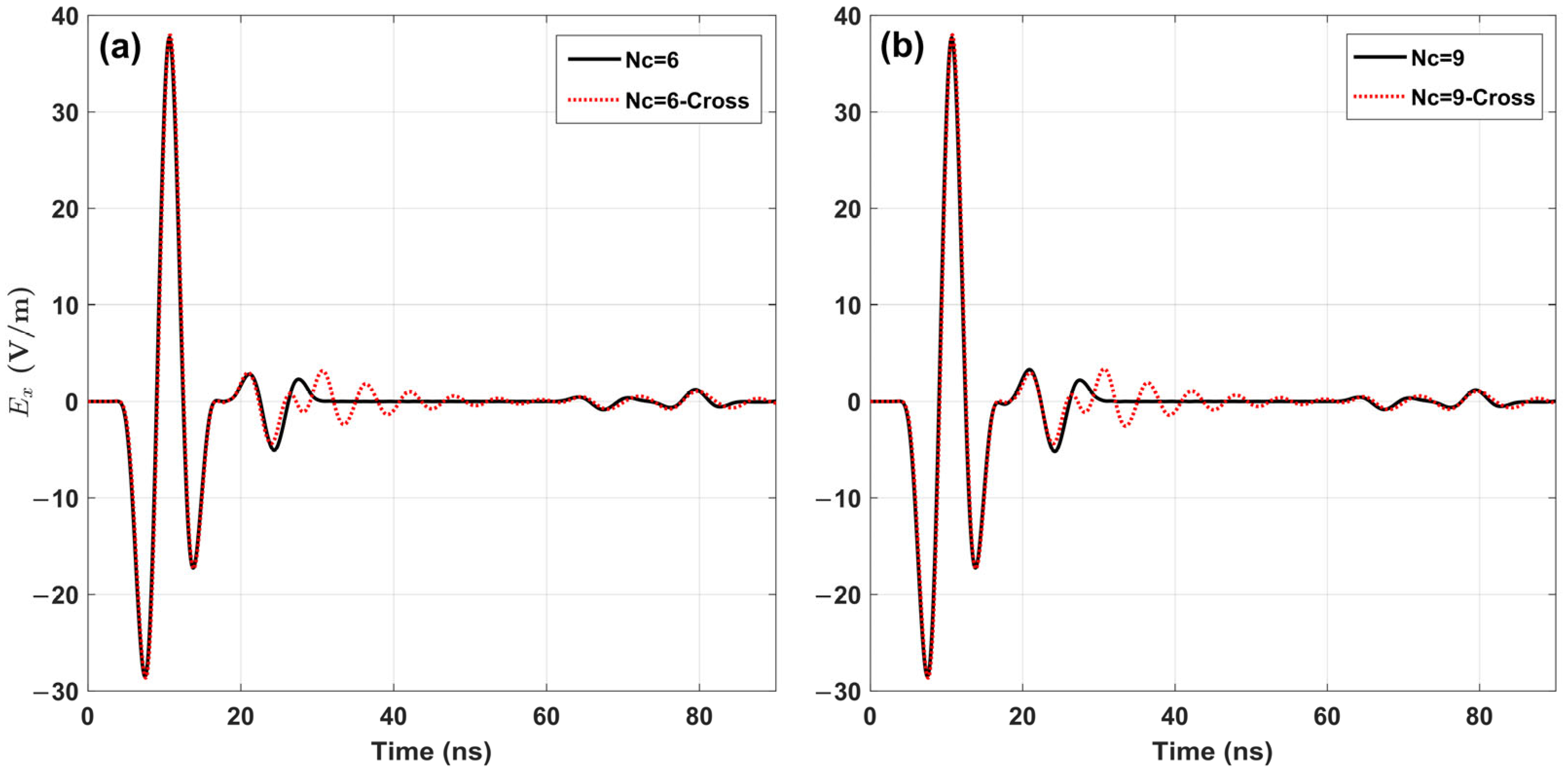
Without adopting the subgridding configuration proposed in this article, memory savings cannot be realized, and the results may suffer from oscillations or even divergence. For instance, when the overlapping grid extends across the surface, as shown in Figure 3b, noticeable oscillations emerge in the computed results. The simulation experiment comparing two subgrid configurations (see Figure 3) was tested using the WBSL model (shown in Figure 21). The response curves produced by the mesh configuration from Figure 3b exhibit oscillations after approximately 25 ns, regardless of whether the GRF was set to 6 or 9. This behavior mirrors oscillations observed in previous studies [37], where an isotropic spatial filter was introduced to suppress such effects. The response curves generated by the mesh configuration in Figure 3b display more pronounced and prolonged oscillations. This is due to the overlapping grids with media having significantly different electrical properties—specifically, a lossy underground medium and air. In high-order difference calculations, transitioning between these two media introduces errors, which are subsequently amplified by the subgrid approach. In contrast, the response curves from our proposed subgrid configuration (Figure 3a) show no oscillations and require no additional filtering. This comparison not only validates the effectiveness of the subgrid approach presented here but also emphasizes the importance of well-designed subgrid configuration and an efficient data exchange mechanism between coarse and fine grids to ensure accurate high-order difference calculations.

4.2. Significance of the Research Findings

The proposed method achieves substantial memory savings while maintaining high-order accuracy in both coarse and fine grid regions. Using an ordinary server, we conducted simulations on a model with a flight altitude of up to 14.4 m and a maximum groundwater layer depth of 10.08 m. To the best of our knowledge, this represents the largest-scale 3D numerical simulation of AGPR conducted to date. The method offers significant practical value, enabling simulation on a much larger scale than standard FDTD methods, making it particularly suitable for modeling real-world landslides. As shown in Figure 13, the simulated landslide model spans over 30 m in length, with the bedrock surface depth exceeding 4 m. More importantly, our method can handle arbitrarily complex models, overcoming a key limitation of traditional subgridding FDTD methods, which are typically restricted to localized anomalous target regions [33,35,38,39,40]. These advantages enhance the versatility and applicability of our approach. Higher flight altitude results in a greater proportion of the computational domain using coarse grids, while higher subsurface permittivity increases the number of computational grids and time steps required. While these factors often exceed the capabilities of ordinary servers, the proposed method effectively mitigates these challenges, enabling successful simulations under such demanding conditions.

This study introduces a novel advancement in subgridding FDTD methods by implementing high-order FDTD schemes across both coarse and fine grid regions—an achievement not realized by previous subgridding FDTD methods. This innovation is particularly significant because the extended stencils of high-order FDTD schemes pose substantial challenges in data computation and communication near the boundaries between coarse and fine grid regions. Our method effectively resolves these challenges, ensuring high-order accuracy in both regions. Additionally, by employing larger grid sizes and correspondingly larger time step sizes, our simulation method significantly reduces computational resource demands (see Figure 8 and Table 2).

4.3. Comparison with Previous Studies

The literature on the 3D forward modeling of AGPR remains limited. Using our approach, we successfully conducted the first 3D simulation of large-scale AGPR detection for complex geological landslide structures. The methodology presented here marks a significant departure from previous subgrid FDTD techniques in several key areas. First, earlier studies primarily focused on localized target models, where fine grids were applied only to a specific target area while coarse grids were used for surrounding regions. Our method imposes no such limitations. Unlike previous approaches, which were confined to localized target models, our method can be applied to arbitrarily complex structural models without constraint. Second, our algorithm introduces a major advancement by employing high-order FDTD methods across both fine and coarse grid regions. This allows for the use of larger grid sizes in both areas, significantly reducing memory requirements. In contrast, most prior studies relied on standard FDTD methods in both fine and coarse grids, with only basic wavefield data interaction between them. Some subgrid algorithms have been proposed based on hybrid methods. For instance, studies [38,39,40] introduced a two-dimensional subgrid algorithm that applied standard FDTD methods in the local FG region and high-order finite-difference methods in surrounding CG regions.

In comparison, our method employs long-stencil high-order finite differences for wavefield iteration updates across both fine and coarse grid regions. This improvement directly results from our carefully designed and optimized grid configuration, ensuring a seamless transition between coarse and fine grids. This approach enables the use of larger grid steps in both regions (in this study, we employ grid sizes twice as large as those used in standard FDTD methods), achieving significant savings in computational memory while maintaining high-order accuracy. Additionally, the enhanced computational efficiency of our method enables the large-scale simulation of geologically realistic landslide models using an ordinary server—something existing methods cannot achieve. This breakthrough bridges the gap between theoretical modeling and practical, real-world applications.

4.4. Challenges and Future Research Directions

Since our simulation framework accommodates models with arbitrary structural distributions rather than the localized target area models utilized in previous methods, our subgrid regions inherently include the PML boundaries. Consequently, the subgrid algorithm must also be applied within the PML to maintain a uniform thickness across both coarse and fine grid regions. However, when using a relatively large GRF (e.g., Nc = 9), the fine grid region is compelled to incorporate multiple layers of fine-grid PMLs. This may exceed the actual absorption boundary requirements, leading to unnecessary computational overhead. Therefore, greater consideration should be given to the design of the PMLs’ thicknesses. While we have conducted multiple tests to refine this aspect, further improvements are still needed.

Moreover, in certain specialized models with uniform medium layers, significant variations in permittivity may exist across different regions. To address this, the proposed method can be extended to a subgridding scheme based on a multi-grid technique, where the FGs are used only in high-permittivity regions, while lower-permittivity regions have relatively larger grid sizes. This optimization can further reduce computational memory consumption. These are promising directions for future research.

In summary, this study introduces a novel subgridding method that effectively employs high-order FDTD schemes in both coarse and fine grid regions, significantly saving memory while maintaining high-order accuracy. Our approach overcomes key challenges in subgrid data exchange and numerical dispersion, imposes no restrictions on the simulation model, and is highly suitable for 3D AGPR simulations of complex landslide models. The findings demonstrate the feasibility of conducting 3D numerical simulations of landslide models on standard servers, paving the way for more accurate and computationally efficient AGPR 3D simulations in studies of complex structural models.

5. Conclusions

In this article, we propose a novel subgridding scheme combining the higher-order finite-difference time-domain (FDTD) method, where both the coarse and fine grids utilize the FDTD(2,4) approach. For this reason, larger grids can be employed in both coarse and fine mesh regions, and this method drastically reduces the computational memory consumption required for a three-dimensional (3D) landslide forward modeling of Airborne Ground-Penetrating Radar (AGPR). When the model contains a medium with high permittivity, such as water, the huge memory requirement of the standard FDTD method makes it impossible to simulate it on an ordinary server. The higher the altitude of AGPR in the air, the more advantages this method has in reducing memory consumption in 3D forward modeling. The configuration of the overlapping regions of coarse grids and fine grids and the weighting correction of the fields at the nodes in overlapping grids are very necessary to ensure the correctness and stability of the calculation results. These measures are successfully verified by the subgridding scheme with different grid refinement factors (GRFs), while the results of the traditional scheme without the above measures oscillate. In fact, in our subgridding algorithm, the GRF can be either odd or even, and the most suitable factor can save more computing resources than others. Wavefield snapshots demonstrate that the transition region between the coarse and fine grids is smooth, with no spurious reflections caused by the different grid systems, fully verifying the reliability of the proposed algorithm. In contrast to conventional local subgridding configurations, our scheme eliminates the restriction of being applicable solely to local target models. It is tailored for models with arbitrarily complex layered structures, offering practicality and versatility. Hence, the proposed subgridding FDTD(2,4) method can serve as an adaptable and practical tool for simulating the wave field of AGPR, particularly when the model has a high permittivity medium in it, as seen in landslide models with groundwater.

The simulation results suggest that as the flight altitude increases, the amplitudes of the reflected waves from both the surface and the subsurface bedrock interface decrease. However, within the total reflected wave energy from the two interfaces, the proportion of energy originating from the deeper bedrock interface increases. Therefore, as long as the effective reflection signals from underground structures have a sufficient signal-to-noise ratio, the airborne-based GPR may be more advantageous than the ground-based GPR, especially in rugged surface environments. In this case, appropriately increasing the flight altitude may be beneficial for detecting deeper subsurface interfaces. Additionally, we simulated the time-domain section of the responses (B-scan image) through a deposition-type landslide model with a bedrock depression and explained the formation of reflected wave events using wavefield snapshots. The B-scan image clearly displays the bedrock structural features, demonstrating that AGPR is an effective tool for exploring shallow, complex structures. It also highlights the effectiveness of our 3D forward modeling method, which can perform simulation on ordinary servers and provides a reliable support for data interpretation of AGPR.