Article

Evaluation of Sentinel-2 Deep Resolution 3.0 Data for Winter Crop Identification and Organic Barley Yield Prediction

by
Milen Chanev
,
Ilina Kamenova
,
Petar Dimitrov
and
Lachezar Filchev
*
Space Research and Technology Institute, Bulgarian Academy of Sciences (SRTI-BAS), 1113 Sofia, Bulgaria
*
Author to whom correspondence should be addressed.
Remote Sens. 2025, 17(6), 957; https://doi.org/10.3390/rs17060957
Submission received: 31 January 2025 / Revised: 5 March 2025 / Accepted: 7 March 2025 / Published: 8 March 2025
(This article belongs to the Section Remote Sensing in Agriculture and Vegetation)

Abstract

:
Barley is an ecologically adaptable crop widely used in agriculture and well suited for organic farming. Satellite imagery from Sentinel-2 can support crop monitoring and yield prediction, optimising production processes. This study compares two types of Sentinel-2 data—standard (S2) data with 10 m and 20 m resolution and Sentinel-2 Deep Resolution 3 (S2DR3) data with 1 m resolution—to assess their (i) relationship with yield in organically grown barley and (ii) utility for winter crop mapping. Vegetation indices were generated and analysed across different phenological phases to determine the most suitable predictors of yield. The results indicate that using 10 × 10 m data, the BBCH-41 phase is optimal for yield prediction, with the Green Chlorophyll Vegetation Index (GCVI; r = 0.80) showing the strongest correlation with yield. In contrast, S2DR3 data with a 1 × 1 m resolution demonstrated that Transformed the Chlorophyll Absorption in Reflectance Index (TCARI), TO, and Normalised Difference Red Edge Index (NDRE1) were consistently reliable across all phenological stages, except for BBCH-51, which showed weak correlations. These findings highlight the potential of remote sensing in organic barley farming and emphasise the importance of selecting appropriate data resolutions and vegetation indices for accurate yield prediction. With the use of three-date spectral band stacks, the Random Forest (RF) and Support Vector Classification (SVC) methods were used to differentiate between wheat, barley, and rapeseed. A five-fold cross-validation approach was applied, training data were stratified with 200 points per crop, and classification accuracy was assessed using the User’s and Producer’s accuracy metrics through pixel-by-pixel comparison with a reference raster. The results for S2 and S2DR3 were very similar to each other, confirming the significant potential of S2DR3 for high-resolution crop mapping.

1. Introduction

Due to their rational use of resources, farmers significantly impact the shaping of the natural environment. This has significantly influenced the formation of cultural ecosystems and the provision of ecosystem services in rural areas, including healthy and safe food, soil, air, surface water quality, biodiversity, and rich landscapes [1,2,3].
Organic farming is a specific form of agriculture that protects the environment and biodiversity and provides healthy, high-quality, and safe food. For this reason, organic farming is characterised by greater natural environment diversity than conventional agriculture [4,5]. Organic farming serves several functions: it provides food grown without pesticides and herbicides, while simultaneously offering numerous economic, environmental, and social benefits, thus making agribusiness more sustainable [6]. The sustainability of organic farming is a key focus in agricultural development [7]. Environmental care and health concerns are among the main motivations for consumers to seek food produced using organic farming methods. On the other hand, there is growing ecological awareness and a shift towards eco-friendly consumption patterns, which necessitates the development of organic production and is associated with an increasing demand for such foods [8].
Satellite data are increasingly proving to be a suitable tool for agricultural crop monitoring. This type of data can be used to support organic food and feed production. Research and technological advances in remote sensing have significantly improved our ability to detect and quantify the physical and biological loads that affect crop productivity [9]. Data from the Sentinel-2 (S2) satellite have been successfully used to distinguish between different types of farming systems, such as conventional, organic, or biodynamic [10]. The crop yield is perhaps the most important information for crop management in precision agriculture, which is of interest not only to farmers but to several public and private organisations [11,12,13,14]. In general, remote sensing technology provides an alternative method for estimating crop yields. The other advantage of data from the Sentinel-2 satellite is that they provide an opportunity to develop an easier and more accurate modern method for monitoring the yields of different crops in organic farming. In addition, this type of data provides an opportunity to determine the quantities of food supplies [14]. Data from S2 are a valuable resource for Earth observation, providing multispectral images with spatial resolutions of 10, 20, and 60 m, which in some cases may be insufficient. This issue can be addressed with better-resolution data [15,16]. Increasing the spatial resolution of satellite data using artificial intelligence is of great interest to remote sensing experts. It offers the possibility of data with improved spatial resolution [17]. A problem closely related to yield estimation is crop type mapping. Accurate maps of the distribution of individual crops are needed for applying crop-specific yield models, estimating crop acreage, and, in general, providing data in support of monitoring and informed decision-making [18]. Sentinel-2 Deep Resolution 3 (S2DR3) represents a model that increases all 12 spectral bands of a single Sentinel-2 L2A scene from the original 10 × 10 m, 20 × 20 m, and 60 × 60 m for a pixel spatial resolution of up to 1 × 1 m. The model is made in a way that allows the fine spectral variations in soil and vegetation in all 12 multispectral channels of Sentinel-2 to be preserved. This model, introduced in [19], leverages deep learning techniques to improve image quality and information content significantly. The enhanced resolution allows for more detailed analysis and better decision-making in various applications, such as agriculture, urban planning, and environmental monitoring.
Super-resolution imaging in remote sensing has gained significant attention due to its ability to enhance the spatial resolution of satellite images. Ref. [20] provides a comprehensive overview of super-resolution techniques tailored explicitly for remote sensing applications. Its authors’ work highlights the importance of reconstruction accuracy compared to ground truth rather than merely generating visually attractive outcomes. The book discusses various approaches, including single-image super-resolution (SISR), multi-image fusion, and task-driven super-resolution.
SISR tries to predict and reconstruct a high-resolution image from a degraded, low-resolution image, where the image degradation process is unknown (in an actual situation) and complex [21,22,23]. The method finds applications in different fields, including remote sensing [24,25]. The effectiveness of SISR models like S2DR3 has been demonstrated in numerous studies, showing the increased spatial resolution, reduced entropy, and improved information content of super-resolved images. These models have been successfully applied to large-scale commercial projects, covering millions of square kilometres over the past few years. Integrating deep learning and satellite hardware optimisation has further enhanced the performance of these models, making them a valuable tool for Earth observation and remote sensing.
This study aimed to evaluate the performance of Sentinel-2 Deep Resolution 3 images compared to standard Sentinel-2 in two agricultural applications: (i) predicting the yield of organic barley and (ii) mapping winter crops.

2. Materials and Methods

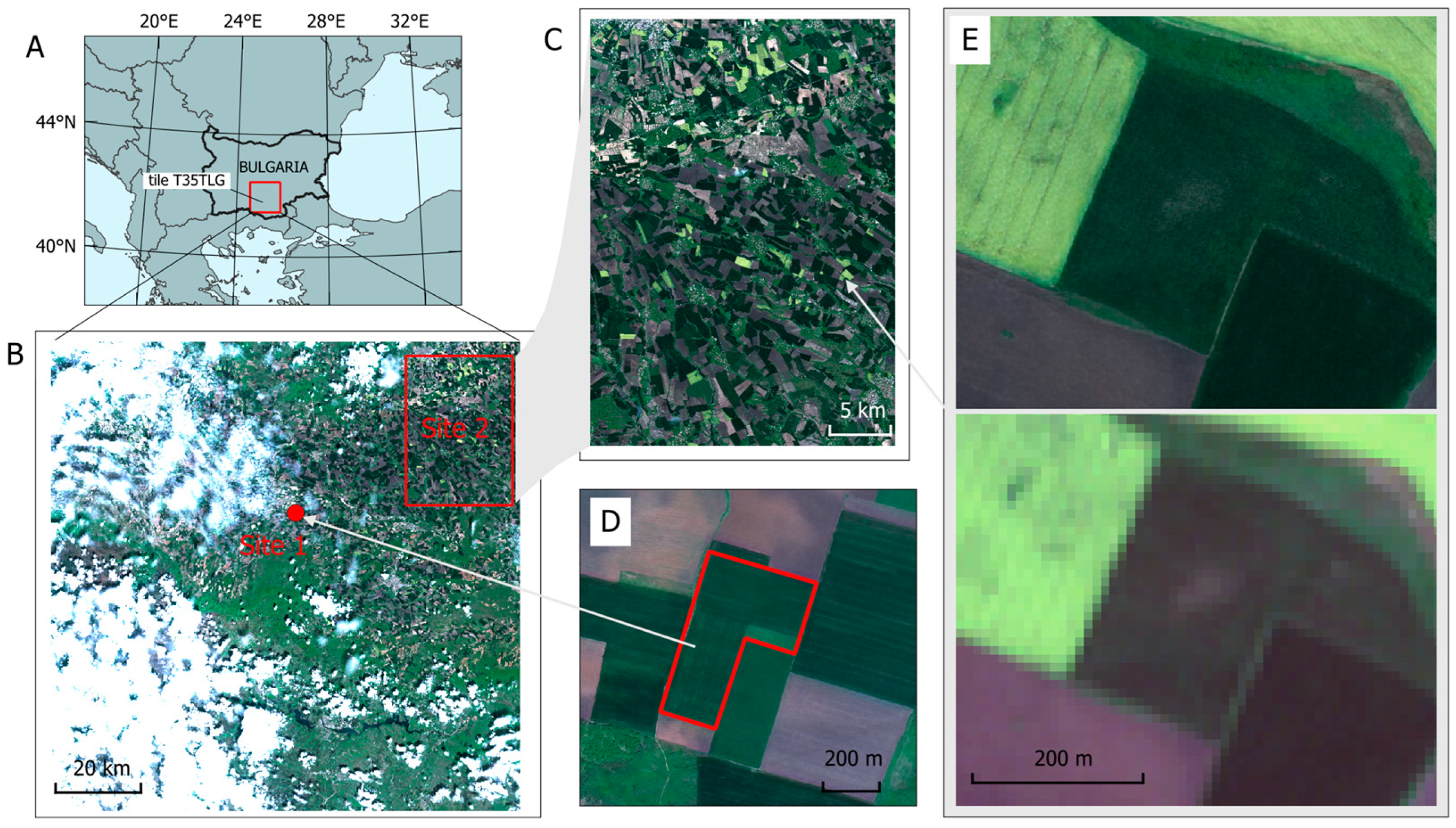
2.1. Study Sites and Satellite Image Datasets

For the aims of this study, two sites, corresponding to the two sub-objectives, were selected, both located in the Upper Thracian Lowland in southern Bulgaria (Figure 1A). This region is one of the most important agricultural areas of the country, producing a diversity of crops, including grains, oil plants, rice, vegetables, grapes, etc. Most of the lowland is in the hypsometric belt between 100 and 300 m a.s.l. The main soil types are Vertisols (Smolnitsa), Fluvisols, and Planosols [26,27]. Concerning the climate, the area is located at the southernmost extreme of the continental temperate region of Europe and shows transitional characteristics of the Mediterranean climate. The annual precipitation is about 500–600 mm, the mean temperature in January is between 0 and +1 °C, and the mean temperature in July is 22–24 °C [28,29]. The first site (Site 1) was an organically certified barley field (area: 17.2 ha; Figure 1D). In this field, ground data for crop yield were collected. The field was sown in the fall of 2022 with the barley crop. The second site (Site 2) represented an artificially defined region of 25 km × 35 km where crop classification was performed (Figure 1C). The location of this site was determined to avoid clouds in the available satellite imagery and to cover, as much as possible, continuous tracts of arable land with few settlements and other land use types.
Four Sentinel-2 Deep Resolution 3.0 (S2DR3) images with 1 m spatial resolution were provided by DigiFarm Norway (Table 1). The S2DR3 data are produced on demand by processing the original Sentinel-2 datasets and are delivered using the same tiling grid as Sentinel-2. This study used data for tile T35TLG, which covered both study sites (Figure 1B). As some of the images had significant cloud cover, we had to select the crop classification site to maximise the number of useful images. Nevertheless, the 15 April 2023 image was unusable for classification (Table 1). The original Sentinel-2 imagery (10 and 20 m spatial resolution) corresponding to the S2DR3 products was downloaded from the Copernicus Browser website (https://browser.dataspace.copernicus.eu/ (accessed on 7 January 2025)) Examples of RGB images of the two types of images are shown in Figure 1E.

2.1.1. Barley Yield Data

Phenological observations and yield sampling were conducted in the barley field in Site 1 (Figure 1D) in the agricultural year 2022–2023. The registration of the main phenological phases was based on the following scale: BBCH-BBCH-41—early boot stage; BBCH-51—beginning of panicle emergence; and BBCH-77—late milk [30]. The onset of each phase is when 25% of the plants have entered it. Reporting occurs when 75% of plants are in the relevant phase. In the EOS Crop-monitoring platform, in the phenological phase tillering BBCH-21, three pixels were selected in the field with NDVI values of 0.8, 0.7, and 0.6, respectively. The pixels are 20 × 20 m, and a sample site with dimensions of 10 × 10 m is organised in each. Upon the plants reaching the technological maturity phase BBCH-99 at the four ends of the trial site, the GPS coordinates of all 4 m sized 0.25 × 0.25 m plants were collected. Biometric studies were conducted using Shanin’s methodology (1977) [31]. Before harvesting, all plants of 0.25 × 0.25 m in 4 replicates were taken for the three different NDVI values. In each metre, all plants were counted, and for 25 plants, the following indicators were tracked: plant height (cm); class length (cm); grains in the class (number); grain mass in the class (g); biological yield (kg/da); physical qualities of the grain; and mass per 1000 grains (g) for four replicates.

2.1.2. Crop Type Data

Crop type information for Site 2 was obtained for 2023 from geospatial application (GSA) data collected from the Integrated Administration and Control System (IACS). The IACS is used by European Union (EU) countries to manage, monitor, and control all area- and animal-based common agricultural policy (CAP) interventions and to ensure that comprehensive and comparable data are available throughout the EU [32]. The GSA data comprise georeferenced agricultural parcels for which farmers have applied for aid in vector format. Individual farmers manually define the parcels (based on reference vector and image data) and provide information about the crop sown in each of them in the current agricultural year.

2.2. Methods

2.2.1. Correlation of Yield with Vegetation Indices

In the GIS environment, the pixel values for each of the sample sites in the field were extracted from the generated vegetation indices (VIs) for the investigated field by satellites S2 and S2DR3. The following vegetation indices (see Table 2) were used in this study: GCVI, NDRE2, NDRE1, NMDI, DVI, CCCI, NDWI, EVI2, OSAVI, EVI, NDVI, SR, and TO. The methods of calculation were taken from the index database. Then, maps were drawn up on the field with the corresponding VI. In the next step, yield maps for the field under investigation were compiled from the generated VI and yield data. The software with which the processing of the data received from satellite S2 and S2DR3 was carried out is ArcGisPro v3.4.
The correlation analysis for the statistical proof of the most suitable use of a VI was conducted in MS EXCEL. It was assumed that when the correlation coefficient (r) is from 0 to 0.33, the correlation is weak; when r is in the range from 0.34 to 0.66, it is average; and from 0.67 to 0.99, it is strong [46].

2.2.2. Crop Classification

Pixel-based classification was performed to map the three main winter crops in Site 2, i.e., wheat, barley, and rapeseed. These crops were selected because their area accounted for 50% of the agricultural land in Site 2 and because available images coincided with their growing season—from early March, when the renewal of growth after the winter occurs, to early June, when ripening begins. To exploit the full potential of the image datasets, one multitemporal image stack was generated and classified for each type of data, S2 and S2DR3. The stacks included the three cloud-free images taken over Site 2 (Table 1) and had 27 bands, 9 from each date. The bands included were B02, B03, B04, B08, B05, B06, B07, B11, and B12 (for information about Sentinel-2 bands, the reader is referred to [47]). The S2 stack adopted the spatial resolution of the finer bands (10 m), with the rest being resampled accordingly. The S2DR3 stack retained the native image resolution of 1 m.
A total of 2672 IACS/GSA fields (wheat: 2188; barley: 351; rapeseed: 133) with areas between 0.1 and 225.9 ha (mean: 10.9 ha; median: 4.2 ha) were available. The fields were divided into five mutually exclusive folds at random. For each image dataset, five classifications/maps were performed/generated, whereby the fields of one fold were used as an inclusion mask to define the mapping area, while the other folds were used to extract training data for the classifier. This iterative procedure allows the full area to be classified while, at the same time, no training pixels are used from the fields being classified. It also permits the accounting of sampling errors and provides more insight into the classification of performance variability. The training data were extracted using a stratified sample of 200 points per crop, applying an inward buffer of 20 m to the fields and defining points to be no closer than 200 m to each other. The same point datasets per iteration were used for the two image datasets for a better comparability of results. The classification was performed with the plugin EnMAP-Box v3.15.3 in QGIS v3.34.6 [35], using two methods, Random Forest (RF) [46] and Support Vector Classification (SVC) [48] with the Radial Basis Function kernel. The parameters of both classifiers were optimised using a cross-validated grid search procedure using the training data. This was carried out separately for each of the folds described above. The optimised parameters and candidate values are shown in Table 3. To evaluate the S2 and S2DR3 classifications, two rasterised versions of the IACS/GSA fields were used, with a spatial resolution of 10 m and 1 m, respectively. The classifications produced in the five iterations were evaluated individually by pixel-by-pixel comparison with the reference raster over the full extent of the fields in the corresponding fold. The User’s and Producer’s accuracies for the three crop classes were calculated based on the error matrix [48], where the User’s accuracy of class i is the number of pixels correctly labelled by the classifier as class i divided by the number of all pixels classified as class i, while the Producer’s accuracy of class i is the number of pixels correctly labelled by the classifier as class i divided by the number of all pixels which belong to class i according to the reference raster.

3. Results

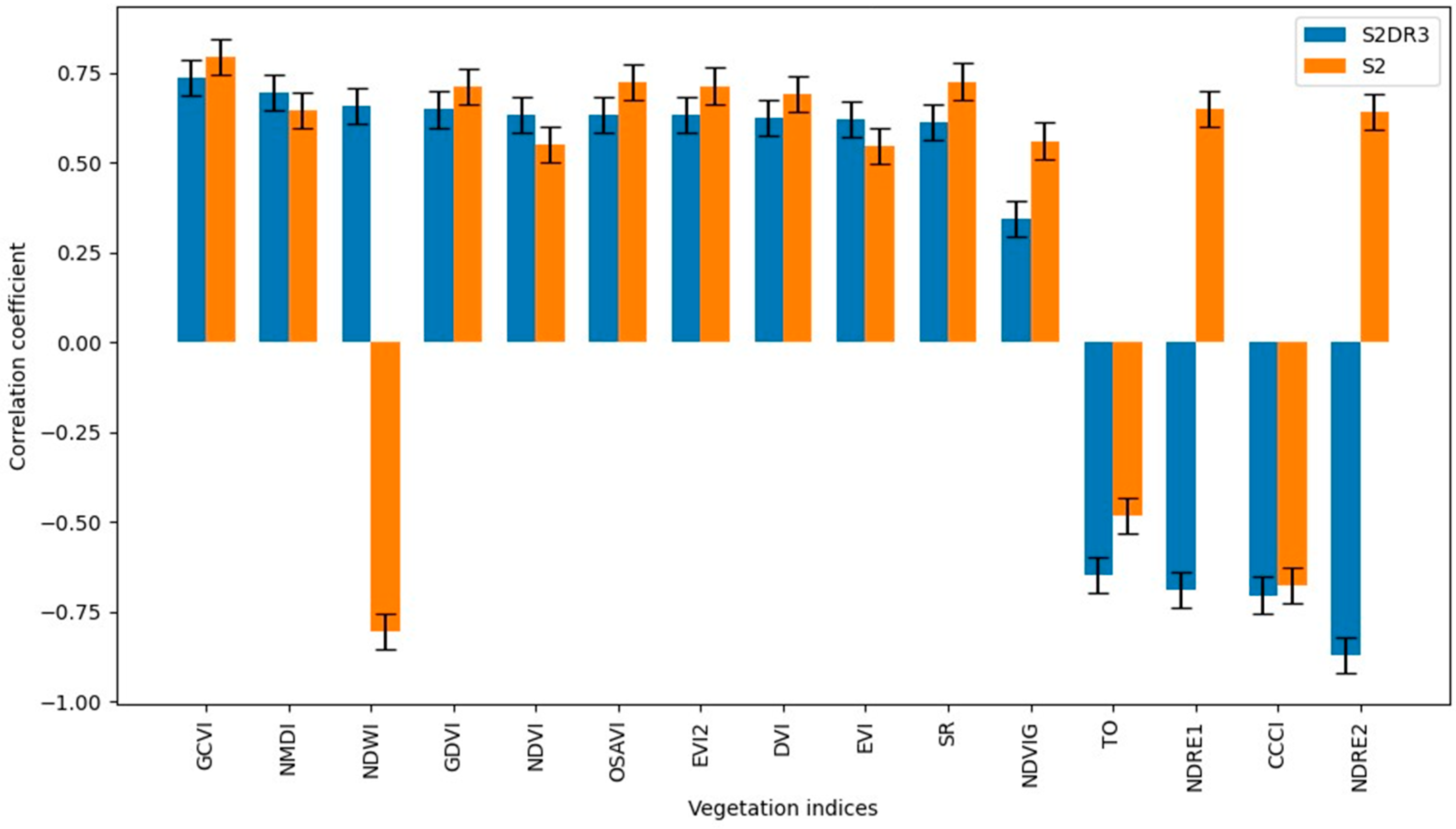
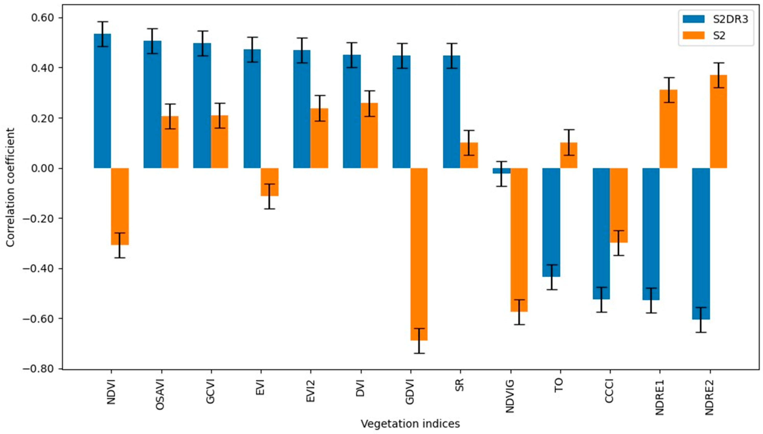
3.1. Results of the Correlation Between Crop Yield and Vegetation Indices

This study aims to test and compare the application of the S2DR3 model against Sentinel-2 L2A for monitoring yields in barley crops grown under organic farming conditions. In addition, it aims to establish which phenological phases are most appropriate to use for the S2DR3 data. Figure 1 shows the correlation relationships between S2 and S2DR3 VI and the yields from the organic barley in BBCH-41, the early boot stage. It is clear from the diagram that in terms of yields, 12 of the VIs have a positive correlation relationship, and 3 have a negative correlation relationship. It is noteworthy that of the 15 CAs that have a positive correlation, 6 of them have a strong positive correlation; these are, respectively, GVI (r = 0.80), SR (r = 0.73), OSAVI (r = 0.73), EVI2 (r = 0.71), GDVI (r = 0.71), and DVI (r = 0.69). The highest negative correlation is for the NDWI (r = −0.80).
Figure 2 shows the correlation relationships between S2DR3 and S2 VI and the yields from the organic barley in BBCH-41, the early boot stage. From the data analysis, it is clear that 10 of the VIs have a strong correlation with the yield, and the GCVI has the highest correlation (r = 0.74), while the NDVIG VI has the lowest (r = 0.35). It should be noted that the NDWI generated from S2DR3 data has a strong positive correlation with yield (r = 0.66), while that generated from S2 has a strong negative correlation with yield (r = −0.8). The following S3DR3 VIs have strong but negative correlations with yield: TO (r = −0.65), NDRE1 (r = −0.69), CCCI (r = −0.7), and NDRE2 (r = −0.87). In this phase, the VIs NDRE1 and ENDRE2 generated from data from S2 show an average correlation with yield, with (r = 0.65) and (r = 0.64), respectively. It is noticeable that the data from S2DR3 VIs in this phase show similarity with the data from S2.
Figure 3 presents the results of the correlation analysis between VIs generated from S2DR3 and S2 data in phase BBCH-51, the beginning of panicle emergence, and the organic barley yield. A ratio of correlations between S2 VIs and yields in this phase makes it clear that in this phase, 10 of the generated VIs are correlated with yields. Still, a decrease in correlation is found compared to the previous phase, and the highest correlation with yield is for ENDRE2 (r = 0.62). The following VIs have strong negative correlations: TO (r = −0.48), CCCI (r = −0.49), and NDWI (r = −0.57). VIs generated by the S2 satellite, namely, CCCI (r = −0.49) and NDWI (r = −0.57), are negatively correlated with organic barley yield.
From the data in Figure 3, it can be seen that of the VIs generated from S2DR3 data, 12 are strongly positively correlated with yields, and only VI TO is strongly negatively correlated (r = −0.68). It can be said that at this stage, the data from S2DR3 show better possibilities for predicting organic barley yields.
Figure 4 presents the results of the correlation analysis between the VIs generated from data from S2DR3 and S2 in BBCH-77, the late milk phase, and the yield of organic barley. From the presented data, it can be seen that eight of the vegetation indices generated from S2DR3 data have an average positive correlation with the yields of organic barley. In this phase, the NDVIG VI (r = −0.02) does not have any correlation with yields. Four of the VIs (TO r = −0.43; CCCI r = −0.52; ENDRE1 r = −0.53; and ENDRE2 r = −0.60) have an average negative correlation with organic barley yields. In this phase, the data from S2DR3 and the NDVI (r = 0.53) are the most suitable for predicting yields. The vegetation indices generated in this phase from data from the S2 satellite are not suitable for determining and predicting the yields of biological barley, as only VI NDRE2 (r = 0.37) has an average positive correlation.

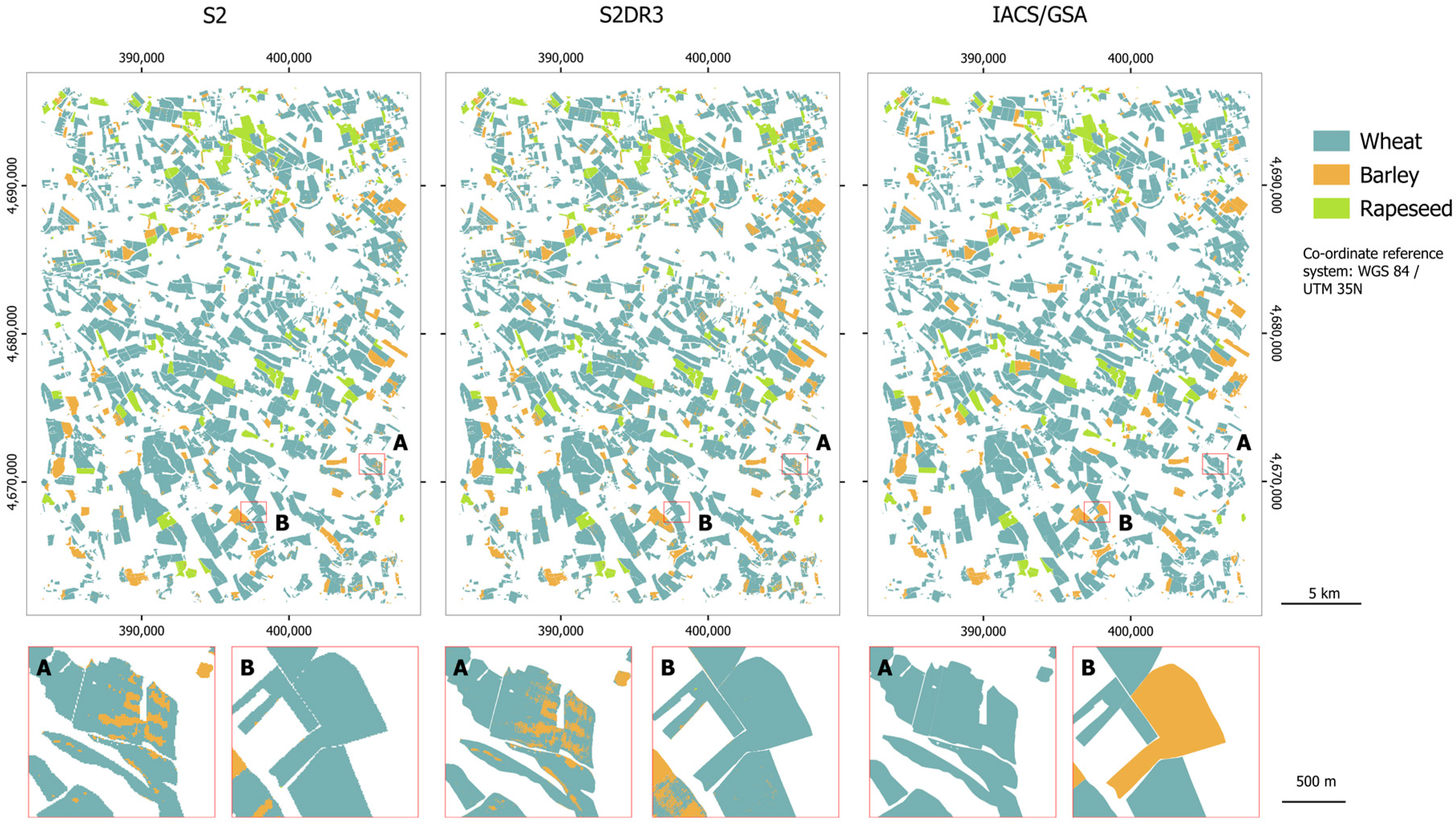
3.2. Crop Classification

The optimal combination of RF and SVC parameter values was different for each fold and also for S2DR3 and S2. No specific patterns were observed except that the number of trees was 100 or 200 in all cases except one, where it was 500. The best values for the other three RF parameters varied across all candidate values. This was also the case for the SVC parameters. In a preliminary experiment, we performed RF classifications with default parameters (except the number of trees, which was set to 500 based on recommendations in the literature [50]). The mean accuracies differed from those obtained with optimised parameters negligibly, mostly between 0% and 2%, except for the Producer’s accuracy of barley with S2, where the difference was 5% in favour of the classification with optimised parameters.
The outputs from the five classification iterations, covering different parts of Site 2, were combined to obtain a single map of winter crops in the site. We first visually examined the classification results using SVC as an example. The SVC maps for S2 and S2DR3 are shown in Figure 5, along with the reference data from IACS/GSA [32]. Both classifications represented well the general pattern of wheat dominating over the other two crops. At closer examination, two error patterns that were not sharply distinguished could be noticed. The first type was characterised by groups of wrongly classified pixels within a single field, which were more or less dispersed or formed strips (indicated with “A” in Figure 5). This noisy pattern is expected for pixel-based classification. The proportion of the field area which was wrongly classified varied significantly from case to case. The pattern of this type of error suggests that it is related to inhomogeneities in crop development or coverage within a field. The second error pattern included cases where almost all pixels in a field were consistently assigned to a wrong class without any significant noise within the field (indicated with “B” in Figure 5). They are therefore not associated with within-field inhomogeneities. The rapeseed appeared less affected by the errors compared to wheat and barley. The errors coincided spatially between S2 and S2DR3 to a greater extent. Hence, the two classifications were very similar. To quantitatively evaluate the similarity, the S2DR3 classification was aggregated to 10 m resolution using a mode (majority) rule and compared with the S2 classification, showing that over 96% of the pixels had the same class in both classifications at this spatial scale. More of the differences were spatially concentrated in particular fields. The agreement between the S2 and S2DR3 classifications further manifested in the very close values of the accuracy statistics (Table 4). The class-level statistics showed the good performance of both S2 and S2DR3 with respect to wheat and rapeseed. However, both image types failed with barley, which had low User’s and Producer’s accuracies. The class with which barley was most confused was wheat. Barley also showed greater variation in accuracy across the five cross-validation runs. The differences between the accuracies of the RF and SVC classifications were not notable, except for the User’s accuracy of barley, which was higher for SVC.

4. Discussion

4.1. Winter Crop Discrimination

The three winter crops have roughly the same growing period, spanning from October to July of the subsequent year, which makes them hard to distinguish based on their general growth pattern. Previous studies have demonstrated that successful crop identification is possible with multitemporal satellite imagery selected to include the key development stages of crops present in a specific study area [51]. Here, four S2DR3 images were available, one of which was too cloudy to be used for crop classification. Our dataset may not be optimal for winter crop discrimination as it is based on availability instead of careful consideration of crop calendars. Nevertheless, the results for rapeseed were very good, possibly because of the inclusion of the 30 April image, which corresponded to the flowering period of that crop. Figure 6 shows that the spectral profile of rapeseed differs from that of the other two crops, most notably on 30 April. The profiles of wheat and barley were very similar for all of the dates. Therefore, most classification errors were due to the misclassification of wheat and barley.
Discrimination between wheat and barley, which are from the same family, has been a subject of research for a long time [52]. Field experiments in [53] in Greece have found that spectral reflectance in the range 500–850 nm is very similar for wheat and barley throughout the season, arguably due to their similar canopy geometry. The authors recommended using more bands to increase the chances of the detection and identification of winter crops. The authors of [54] emphasised the importance of vegetation indices as a method to address the high spectral similarity of classes. Such indices should select the most significant parts of the reflectance spectrum characteristic of a particular crop. For instance, the index showing the best separability of wheat and barley in [54] was the red edge band of the RapidEye satellite. In addition, the study was conducted in a central European test site where winter barley phenological development was generally 10–20 days ahead of winter wheat, which potentially improves separability between these crops. The authors suggest that an acquisition date on which at least one of the crops has already reached the phenological stage of heading would be best suited for their separation. The study in [55] presented promising results for detecting the phenological development of winter wheat and winter barley using a time series of Sentinel-1 and S2. While not dealing with the discrimination of the two crops explicitly, such studies show that remote sensing instruments are sensitive to their phenology. Taking advantage of this sensitivity, the authors of Ref. [56] proposed a phenology-based method to discriminate barley from wheat based on S2 time series data. It was based on a new spectral–temporal feature enabling the automatic identification of the barley heading date. Ref. [57] utilised the difference in the NDVI during a period when barley is in the hard dough phenological stage while wheat is still not. With a decision tree-like algorithm based on the NDVI, Ref. [58] distinguished irrigated wheat and rain-fed barley in Lebanon. Ref. [59] demonstrated the ability to classify wheat and barley fields using a time series of Synthetic Aperture Radar (SAR) data from Sentinel-1 and a long short-term memory neural network. Other studies suggest that improved discrimination between wheat and barley is achieved by combining SAR and optical images [60].
In this study, the focus was more on the relative performance of S2DR3 compared with standard S2 images rather than on the best possible approach to mapping winter wheat and winter barley. Our test site is in a southerly location and has a shorter growing period of winter wheat and winter barley compared with that of published research from Central Europe. Further studies are needed under these conditions using dense image time series similar to [54] to explore optimal time periods to separate wheat and barley. The heading phenological stage occurs in May, which is usually very cloudy, and SAR data may be crucial for successful discrimination between wheat and barley.

4.2. The Performance of S2DR3

The virtually identical classification accuracy for both image types indicates that despite the data upscaling algorithm, S2DR3 retains the same level of spectral separation between classes as the original S2 data. Therefore, the improved spatial resolution does not come at the expense of degraded spectral quality. This was confirmed with both classification methods, RF and SVC. Nevertheless, the results presented here are based on a single dataset (location and season) and only three crop types, and the consistency of the above-mentioned conclusion will need to be further examined by other case studies. However, it is certain that the potential of S2DR3 for crop classification is promising.

5. Conclusions

With respect to the application of satellite data from S2DR3 to generate VIs for monitoring yields of organic barley in phase BBCH-41, the data presented are almost identical to the data from S2, but it should be noted that the number of VIs generated from S2 data that are positively correlated with yield is 12, and for VIs generated from S2DR3 data, the number is 11, as the latter NDVIG has low correlation with yield (r = −0.35); therefore, it is not recommended that this index be used in this phase and generated according to data from S2DR3. The S2DR3 data consistently showed stronger alignment with ground-truth yield metrics, particularly in phenologically critical phases like BBCH-41. Random Forest and SVC classifications confirmed that S2DR3 retained spectral fidelity despite its enhanced spatial resolution, ensuring the NDWI’s reliability at 1 × 1 m. Organic systems often exhibit higher spatial variability in soil moisture, organic matter, and vegetation cover due to limited synthetic inputs and reliance on natural soil processes. At 10 × 10 m resolution (S2), mixed pixels likely conflate soil and vegetation signals, particularly during early growth stages (e.g., BBCH-41) when soil exposure is significant. This blending may explain the NDWI’s negative correlation with yield at this scale, as soil moisture (high NDWI) is inversely related to crop biomass. In contrast, 1 × 1 m resolution (S2DR3) mitigates mixed-pixel effects, isolating plant-specific water content and aligning the NDWI positively with yield. In the BBCH-51 phase, it was determined more appropriate to use the S2DR3 data, since all but one of the VIs tested showed a strong or very high correlation with the yield of organic barley. In phase BBCH-77, the data from S2DR3 are more suitable for predicting yields compared to S2. The vegetation indices generated in this phase from data from the S2 satellite are unsuitable for determining and predicting the yields of biological barley, as only VI NDRE2 (r = 0.37) has an average positive correlation. To confirm the application of S2DR3 data to organic barley yield monitoring, it is necessary to test the data in other phenological phases. The enhanced performance of specific vegetation indices (VIs) with Sentinel-2 Deep Resolution 3.0 (S2DR3) can be attributed primarily to its superior spatial resolution (1 × 1 m versus 10 × 10 m), which fundamentally alters spectral–biophysical relationships in organic farming systems. This resolution advantage enables S2DR3 to better capture the inherent spatial heterogeneity in organically managed fields, where crop development, soil exposure, and weed pressure vary significantly at sub-field scales. The dramatic reversal in NDWI’s correlation pattern—from strongly negative with S2 (r = −0.80) to strongly positive with S2DR3 (r = 0.66)—demonstrates how mixed-pixel effects at coarser resolutions can confound the relationship between spectral indices and crop conditions. Indices like the TCARI, TO, and NDRE1, which showed consistent reliability across phenological stages with S2DR3, likely benefit from reduced soil background interference and enhanced sensitivity to subtle variations in chlorophyll content, canopy structure, and water status. Additionally, the red edge-based indices (NDRE1, NDRE2) performed substantially differently at varying resolutions, suggesting that the transition bands between visible and near-infrared regions capture critical information about crop physiology that is resolution-dependent and particularly valuable in organic systems where synthetic inputs are limited and natural spatial variability is pronounced.
Concerning the classification of winter crops, S2 and S2DR3 performed equally well, and this was observed with both classification methods, RF and SVC.

Author Contributions

Conceptualisation, L.F. and M.C.; methodology, L.F., M.C., I.K. and P.D.; validation, I.K. and P.D.; resources, L.F.; data curation, L.F., M.C., P.D. and I.K.; writing—original draft preparation, M.C. and L.F.; writing—review and editing, I.K. and P.D.; visualisation, M.C., I.K. and P.D.; supervision, L.F.; funding acquisition, L.F. and M.C. All authors have read and agreed to the published version of the manuscript.

Funding

This worked received no funding.

Data Availability Statement

The S2DR3 data can be accessed upon written request to DigiFarm (Norway). The crop yield data are collected within the National Research Programme “Young scientists and postdoctoral students—2” approved by DCM 206/07.04.2022 and are available at the authors’ discretion following the programme’s data citation guidelines for reuse.

Acknowledgments

The authors thank DigiFarm (Norway) and personally thank Aaron Smith for providing the S2DR3 data for this experiment. We thank the organic certification company Balkan Biocert (Bulgaria) for putting us in touch with an organically certified farmer. We also thank the organically certified farmer ET “Borislav Slavchev” from the village of Byala Reka, Plovdiv region, central-southern Bulgaria, for providing access to his farm. The State Fund “Agriculture” provided the IACS/GSA data. The S2DR3 data were preprocessed by Nevena Miteva, of whom the authors are appreciative. This work was partially supported by the Bulgarian Ministry of Education and Science under the National Research Programme “Young scientists and postdoctoral students—2” approved by DCM 206/07.04.2022. Dessislava Ganeva, English language editor at the journal Aerospace Research of Bulgaria (ISSN 1313-0927), checked the revised manuscript for English language use. The authors are acknowledged to Bulgarian Ministry of Education and Science which supported the field data collection under the National Research Programme “Young scientists and postdoctoral students—2” approved by DCM 206/07.04.2022 to which Milen Chanev is beneficiary.

Conflicts of Interest

The authors declare no conflicts of interest. The funders had no role in the study’s design; in the collection, analyses, or interpretation of data; in the writing of the manuscript; or in the decision to publish the results.

Abbreviations

The following abbreviations are used in this manuscript:
Biologische Bundesanstalt, Bundessortenamt und CHemische Industrie
(Phenological Scale)
BBCH
Canopy Chlorophyll Content IndexCCCI
Common Agricultural PolicyCAP
Deep ResolutionDR
Difference Vegetation IndexDVI
EOS Data AnalyticsEOSDA
Enhanced Vegetation IndexEVI
Two-band Enhanced Vegetation IndexEVI2
Green Chlorophyll Vegetation IndexGCVI
Geographic Information SystemGIS
Geospatial ApplicationGSA
Integrated Administration and Control SystemIACS
Multidisciplinary Digital Publishing InstituteMDPI
Normalised Difference Red Edge Index 1NDRE1
Normalised Difference Red Edge Index 2NDRE2
Normalised Difference Vegetation IndexNDVI
Green Normalised Difference Vegetation IndexNDVIG
Normalised Difference Water IndexNDWI
Normalised Multi-band Drought IndexNMDI
Optimised Soil-Adjusted Vegetation IndexOSAVI
Quantum Geographic Information SystemQGIS
Random ForestRF
Sentinel-2S2
Sentinel-2 Deep Resolution 3.0S2DR3
Single-Image Super-ResolutionSISR
Simple RatioSR
Triangular Optical ReflectanceTO
Vegetation IndexVI

References

  1. Leitner, C.; Vogl, C.H. Farmers’ Perceptions of the Organic Control and Certification Process in Tyrol, Austria. Sustainability 2020, 12, 9160. [Google Scholar] [CrossRef]
  2. Novikova, A.; Rocchi, L.; Startiene, G. Integrated Assessment of Farming System Outputs: Lithuanian Case Study. Inžinerinė Ekon. 2020, 31, 282–290. [Google Scholar] [CrossRef]
  3. Novikova, A.; Zemaitiene, R.; Marks-Bielska, R.; Bielski, S. Assessment of the Environmental Public Goods of the Organic Farming System: A Lithuanian Case Study. Agriculture 2024, 14, 362. [Google Scholar] [CrossRef]
  4. Aleksiev, G. Sustainable Development of Bulgarian Organic Agriculture. Trakia J. Sci. 2020, 18, 603–606. [Google Scholar] [CrossRef]
  5. Georgieva, N.; Kosev, V.; Vasileva, I. Suitability of Lupinus albus L. Genotypes for Organic Farming in Central Northern Bulgaria. Agronomy 2024, 14, 506. [Google Scholar] [CrossRef]
  6. Lone, A.H.; Rashid, I. Sustainability of Organic Farming: A Review via Three Pillar Approach. Sustain. Agri Food Environ. Res. Discontin. 2023, 11, 1–24. [Google Scholar] [CrossRef]
  7. Rozaki, Z.; Yudanto, R.S.B.; Triyono; Rahmawati, N.; Alifah, S.; Ardila, R.A.; Pamungkas, H.W.; Fathurrohman, Y.E.; Man, N. Assessing the sustainability of organic rice farming in Central Java and Yogyakarta: An economic, ecological, and social evaluation. Org. Farming 2024, 10, 142–158. [Google Scholar] [CrossRef]
  8. Kociszewski, K.; Graczyk, A.; Mazurek-Łopacinska, K.; Sobocińska, M. Social Values in Stimulating Organic Production Involvement in Farming—The Case of Poland. Sustainability 2020, 12, 5945. [Google Scholar] [CrossRef]
  9. Gitelson, A.A. Remote Sensing Estimation of Crop Biophysical Characteristics at Various Scales. Hyperspectral Remote Sens. Veget. 2016, 20, 329. [Google Scholar]
  10. Atanasova, D.; Bozhanova, V.; Biserkov, V.; Maneva, V. Distinguishing Areas of Organic, Biodynamic and Conventional Farming by Means of Multispectral Images—A Pilot Study. Biotechnol. Biotechnol. Equip. 2021, 35, 977–993. [Google Scholar] [CrossRef]
  11. Li, G.; Wan, S.; Zhou, J.; Yang, Z.; Qin, P. Leaf Chlorophyll Fluorescence, Hyperspectral Reflectance, Pigments Content, Malondialdehyde and Proline Accumulation Responses of Castor Bean (Ricinus communis L.) Seedlings to Salt Stress Levels. Ind. Crops Prod. 2010, 31, 13–19. [Google Scholar] [CrossRef]
  12. Usha, K.; Singh, B. Potential Applications of Remote Sensing in Horticulture—A Review. Sci. Hortic. 2013, 153, 71–83. [Google Scholar] [CrossRef]
  13. Chanev, M.; Filchev, L.; Ivanova, D. Opportunities for Remote Sensing Applications in Organic Cultivation of Cereals—A Review. J. Bulg. Geogr. Soc. 2020, 43, 31–36. [Google Scholar] [CrossRef]
  14. Nadzirah, R.; Qurrohman, T.; Indarto, I.; Putra, B.T.W.; Andriyani, I. Estimating Harvest Yield Using Sentinel-2 Derivative Vegetation Indices (Case Study: Organic Paddy in Candipuro, Lumajang). In AIP Conference Proceedings; AIP Publishing: Melville, NY, USA, 2024; Volume 3176. [Google Scholar] [CrossRef]
  15. Tarasiewicz, T.; Nalepa, J.; Farrugia, R.A.; Valentino, G.; Chen, M.; Briffa, J.A.; Kawulok, M. Multitemporal and multispectral data fusion for super-resolution of Sentinel-2 images. IEEE Trans. Geosci. Remote Sens. 2023, 61, 1–19. [Google Scholar] [CrossRef]
  16. Jumaah, H.J.; Rashid, A.A.; Saleh, S.A.R.; Jumaah, S.J. Deep neural remote sensing and Sentinel-2 satellite image processing of Kirkuk City, Iraq for sustainable prospective. J. Opt. Photonics Res. 2024, 1–9. [Google Scholar] [CrossRef]
  17. Michel, J.; Vinasco-Salinas, J.; Inglada, J.; Hagolle, O. SEN2VENµS, a Dataset for the Training of Sentinel-2 Super-Resolution Algorithms. Data 2022, 7, 96. [Google Scholar] [CrossRef]
  18. Weiss, M.; Jacob, F.; Duveiller, G. Remote sensing for agricultural applications: A meta-review. Remote Sens. Environ. 2020, 236, 111402. [Google Scholar] [CrossRef]
  19. Akhtman, Y. Sentinel-2 Deep Resolution. Available online: https://medium.com/@ya_71389/sentinel-2-deep-resolution-3-0-c71a601a2253 (accessed on 23 January 2024).
  20. Kawulok, M.; Kawulok, J.; Smolka, B.; Celebi, M.E. (Eds.) Super-Resolution for Remote Sensing; Springer Cham: Cham, Switzerland, 2024; 384p. [Google Scholar] [CrossRef]
  21. Ye, S.; Zhao, S.; Hu, Y.; Xie, C. Single-Image Super-Resolution Challenges: A Brief Review. Electronics 2023, 12, 2975. [Google Scholar] [CrossRef]
  22. Dixit, M.; Yadav, R.N. A Review of Single Image Super Resolution Techniques using Convolutional Neural Networks. Multimed Tools Appl. 2024, 83, 29741–29775. [Google Scholar] [CrossRef]
  23. Al-Mekhlafi, H.; Liu, S. Single image super-resolution: A comprehensive review and recent insight. Front. Comput. Sci. 2024, 18, 181702. [Google Scholar] [CrossRef]
  24. Wang, P.; Bayram, B.; Sertel, E. A comprehensive review on deep learning based remote sensing image super-resolution methods. Earth-Sci. Rev. 2022, 232, 104110. [Google Scholar] [CrossRef]
  25. Lei, S.; Shi, Z.; Zou, Z. Super-Resolution for Remote Sensing Images via Local–Global Combined Network. IEEE Geosci. Remote Sens. Lett. 2017, 14, 1243–1247. [Google Scholar] [CrossRef]
  26. Ninov, N. Chapter 4: Soils. In Geography of Bulgaria; Kopralev, I., Yordanova, M., Mladenov, C., Eds.; ForCom: Sofia, Bulgaria, 2002; pp. 277–315. (In Bulgarian) [Google Scholar]
  27. Shishkov, T.; Kolev, N. The Soils of Bulgaria; Springer: Cham, Switzerland, 2014; 208p. [Google Scholar]
  28. Kopralev, I.; Yordanova, M.; Mladenov, C. (Eds.) Geography of Bulgaria; ForCom: Sofia, Bulgaria, 2002; 760p. (In Bulgarian) [Google Scholar]
  29. Marinkov, E.; Dimova, D. Opitno Delo i Biometriya; Akademichno Izdatelstvo na VSI: Plovdiv, Bulgaria, 1999; 262p. (In Bulgarian) [Google Scholar]
  30. Meier, U. Growth Stages of Mono- and Dicotyledonous Plants: BBCH Monograph; Open Agrar Repositorium: Quedlinburg, Germany, 2018. [Google Scholar] [CrossRef]
  31. Shanin, J. Metodika na Polskija Opit; Izdatelstvo na BAN: Sofia, Bulgaria, 1977; 383p. (In Bulgarian) [Google Scholar]
  32. Integrated Administration and Control System (IACS). Available online: https://agriculture.ec.europa.eu/common-agricultural-policy/financing-cap/assurance-and-audit/managing-payments_en (accessed on 24 January 2024).
  33. Rouse, J.W.; Haas, R.H.; Schell, J.A.; Deering, D.W. Monitoring the Vernal Advancement and Retrogradation (Green Wave Effect) of Natural Vegetation. NASA Technical Reports Server (NTRS), USA, NASA-CR-132982. 1973. Available online: https://ntrs.nasa.gov/api/citations/19730017588/downloads/19730017588.pdf (accessed on 24 January 2024).
  34. Metternicht, G. Vegetation Indices Derived from High-Resolution Airborne Videography for Precision Crop Management. Int. J. Remote Sens. 2003, 24, 2855–2877. [Google Scholar] [CrossRef]
  35. Gao, B.C. Normalized Difference Water Index for Remote Sensing of Vegetation Liquid Water from Space. Imaging Spectrom. 1995, 2480, 225–236. [Google Scholar]
  36. Wang, L.; Qu, J.J. NMDI: A Normalized Multi-Band Drought Index for Monitoring Soil and Vegetation Moisture with Satellite Remote Sensing. Geophys. Res. Lett. 2007, 34, L20405. [Google Scholar] [CrossRef]
  37. Rondeaux, G.; Steven, M.; Baret, F. Optimization of Soil-Adjusted Vegetation Indices. Remote Sens. Environ. 1996, 55, 95–107. [Google Scholar] [CrossRef]
  38. Jordan, C.F. Derivation of Leaf-Area Index from Quality of Light on the Forest Floor. Ecology 1969, 50, 663–666. [Google Scholar] [CrossRef]
  39. Steven, M.D. The Sensitivity of the OSAVI Vegetation Index to Observational Parameters. Remote Sens. Environ. 1998, 63, 49–60. [Google Scholar] [CrossRef]
  40. Huete, A.; Didan, K.; Miura, T.; Rodriguez, E.P.; Gao, X.; Ferreira, L.G. Overview of the Radiometric and Biophysical Performance of the MODIS Vegetation Indices. Remote Sens. Environ. 2002, 83, 195–213. [Google Scholar] [CrossRef]
  41. Daughtry, C.S.; Walthall, C.L.; Kim, M.S.; De Colstoun, E.B.; McMurtrey, J.E., III. Estimating Corn Leaf Chlorophyll Concentration from Leaf and Canopy Reflectance. Remote Sens. Environ. 2000, 74, 229–239. [Google Scholar] [CrossRef]
  42. Haboudane, D.; Miller, J.R.; Tremblay, N.; Zarco-Tejada, P.J.; Dextraze, L. Integrated Narrow-Band Vegetation Indices for Prediction of Crop Chlorophyll Content for Application to Precision Agriculture. Remote Sens. Environ. 2002, 81, 416–426. [Google Scholar] [CrossRef]
  43. Gitelson, A.A.; Gritz, Y.; Merzlyak, M.N. Relationships Between Leaf Chlorophyll Content and Spectral Reflectance and Algorithms for Non-Destructive Chlorophyll Assessment in Higher Plant Leaves. J. Plant Physiol. 2003, 160, 271–282. [Google Scholar] [CrossRef]
  44. Gitelson, A.; Merzlyak, M.N. Spectral Reflectance Changes Associated with Autumn Senescence of Aesculus hippocastanum L. and Acer platanoides L. Leaves. Spectral Features and Relation to Chlorophyll Estimation. J. Plant Physiol. 1994, 143, 286–292. [Google Scholar] [CrossRef]
  45. Barnes, E.M.; Clarke, T.R.; Richards, S.E.; Colaizzi, P.D.; Haberland, J.; Kostrzewski, M.; Waller, P.; Choi, C.; Riley, E.; Thompson, T.; et al. Coincident Detection of Crop Water Stress, Nitrogen Status and Canopy Density Using Ground Based Multispectral Data. In Proceedings of the Fifth International Conference on Precision Agriculture, Bloomington, MN, USA, 16–19 July 2000; Volume 1619. [Google Scholar]
  46. Breiman, L. Random Forests. Mach. Learn. 2001, 45, 5–32. [Google Scholar] [CrossRef]
  47. Drusch, M.; Del Bello, U.; Carlier, S.; Colin, O.; Fernandez, V.; Gascon, F.; Hoersch, B.; Isola, C.; Laberinti, P.; Martimort, P. Sentinel-2: ESA’s Optical High-Resolution Mission for GMES Operational Services. Remote Sens. Environ. 2012, 120, 25–36. [Google Scholar] [CrossRef]
  48. Vapnik, V.N. The Nature of Statistical Learning Theory. Nat. Stat. Learn. Theory 1995, 38, 409. [Google Scholar]
  49. Pedregosa, F.; Varoquaux, G.; Gramfort, A.; Michel, V.; Thirion, B.; Grisel, O.; Blondel, M.; Prettenhofer, P.; Weiss, R.; Dubourg, V.; et al. Scikit-learn: Machine Learning in Python. J. Mach. Learn. Res. 2011, 12, 2825–2830. [Google Scholar]
  50. Belgiu, M.; Drăguţ, L. Random forest in remote sensing: A review of applications and future directions. ISPRS J. Photogrammetry Remote Sens. 2016, 114, 24–31. [Google Scholar] [CrossRef]
  51. Peña-Barragán, J.M.; Ngugi, M.K.; Plant, R.E.; Six, J. Object-based crop identification using multiple vegetation indices, textural features and crop phenology. Remote Sens. Environ. 2011, 115, 1301–1316. [Google Scholar] [CrossRef]
  52. Peştemalci, V.; Dinç, U.; Yeğingil, I.; Kandirmaz, M.; Çullu, M.A.; Öztürk, N.; Aksoy, E. Acreage estimation of wheat and barley fields in the province of Adana, Turkey. Int. J. Remote Sens. 1995, 16, 1075–1085. [Google Scholar] [CrossRef]
  53. Toulios, L.; Tournaviti, A. Cereals discrimination based on spectral measurements. In Proceedings of the International Symposium on Remote Sensing, Crete, Greece, 23–27 September 2002. [Google Scholar] [CrossRef]
  54. Gerstmann, H.; Möller, M.; Gläßer, C. Optimization of spectral indices and long-term separability analysis for classification of cereal crops using multi-spectral RapidEye imagery. Int. J. Appl. Earth Obs. Geoinf. 2016, 52, 115–125. [Google Scholar] [CrossRef]
  55. Harfenmeister, K.; Itzerott, S.; Weltzien, C.; Spengler, D. Detecting Phenological Development of Winter Wheat and Winter Barley Using Time Series of Sentinel-1 and Sentinel-2. Remote Sens. 2021, 13, 5036. [Google Scholar] [CrossRef]
  56. Ashourloo, D.; Nematollahi, H.; Huete, A.; Aghighi, H.; Azadbakht, M.; Shahrabi, H.S.; Goodarzdashti, S. A new phenology-based method for mapping wheat and barley using time-series of Sentinel-2 images. Remote Sens. Environ. 2022, 280, 113206. [Google Scholar] [CrossRef]
  57. Heupel, K.; Spengler, D.; Itzerott, S. A Progressive Crop-Type Classification Using Multitemporal Remote Sensing Data and Phenological Information. J. Photogramm. Remote Sens. Geoinf. Sci. 2018, 86, 53–69. [Google Scholar] [CrossRef]
  58. Nasrallah, A.; Baghdadi, N.; Mhawej, M.; Faour, G.; Darwish, T.; Belhouchette, H.; Darwich, S. A Novel Approach for Mapping Wheat Areas Using High Resolution Sentinel-2 Images. Sensors 2018, 18, 2089. [Google Scholar] [CrossRef]
  59. Pfeil, I.; Reuß, F.; Vreugdenhil, M.; Navacchi, C.; Wagner, W. Classification of Wheat And Barley Fields Using Sentinel-1 Backscatter. In Proceedings of the IEEE International Geoscience and Remote Sensing Symposium (IGARSS 2020), Waikoloa, HI, USA, 26 September–2 October 2020; pp. 140–143. [Google Scholar] [CrossRef]
  60. Marini, M.F. Discriminación de trigo y cebada empleando imágenes satelitales ópticas y radar: Estudio de caso: Partido de Coronel Rosales (Argentina). Investig. Geográficas 2021, 104, e60173. [Google Scholar] [CrossRef]
Figure 1. (A) The overall location of the study area in Bulgaria. The image data used in this study correspond to Sentinel-2 tile T35TLG shown as a red square. (B) Sentinel-2 Deep Resolution 3.0 imagery in natural colours from 30 April 2023 obtained over tile T35TLG. The red rectangle and dot indicate the location of the area used for crop classification and the field used for collecting crop yield data, respectively. Closer looks at these two sites are shown in (C,D), respectively. (E) Subsets of Sentinel-2 Deep Resolution 3.0 (top, 1 m spatial resolution) and Sentinel-2 (10 m spatial resolution) obtained over an arbitrary agricultural area (location shown with arrow on (C); 30 April 2023; natural colours).
Remotesensing 17 00957 g001
Figure 2. Correlation between yield of organic barley from S2DR3 data (blue) and S2 data (orange) in phase BBCH-41.
Remotesensing 17 00957 g002
Figure 3. Correlation between yield of organic barley from S2DR3 data (blue) and S2 data (orange) in phase BBCH-51.
Remotesensing 17 00957 g003
Figure 4. Correlation between yield of organic barley from S2DR3 data (blue) and S2 data (orange) in phase BBCH-77.
Remotesensing 17 00957 g004
Figure 5. Maps showing the distribution of the three winter crops according to the SVC classifications of the Sentinel-2 (S2; left) and Sentinel-2 Deep Resolution 3.0 (S2DR3; middle) multitemporal datasets and the reference vector data (IACS/GSA; right). The areas indicated with “A” and “B” illustrate two typical error patterns (see text for more details). The maps cover Site 2 (see Figure 1C for its location).
Remotesensing 17 00957 g005
Figure 6. Spectral profiles of the three winter crops for the two image types, S2DR3 and S2, and the three dates. Dots represent the mean and error bars represent the standard deviation of 50 randomly selected pixels for each crop. Pixels were sampled at image native resolution, i.e., 1 m for S2DR3 and 10 m/20 m for S2. Sampling locations were the same for S2DR3 and S2.
Remotesensing 17 00957 g006
Table 1. Dates of the satellite images (S2 and S2DR3), cloud coverage (% of the tile’s area), and usage in this study.
UsageClouds (%)Image Date
Crop classification136 March 2023
Yield3715 April 2023
Yield/Crop classification4030 April 2023
Yield/Crop classification29 June 2023
Table 2. Vegetation index formula.
ReferenceFormulaVegetation Index
[33](B8 − B4)/(B8 + B4)NDVI
[34](B6 − B3)/(B3 + B6)NDVIG
[35](B8 − B12)/(B8 + B12)NDWI
[36](B8a − (B11 − B12))/(B8a + (B11 + B12))NMDI
[37](B8 − B4)/(B8 + B4 + 0.16)OSAVI
[38]B8/B4SR
[39]B8 − B4DVI
[40]2.5 × (B8 − B4)/(B8 + 6 × B4 − 7.5 × B2 + 1)EVI
[41]2.5 × (B8 − B4)/(B8 + 2.4 × B4 + 1)EVI2
[42]TCARI/OSAVITO
[43]B8 − B3GDVI
[43]B8/B3 − 1GCVI
[44](B6 − B5)/(B6 + B5)NDRE1
[44](B7 − B5)/(B7 + B5)NDRE2
[45]NDRE1/OSAVICCCI
Table 3. The parameters of the Random Forest (RF) and Support Vector Classification (SVC) classifiers were optimised in this study.
Default Value in EnMAP-Box v3.15Candidate ValuesDescription [49]Parameter [49]Classifier
100100, 200, 300, 400, 500, 600, 700, 800, 900, 1000The number of trees in the forestn_estimatorsRF
Square root of the number of features3, 4, 5, 6, 7The number of features to consider when looking for the best splitmax_features
22, 3, 5, 10, 15, 20, 30The minimum number of samples required to split an internal nodemin_samples_split
11, 2, 3, 4The minimum number of samples required to be at a leaf nodemin_samples_leaf
-0.00001, 0.0001, 0.001, 0.01, 0.1, 1, 10, 100Kernel coefficientgammaSVC
-0.01, 0.1, 1, 10, 100, 1000, 10,000, 100,000Regularisation parameterC
Table 4. Winter crop classification accuracy. Values represent the mean (minimum; maximum) of five-fold cross-validation.
Support Vector ClassificationRandom Forest
S2S2DR3S2S2DR3
Winter wheat
0.96 (0.94; 0.98)0.96 (0.94; 0.98)0.97 (0.95; 0.98)0.96 (0.95; 0.98)User’s accuracy
0.97 (0.95; 0.98)0.95 (0.87; 0.97)0.90 (0.87; 0.94)0.90 (0.85; 0.93)Producer’s accuracy
Winter barley
0.78 (0.69; 0.86)0.70 (0.49; 0.82)0.53 (0.34; 0.67)0.52 (0.35; 0.65)User’s accuracy
0.70 (0.59; 0.88)0.70 (0.59; 0.88)0.74 (0.65; 0.87)0.73 (0.63; 0.86)Producer’s accuracy
Winter rapeseed
0.95 (0.90; 0.99)0.95 (0.90; 0.98)0.93 (0.86; 0.95)0.91 (0.85; 0.95)User’s accuracy
0.98 (0.97; 0.99)0.98 (0.96; 0.99)0.99 (0.98; 1.00)0.99 (0.98; 0.99)Producer’s accuracy
Disclaimer/Publisher’s Note: The statements, opinions and data contained in all publications are solely those of the individual author(s) and contributor(s) and not of MDPI and/or the editor(s). MDPI and/or the editor(s) disclaim responsibility for any injury to people or property resulting from any ideas, methods, instructions or products referred to in the content.

