


Subsidence Monitoring in Emilia-Romagna Region (Italy) from 2016 to 2021: From InSAR and GNSS Integration to Data Analysis

 ,
,  ,
,  ,
,  ,
, 
Abstract
1. Introduction
1.1. The Subsidence Phenomenon and Monitoring Techniques
1.2. The Emilia-Romagna Region
1.3. Evolution of the Emilia-Romagna Subsidence Maps
1.4. The 2016–2021 Emilia-Romagna Subsidence Map
2. Materials and Methods
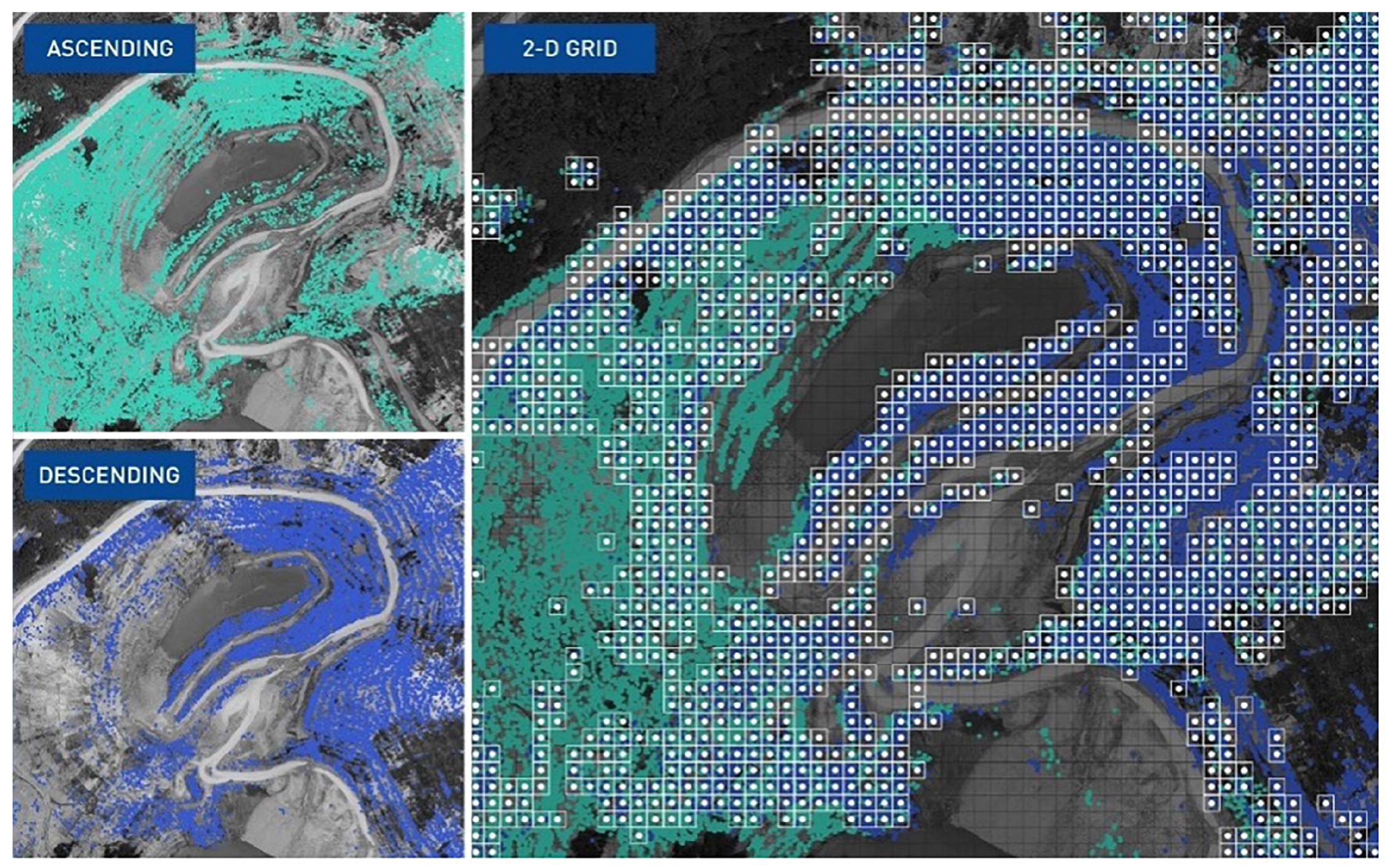
2.1. SAR Data and the SqueeSAR® Approach
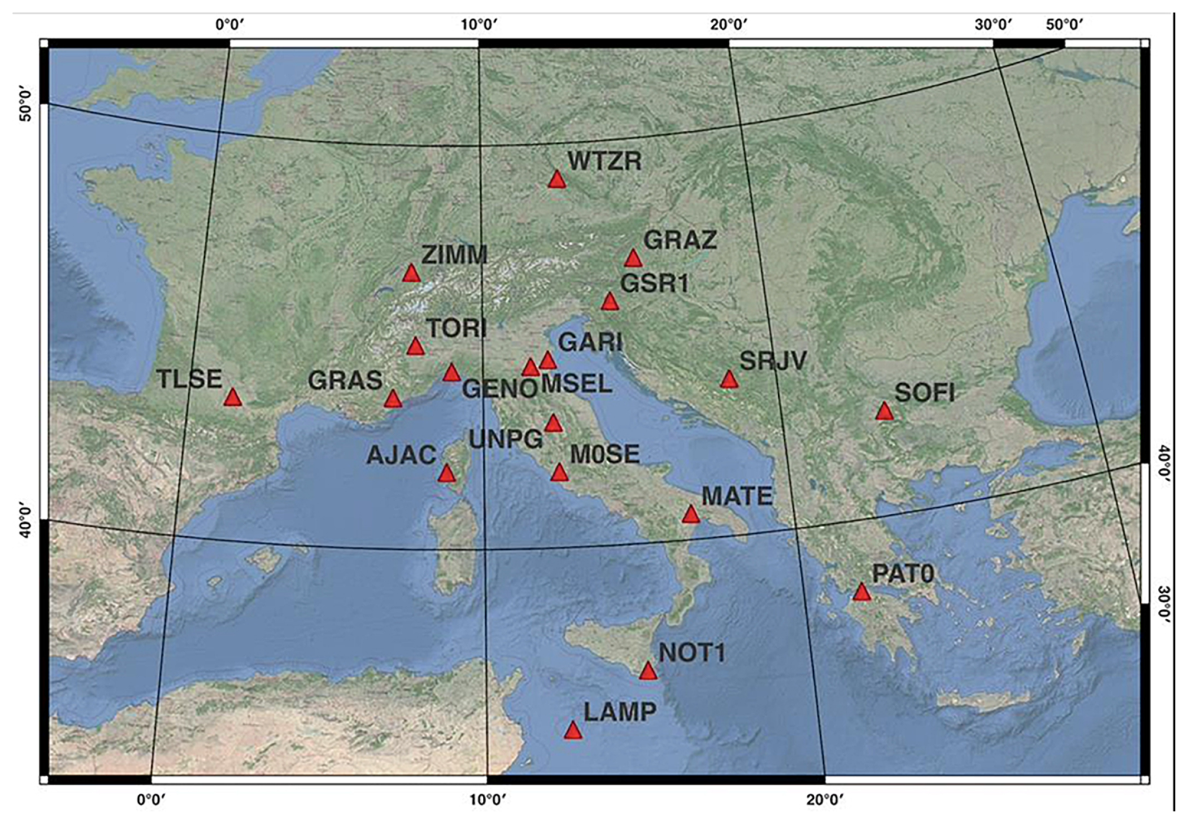
2.2. GNSS Data and the PPP Approach
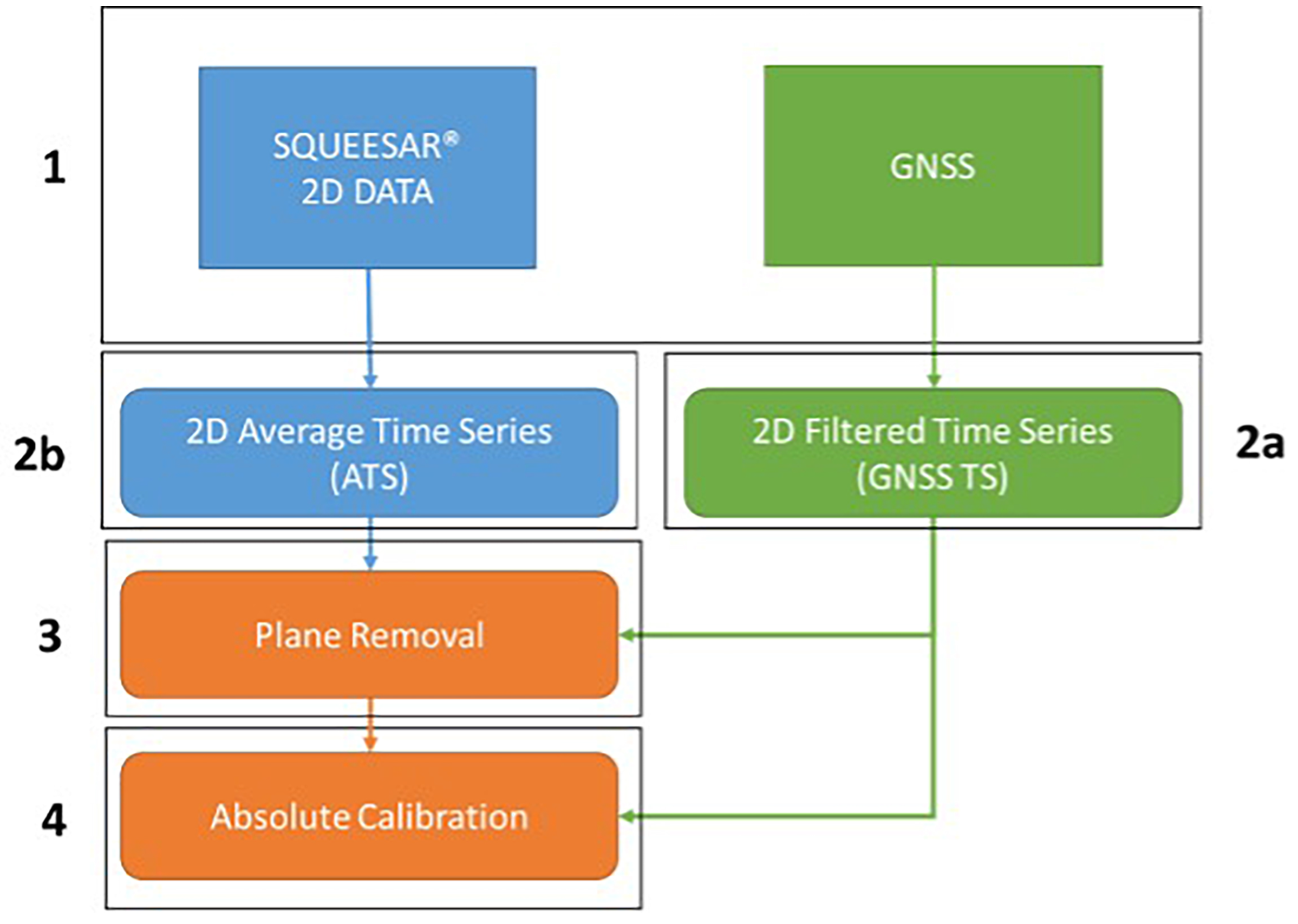
2.3. InSAR Calibration
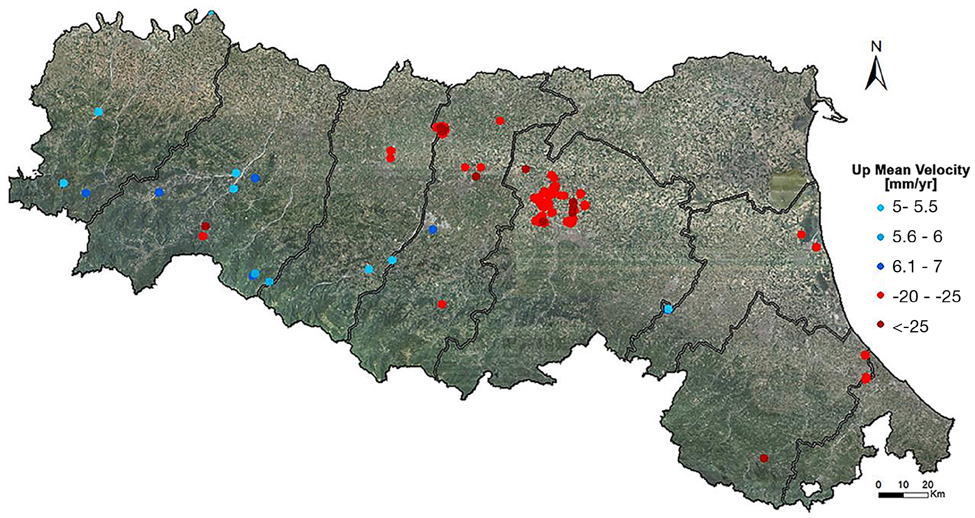
3. Results
- The mean velocities and the time series of the GNSS permanent stations, obtained from the precise point positioning approach;
- The LOS and east–up results of the SqueeSAR® interferometric analysis;
- The basic cartographic data and database of high-resolution satellite images.
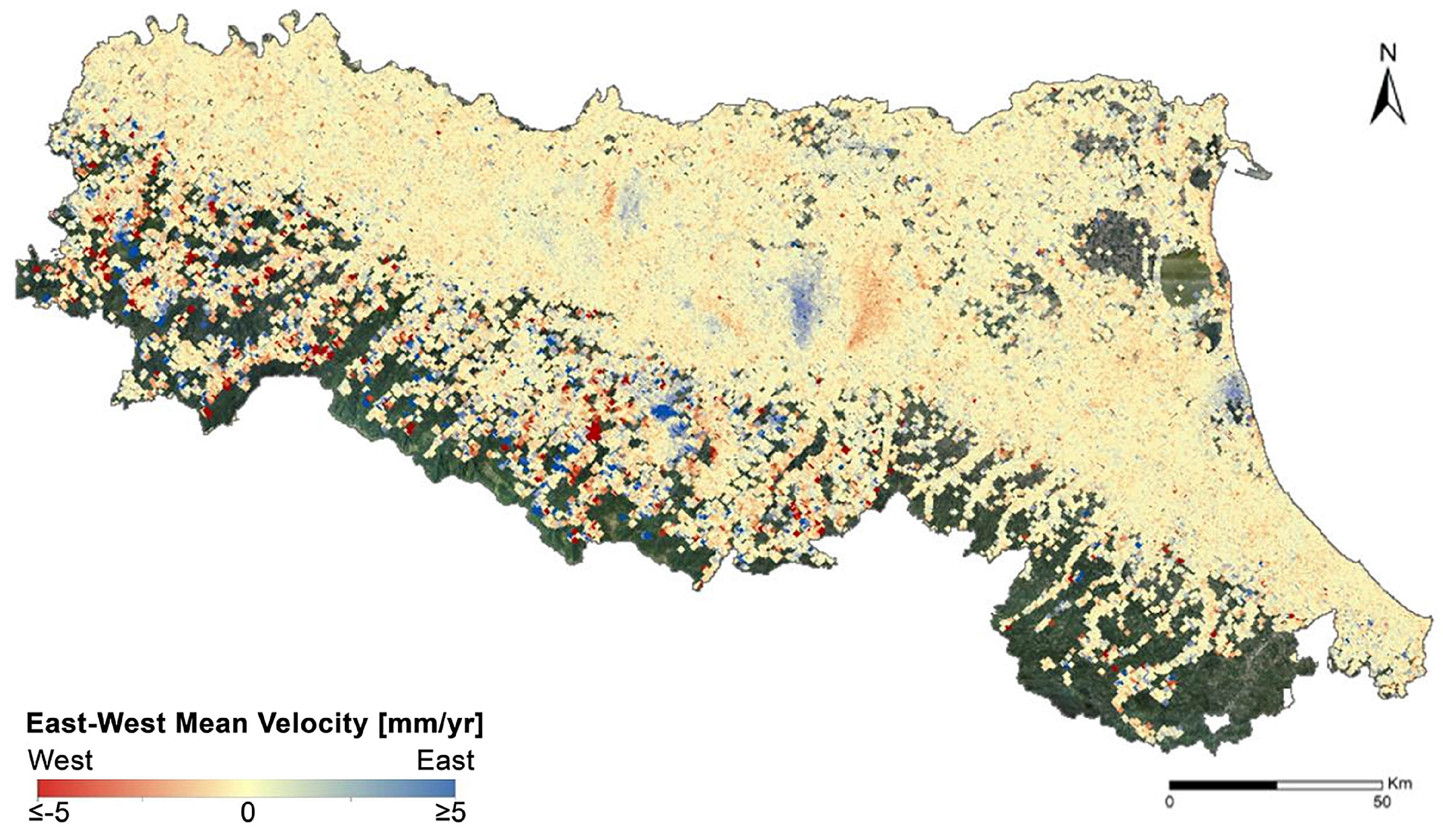
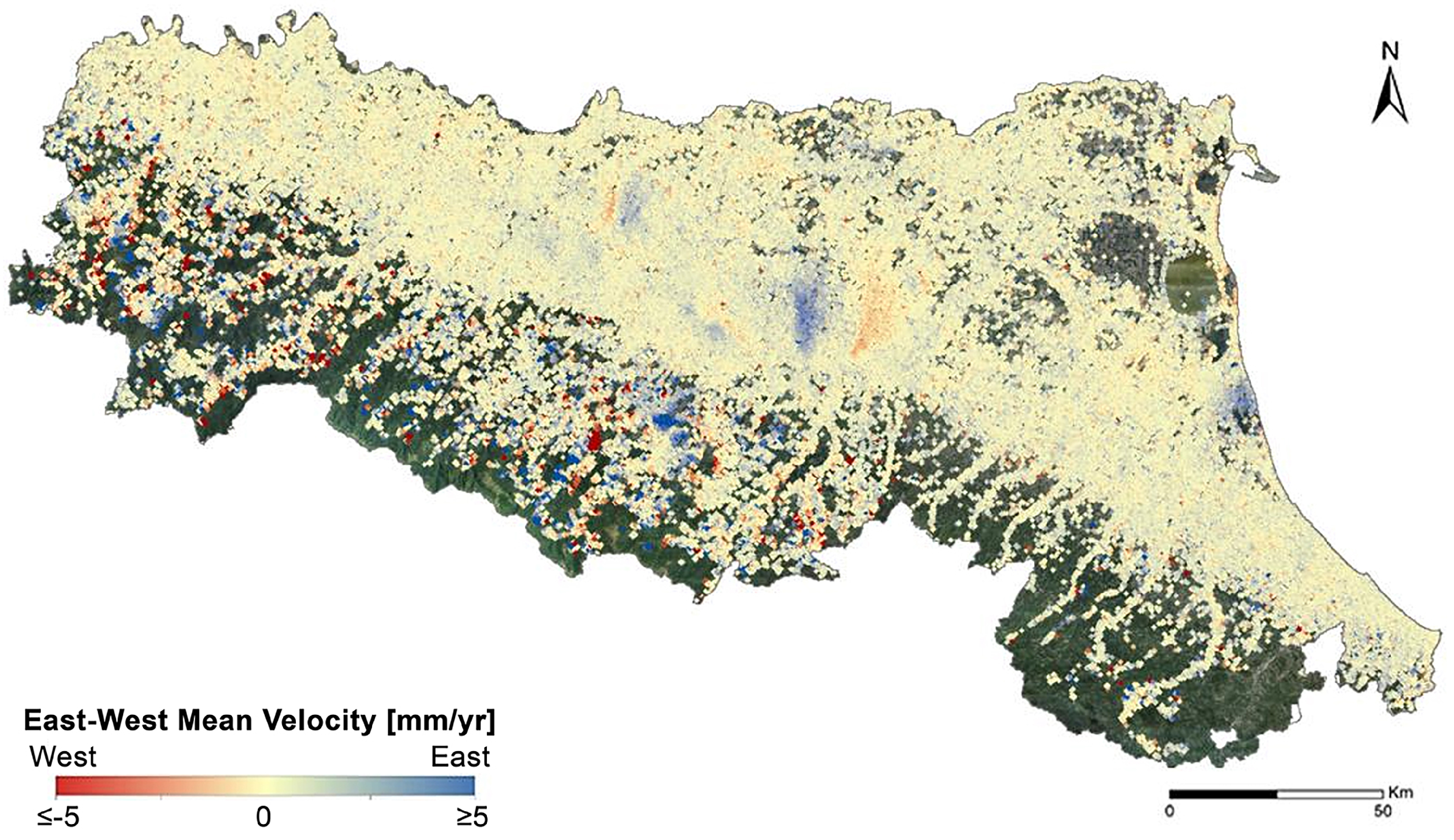
3.1. InSAR Measurement Points and East–West Components
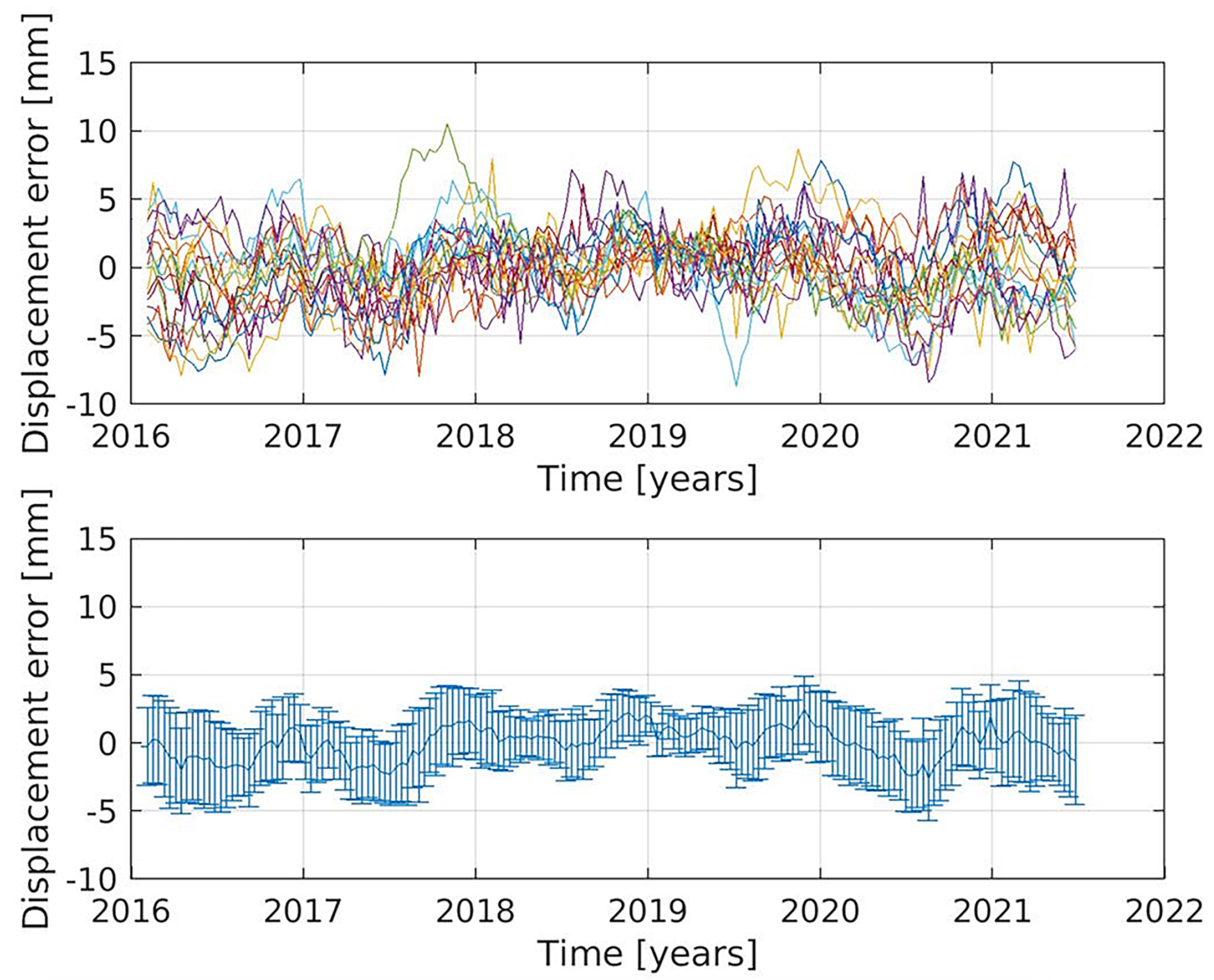
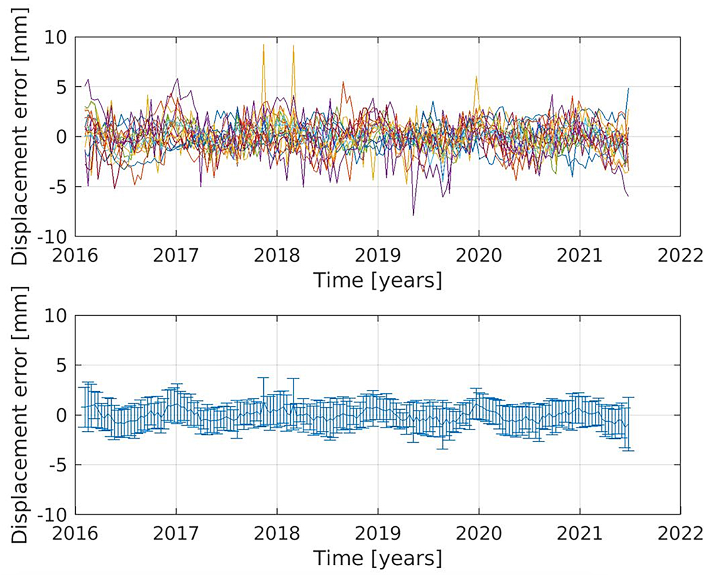
3.2. GNSS Mean Velocities and Time Series in ETRF
3.3. Calibration of SqueeSAR® Pseudo-MP

| Marker | GNSS [mm/yr] | SqueeSAR® [mm/yr] | [mm/yr] | GNSS [mm/yr] | SqueeSAR® [mm/yr] | [mm/yr] |
|---|---|---|---|---|---|---|
| BGDR | 0.9 | - | - | 0.2 | - | - |
| BLGN | −8.3 | −7.5 | 1 | −0.9 | −1.4 | −0.5 |
| BOBB | −0.6 | 0 | 0.6 | 0.3 | 0.5 | 0.2 |
| BRAS | 0.5 | −0.9 | −1.4 | 0 | 0.3 | 0.3 |
| BRIS | 0.6 | - | - | 1.1 | - | - |
| CAST | 0.8 | −0.6 | −1.4 | 0 | −0.1 | −0.1 |
| CODI | −2.8 | −3.1 | −0.3 | 0 | 0.1 | 0.1 |
| FERR | −1 | −2.4 | −1.4 | 0.4 | 0.4 | 0 |
| GARI | −2.8 | −2.9 | −0.1 | −0.3 | 0.1 | 0.4 |
| GUAS | −1.6 | −1.8 | −0.2 | 0.1 | 0.2 | 0.1 |
| ITIM | −0.4 | −1.3 | −1 | 0.8 | 0.3 | −0.5 |
| MODE | −4.4 | −2.6 | 1.8 | 0.8 | 0.3 | −0.5 |
| MSEL | −1.9 | −0.3 | 1.6 | 0.9 | 1 | 0.1 |
| MTRZ | 0 | - | - | 1.5 | - | - |
| PARM | −0.1 | −0.5 | −0.7 | 0.8 | 0.5 | −0.2 |
| PIAC | −0.7 | −1.5 | −0.8 | 0.1 | 0.2 | 0 |
| RAVE | −3.8 | −3.1 | 0.7 | 0.3 | 0.4 | 0.1 |
| REGG | −3.2 | −1.9 | 1.2 | −0.2 | 0.7 | 0.9 |
| SGIP | −7 | −5.6 | 1.4 | 1.5 | 1.8 | 0.3 |
| TARO | −0.6 | −0.7 | −0.1 | 0.2 | 0.5 | 3 |
| VERG | 0.7 | −0.6 | −1.3 | 1.8 | 1 | −0.8 |
3.4. Validation of SqueeSAR® Calibrated Up and East–West Mean Velocities
- 0.17 mm/year, with a standard deviation of 1.3 mm/year, for the 100 m capture radius;
- 0.01 mm/year, with a standard deviation of 1.3 mm/year, for the 250 m capture radius.
3.5. Outlier Rejection: Local Phenomena and Statistical Selection
- Initial Identification of Outliers. The first step involved analyzing the frequency distribution of the mean vertical velocities over the period of observation. This allowed for the detection of data points that were significantly outside the expected range. The identified outliers were primarily points with vertical velocities of less than −20.0 mm/year or greater than 5.0 mm/year. These values were then compared with known references and cross-checked with available land use and territorial context data.
- Automated and Statistical Selection of Outliers. Following the initial identification, an automated statistical procedure was applied to further refine the selection of outliers. This method helped to confirm and enhance the accuracy of the data by eliminating those measurement points that deviated from the general pattern of subsidence in the region.
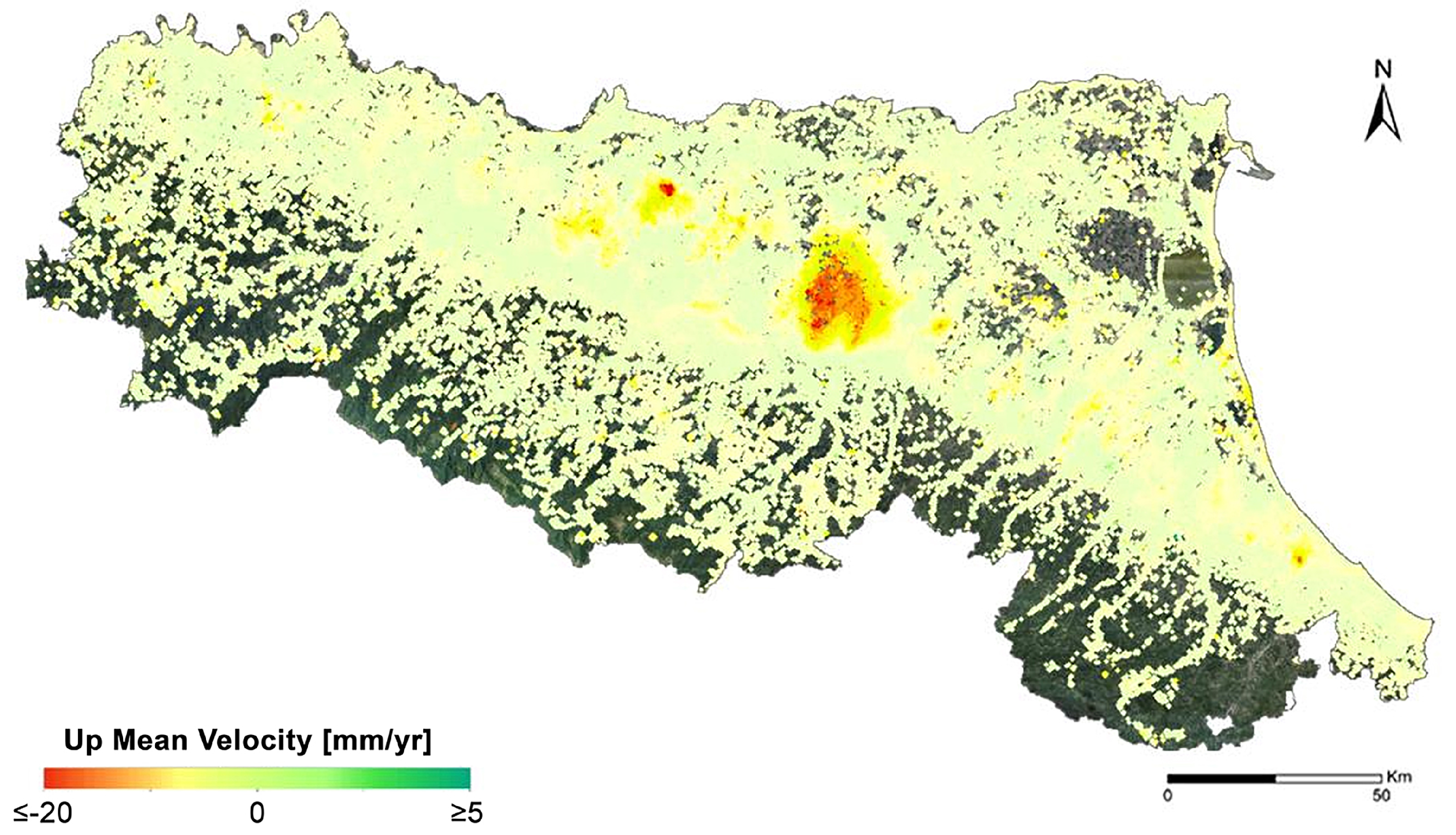
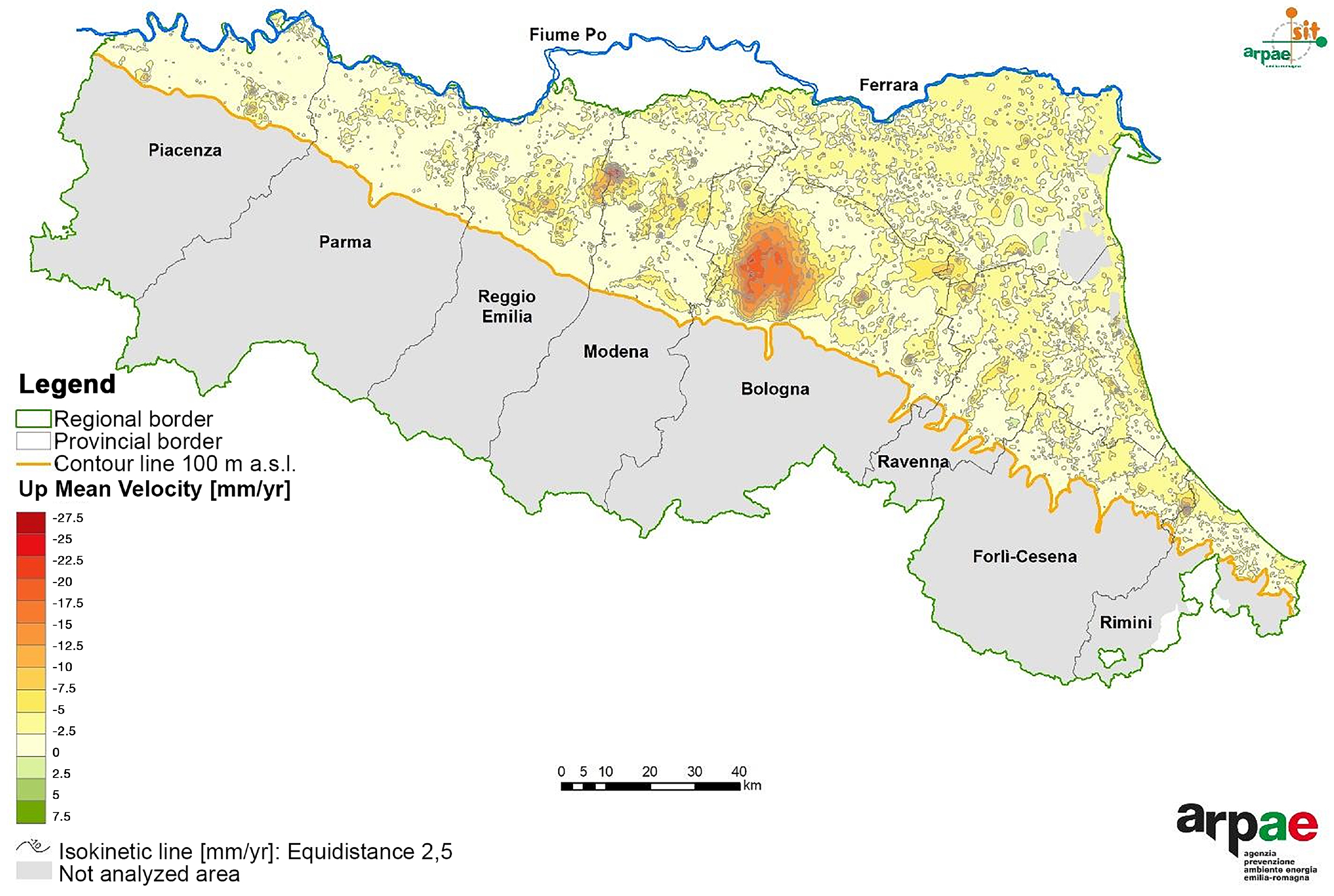
3.6. The 2016–2021 Emilia-Romagna Subsidence Map
- The final dataset of the calibrated interferometric analysis 2016–2021 was used, cropped according to the regional boundary and the 100 m elevation line, with a buffer of 1 km to remove edge effects and outliers, for a total of 552,581 pseudo-MP.
- The spatialization of the data was carried out using the Kriging technique, generating a grid with a mesh size of 100 m × 100 m, co-registered with the grids calculated in the previous monitoring periods, in order to facilitate the comparison of the results in the GIS environment.
- The areas occupied by transitional surface waters, such as the Comacchio Valleys, were excluded from the calculated grid and thus from the final cartography.
- The final cartography was provided via the contour process in a GIS environment, giving isokinetic curves with a step of 2.5 mm/year.
4. Discussion
5. Conclusions
Author Contributions
Funding
Data Availability Statement
Acknowledgments
Conflicts of Interest
Appendix A
| Marker | Longitude | Latitude |
|---|---|---|
| Calibration | ||
| BGDR | 43.8891 | 11.8950 |
| BLGN | 44.5110 | 11.3506 |
| BOBB | 44.7706 | 9.3834 |
| BRAS | 44.1222 | 11.1131 |
| BRIS | 44.2248 | 11.7660 |
| CAST | 44.4316 | 10.4053 |
| CODI | 44.8367 | 12.1120 |
| FERR | 44.8279 | 11.6013 |
| GARI | 44.6769 | 12.2494 |
| GUAS | 44.9178 | 10.6623 |
| ITIM | 44.3475 | 11.7179 |
| MODE | 44.6289 | 10.9487 |
| MSEL | 44.5200 | 11.6465 |
| MTRZ | 44.3128 | 11.4250 |
| PARM | 44.7646 | 10.3122 |
| PIAC | 45.0431 | 9.6897 |
| RAVE | 44.4053 | 12.1919 |
| REGG | 44.7064 | 10.6368 |
| SGIP | 44.6355 | 11.1827 |
| TARO | 44.4879 | 9.7657 |
| VERG | 44.2874 | 11.1105 |
| Validation | ||
| BOL1 | 44.4876 | 11.3288 |
| BOLG | 44.5002 | 11.3568 |
| COLL | 44.7528 | 10.2160 |
| XXX1 | 44.4000 | 12.3000 |
| ITRN | 44.0483 | 12.5821 |
| MOPS | 44.6294 | 10.9492 |
| XXX2 | 44.6000 | 12.3000 |
Appendix B
- the mean velocity of the filtered GNSS data;
- the mean velocity of the selected radar targets around the GNSS station;
- the number of radar targets selected for the calculation of the average speed;
- the relative standard deviation of the average speeds of the selected radar targets;
- the differences used for plan estimation and removal.
| Marker | GNSS [mm/yr] | SqueeSAR® [mm/yr] | SqueeSAR® [mm/yr] | SqueeSAR® MP | [mm/yr] |
|---|---|---|---|---|---|
| BGDR | 0.9 | - | - | 0 | - |
| BLGN | −8.3 | −5.5 | 0.3 | 5 | 2.8 |
| BOBB | −0.6 | 1.1 | 0.5 | 5 | 1.7 |
| BRAS | 0.5 | 0.4 | 0 | 1 | −0.1 |
| BRIS | 0.6 | - | - | 0 | - |
| CAST | 0.8 | 0.7 | 0.2 | 5 | −0.1 |
| CODI | −2.8 | −0.1 | 0.4 | 5 | 2.7 |
| FERR | −1 | 0.2 | 0.3 | 5 | 1.3 |
| GARI | −2.8 | 0 | 0.4 | 5 | 2.8 |
| GUAS | −1.6 | 0.3 | 0.3 | 5 | 2 |
| ITIM | −0.4 | 0.7 | 0.2 | 5 | 1.1 |
| MODE | −4.4 | −0.7 | 0.2 | 5 | 3.8 |
| MSEL | −1.9 | 1.9 | 0.5 | 2 | 3.8 |
| MTRZ | 0 | - | - | 0 | - |
| PARM | −0.1 | 0.9 | 0.8 | 5 | 1 |
| PIAC | −0.7 | 0.2 | 0.2 | 5 | 0.9 |
| RAVE | −3.8 | −0.6 | 0.4 | 5 | 3.2 |
| REGG | −3.2 | −0.1 | 0.2 | 5 | 3.1 |
| SGIP | −7 | −3.5 | 0.9 | 5 | 3.5 |
| TARO | −0.6 | 0.2 | 0.1 | 5 | 0.8 |
| VERG | 0.7 | 1 | 0.1 | 5 | 0.2 |
| Marker | GNSS [mm/yr] | SqueeSAR® [mm/yr] | SqueeSAR® [mm/yr] | SqueeSAR® MP | [mm/yr] |
|---|---|---|---|---|---|
| BGDR | 0.2 | - | - | 0 | - |
| BLGN | −0.9 | −1.8 | 0.3 | 5 | −0.9 |
| BOBB | 0.3 | 0.2 | 0.2 | 5 | −0.2 |
| BRAS | 0 | −0.1 | 0 | 1 | −0.2 |
| BRIS | 1.1 | - | - | 0 | - |
| CAST | 0 | −0.5 | 0.6 | 5 | −0.5 |
| CODI | 0 | −0.3 | 0.6 | 5 | −0.3 |
| FERR | 0.4 | 0 | 0.2 | 5 | −0.3 |
| GARI | −0.3 | −0.3 | 0.3 | 5 | 0 |
| GUAS | 0.1 | −0.1 | 0.1 | 5 | −0.3 |
| ITIM | 0.8 | −0.2 | 0.2 | 5 | −1 |
| MODE | 0.8 | −0.1 | 0.1 | 5 | −0.9 |
| MSEL | 0.9 | 0.6 | 0 | 2 | −0.3 |
| MTRZ | 1.5 | - | - | 0 | - |
| PARM | 0.8 | 0.2 | 0.4 | 5 | −0.6 |
| PIAC | 0.1 | −0.1 | 0.1 | 5 | −0.3 |
| RAVE | 0.3 | 0 | 0.6 | 5 | −0.3 |
| REGG | −0.2 | 0.3 | 0.2 | 5 | 0.5 |
| SGIP | 1.5 | 1.4 | 1.1 | 5 | −0.1 |
| TARO | 0.2 | 0.1 | 0.2 | 5 | −0.1 |
| VERG | 1.8 | 0.5 | 0.2 | 5 | −1.3 |
References
- Loupasakis, C.; Rozos, D. Finite-Element Simulation of Land Subsidence Induced by Water Pumping in Kalochori Village, Greece. Q. J. Eng. Geol. Hydrogeol. 2009, 42, 369–382. [Google Scholar] [CrossRef]
- Galloway, D.L.; Burbey, T.J. Review: Regional Land Subsidence Accompanying Groundwater Extraction. Hydrogeol. J. 2011, 19, 1459–1486. [Google Scholar] [CrossRef]
- Herrera-García, G.; Ezquerro, P.; Tomás, R.; Béjar-Pizarro, M.; López-Vinielles, J.; Rossi, M.; Mateos, R.M.; Carreón-Freyre, D.; Lambert, J.; Teatini, P.; et al. Mapping the Global Threat of Land Subsidence. Science 2021, 371, 34–36. [Google Scholar] [CrossRef] [PubMed]
- Candela, T.; Koster, K. The Many Faces of Anthropogenic Subsidence. Science 2022, 376, 1381–1382. [Google Scholar] [CrossRef] [PubMed]
- Tzampoglou, P.; Ilia, I.; Karalis, K.; Tsangaratos, P.; Zhao, X.; Chen, W. Selected Worldwide Cases of Land Subsidence Due to Groundwater Withdrawal. Water 2023, 15, 1094. [Google Scholar] [CrossRef]
- Bagheri-Gavkosh, M.; Hosseini, S.M.; Ataie-Ashtiani, B.; Sohani, Y.; Ebrahimian, H.; Morovat, F.; Ashrafi, S. Land Subsidence: A Global Challenge. Sci. Total Environ. 2021, 778, 146193. [Google Scholar] [CrossRef]
- Ohenhen, L.O.; Shirzaei, M.; Barnard, P.L. Slowly but Surely: Exposure of Communities and Infrastructure to Subsidence on the US East Coast. PNAS Nexus 2023, 3, pgad426. [Google Scholar] [CrossRef]
- Huning, L.S.; Love, C.A.; Anjileli, H.; Vahedifard, F.; Zhao, Y.; Chaffe, P.L.B.; Cooper, K.; Alborzi, A.; Pleitez, E.; Martinez, A.; et al. Global Land Subsidence: Impact of Climate Extremes and Human Activities. Rev. Geophys. 2024, 62, e2023RG000817. [Google Scholar] [CrossRef]
- Xu, Y.; Wu, Z.; Zhang, H.; Liu, J.; Jing, Z. Land Subsidence Monitoring and Building Risk Assessment Using InSAR and Machine Learning in a Loess Plateau City—A Case Study of Lanzhou, China. Remote Sens. 2023, 15, 2851. [Google Scholar] [CrossRef]
- Jin, B.; Zeng, T.; Wang, T.; Zhang, Z.; Gui, L.; Yin, K.; Zhao, B. Advanced Risk Assessment Framework for Land Subsidence Impacts on Transmission Towers in Salt Lake Region. Environ. Model. Softw. 2024, 177, 106058. [Google Scholar] [CrossRef]
- He, Y.; Li, X.; Yang, J.; Liu, Y.; Yang, G.; Hu, M.; Chen, S.; Yao, H.; Wang, L.; Xiong, X. Urban Land Subsidence Monitoring and Risk Assessment Using the Point Target Based SBAS-InSAR Method: A Case Study of Changsha City. Remote Sens. Lett. 2024, 15, 689–699. [Google Scholar] [CrossRef]
- Brandt, J.T.; Sneed, M.; Danskin, W.R. Detection and Measurement of Land Subsidence and Uplift Using Interferometric Synthetic Aperture Radar, San Diego, California, USA, 2016–2018. Proc. Int. Assoc. Hydrol. Sci. 2020, 382, 45–49. [Google Scholar] [CrossRef]
- Zhu, Z.; Qiu, S.; Ye, S. Remote Rensing of Land Change: A MUltifaceted Perspective. Remote Sens. Environ. 2022, 282, 113266. [Google Scholar] [CrossRef]
- Ghorbani, Z.; Khosravi, A.; Maghsoudi, Y.; Mojtahedi, F.F.; Javadnia, E.; Nazari, A. Use of InSAR Data for Measuring Land Subsidence Induced by Groundwater Withdrawal and Climate Change in Ardabil Plain, Iran. Sci. Rep. 2022, 12, 13998. [Google Scholar] [CrossRef]
- Dacome, M.C.; Miandro, R.; Vettorel, M.; Roncari, G. Subsidence Monitoring Network: An Italian Example Aimed at a Sustainable Hydrocarbon E&P Activity. Proc. Int. Assoc. Hydrol. Sci. 2015, 372, 379–384. [Google Scholar] [CrossRef]
- Teatini, P.; Ferronato, M.; Gambolati, G.; Bertoni, W.; Gonella, M. A Century of Land Subsidence in Ravenna, Italy. Environ. Geol. 2005, 47, 831–846. [Google Scholar] [CrossRef]
- Demoulin, A.; Collignon, A. Nature of the Recent Vertical Ground Movements Inferred from High-Precision Leveling Data in an Intraplate Setting: NE Ardenne, Belgium. J. Geophys. Res. Solid Earth 2000, 105, 693–705. [Google Scholar] [CrossRef]
- Gleason, S. GNSS Applications and Methods, 1st ed.; Artech House: Norwood, MA, USA, 2009. [Google Scholar]
- Petropoulos, G.P.; Srivastava, P.K. (Eds.) GPS and GNSS Technology in Geosciences; Elsevier: Amsterdam, The Netherlands; Oxford, UK; Cambridge, MA, USA, 2021. [Google Scholar]
- Tao, Q.; Li, X.; Gao, T.; Chen, Y.; Liu, R.; Xiao, Y. Land Subsidence Monitoring and Analysis in Qingdao, China Using Time Series InSAR Combining PS and DS. Geomat. Nat. Hazards Risk 2025, 16, 2447543. [Google Scholar] [CrossRef]
- Navarro-Hernández, M.I.; Tomás, R.; Valdes-Abellan, J.; Bru, G.; Ezquerro, P.; Guardiola-Albert, C.; Elçi, A.; Batkan, E.A.; Caylak, B.; Ören, A.H.; et al. Monitoring land subsidence Induced by Tectonic Activity and Groundwater Extraction in the Eastern Gediz River Basin (Türkiye) Using Sentinel-1 Observations. Eng. Geol. 2023, 327, 107343. [Google Scholar] [CrossRef]
- Giorgini, E.; Vecchi, E.; Poluzzi, L.; Tavasci, L.; Barbarella, M.; Gandolfi, S. 15 years of the Italian GNSS Geodetic Reference Frame (RDN): Preliminary analysis and considerations. In Geomatics for Green and Digital Transition; Borgogno-Mondino, E., Zamperlin, P., Eds.; Springer International Publishing: Cham, Switzerland, 2022; Volume 1651, pp. 3–14. [Google Scholar] [CrossRef]
- Parizzi, A.; Rodriguez Gonzalez, F.; Brcic, R. A Covariance-Based Approach to Merging InSAR and GNSS Displacement Rate Measurements. Remote Sens. 2020, 12, 300. [Google Scholar] [CrossRef]
- Ferretti, A.; Fumagalli, A.; Passera, E.; Rucci, A. Insar Data Calibration in Wide Area Processing. In Proceedings of the IGARSS 2022—2022 IEEE International Geoscience and Remote Sensing Symposium, Kuala Lumpur, Malaysia, 17–22 July 2022; pp. 5101–5104. [Google Scholar] [CrossRef]
- Hanssen, R.F. Radar Interferometry Data Interpretation and Error Analysis; Remote Sensing and Digital Image Processing; Springer: Dordrecht, The Netherlands, 2001; Volume 2. [Google Scholar] [CrossRef]
- Watson, A.R.; Elliott, J.R.; Lazecký, M.; Maghsoudi, Y.; McGrath, J.D.; Walters, R.J. An InSAR-GNSS Velocity Field for Iran. Geophys. Res. Lett. 2024, 51, e2024GL108440. [Google Scholar] [CrossRef]
- Hussain, E.; Wright, T.J.; Walters, R.J.; Bekaert, D.; Hooper, A.; Houseman, G.A. Geodetic Observations of Postseismic Creep in the Decade After the 1999 Izmit Earthquake, Turkey: Implications for a Shallow Slip Deficit. J. Geophys. Res. Solid Earth 2016, 121, 2980–3001. [Google Scholar] [CrossRef]
- Weiss, J.R.; Walters, R.J.; Morishita, Y.; Wright, T.J.; Lazecky, M.; Wang, H.; Hussain, E.; Hooper, A.J.; Elliott, J.R.; Rollins, C.; et al. High-Resolution Surface Velocities and Strain for Anatolia From Sentinel-1 InSAR and GNSS Data. Geophys. Res. Lett. 2020, 47, e2020GL087376. [Google Scholar] [CrossRef]
- Raspini, F.; Caleca, F.; Del Soldato, M.; Festa, D.; Confuorto, P.; Bianchini, S. Review of Satellite Radar Interferometry for Subsidence Analysis. Earth-Sci. Rev. 2022, 235, 104239. [Google Scholar] [CrossRef]
- Fabris, M.; Battaglia, M.; Chen, X.; Menin, A.; Monego, M.; Floris, M. An Integrated InSAR and GNSS Approach to Monitor Land Subsidence in the Po River Delta (Italy). Remote Sens. 2022, 14, 5578. [Google Scholar] [CrossRef]
- Costantini, M.; Ferretti, A.; Minati, F.; Falco, S.; Trillo, F.; Colombo, D.; Novali, F.; Malvarosa, F.; Mammone, C.; Vecchioli, F.; et al. Analysis of Surface Deformations Over the Whole Italian Territory by Interferometric Processing of ERS, Envisat and COSMO-SkyMed radar data. Remote Sens. Environ. 2017, 202, 250–275. [Google Scholar] [CrossRef]
- Giorgini, E.; Orellana, F.; Arratia, C.; Tavasci, L.; Montalva, G.; Moreno, M.; Gandolfi, S. InSAR Monitoring Using Persistent Scatterer Interferometry (PSI) and Small Baseline Subset (SBAS) Techniques for Ground Deformation Measurement in Metropolitan Area of Concepción, Chile. Remote Sens. 2023, 15, 5700. [Google Scholar] [CrossRef]
- Chen, D.; Wu, Q.; Sun, Z.; Shi, X.; Zhang, S.; Zhang, Y.; Wu, Y. Semi-Automatic Detection of Ground Displacement from Multi-Temporal Sentinel-1 Synthetic Aperture Radar Interferometry Analysis and Density-Based Spatial Clustering of Applications with Noise in Xining City, China. Remote Sens. 2024, 16, 3066. [Google Scholar] [CrossRef]
- Livani, M.; Petracchini, L.; Benetatos, C.; Marzano, F.; Billi, A.; Carminati, E.; Doglioni, C.; Petricca, P.; Maffucci, R.; Codegone, G.; et al. Subsurface Geological and Geophysical Data from the Po Plain and the Northern Adriatic Sea (north Italy). Earth Syst. Sci. Data 2023, 15, 4261–4293. [Google Scholar] [CrossRef]
- Severi, P. Soil Uplift in the Emilia-Romagna Plain (Italy) by Satellite Radar Interferometry. Bull. Geophys. Oceanogr. 2021, 62, 527–542. [Google Scholar] [CrossRef]
- Margheriti, L.; Pondrelli, S.; Piccinini, D.; Agostinetti, N.P.; Giovani, L.; Salimbeni, S.; Lucente, F.P.; Amato, A.; Baccheschi, P.; Park, J. The Subduction Structure of the Northern Apennines: Results from the RETREAT Seismic Deployment. Ann. Geophys. 2009, 49, 1119–1131. [Google Scholar] [CrossRef]
- Colantoni, P.; Gallignani, P.; Lenaz, R. Late Pleistocene and Holocene Evolution of the North Adriatic Continental Shelf (Italy). Mar. Geol. 1979, 33, M41–M50. [Google Scholar] [CrossRef]
- Lucente, F.P.; Speranza, F. Belt Bending Driven by Lateral Bending of Subducting Lithospheric Slab: Geophysical Evidences from the Northern Apennines (Italy). Tectonophysics 2001, 337, 53–64. [Google Scholar] [CrossRef]
- Speranza, F.; Sagnotti, L.; Mattei, M. Tectonics of the Umbria-Marche-Romagna Arc (central northern Apennines, Italy): New paleomagnetic constraints. J. Geophys. Res. Solid Earth 1997, 102, 3153–3166. [Google Scholar] [CrossRef]
- Lucente, F.P.; Chiarabba, C.; Cimini, G.B.; Giardini, D. Tomographic Constraints on the Geodynamic Evolution of the Italian Region. J. Geophys. Res. Solid Earth 1999, 104, 20307–20327. [Google Scholar] [CrossRef]
- Zuccarini, A.; Giacomelli, S.; Severi, P.; Berti, M. Long-Term Spatiotemporal Evolution of Land SUubsidence in the Urban Area of Bologna, Italy. Bull. Eng. Geol. Environ. 2024, 83, 35. [Google Scholar] [CrossRef]
- Caputo, M.; Pieri, L.; Unguendoli, M. Geometric Investigation of the Subsidence in the Po Delta. In Bollettino di Geofisica Teorica e Applicata; IGM: Florence, Italy, 1970; Volume 13, pp. 187–207. [Google Scholar]
- Donaldson, E.C.; Chilingarian, G.V.; Fu Yen, T. Chapter 1 Introduction to compaction/subsidence—Introduction to tectonics and sedimentation. In Developments in Petroleum Science; Elsevier: Amsterdam, The Netherlands, 1995; Volume 41, pp. 1–45. [Google Scholar] [CrossRef]
- Eid, C.; Benetatos, C.; Rocca, V. Fluid Production Dataset for the Assessment of the Anthropogenic Subsidence in the Po Plain Area (Northern Italy). Resources 2022, 11, 53. [Google Scholar] [CrossRef]
- Carbognin, L.; Tosi, L. Interaction between Climate Changes, Eustacy and Land Subsidence in the North Adriatic Region, Italy. Mar. Ecol. 2002, 23, 38–50. [Google Scholar] [CrossRef]
- Gambolati, G. Cenas Coastline Evolution of the Upper Adriatic Sea Due to Sea Level Rise and Natural and Anthropogenic Land Subsidence; Number v.28 in Water Science and Technology Library; Springer: Dordrecht, The Netherlands, 1998. [Google Scholar]
- Bitelli, G.; Bonsignore, F.; Pellegrino, I.; Vittuari, L. Evolution of the Techniques for Subsidence Monitoring at Regional Scale: The Case of Emilia-Romagna Region (Italy). Proc. Int. Assoc. Hydrol. Sci. 2015, 372, 315–321. [Google Scholar] [CrossRef]
- Bitelli, G.; Bonsignore, F.; Unguendoli, M. Levelling and GPS Networks to Monitor Ground Subsidence in the Southern Po Valley. J. Geodyn. 2000, 30, 355–369. [Google Scholar] [CrossRef]
- Bitelli, G.; Bonsignore, F.; Del Conte, S.; Franci, F.; Lambertini, A.; Novali, F.; Severi, P.; Vittuari, L. Updating the Subsidence Map of Emilia-Romagna Region (Italy) by Integration of SAR Interferometry and GNSS Time Series: The 2011–2016 Period. Proc. Int. Assoc. Hydrol. Sci. 2020, 382, 39–44. [Google Scholar] [CrossRef]
- Panetti, A.; Rostan, F.; L’Abbate, M.; Bruno, C.; Bauleo, A.; Catalano, T.; Cotogni, M.; Galvagni, L.; Pietropaolo, A.; Taini, G.; et al. Copernicus Sentinel-1 Satellite and C-SAR instrument. In Proceedings of the 2014 IEEE Geoscience and Remote Sensing Symposium, Quebec City, QC, Canada, 13–18 July 2014; pp. 1461–1464. [Google Scholar] [CrossRef]
- De Zan, F.; Monti Guarnieri, A. TOPSAR: Terrain Observation by Progressive Scans. IEEE Trans. Geosci. Remote Sens. 2006, 44, 2352–2360. [Google Scholar] [CrossRef]
- Potin, P.; Rosich, B.; Miranda, N.; Grimont, P.; Shurmer, I.; O’Connell, A.; Krassenburg, M.; Gratadour, J.B. Copernicus Sentinel-1 Constellation Mission Operations Status. In Proceedings of the IGARSS 2019—2019 IEEE International Geoscience and Remote Sensing Symposium, Yokohama, Japan, 28 July–2 August 2019; pp. 5385–5388. [Google Scholar] [CrossRef]
- Fuhrmann, T.; Garthwaite, M.C. Resolving Three-Dimensional Surface Motion with InSAR: Constraints from Multi-Geometry Data Fusion. Remote Sens. 2019, 11, 241. [Google Scholar] [CrossRef]
- Grandin, R. Interferometric Processing of SLC Sentinel-1 TOPS Data. In Proceedings of the Fringe 2015: Advances in the Science and Applications of SAR Interferometry and Sentinel-1 InSAR Workshop, Frascati, Italy, 23–27 March 2015; European Space Agency: Frascati, Italy, 2015. [Google Scholar] [CrossRef]
- Ferretti, A.; Fumagalli, A.; Novali, F.; Prati, C.; Rocca, F.; Rucci, A. A New Algorithm for Processing Interferometric Data-Stacks: SqueeSAR. IEEE Trans. Geosci. Remote Sens. 2011, 49, 3460–3470. [Google Scholar] [CrossRef]
- Ferretti, A.; Prati, C.; Rocca, F. Permanent scatterers in SAR interferometry. IEEE Trans. Geosci. Remote Sens. 2001, 39, 8–20. [Google Scholar] [CrossRef]
- Stoica, P.; Selen, Y. Model-order selection. IEEE Signal Process. Mag. 2004, 21, 36–47. [Google Scholar] [CrossRef]
- Zumberge, J.F.; Heflin, M.B.; Jefferson, D.C.; Watkins, M.M.; Webb, F.H. Precise Point Positioning for the Efficient and Robust Analysis of GPS Data from Large N etworks. J. Geophys. Res. Solid Earth 1997, 102, 5005–5017. [Google Scholar] [CrossRef]
- Gandolfi, S.; Tavasci, L.; Poluzzi, L. Improved PPP Performance in Regional Networks. GPS Solut. 2016, 20, 485–497. [Google Scholar] [CrossRef]
- Blewitt, G.; Lavallée, D. Effect of Annual Signals on Geodetic Velocity. J. Geophys. Res. Solid Earth 2002, 107, ETG 9-1–ETG 9-11. [Google Scholar] [CrossRef]
- Barbarella, M.; Gandolfi, S.; Poluzzi, L.; Tavasci, L. Precision of PPP as a Function of the Observing-Session Duration. IEEE Trans. Aerosp. Electron. Syst. 2018, 54, 2827–2836. [Google Scholar] [CrossRef]
- Boehm, J.; Werl, B.; Schuh, H. Troposphere Mapping Functions for GPS and Very Long Baseline Interferometry from European Centre for Medium-Range Weather Forecasts Operational Analysis Data. J. Geophys. Res. Solid Earth 2006, 111, 2005JB003629. [Google Scholar] [CrossRef]
- Altamimi, Z. EUREF Technical Note 1: Relationship and Transformation Between the International and the European Terrestrial Reference Systems; Technical Report; Institut National de l’Information Géographique et Forestière (IGN): Forestière, France, 2024. [Google Scholar]
- Bischoff, C.A.; Ferretti, A.; Novali, F.; Uttini, A.; Giannico, C.; Meloni, F. Nationwide Deformation Monitoring with SqueeSAR® using Sentinel-1 Data. Proc. Int. Assoc. Hydrol. Sci. 2020, 382, 31–37. [Google Scholar] [CrossRef]
- Herring, T. MATLAB Tools for viewing GPS velocities and time series. GPS Solut. 2003, 7, 194–199. [Google Scholar] [CrossRef]
- Ferretti, A.; Savio, G.; Barzaghi, R.; Borghi, A.; Musazzi, S.; Novali, F.; Prati, C.; Rocca, F. Submillimeter Accuracy of InSAR Time Series: Experimental Validation. IEEE Trans. Geosci. Remote Sens. 2007, 45, 1142–1153. [Google Scholar] [CrossRef]
- Stramondo, S.; Saroli, M.; Tolomei, C.; Moro, M.; Doumaz, F.; Pesci, A.; Loddo, F.; Baldi, P.; Boschi, E. Surface movements in Bologna (Po Plain—Italy) detected by multitemporal DInSAR. Remote Sens. Environ. 2007, 110, 304–316. [Google Scholar] [CrossRef]
- Marcaccio, M.M.M. Monitoraggio dei Movimenti Verticali del Suolo e Aggiornamento Della Cartografia di Subsidenza Nella Pianura dell’Emilia-Romagna. Periodo 2016–2021; Technical Report; Regione Emilia–Romagna, Arpae Emilia-Romagna: Bologna, Italy, 2023. [Google Scholar]
- Bissoli, R.P.I. Rilievo Della Subsidenza Nella Pianura Emiliano–Romagnola. Relazione Finale, Seconda Fase; Technical Report; Regione Emilia–Romagna, Arpa Emilia-Romagna: Bologna, Italy, 2018. [Google Scholar]


| Track | Orbit | Incidence Angle | Acquisitions | Period |
|---|---|---|---|---|
| T117 | Ascending | 307 | 12 January 2016–26 June 2021 | |
| T95 | Descending | 297–301 | 11 January 2016–25 June 2021 | |
| T15 | Ascending | 288–293 | 17 January 2016–25 June 2021 | |
| T168 | Descending | 306–307 | 16 January 2016–30 June 2021 |
| Marker | [mm/yr] | [mm/yr] | [mm/yr] | [mm/yr] | [mm/yr] | [mm/yr] |
|---|---|---|---|---|---|---|
| Calibration | ||||||
| BGDR | 2.1 | 0.04 | 0.24 | 0.03 | 0.98 | 0.05 |
| BLGN | 5.68 | 0.02 | −0.81 | 0.02 | −8.25 | 0.05 |
| BOBB | 1.09 | 0.01 | 0.31 | 0.01 | −0.54 | 0.04 |
| BRAS | 1.65 | 0.02 | 0.09 | 0.01 | 0.48 | 0.04 |
| BRIS | 3.41 | 0.02 | 1.09 | 0.01 | 0.63 | 0.05 |
| CAST | 1.76 | 0.02 | 0.09 | 0.01 | 0.83 | 0.05 |
| CODI | 2.19 | 0.01 | 0.01 | 0.01 | −2.81 | 0.03 |
| FERR | 2.56 | 0.01 | 0.39 | 0.01 | −1.12 | 0.03 |
| GARI | 1.29 | 0.01 | −0.28 | 0.01 | −2.75 | 0.04 |
| GUAS | 1.81 | 0.01 | 0.1 | 0.01 | −1.65 | 0.05 |
| ITIM | 3.46 | 0.01 | 0.82 | 0.01 | −0.37 | 0.03 |
| MODE | 2.83 | 0.01 | 0.82 | 0.01 | −4.1 | 0.04 |
| MSEL | 2.81 | 0.01 | 0.92 | 0.01 | −1.83 | 0.03 |
| MTRZ | 3.83 | 0.02 | 1.57 | 0.02 | −0.85 | 0.08 |
| PARM | 1.86 | 0.01 | 0.75 | 0.01 | −0.3 | 0.05 |
| PIAC | 1.41 | 0.01 | 0.16 | 0.01 | −0.71 | 0.03 |
| RAVE | 2.94 | 0.01 | 0.31 | 0.01 | −3.75 | 0.04 |
| REGG | 2.35 | 0.01 | −0.23 | 0.01 | −3.12 | 0.04 |
| SGIP | 3.11 | 0.01 | 1.49 | 0.02 | −6.97 | 0.04 |
| TARO | 1.12 | 0.01 | 0.29 | 0.01 | −0.58 | 0.05 |
| VERG | 2.53 | 0.01 | 1.86 | 0.01 | 1 | 0.05 |
| Validation | ||||||
| BOL1 | 4.17 | 0.02 | 0.37 | 0.01 | −0.32 | 0.04 |
| BOLG | 4.14 | 0.02 | 0.32 | 0.02 | −2.04 | 0.06 |
| COLL | 1.59 | 0.02 | 1.25 | 0.02 | −2.33 | 0.05 |
| XXX1 | 2.39 | 0.01 | 3.27 | 0.02 | −8.71 | 0.04 |
| ITRN | 3.94 | 0.01 | 0.95 | 0.03 | −1.23 | 0.04 |
| MOPS | 3.17 | 0.01 | 0.73 | 0.02 | −3.92 | 0.04 |
| XXX2 | 2.7 | 0.02 | −0.6 | 0.02 | −3.72 | 0.06 |
| Marker | GNSS [mm/yr] | SqueeSAR® [mm/yr] | [mm/yr] |
|---|---|---|---|
| BOL1 | −0.3 | −1.8 | 1.5 |
| BOLG | −2 | −2.8 | 0.8 |
| COLL | −2.3 | −1.1 | −1.2 |
| XXX1 | −8.7 | −6.7 | −2 |
| ITRN | −1.2 | −2.2 | 1 |
| MOPS | −3.9 | −2.7 | −1.2 |
| XXX2 | −3.7 | −3.7 | 0 |
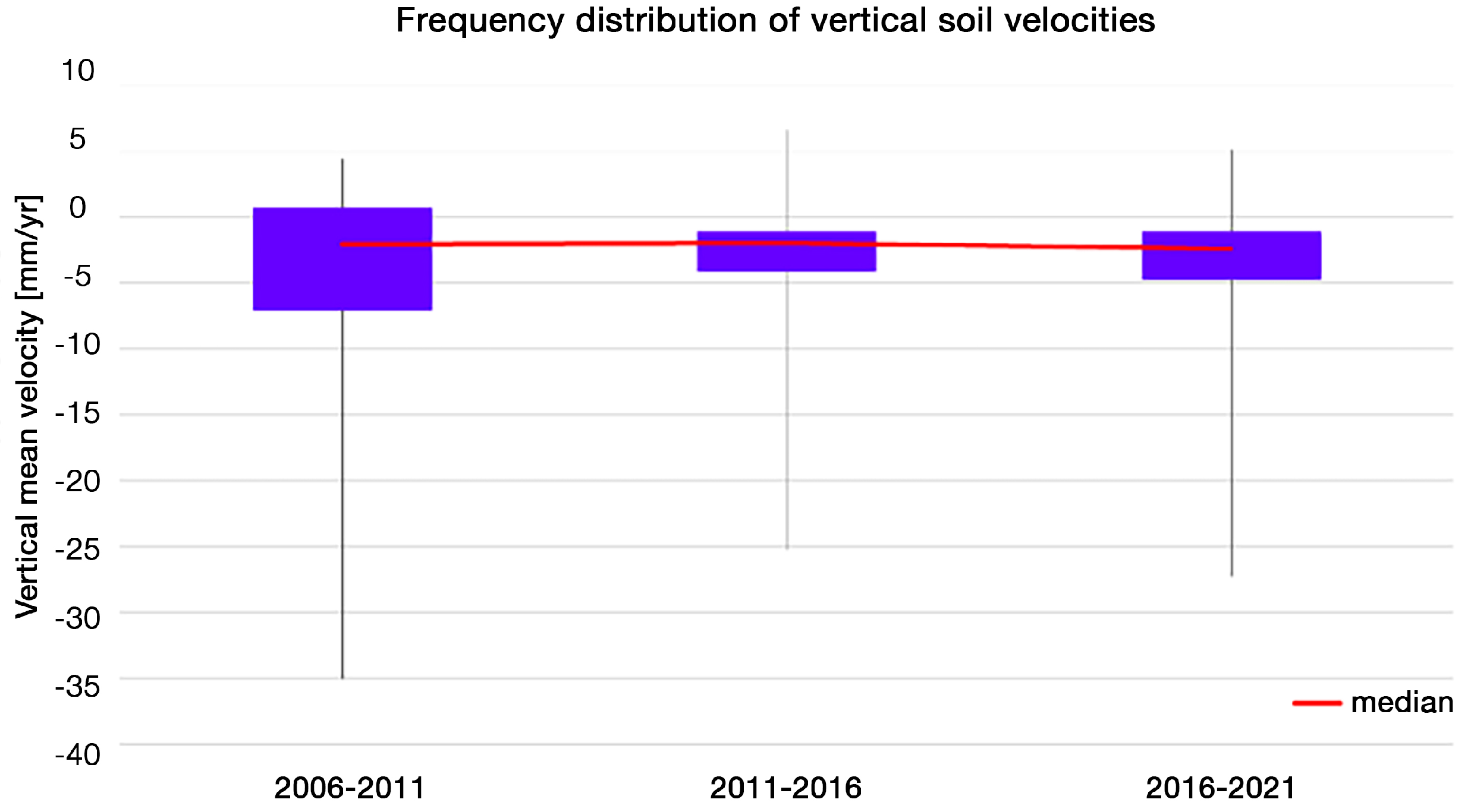
| Maximum | Percentile | Median | Percentile | Minimum | |
|---|---|---|---|---|---|
| 2006–2011 | 4.42 | 0.70 | −2.00 | −7.08 | −35.05 |
| 2011–2016 | 6.63 | −1.13 | −1.93 | −4.05 | −25.24 |
| 2016–2021 | 5.15 | −1.13 | −2.37 | −4.75 | −27.29 |
Disclaimer/Publisher’s Note: The statements, opinions and data contained in all publications are solely those of the individual author(s) and contributor(s) and not of MDPI and/or the editor(s). MDPI and/or the editor(s) disclaim responsibility for any injury to people or property resulting from any ideas, methods, instructions or products referred to in the content. |
© 2025 by the authors. Licensee MDPI, Basel, Switzerland. This article is an open access article distributed under the terms and conditions of the Creative Commons Attribution (CC BY) license (https://creativecommons.org/licenses/by/4.0/).
Share and Cite
Bitelli, G.; Ferretti, A.; Giannico, C.; Giorgini, E.; Lambertini, A.; Marcaccio, M.; Mazzei, M.; Vittuari, L. Subsidence Monitoring in Emilia-Romagna Region (Italy) from 2016 to 2021: From InSAR and GNSS Integration to Data Analysis. Remote Sens. 2025, 17, 947. https://doi.org/10.3390/rs17060947
Bitelli G, Ferretti A, Giannico C, Giorgini E, Lambertini A, Marcaccio M, Mazzei M, Vittuari L. Subsidence Monitoring in Emilia-Romagna Region (Italy) from 2016 to 2021: From InSAR and GNSS Integration to Data Analysis. Remote Sensing. 2025; 17(6):947. https://doi.org/10.3390/rs17060947
Chicago/Turabian StyleBitelli, Gabriele, Alessandro Ferretti, Chiara Giannico, Eugenia Giorgini, Alessandro Lambertini, Marco Marcaccio, Marianna Mazzei, and Luca Vittuari. 2025. "Subsidence Monitoring in Emilia-Romagna Region (Italy) from 2016 to 2021: From InSAR and GNSS Integration to Data Analysis" Remote Sensing 17, no. 6: 947. https://doi.org/10.3390/rs17060947
APA StyleBitelli, G., Ferretti, A., Giannico, C., Giorgini, E., Lambertini, A., Marcaccio, M., Mazzei, M., & Vittuari, L. (2025). Subsidence Monitoring in Emilia-Romagna Region (Italy) from 2016 to 2021: From InSAR and GNSS Integration to Data Analysis. Remote Sensing, 17(6), 947. https://doi.org/10.3390/rs17060947