Evaluation and Optimization Strategies for Forest Landscape Stability in Different Landform Types of the Loess Plateau

Abstract

This study aims to develop a forest landscape stability assessment framework that integrates structure, function, and resilience to assess forest landscape stability under different landform types on the Loess Plateau, and to propose differentiated optimization strategies. Remote sensing images and ground survey data were combined to compare the effectiveness of different machine learning models in aboveground biomass (AGB) inversion. Meanwhile, forest fragmentation and landscape multifunctionality were assessed, and a Landscape Stability Index (LSI) was proposed to quantify regional forest landscape stability. The main findings are as follows: (1) between 2000 and 2022, the degree of forest fragmentation and multifunctionality in the hilly gully region improved significantly, and the Simpson’s Diversity Index (SDI) value showed an increasing trend; the plateau gully region showed a decreasing trend in the SDI value. The degree of forest fragmentation in the hilly gully region was higher and showed significant changes, while the plateau gully region was more stable, with the “Interior” and “Dominant” types dominating. (2) The eXtreme Gradient Boosting model outperformed other models in AGB estimation, with R² = 0.81 and RMSE = 24.67 ton ha⁻¹. (3) The LSI of the hilly gully region generally increased, especially in Yanchang, showing a significant increase in ecological stability; the LSI of the plateau gully region generally decreased, especially in Baishui, showing a trend of weakening stability. Based on the assessment results, optimization strategies for different stabilities were proposed, including the hierarchical management of fragmentation, multi-objective management to improve the SDI, and adaptive management for AGB. The forest landscape stability assessment framework proposed in this study can effectively assess the stability of forest landscapes, reveal the differences in ecological restoration in different regions, and provide new perspectives and strategies for forest landscape management and optimization in the Loess Plateau.

1. Introduction

In landscape ecology, landscape stability refers to the ability of a landscape to maintain its structural, functional, and dynamic balance when facing external disturbances such as natural disasters or human activities [1,2]. Forest landscape stability not only reflects the health and functional integrity of forest ecosystems but also determines their resilience and recovery capacity in the face of external disturbances [3,4]. However, with the increasing impacts of climate change and human activities on forest landscapes, forest landscapes’ stability is facing unprecedented challenges [5,6]. Therefore, assessing and optimizing the stability of forest landscapes has become a key issue in landscape ecology research, especially in the process of ecological restoration and landscape optimization strategies.

The Loess Plateau, an important ecological barrier in China, covers a large area in the central and northern parts of the country. Due to its unique geographical and climatic conditions, this region has long faced a series of serious ecological problems, such as soil erosion, vegetation degradation, and desertification [7,8]. In the early 1990s, the government implemented large-scale ecological restoration projects (such as conversion of farmland to forest and protection natural forests), which effectively increased forest cover [9]. Despite the significant ecological restoration effects achieved, scientific assessments of forest landscape stability in this region, particularly at the landscape level, are still lacking. The region has a complex topography with a network of gullies, mainly consisting of plateau gully and hilly gully landforms. Forest landscapes under different landform types show significant differences in structure, function, and resilience, which poses special challenges for the assessment and optimization of regional ecosystem stability [10,11]. However, systematic research on the effects of different landform types on forest landscape stability is still lacking, and there is an urgent need to establish a comprehensive assessment framework to fill this research gap.

In recent years, significant progress has been made in research methods and strategies for assessing forest landscape stability. Researchers have approached this topic from multiple angles, including remote sensing technology, multi-scale ecological analysis, machine learning modeling, landscape pattern assessment, and natural disaster prediction. By using landscape pattern indicators [12,13], landscape dynamic models [14], disturbance simulations [15], and ecological network analysis [16], these studies have revealed the spatial–temporal characteristics of landscape patterns and structures and quantitatively assessed landscape stability. However, existing studies predominantly focus on the stability assessment of a single dimension, overlooking the comprehensive impact of different landform types on forest landscape stability. Systematic evaluation and targeted optimization strategies are lacking. This limits a comprehensive understanding of regional ecosystem stability and effective management.

Forest fragmentation, as a key factor influencing the stability of landscape structure, directly affects the connectivity of forest ecosystems and the maintenance of biodiversity [17,18]. The degree of fragmentation and its dynamic trends vary considerably among different landform types [19]. Furthermore, the diversity and comprehensiveness of ecosystem services are also important dimensions for assessing forest landscape stability [20]. In addition, biomass, as an important indicator of ecosystem resilience, may intuitively reflect the carbon storage capacity and growth status of the forest, thus indicating its ability to withstand and recover from disturbances [21]. In the context of the Loess Plateau, the lack of a comprehensive assessment framework that simultaneously considers landscape structure, function, and resilience represents a critical research gap that urgently needs to be addressed through systematic integration.

Based on this background, this study aims to develop a framework for forest landscape stability assessment that integrates structure, function, and resilience, while considering the stability and optimization strategies of forest landscapes across different landform types in the Loess Plateau. The research will use remote sensing imagery and field survey data, and apply machine learning models to invert forest AGB. It will combine the degree of forest fragmentation and landscape multifunctionality indices to comprehensively quantify the overall level of stability of regional forest landscapes. By constructing this assessment framework, this study will provide refined, targeted recommendations for subsequent ecological restoration projects and management authorities, thus laying a scientific foundation for ensuring regional ecological security and sustainable development.

2. Materials and Methods

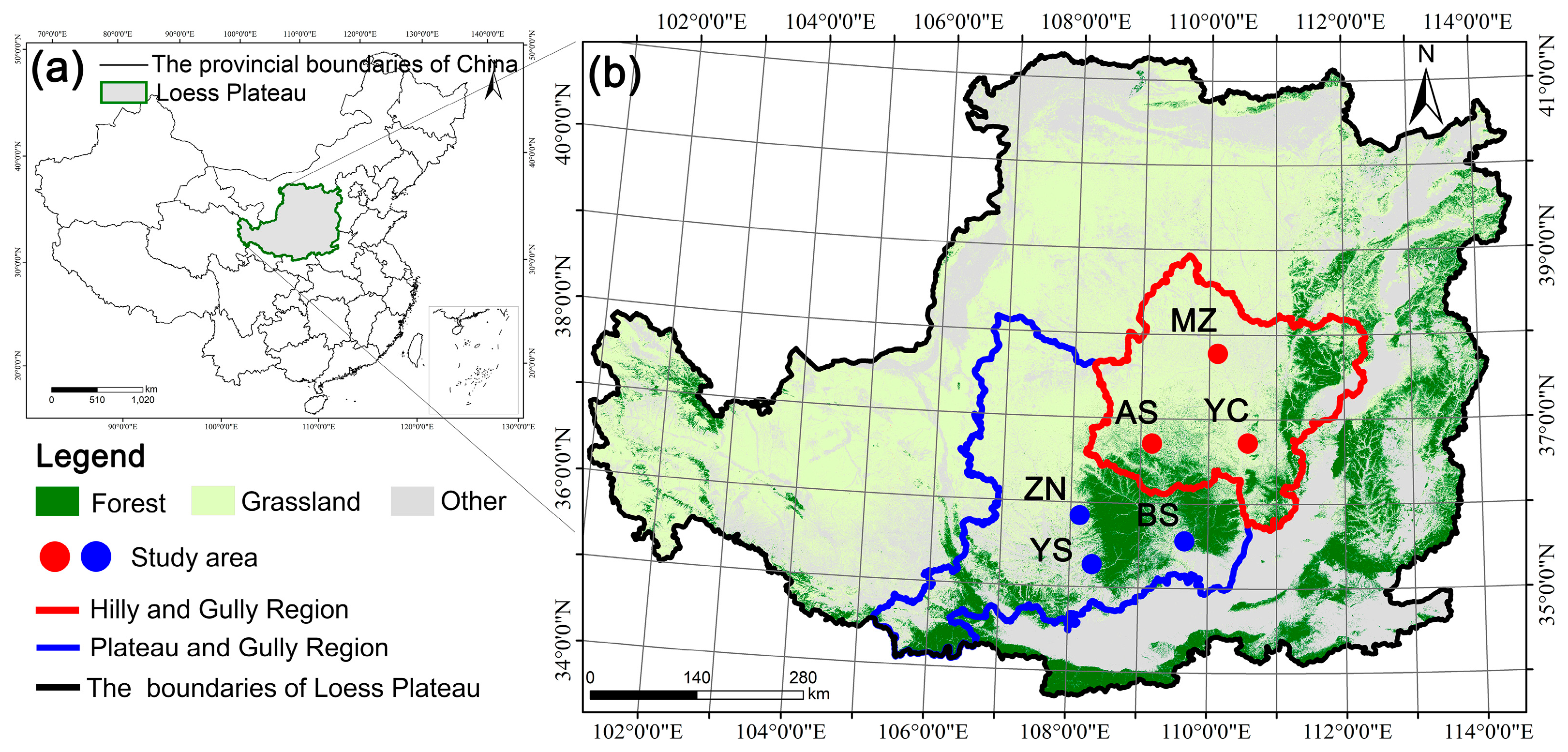
2.1. Study Area and Forest Landscape Data Extraction

The Loess Plateau, located in central and northern China (Figure 1a), is the largest loess distribution area in the world, with a total area of 640,000 km². The region has a temperate semi-arid climate characterized by cold, dry winters and hot summers with concentrated precipitation. Annual precipitation ranges from 500 to 615 mm, decreasing from southeast to northwest, with most of the precipitation occurring from July to September each year [22]. The Loess Plateau features a complex topography characterized by an intricate network of gullies. The main landforms are the plateau gully region, which is relatively flat with deeper and wider gorges and is typically dominated by plateaus, ridges, and mounds, and the hilly gully region, which features a rugged terrain with intricate networks of gorges and is commonly characterized by ridges, mounds, and valleys [23]. This study focuses on six counties: Yongshou (YS), Zhengning (ZN), and Baishui (BS) from the plateau gully region, and Ansai (AS), Mizhi (MZ), and Yanchang (YC) from the hilly gully region. The geographical locations of these counties are shown in Figure 1b.

For the extraction of forest landscape data, this study adheres to the “Land Use Current Status Classification” standard [24] and uses Landsat TM 5/8 (30 m spatial resolution) image data to classify images from 2000, 2010, and 2022 (Table S1). Classification was performed using an object-oriented multi-scale segmentation algorithm, with image segmentation performed using e-Cognition 9.0 software [25].

The classification rule set was established through manual interpretation, including landscape types such as forest, other forest, grassland, cropland, orchard, construction, and water. The Support Vector Machine (SVM) classification algorithm was then applied to train the sample datasets, thereby extracting the primary landscape types of the study area for different time periods (Figure S1). The classification results were evaluated based on the overall accuracy and kappa coefficient, and the classification accuracy met the requirements of the study (Table S2).

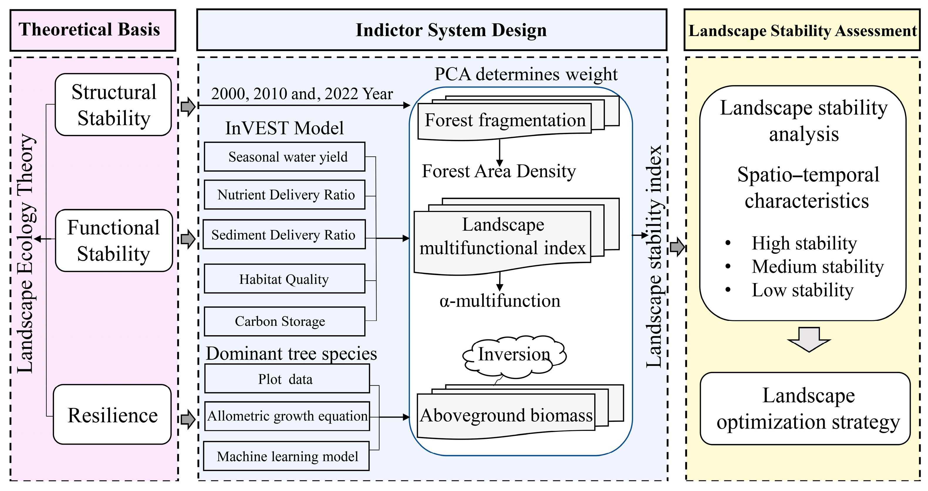
2.2. Forest Landscape Stability Assessment Framework

Based on landscape ecology theory, this study develops a framework for the assessment of forest landscape stability for the Loess Plateau (Figure 2), focusing on three dimensions: structural stability, functional stability, and resilience. The aim is to quantify forest landscape stability and propose appropriate optimization strategies.

Structural stability, as a foundational aspect of landscape stability, reflects the composition and spatial configuration of the landscape. Since forest fragmentation directly reflects the integrity and connectivity of landscape patterns and significantly influences biodiversity conservation and ecological processes [26], it is established as a core indicator for assessing structural stability. Quantifying the degree of forest fragmentation allows an effective assessment of the structural stability of the landscape and its sensitivity to external disturbances, thus revealing its vulnerability and potential risks.

Functional stability is a core dimension in assessing landscape stability, focusing primarily on the integrated capacity of forest ecosystems to provide services. In this study, key ecosystem services in the study area are assessed and functional stability is quantified using Simpson’s Diversity Index (SDI) [27]. The level of the SDI not only reflects the stability of the forest landscape in terms of multifunctionality but also reveals differences in functional contributions between different landscape configurations.

Resilience is a key dimension in assessing landscape stability, indicating the ability of the landscape to recover from external disturbances such as natural disasters and human activities. The vegetation ecological restoration programs in the Loess Plateau (the Grain-for-Green Program and the Natural Forest Protection Program) had a significant impact on above ground biomass (AGB) of forests. AGB, as an important indicator of ecosystem health, reflects both the carbon storage capacity and growth condition of forests, while also indirectly measuring their ability to resist disturbance and restore ecological functions [28]. Therefore, this study selects AGB as the key quantitative indicator of resilience and uses a combination of remote sensing data and ground surveys for its estimation and analysis.

To quantitatively assess the overall stability of forest landscapes on the Loess Plateau, this study introduces the Landscape Stability Index (LSI), which integrates the three dimensions. To capture spatio–temporal variation in the relative importance of stability dimensions, principal component analysis (PCA) was used to dynamically derive dimension-specific weights (W_FAD, W_SDI, W_AGB) for each study area and time period. This method accounts for the varying contributions of structural integrity, functional diversity, and resilience to overall stability across different geomorphic regions and ecological management regimes. Min-max normalization (Equation (1)) of raw indicators ensures comparability of LSI values across time and regions by scaling all components to a [0, 1] range before weighted summation.

PCA is used to determine the weights of the indicators for each dimension (Table 1). The formula for calculating the LSI is as follows:

$$LSI=W_{FAD}·{\displaystyle \frac{{FAD}_i-{FAD}_{imin}}{{FAD}_{imax}-{FAD}_{imin}}}+W_{SDI}·{\displaystyle \frac{{SDI}_i-{SDI}_{imin}}{{SDI}_{imax}-{SDI}_{imin}}}+W_{AGB}·{\displaystyle \frac{{AGB}_i-{AGB}_{imin}}{{AGB}_{imax}-{AGB}_{imin}}}$$

(1)

In the formula, W_FAD, W_SDI, and W_AGB are the weights for forest fragmentation, SDI, and AGB, respectively. FAD, SDI, and AGB are the core indicators of structural stability, functional stability, and resilience, respectively. Here, i represents the individual grid cell, and min and max denote the minimum and maximum values for each indicator.

Table 1. Weight of each dimension indicator.

County	Year	w1	w2	w3
AS	2000	0.883	0.398	0.165
	2010	0.798	0.431	0.283
	2022	0.592	0.482	0.494
MZ	2000	0.645	0.556	0.42
	2010	0.565	0.449	0.441
	2022	0.574	0.46	0.459
YC	2000	0.607	0.468	0.464
	2010	0.792	0.494	0.294
	2022	0.787	0.546	0.179
YS	2000	0.723	0.416	0.335
	2010	0.733	0.422	0.274
	2022	0.707	0.374	0.303
ZN	2000	0.908	0.396	0.171
	2010	0.949	0.382	0.107
	2022	0.801	0.365	0.165
BS	2000	0.805	0.476	0.354
	2010	0.879	0.4	0.194
	2022	0.804	0.411	0.216

Table 1. Weight of each dimension indicator.

County	Year	w1	w2	w3
AS	2000	0.883	0.398	0.165
	2010	0.798	0.431	0.283
	2022	0.592	0.482	0.494
MZ	2000	0.645	0.556	0.42
	2010	0.565	0.449	0.441
	2022	0.574	0.46	0.459
YC	2000	0.607	0.468	0.464
	2010	0.792	0.494	0.294
	2022	0.787	0.546	0.179
YS	2000	0.723	0.416	0.335
	2010	0.733	0.422	0.274
	2022	0.707	0.374	0.303
ZN	2000	0.908	0.396	0.171
	2010	0.949	0.382	0.107
	2022	0.801	0.365	0.165
BS	2000	0.805	0.476	0.354
	2010	0.879	0.4	0.194
	2022	0.804	0.411	0.216

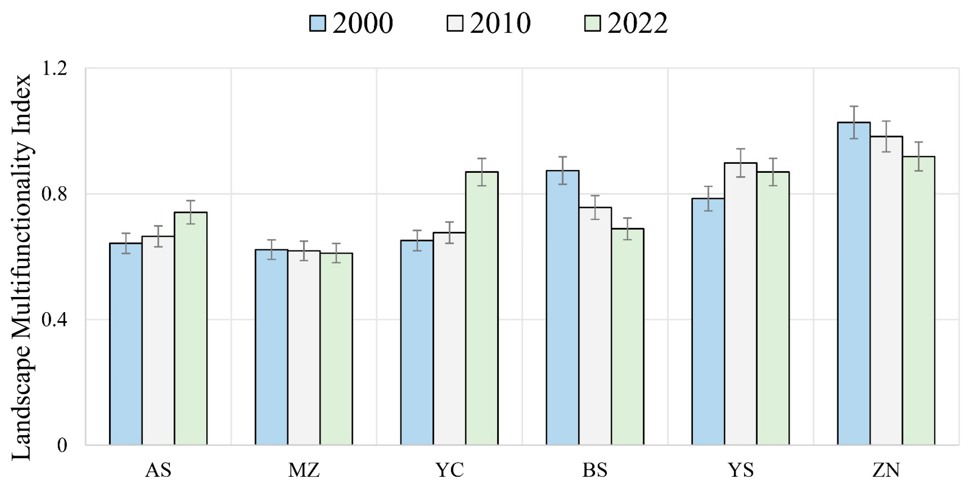
2.3. Multifunctionality of Forest Landscape

2.3.1. Assessment of Key Ecosystem Services

To assess key ecosystem services in the study area, including seasonal water yield (SWY), nutrient delivery ratio (NDR), sediment delivery ratio (SDR), habitat quality (HBQ), and carbon storage (CS), this study employs five modules of the InVEST model developed by Stanford University, WWF, and The Nature Conservancy: SWY, NDR, SDR, HBQ, and CS. The input data and sources for each module are detailed in Table S3.

The SWY module uses local recharge as an indicator of source water conservation, with CN and Kc values provided in Table S4. The biophysical parameter table of the NDR module (Table S5) follows the InVEST model user manual and the relevant literature [29]. For the SDR module, R values are calculated based on average annual and monthly precipitation using the method outlined by [30], while the slope length factor is derived from the methods of [31,32]. P- and C-factor values for the Loess Plateau region are based on studies by [33,34,35,36] (Tables S6 and S7). The HBQ module uses threat and habitat sensitivity factors (Tables S8 and S9) based on studies specific to the Loess Plateau [37,38,39] and the InVEST user manual. The CS module includes parameters for carbon storage components based on the literature and data from the Loess Plateau [40,41,42,43] (Table S10).

The model results were validated by comparison with available data from similar regions of the Loess Plateau. SWY was compared with data from the provincial water resources bulletin (http://slt.shaanxi.gov.cn/; https://shuiwuju.zgqingyang.gov.cn/, accessed on 1 March 2024), while SDR, NDR, HBQ, and CS were compared with results from the related literature [9,44,45] to assess the reasonableness of the simulation results.

2.3.2. Simpson’s Diversity Index

The SDI is widely used to assess the diversity of ecosystem service functions, capturing both their richness and evenness [46]. In this study, the Gini–Simpson diversity index is applied to assess the stability of five ecosystem services at the landscape scale, using a resolution of 30 m pixel. The formula for the SDI is

$$SDI=1-{\sum }_{i=1}^N{p}_i^2$$

(2)

where N is the value of ecosystem service functions, and $p_i^2$ is the proportion of the supply of the ith ecosystem service within a patch relative to the total ecosystem service supply in that patch.

SDI values range from 0 to 1, with higher values indicating greater diversity in ecosystem service provision [27]. The Gini–Simpson diversity index for the five aggregated ecosystem services is computed using the diversity functions in the “vegan” package [47] in R, yielding the SDI distribution for each raster unit.

2.4. Forest Fragmentation

Forest Area Density (FAD) is a critical indicator for assessing forest fragmentation and identifying highly fragmented hotspot areas [48,49]. In this study, the forest classification map is used as a binary input: missing values are assigned 0, background pixels (non-forest areas) are assigned 1, and forest pixels are assigned 2. FAD values are then calculated using a moving window analysis, where the proportion of forest pixels within the window is computed for each foreground pixel and assigned to the corresponding location in the output map.

Due to the scale-dependent nature of the FAD values, this study adopts the observational scale suggested in the previous study to improve assessment accuracy [19]. The FAD results are classified into five fragmentation levels using the classification scheme provided by GuidosToolbox 3.3 (GTB) [50]. These levels are color-coded to visually represent the degree of forest fragmentation. FAD values are divided into the following categories: “Rare” (FAD < 10%), “Patchy” (10% ≤ FAD < 40%), “Transitional” (40% ≤ FAD < 60%), “Dominant” (60% ≤ FAD < 90%), and “Interior” (90% ≤ FAD < 100%). “Rare” indicates highly fragmented areas, while “Interior” represents areas with greater continuity and lower fragmentation.

2.5. Forest Landscape Aboveground Biomass Inversion

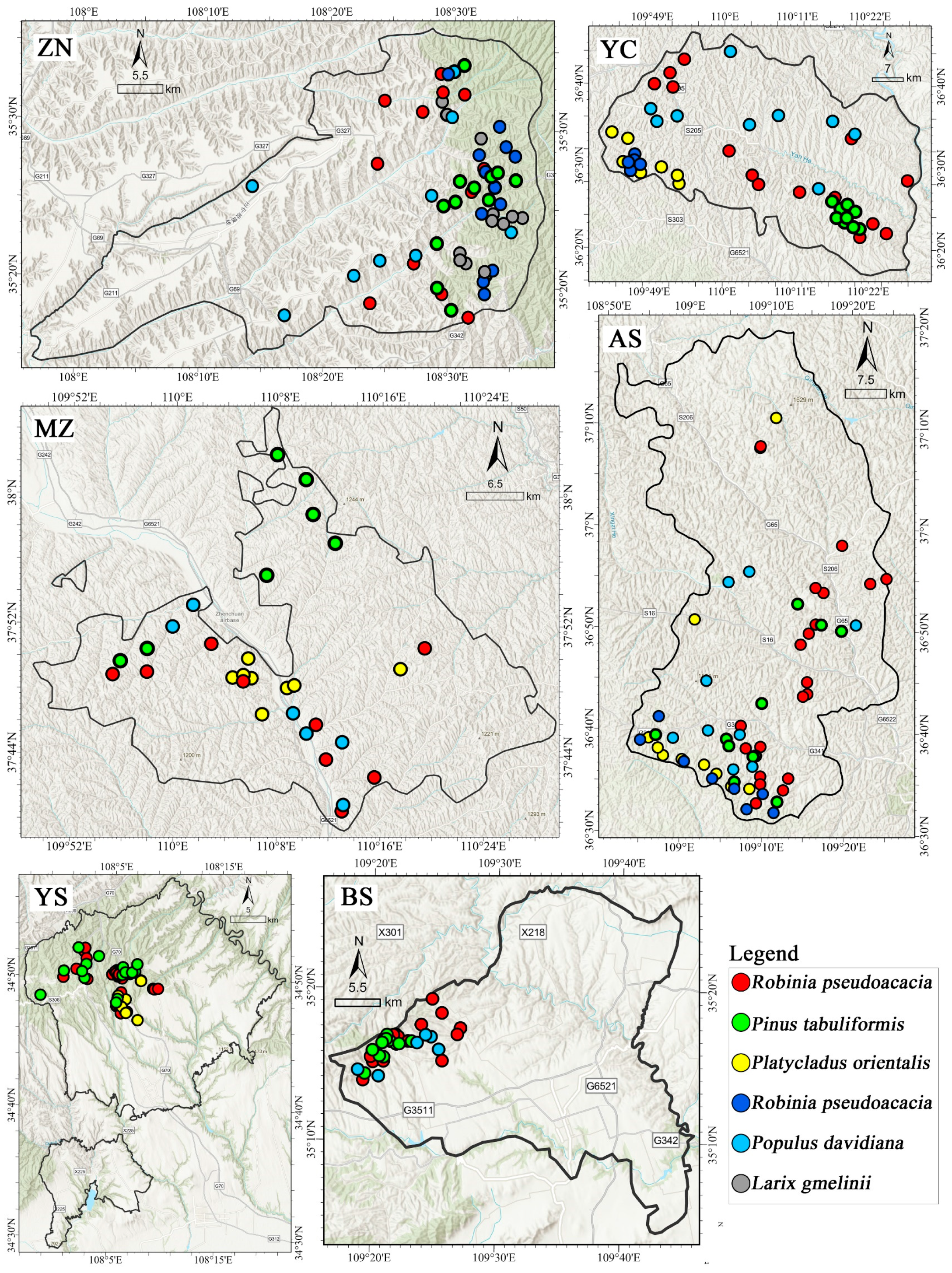
2.5.1. Plot Survey and Biomass Calculation

This study is based on data from the Second National Forest Resources Inventory. From June to August 2022, 295 sample plots were established in six districts of the study area. The plots contained mainly dominant tree species, including Robinia pseudoacacia, Pinus tabuliformis, Platycladus orientalis, Populus davidiana, Quercus mongolica, and Larix gmelinii. Each plot had an area of 30 × 30 m and was distributed as evenly as possible over the study area, with the specific spatial distribution shown in Figure 3. Basic information of the sample plots is provided in

Table 2. Statistical table of basic information of survey sample data in the study area.

County	Species	Quantity	Tree Hight (m)		DBH (cm)
			Average	Range	Average	Range
YS	Robinia pseudoacacia	41	11.78 ± 2.62	5.06–15.97	12.53 ± 5.07	6.18–26.89
	Pinus tabuliformis	16	11.40 ± 2.41	7.27–13.62	16.90 ± 3.25	10.02–22.72
	Platycladus orientalis	11	5.55 ± 1.20	3.50–9.58	7.04 ± 1.69	3.75–9.58
BS	Robinia pseudoacacia	17	10.48 ± 5.25	7.76–11.66	11.84 ± 1.53	6.57–19.56
	Pinus tabuliformis	11	10.92 ± 2.45	6.75–12.56	11.64 ± 1.55	9.56–12.01
	Populus alba	6	7.78 ± 4.23	8.52–9.52	10.10 ± 2.35	7.27–12.74
ZN	Robinia pseudoacacia	18	11.26 ± 1.51	6.48–12.14	10.65 ± 3.26	8.35–15.87
	Quercus mongolica	12	10.29 ± 2.66	8.73–11.94	9.87 ± 1.19	9.17–11.10
	Pinus tabuliformis	14	12.00 ± 2.96	7.95–16.41	15.18 ± 5.37	9.35–15.75
	Populus alba	9	7.92 ± 1.01	6.45–8.15	11.30 ± 0.57	9.15–14.25
	Larix gmelinii	11	16.42 ± 1.25	7.9–22.3	19.01 ± 2.64	6.5–28.6
AS	Robinia pseudoacacia	21	10.24 ± 2.52	5.3–13.8	10.57 ± 2.65	6.77–28.64
	Populus alba	9	8.56 ± 1.45	7.01–11.08	13.94 ± 3.46	9.29–26.45
	Platycladus orientalis	10	6.89 ± 1.89	5.28–8.64	12.09 ± 0.78	7.95–21.65
	Quercus mongolica	8	9.86 ± 5.17	7.89–12.56	12.06 ± 0.76	9.65–19.54
	Pinus tabuliformis	11	11.06 ± 3.45	7.56–13.52	11.99 ± 0.34	9.33–11.98
YC	Robinia pseudoacacia	13	10.21 ± 5.12	7.44–12.34	9.04 ± 1.48	5.99–24.58
	Platycladus orientalis	8	6.32 ± 2.53	5.66–8.19	11.46 ± 3.14	6.29–24.71
	Populus alba	9	8.49 ± 3.42	6.58–10.68	11.71 ± 2.90	6.99–36.75
	Pinus tabuliformis	9	10.77 ± 1.23	6.58–12.37	7.92 ± 1.45	6.68–13.65
	Quercus mongolica	5	9.15 ± 4.75	7.56–10.11	11.66 ± 2.97	7.89–35.95
MZ	Platycladus orientalis	8	9.74 ± 1.92	7.06–12.88	9.36 ± 1.29	6.25–13.25
	Robinia pseudoacacia	9	10.03 ± 2.56	6.28–11.01	10.70 ± 3.84	6.54–17.56
	Pinus tabuliformis	7	9.97 ± 3.02	7.77–11.09	9.46 ± 2.50	6.01–13.59
	Populus alba	6	10.86 ± 4.07	7.98–12.52	15.30 ± 3.04	6.98–18.01

.

The center positions of the plots were recorded using a global positioning system (MG838 GPS) with a positioning accuracy better than 1 m. During the field survey, all trees were individually measured, and the height and diameter at breast height of each tree were recorded. Based on these data, biomass was estimated using allometric growth models applicable to the dominant tree species. The specific calculation methods refer to the models proposed by [51,52] (

Table 3. Allometry model for estimating biomass of dominant tree species.

Species	Allometric Relationships	R2
Robinia pseudoacacia	$B_{trunk}=0.0347{\left({DBH}^{2}H\right)}^{0.921}$	0.980
	$B_{bark}=0.01867{\left({DBH}^{2}H\right)}^{0.7842}$	0.974
	$B_{branch}=0.006173{\left({DBH}^{2}H\right)}^{0.9807}$	0.950
	$B_{leaf}=0.001258{\left({DBH}^{2}H\right)}^{1.0534}$	0.880
Pinus tabuliformis	$B_{bark}=0.37583{DBH}^{-0.51440}{H}^{0.27033}$	0.912
	$B_{branch}=1.17627{DBH}^{0.54089}{H}^{-1.00212}$	0.925
	$B_{leaf}=1.93626{DBH}^{0.19371}{H}^{-1.13112}$	0.952
Quercus mongolica	$B=0.{07509DBH}^{2.32637}{H}^{0.33015}$	0.948
Populus alba	$B=0.04607{DBH}^{2.14892}{H}^{0.59163}$	0.951
Platycladus orientalis	$B=0.08947{DBH}^{1.91489}{H}^{0.61516}$	0.903
Larix gmelinii	$B=0.05851{DBH}^{2.01549}{H}^{0.59146}$	0.961

).

2.5.2. Variable Extraction and Boruta Selection

Spectral information and texture features are key attributes of remote sensing images. In this study, 160 remote sensing variables were selected for forest AGB inversion, including 6 spectral bands, 3 topographic variables, 7 vegetation indices, and 144 texture variables (

Table 4. Remote sensing variables and topographic variables extracted from Landsat images and DEM.

Classes	Variables and Calculation Formulas
Original band	Blue, Green, Red, Nir, SWIR1, SWIR2
Vegetation index	$\mathrm{DVI}=\mathrm{NIR}-\mathrm{R}$
	$\mathrm{EVI}=\mathrm{G}{\displaystyle \frac{\mathrm{NIR}-\mathrm{R}}{\mathrm{NIR}+{\mathrm{C}}_1\mathrm{R} - {\mathrm{C}}_2\mathrm{B}+\mathrm{L}}}$
	$\mathrm{MSAVI}={\displaystyle \frac{2\mathrm{NIR}+1 - \sqrt{{\left(2\mathrm{NIR}+1\right)}^2 - 8\left(\mathrm{NIR}-\mathrm{R}\right)}}{2}}$
	$\mathrm{NDVI}={\displaystyle \frac{\mathrm{NIR} - \mathrm{R}}{\mathrm{NIR}+\mathrm{R}}}$
	$\mathrm{NLI}={\displaystyle \frac{{\mathrm{NIR}}^2 - \mathrm{R}}{{\mathrm{NIR}}^2+\mathrm{R}}}$
	$\mathrm{SAVI}=\left(1+\mathrm{L}\right){\displaystyle \frac{\mathrm{NIR} - \mathrm{R}}{\mathrm{NIR}+\mathrm{R}+\mathrm{L}}}$
	$\mathrm{S}\mathrm{R}=\mathrm{N}\mathrm{I}\mathrm{R}/\mathrm{R}$
Texture variable	Angular second moment (ST), Contrast (CT), Correlation (CN), Dissimilarity (DY), Entropy (EY), Homogeneity (HY), Mean (MN), Variance (VE)
Topographic variables	Elevation, Aspect, Slope

γ represents the proportion of the blue wave segment reflectance in ARVI, where γ = 1. The atmospheric correction parameters C₁ and C₂ are 6.0 and 7.5, respectively. The value of parameter L is 1.0 in EVI and 0.5 in SAVI.

). Texture feature extraction was primarily based on the gray-level co-occurrence matrix (GLCM) method, and 8 s-order GLCM features were selected for analysis. Window sizes of 3 × 3 and 5 × 5 were used for texture calculation, and all calculations and variable extraction were performed using ENVI 5.3 software.

2.5.3. Machine Learning Models and Performance Evaluation

Three commonly used machine learning methods were employed to invert the AGB of the study area: Random Forest (RF), SVM, and eXtreme Gradient Boosting (XGBoost). These methods are widely used in remote sensing and ecological data analysis due to their advantages in handling nonlinear relationships, high-dimensional features, and improving prediction accuracy.

RF is an ensemble learning method based on decision trees, where multiple decision trees are constructed and combined using a voting mechanism for prediction. This method has strong resistance to overfitting and high prediction accuracy. In this study, the RF model used key variables selected by the Boruta method as input features, with 30 trees (ntree = 30), and modeling was conducted on the training data set, followed by prediction on the test set.

SVM is a supervised learning algorithm based on statistical learning theory, which is particularly suitable for small sample and nonlinear problems. In this study, the SVM model used the Radial Basis Function kernel, which optimizes the support vectors in the training data to construct a predictive model. The flexibility of the model enables it to effectively capture complex variable relationships and make predictions on the test set.

XGBoost is a decision tree model based on the gradient boosting framework, which is known for its efficient training speed and powerful feature representation ability [53]. In this study, the XGBoost model used squared error (reg: squarederror) as the objective function, with a learning rate (eta = 0.1) and a maximum depth (max_depth = 6), and iterated for 100 optimization rounds on the training set, ultimately predicting the test set.

Model performance was evaluated using three metrics: R², root mean square error (RMSE), and relative root mean square error (rRMSE). R² reflects the ability of the model to explain the data, while RMSE and rRMSE measure the deviation between the predicted and observed values. Ultimately, the optimal model for AGB inversion was determined by comparing the performance metrics of the three models.

3. Results

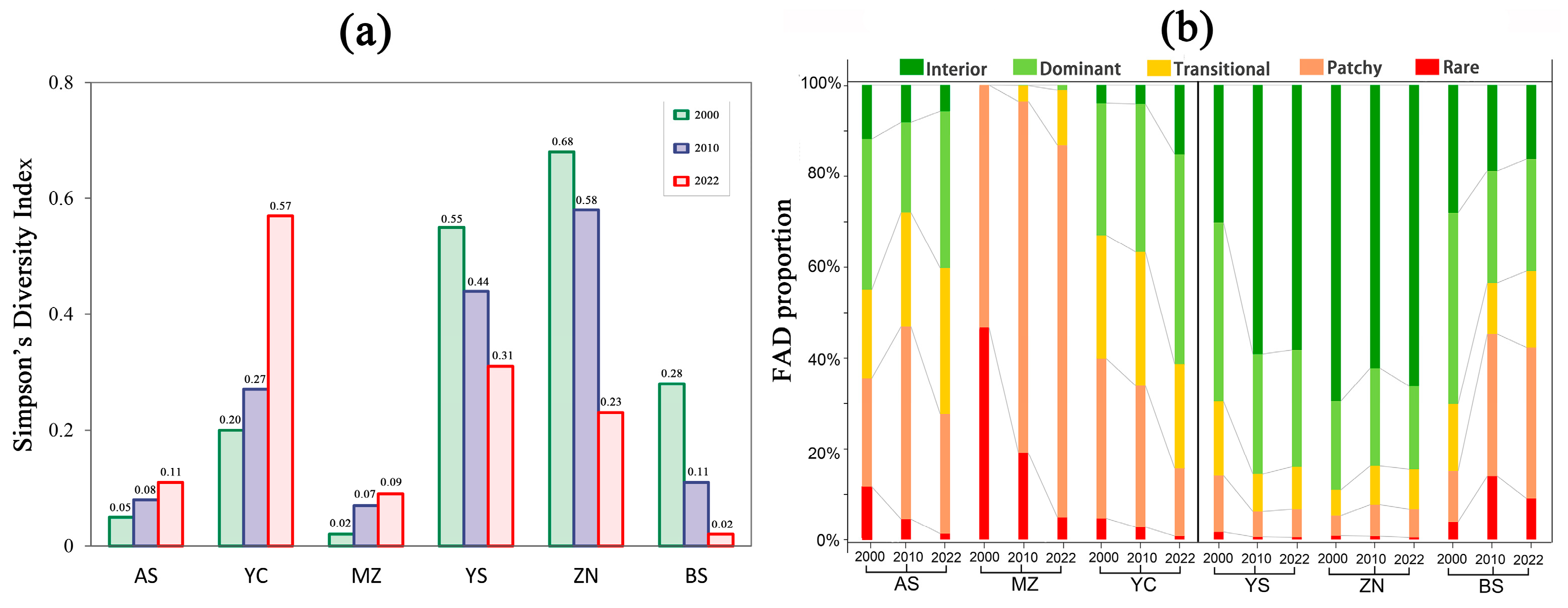
3.1. Forest Landscape SDI and Forest Fragmentation Characteristics

As shown in Figure 4a, there were significant differences in the SDI of various counties in 2000, 2010, and 2022. In the hilly gully region, the SDI of AS gradually increased from 0.05 in 2000 to 0.11 in 2022, exhibiting a clear upward trend, indicating an improvement in forest landscape stability. The SDI of YC increased significantly from 0.20 in 2000 to 0.57 in 2022, showing the highest growth of multifunctionality. The SDI of MZ also showed an upward trend, rising from 0.02 in 2000 to 0.09 in 2022. Although the increase was relatively small, it still reflected a gradual improvement in the stability of the forest landscape. In contrast, in the plateau gully region, the SDI of the three counties exhibited a decreasing trend over time. The SDI of ZN decreased from 0.68 in 2000 to 0.58 in 2010, and further decreased sharply to 0.23 in 2022, indicating a drastic decline in forest landscape stability. The SDI of YS decreased slightly from 0.55 to 0.44 from 2000 to 2010, followed by a significant decline to 0.31 in 2022. The SDI of BS decreased from 0.28 to 0.11 from 2000 to 2010, with a further decrease to 0.02 in 2022.

As shown in Figure 4b, the degree of forest fragmentation was generally higher in the hilly gully region than in the plateau gully region. In the plateau gully region, although the fragmentation degree showed a slight downward trend, YS and ZN were dominated by low fragmentation types such as “Interior” and “Dominant”. The proportions of various fragmentation types in BS were relatively even, indicating that the overall fragmentation degree was higher than in YS and ZN. The forest fragmentation degree in the hilly gully region was higher, with MZ having the highest fragmentation level, mainly consisting of “Patchy” and “Rare” types, which accounted for more than 80%. Compared to the plateau gully region, the hilly gully region showed a more pronounced decrease in overall fragmentation, with significant improvements in MZ and YC. In summary, the hilly gully region exhibited greater dynamics, with substantial changes between fragmentation types. In contrast, the plateau gully region showed greater stability, with “Interior” and “Dominant” types maintaining dominance, although there was a slight shift towards “Patchy” and “Transitional” types.

3.2. Forest Landscape AGB Inversion

3.2.1. AGB Estimation Explanatory Variables and Their Importance

As shown in Figure 5a,b, a total of 26 important variables were selected through the Boruta algorithm, covering visible light bands (R, G, B), short-wave infrared bands (SWIR1, SWIR2), topographic factors (DEM), and various texture features extracted using the GLCM. These variables contributed significantly to the AGB estimation, with their importance ranking shown in Figure 5c. Among them, DEM and SWIR1 exhibited the highest importance, indicating that topographic and spectral information have a significant impact on the spatial distribution of AGB. The B band in the visible light spectrum and the SWIR2 band in the short-wave infrared also showed high importance, reflecting the sensitivity of vegetation to the reflective properties of different bands. The texture feature variables extracted using GLCM, such as R3_MN, G7_VE, R7_EY, and R7_ST, played a key role in capturing spatial heterogeneity and AGB distribution.

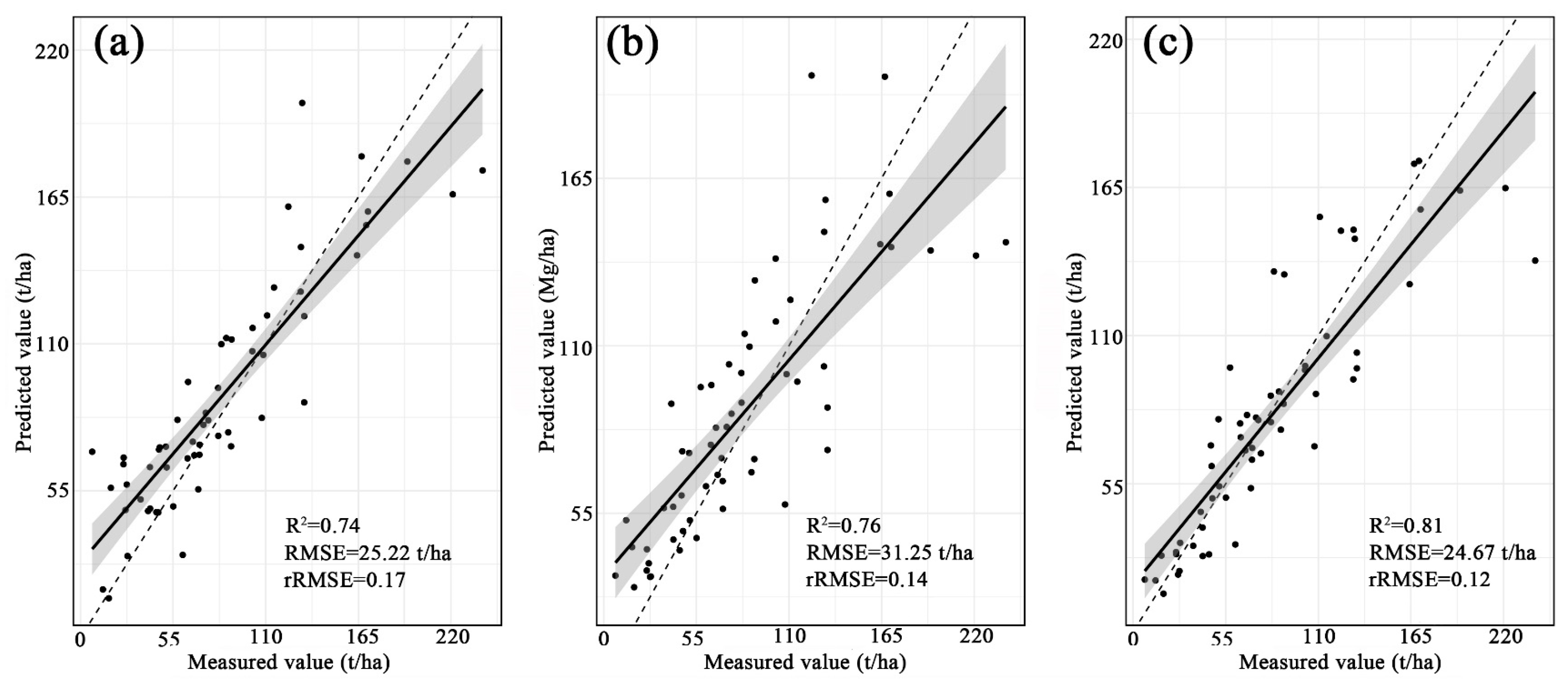
3.2.2. Validation of AGB Estimation Accuracy

In this study, a comparative analysis of AGB estimation performance was conducted using three models, SVM, RF, and XGBoost, whose predictive abilities were validated based on measured data. As shown in Figure 6, the results demonstrate that all three models effectively estimate AGB, though with significant differences in performance. The SVM model had an R² of 0.74, an RMSE of 25.22 ton ha⁻¹, and an rRMSE of 0.17, showing relatively weak performance (Figure 6a). The RF model outperformed the SVM with an R² of 0.76, an RMSE of 31.25 ton ha⁻¹, and an rRMSE of 0.14, demonstrating stronger robustness (Figure 6b). The XGBoost model achieved the highest prediction accuracy with an R² of 0.81, an RMSE of 24.67 ton ha⁻¹, and an rRMSE of 0.12, showing superior nonlinear modeling capability and adaptability (Figure 6c). The overall analysis indicates that the XGBoost model has a significant advantage in AGB estimation, and therefore it was selected for the AGB inversion of the forest landscape in the study area.

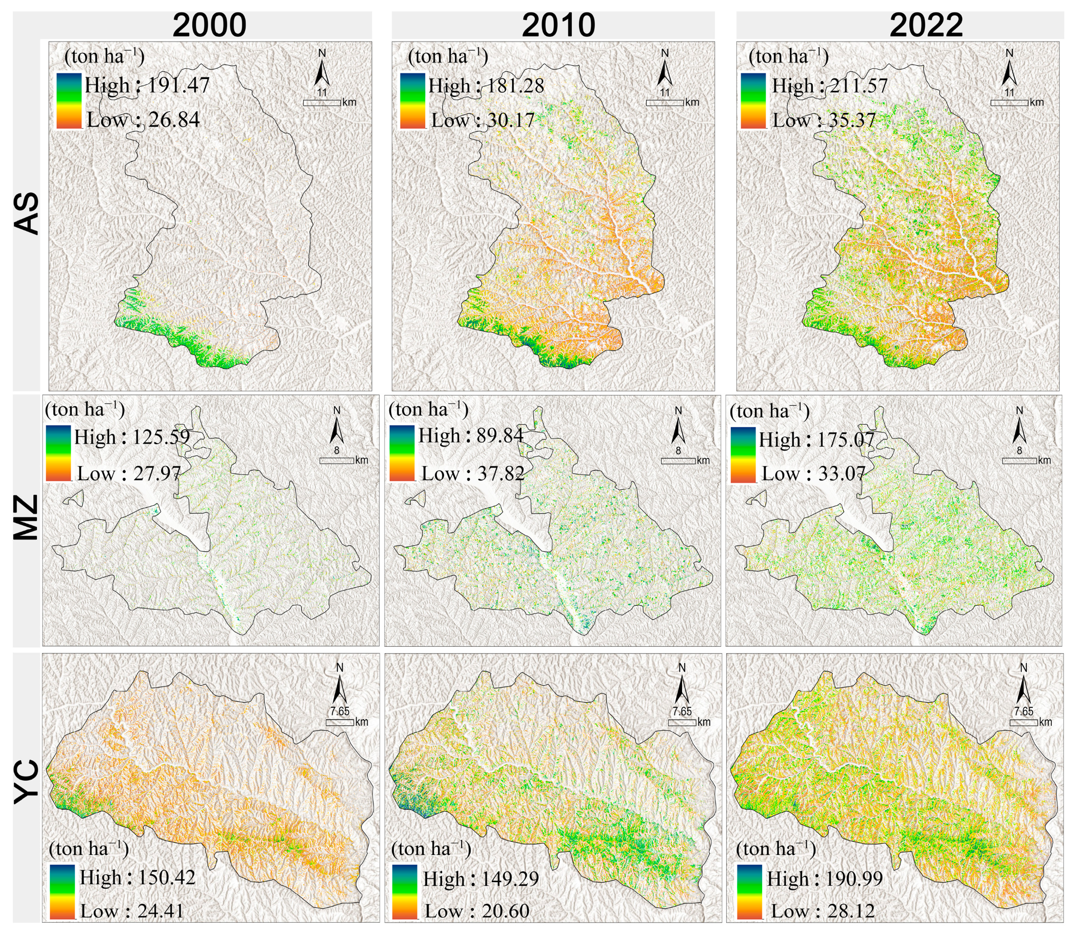
3.2.3. Spatio–Temporal Dynamics of AGB

As shown in

Table 5. Aboveground biomass was estimated in 2000, 2010, and 2022 in the study area (ton ha⁻¹).

Year	AS	MZ	YC	BS	YS	ZN
2000	93.07	65.75	44.52	61.00	85.61	104.88
2010	64.36	67.07	45.16	62.13	70.75	99.45
2022	95.13	88.88	80.48	78.48	82.86	118.75

, from 2000 to 2010, AGB decreased in the hilly gully region, with AS’s AGB decreasing from 93.07 tons ha⁻¹ to 64.36 tons ha⁻¹. Between 2010 and 2022, AGB increased in all counties in the hilly gully region, with the AGB of AS recovering to 95.13 tons ha⁻¹, approaching the 2000 level. Biomass in MZ and YC also increased to 88.88 tons ha⁻¹ and 80.48 tons ha⁻¹, respectively. In contrast, changes in AGB in the plateau gully region were relatively stable. Between 2000 and 2010, AGB in BS decreased slightly to 62.13 tons ha⁻¹, before rising to 78.48 tons ha⁻¹ by 2022. In 2022, AGB in YS reached 82.86 tons ha⁻¹, while AGB in ZN increased to 118.75 tons ha⁻¹, showing a continuous increase since 2000.

Significant differences in AGB were observed across time periods and regions of the study area for 2000, 2010, and 2022. In the plateau gully region, the spatial distribution of AGB in YS and BS counties exhibited a southeast-to-northwest gradient, with lower values in the southeast and higher values in the northwest. The high AGB areas in ZN were primarily concentrated in the eastern part (Figure 7). In the hilly gully region, the spatial distribution of AGB was more dispersed. Between 2000 and 2022, AS and YC counties showed a concentrated distribution in the southern part and gradually dispersed northward. The spatial distribution of AGB in MZ was the most dispersed (Figure 8).

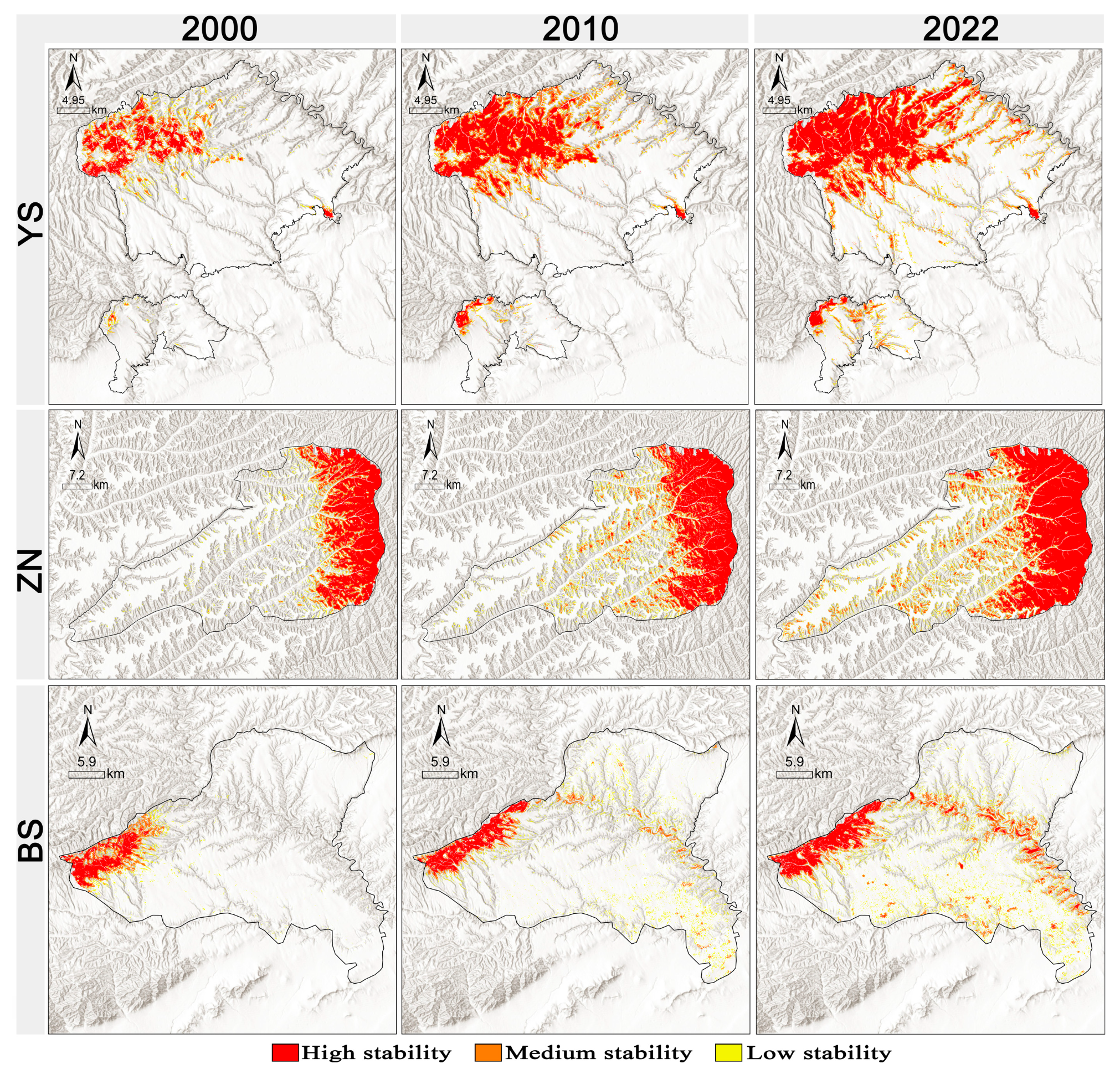
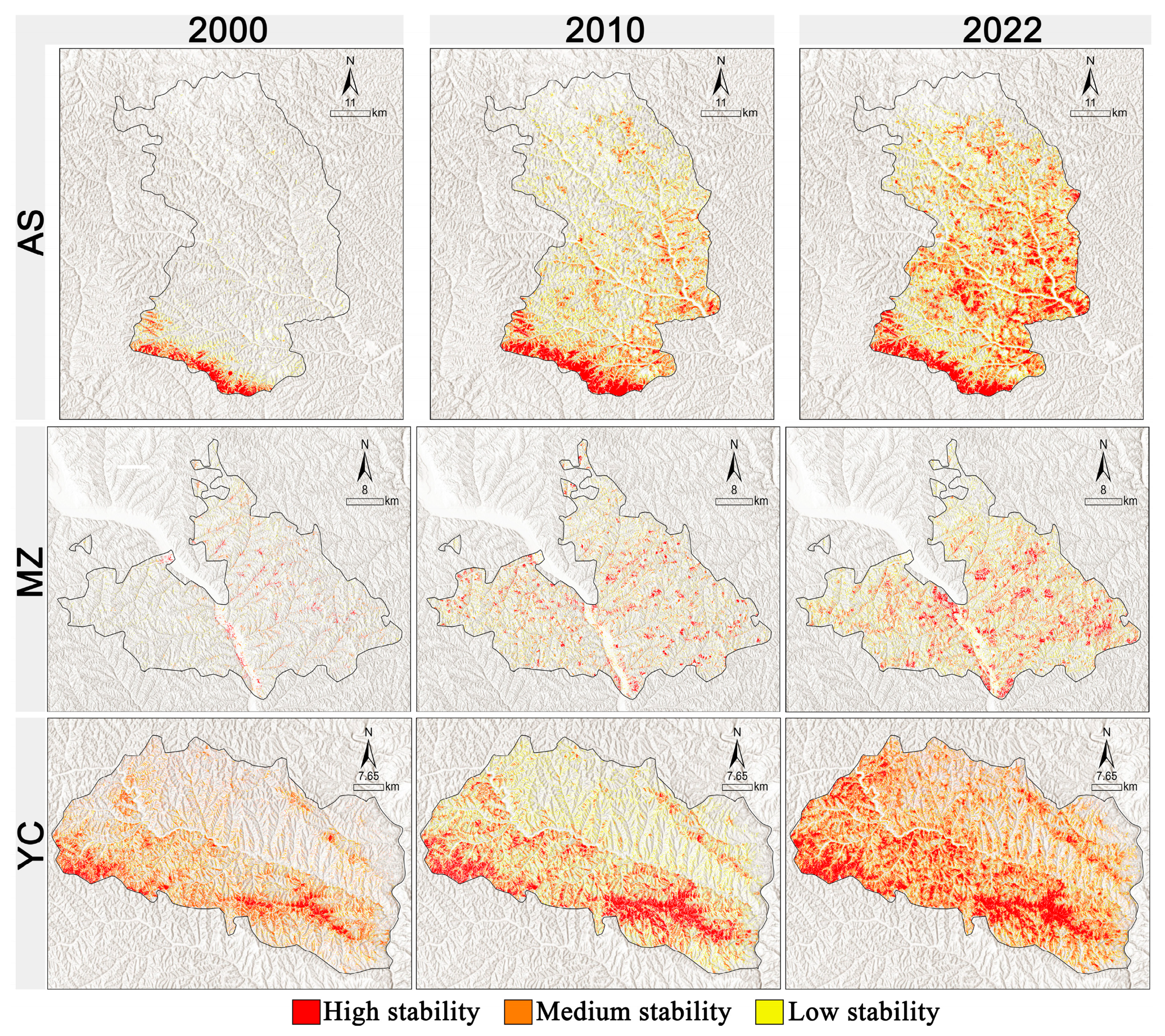
3.3. Spatial Distribution Pattern of the Forest Landscape Stability Index

Figure 9 illustrates the spatio–temporal changes of the forest LSI in the study area for the years 2000, 2010, and 2022, highlighting significant variations among counties. In the hilly gully region, the LSI generally shows an upward trend, except in MZ. In AS, the LSI increased from 0.64 in 2000 to 0.74 in 2022, reflecting a notable enhancement in landscape stability. YC saw the largest increase in the region, with the LSI rising from 0.65 in 2000 to 0.86 in 2022, indicating substantial improvement in ecological stability. The LSI of MZ remained relatively stable, with a slight decrease from 0.62 in 2000 to 0.61 in 2022, suggesting minimal changes in stability. In contrast, the LSI in the plateau gully region generally decreased, except in YS. The LSI of ZN decreased from 1.02 in 2000 to 0.91 in 2022, indicating a decline in forest landscape stability. BS county’s LSI decreased from 0.87 in 2000 to 0.68 in 2022, marking the largest decrease in the plateau gully region and suggesting a weakening of forest stability. In YS, the LSI peaked at 0.89 in 2010 and declined slightly to 0.86 in 2022, showing relatively little change in stability.

Figure 10 shows the spatial distribution of the forest LSI in the plateau gully region at three different time points. In 2000, high stability areas were primarily located in the northern and eastern parts of YS and ZN counties, with a relatively limited distribution. By 2010, the area of high stability regions had decreased significantly, reflecting lower forest stability. By 2022, however, ecological restoration efforts had resulted in a significant expansion of high stability areas in most counties, particularly in ZN and BS counties, where restoration effects were most evident.

Figure 11 shows the spatial changes in the forest LSI in the hilly gully region. In 2000, areas of high stability were dispersed and concentrated in certain regions. By 2010, low stability areas had increased significantly, indicating a decline in ecological stability. However, in 2022, with the implementation of ecological restoration measures, high stability areas expanded significantly and low stability areas decreased, while forest fragmentation in the region improved (Figure 4b), and the overall ecosystem service function improved (Figure 4a). Especially in YC, high stability areas showed a relatively large increase and expansion, reflecting the good results of ecological restoration in the region.

4. Discussion

This study, grounded in landscape ecology theory, integrates FAD, SDI, and AGB into a forest landscape stability framework for the Loess Plateau from three dimensions: structural stability, functional stability, and resilience. It innovatively proposes the new LSI, which enables policymakers to better identify and assess high-risk areas and propose targeted optimize strategies to enhance forest landscape stability. This work broadens the methodological approach for assessing forest landscape stability in arid and semi-arid regions.

4.1. Characteristics Analysis of FAD, SDI, and AGB

A comprehensive understanding of the dynamic characteristics of structural stability, functional stability, and resilience is essential for assessing forest landscape stability. The degree of forest fragmentation in the hilly gully region is generally higher than that in the plateau gully region, implying that the integrity and connectivity of forest landscapes are better preserved in the plateau gully region. For the SDI, there is significant spatial heterogeneity among counties. BS, AS, and MZ have low SDI values, indicating lower levels of multifunctionality in these areas, where a single ecosystem service function dominates [54]. MZ faces complex land use and climatic conditions, and some areas are still in transition from cropland and wasteland to artificial forests, which have not yet developed a stable forest structure [55]. In BS, land use changes (such as orchard expansion), climate change, and human activities (such as urbanization and infrastructure development) may interact to alter forest landscape structure and pattern, leading to ecological pressure [56]. The overall AGB in the plateau gully region is higher than in the hilly gully region, which is closely related to the ecological conditions (temperature and precipitation) and vegetation restoration objectives specific to each county [57]. Ecological restoration in the hilly gully region is more comprehensive, coupled with soil and water conservation efforts, while the plateau gully region focuses more on vegetation restoration and soil improvement.

As a key indicator of resilience, AGB plays a central role in assessing the resilience of forest landscapes in this study. This study compares different machine learning models integrating remote sensing and plot data to successfully invert forest AGB in the study area. XGBoost performs optimally in AGB estimation (R² = 0.81), which is better than SVM and RF, since XGBoost can efficiently capture complex nonlinear features while reducing overfitting in constructing complex nonlinear models [58]. The 26 key variables identified through the Boruta algorithm provide effective explanatory factors for AGB estimation. Among them, terrain factors (DEM) and short-wave infrared band (SWIR1) emerged as the key predictors of AGB. SWIR1 reflects the reflective properties of vegetation related to water and heat regulation, while terrain affects AGB by influencing the moderating effects of microclimate moisture, and thus AGB accumulation. Ref. [59] also confirms the importance of terrain factors and remotely sensed spectral data for AGB estimation. While texture features extracted using GLCM were critical in capturing spatial heterogeneity, their contribution to biomass estimation was somewhat less significant. In the hilly gully region, AGB showed a positive restoration trend, suggesting that ecological restoration initiatives—such as crop-to-forest conversion and natural forest protection—have significantly enhanced forest ecosystem services and biomass accumulation. These results are consistent with those of [60,61] and support the role of ecological restoration efforts in improving forest ecosystem health and stability.

4.2. Differences in Dynamics of Forest Landscape Stability in Different Geomorphic Types

Forest landscape stability is a key indicator for assessing the health and resilience of forest ecosystems [62]. The weights of FAD, SDI, and AGB required to calculate the forest LSI were obtained by PCA (Table 1). The results show that these three-dimensional indicators exhibit significant spatial and temporal heterogeneity. The weight of FAD is higher than that of SDI, and SDI is higher than AGB, indicating that FAD consistently plays a dominant role in the calculation of the LSI (plateau gully region: 0.707–0.949; hilly gully region: 0.565–0.883). This phenomenon reflects the stability of forest landscape structure, where forest fragmentation is considered a major limiting factor for landscape stability and is highly susceptible to edge effects and biodiversity loss.

Contrasts in the dynamics of landscape stability across geomorphic types highlight the profound impact of landscape constraints on ecological processes. The forest LSI in the hilly gully region showed an overall upward trend, while in the plateau gully region, it showed a downward. This disparity is largely due to the varying geographical and ecological contexts across different landforms, which result in different responses to forest restoration efforts. In the hilly gully region, the terrain is characterized by deep ravines and steep slopes that are highly susceptible to severe soil erosion. However, through a series of restoration measures such as farmland to forest conversion, forest closure, and ecological slope protection, vegetation cover has improved significantly, soil erosion has been mitigated, and vegetation recovery has been substantial. As a result, the stability of the forest landscape in this region has improved [63,64]. In contrast, the plateau gully region has relatively flatter terrain, which has facilitated human activities such as farming, overgrazing, and illegal logging that contribute to increased land degradation [65]. While some ecological restoration measures have been implemented, the slow pace of recovery in this region is primarily due to monoculture forest structures, extended dry spells, and irregular precipitation patterns. These factors have resulted in inadequate water supplies, and overuse of water resources has further compounded the challenges of vegetation recovery, leading to slower progress in ecological restoration [66].

The significant improvement in the forest LSI in YC county (from 0.65 in 2000 to 0.86 in 2022) results from the synergistic optimization of landscape structure, function, and resilience. Structural stability has been strengthened. YC county effectively reduced forest patch fragmentation through large-scale afforestation. The forest fragmentation type has shifted from “Patchy” to “Dominant” and “Interior” (Figure 4b), which is associated with the terracing and ecological corridor construction in the county [67,68]. The reshaping of the terrain (construction of check dams and terracing) has reduced surface runoff cutting through forest areas, thereby enhancing landscape connectivity. Functional stability has significantly improved. The SDI in YC county increased from 0.20 to 0.57 (Figure 4a), reflecting a substantial improvement in ecosystem service diversity. The county adopted multifunctional vegetation configurations (mixed coniferous and broadleaf forests, mixed tree and shrub forests) to optimize tree species structure, enhance forest disease and stress resistance, and maintain biodiversity. After 2010, the AGB in YC county increased from 64.36 to 80.48 ton ha⁻¹ (Table 5), indicating that under vegetation restoration projects, artificial forests (Robinia pseudoacacia) have gradually transitioned from middle-aged forests to mature forests, with peak AGB accumulation [69]. The improvement in stability in YC county is notable, with vegetation restoration effects surpassing those of other regions. Therefore, this model can be adapted and promoted under specific conditions, particularly in the hilly gully region, where terrain fragmentation can be addressed through engineering measures (terracing) to achieve unified management.

4.3. Optimization Strategy for Improving Forest Landscape Stability in Loess Plateau

(1)

Hierarchical management of forest fragmentation

Implement hierarchical management of forest fragmentation hotspots to optimize forest landscape structure. In areas with high fragmentation (FAD < 10%), such as the hilly gully region (where “Rare” and “Patchy” account for over 80% in counties like MZ), a “patch infill-corridor connection” strategy could be implemented [70]. Fast-growing pioneer species (Hippophae rhamnoides) could be planted in highly fragmented patches to quickly form a cover layer. Wide ecological corridors could be established along gully lines to connect isolated patches and promote species migration and gene flow.

In areas of moderate to low fragmentation (e.g., AS county in the plateau gully region), the focus could be on defending against human disturbances. Strictly safeguard ecological protection red lines, prohibiting mining and cultivation on steep slopes. Promote near-natural forestry management, optimizing stand structural stability through methods such as selective logging and nurturing.

(2)

Multi-objective management to improve SDI

In areas with low SDI, identify low ES categories based on ES evaluation results and implement multi-objective management strategies to enhance forest landscape functionality.

In BS county of the plateau gully region (SDI = 0.02), improving the SDI is a key goal. This can be achieved by optimizing vegetation structure. Plant herbaceous species (Medicago sativa) at erosion-prone gully heads to quickly stabilize soil. Adopt a progressive “grass-shrub-tree” restoration approach: initially, herbaceous plants cover the soil to reduce bare ground, followed by introducing shrubs (Caragana korshinskii) to enhance water retention, and eventually planting trees (Pinus tabuliformis) to enhance carbon sequestration.

In areas with degraded ecosystems, particularly those with steep slopes and serious soil erosion, a combined approach using engineering measures (terracing, fish-scale pits) and biological measures (planting deep-rooted plants) could be implemented for restoration [71].

Construct multifunctional forestry. Develop tree species that provide both ecological and economic benefits, such as Juglans regia, Malus pumila, and Zanthoxylum bungeanum. Utilize understory space to develop non-timber forest products such as medicinal herbs, fungi, and poultry to improve land use efficiency.

For YC county (SDI > 0.5), the focus could be on optimizing functional synergies. Establish a “mixed forest-understory economy” model, such as planting medicinal herbs (Astragalus membranaceus) under Pinus tabuliformis, which maintains CS while reducing logging pressure through economic output. Additionally, establish a 50 m wide no-harvest buffer zone along riverbanks to synergistically improve HBQ and SWY.

(3)

AGB-Driven adaptive management to enhance resilience

For the decline in AGB in AS county of the hilly gully region between 2000 and 2010, improve site conditions. Apply biochar to infertile slopes to enhance soil fertility and water retention capacity. Select drought-resistant tree species and use mycorrhizal inoculation techniques to promote seedling survival [72].

For ZN county in the plateau gully region, which has relatively high AGB, it is important to prevent pests, disease, and fire risks. Use UAV remote sensing to monitor forest health and promptly remove dead standing trees. Establish firebreaks along forest edges (width ≥ 30 m) and plant fire-resistant species to reduce the risk of wildfire.

(4)

Integrating landscape stability into land use planning

Based on the spatial distribution of the LSI (Figure 10 and Figure 11), designate high-stability areas as ecological conservation core zones where development is prohibited. In medium-stability areas, promote eco-tourism or non-timber forest products in the understory. In low-stability areas, implement measures such as converting farmland back to forest and facilitating population relocation. Incorporate the LSI into local government performance evaluation systems, set quantifiable targets, and ensure that strategies are practical and implementable.

4.4. Limitations and Prospects

This study enhances the scientific and accurate assessment of forest landscape stability by incorporating key indicators such as SDI and AGB. However, there are still several limitations: First, the lack of dynamic simulations over long time scales, particularly with insufficient attention to the recovery trajectories of slow-growing species; second, socio-economic factors (e.g., grazing pressure and policy compliance) have not been fully incorporated, affecting the effectiveness of integrated management. Future research could integrate model-based approaches, simulating the interactions between humans and nature, and include more socio-economic factors to explore the coupling relationship between ecology and society and promote a win-win scenario for ecological protection and economic development. Additionally, the study area covers only a few counties, and future research could expand the scope to include more landform types, improving the representativeness and generalizability of the results. At the same time, more ground-truth data could be incorporated to verify and improve the assessment results, strengthen the field monitoring of ecosystem service functions, and provide more accurate data support. Higher-resolution remote sensing data (e.g., Sentinel-2) could also improve AGB estimation accuracy. The impacts of climate change (e.g., changes in precipitation patterns) were not sufficiently considered in this study, limiting the ability to predict future ecological trends. Future research could integrate climate models to enhance prediction reliability. This study proposes optimization strategies for enhancing landscape stability, but caution is needed regarding the varying effects of landform types on restoration efforts. A one-size-fits-all policy, such as uniform afforestation targets, may exacerbate instability in ecologically sensitive areas. It is therefore essential to adapt and improve strategies based on local conditions.

5. Conclusions

Based on landscape ecology, this study constructed a framework to assess the stability of forest landscapes of different landform types in the Loess Plateau from three dimensions: structural stability, functional stability, and resilience. By integrating the core indicators of FAD, SDI and AGB, the forest LSI was innovatively proposed to realize the quantitative assessment and spatial–temporal divergence resolution of forest landscape stability in the region.

After the implementation of the ecological restoration project, the LSI of the hilly gully region increased (especially YC county), the synergistic enhancement of landscape fragmentation and ES effectively enhanced the adaptability of the regional ecosystem, and the stability of the forest landscape in this area showed a significant trend of enhancement. In contrast, the ecological restoration effect in the plateau gully region was relatively slow. The AGB inversion model XGBoost (R² = 0.81), constructed based on remote sensing data and ground survey validation, revealed the spatial and temporal evolution of AGB under different landform types between 2000 and 2022, which provided a quantitative method for landscape resilience assessment. Optimization strategies such as fragmentation hierarchy management, multi-objective management ES, and adaptive management to enhance resilience were proposed for the forest landscape stability differentiation characteristics. This study provides a scientific basis for ecological restoration and forest landscape optimization in the Loess Plateau region, as well as practical optimization paths for policymakers to promote sustainable ecological development in the region.

Although this study provides an important framework for assessing forest landscape stability, there are still some limitations, such as the lack of dynamic modeling on long-term time scales and the failure to consider socio-economic factors. Future research could further expand the study area, incorporate more ground-truthing data, improve the assessment system, and integrate the impacts of climate change to improve the accuracy and reliability of predictions.

References

1. Mori, A.S. Ecosystem management based on natural disturbances: Hierarchical context and non-equilibrium paradigm. J. Appl. Ecol. 2011, 48, 280–292. [Google Scholar] [CrossRef]
2. Wu, J.; Loucks, O.L. From Balance of Nature to Hierarchical Patch Dynamics: A Paradigm Shift in Ecology. Q. Rev. Biol. 1995, 70, 439–466. [Google Scholar] [CrossRef]
3. Walker, B.; Salt, D. Resilience Thinking: Sustaining Ecosystems and People in a Changing World; Island Press: Lahaina, HI, USA, 2006. [Google Scholar]
4. Ghazoul, J.; Chazdon, R. Degradation and recovery in changing forest landscapes: A multiscale conceptual framework. Annu. Rev. Environ. Resour. 2017, 42, 161–188. [Google Scholar] [CrossRef]
5. Milad, M.; Schaich, H.; Bürgi, M.; Konold, W. Climate change and nature conservation in Central European forests: A review of consequences, concepts and challenges. For. Ecol. Manag. 2011, 261, 829–843. [Google Scholar] [CrossRef]
6. Seidl, R.; Thom, D.; Kautz, M.; Martin-Benito, D.; Peltoniemi, M.; Vacchiano, G.; Reyer, C.P. Forest disturbances under climate change. Nat. Clim. Change 2017, 7, 624–632. [Google Scholar] [CrossRef]
7. Jiang, C.; Zhang, H.; Wang, X.; Feng, Y.; Labzovskii, L. Challenging the land degradation in China’s Loess Plateau: Benefits, limitations, sustainability, and adaptive strategies of soil and water conservation. Ecol. Eng. 2019, 127, 135–150. [Google Scholar] [CrossRef]
8. Wen, X.; Deng, X. Current soil erosion assessment in the Loess Plateau of China: A mini-review. J. Clean. Prod. 2020, 276, 123091. [Google Scholar] [CrossRef]
9. Chen, H.; Fleskens, L.; Schild, J.; Moolenaar, S.; Wang, F.; Ritsema, C. Impacts of large-scale landscape restoration on spatio-temporal dynamics of ecosystem services in the Chinese Loess Plateau. Landsc. Ecol. 2022, 37, 329–346. [Google Scholar] [CrossRef]
10. Qiao, E.; Reheman, R.; Zhou, Z.; Tao, S. Evaluation of landscape ecological security pattern via the “pattern-function-stability” framework in the Guanzhong Plain Urban Agglomeration of China. Ecol. Indic. 2024, 166, 112325. [Google Scholar] [CrossRef]
11. Shi, S.; Peng, S.; Lin, Z.; Zhu, Z.; Ma, D.; Yin, Y.; Gong, L. Analysis of ecological environment quality heterogeneity across different landform types in Myanmar and its driving forces. Ecol. Indic. 2024, 168, 112755. [Google Scholar] [CrossRef]
12. Zhang, Y.; Liu, X.; Yang, Q.; Liu, Z.; Li, Y. Extracting frequent sequential patterns of forest landscape dynamics in Fenhe River Basin, Northern China, from landsat time series to evaluate landscape stability. Remote Sens. 2021, 13, 3963. [Google Scholar] [CrossRef]
13. Hou, B.; Wei, C.; Liu, X.; Meng, Y.; Li, X. Assessing Forest Landscape Stability Through Automatic Identification of Landscape Pattern Evolution in Shanxi Province of China. Remote Sens. 2023, 15, 545. [Google Scholar] [CrossRef]
14. He, H.S.; Gustafson, E.J.; Lischke, H. Modeling forest landscapes in a changing climate: Theory and application. Landsc. Ecol. 2017, 32, 1299–1305. [Google Scholar] [CrossRef]
15. Zhao, Y.; Liu, S.; Liu, H.; Dong, Y.; Wang, F. Nature’s contributions to people responding to landscape stability in a typical karst region, southwest China. Appl. Geogr. 2024, 163, 103175. [Google Scholar] [CrossRef]
16. Mina, M.; Messier, C.; Duveneck, M.; Fortin, M.; Aquilué, N. Network analysis can guide resilience-based management in forest landscapes under global change. Ecol. Appl. 2021, 31, e2221. [Google Scholar] [CrossRef]
17. Arroyo-Rodríguez, V.; Melo, F.P.; Martínez-Ramos, M.; Bongers, F.; Chazdon, R.L.; Meave, J.A.; Tabarelli, M. Multiple successional pathways in human-modified tropical landscapes: New insights from forest succession, forest fragmentation and landscape ecology research. Biol. Rev. 2017, 92, 326–340. [Google Scholar] [CrossRef]
18. Liu, J.; Wilson, M.; Hu, G.; Liu, J.; Wu, J.; Yu, M. How does habitat fragmentation affect the biodiversity and ecosystem functioning relationship? Landsc. Ecol. 2018, 33, 341–352. [Google Scholar] [CrossRef]
19. Zhang, M.; Liu, P.; Liu, K.; Zhao, Z. Multiscale Sensitivity Analysis of Landscape Fragmentation in Plantation Forests on the Loess Plateau. Land Degrad. Dev. 2025, 1–15. [Google Scholar] [CrossRef]
20. Díaz, S.; Demissew, S.; Carabias, J.; Joly, C.; Lonsdale, M.; Ash, N.; Zlatanova, D. The IPBES Conceptual Framework—Connecting nature and people. Curr. Opin. Environ. Sustain. 2015, 14, 1–16. [Google Scholar] [CrossRef]
21. Pan, Y.; Birdsey, R.A.; Fang, J.; Houghton, R.; Kauppi, P.E.; Kurz, W.A.; Hayes, D. A large and persistent carbon sink in the world’s forests. Science 2011, 333, 988–993. [Google Scholar] [CrossRef]
22. Liu, Y.; Wang, W.; Zhang, J.; Li, Z. Characteristics and sources of chemical composition in precipitation on the Loess Plateau of China. Sci. Total Environ. 2024, 935, 173401. [Google Scholar] [CrossRef] [PubMed]
23. Yang, Y.F.; Wang, B.; Wang, G.L.; Li, Z.S. Ecological regionalization and overview of the Loess Plateau. Acta Ecol. Sin. 2019, 39, 7389–7397. [Google Scholar] [CrossRef]
24. GB/T 21010-2017; Current Land Use Classification. Standards Press of China: Beijing, China, 2017; p. 2.
25. Maxwell, S.K.; Schmidt, G.L.; Storey, J.C. A multi-scale segmentation approach to filling gaps in Landsat ETM+ SLC-off images. Int. J. Remote Sens. 2007, 28, 5339–5356. [Google Scholar] [CrossRef]
26. Ewers, R.M.; Didham, R.K.; Fahrig, L.; Ferraz, G.; Hector, A.; Holt, R.D.; Turner, E.C. A large-scale forest fragmentation experiment: The Stability of Altered Forest Ecosystems Project. Philos. Trans. R. Soc. B Biol. Sci. 2011, 366, 3292–3302. [Google Scholar] [CrossRef]
27. Van Der Plas, F.; Manning, P.; Soliveres, S.; Allan, E.; Scherer-Lorenzen, M.; Verheyen, K.; Fischer, M. Biotic homogenization can decrease landscape-scale forest multifunctionality. Proc. Natl. Acad. Sci. USA 2016, 113, 3557–3562. [Google Scholar] [CrossRef]
28. Frolking, S.; Palace, M.W.; Clark, D.B.; Chambers, J.Q.; Shugart, H.H.; Hurtt, G.C. Forest disturbance and recovery: A general review in the context of spaceborne remote sensing of impacts on aboveground biomass and canopy structure. J. Geophys. Res. Biogeosci. 2009, 114, 1–27. [Google Scholar] [CrossRef]
29. Wang, Y.X.; Wang, H.M.; Zhang, J.X.; Liu, G.; Fang, Z.; Wang, D.D. Exploring interactions in water-related ecosystem services nexus in Loess Plateau. J. Environ. Manag. 2023, 336, 117550. [Google Scholar] [CrossRef]
30. Wischmeier, W.H.; Smith, D.D. Predicting Rainfall Erosion Losses: A Guide to Conservation Planning; Department of Agriculture, Science and Education Administration: Washington, DC, USA, 1978. [Google Scholar]
31. Foster, G.R.; Meyer, L.; Onstad, C. An erosion equation derived from basic erosion principles. Trans. ASAE 1977, 20, 678–682. [Google Scholar] [CrossRef]
32. Desmet, P.J.J.; Govers, G. A GIS procedure for automatically calculating the USLE LS factor on topographically complex landscape units. J. Soil Water Conserv. 1996, 51, 427–433. [Google Scholar]
33. Zhang, Y.; Liu, B.; Shi, P.; Jiang, Z. Crop cover factor estimating for soil loss prediction. Acta Ecol. Sin. 2001, 21, 1050–1056. [Google Scholar]
34. Yan, Z.; Bao, Y.; Liu, B.Y.; Zhang, Q.C.; Yun, X. Effect of different vegetation types on soil erosion by water. J. Integr. Plant Biol. 2003, 45, 1204. [Google Scholar]
35. Tang, Q.; Xu, Y.; Bennett, S.J.; Li, Y. Assessment of soil erosion using RUSLE and GIS: A case study of the Yangou watershed in the Loess Plateau, China. Environ. Earth Sci. 2015, 73, 1715–1724. [Google Scholar] [CrossRef]
36. Gao, H.D.; Li, Z.B.; Jia, L.L.; Li, P.; Xu, G.C.; Ren, Z.P.; Pang, G.W.; Zhao, B.H. Capacity of soil loss control in the Loess Plateau based on soil erosion control degree. J. Geogr. Sci. 2016, 26, 457–472. [Google Scholar] [CrossRef]
37. Bao, Y.B. Temporal and Spatial Change of Ecological Services on Loess Plateau of Shaanxi by InVEST Model. Ph.D. Thesis, Northwest University, Kirkland, WA, USA, 2015. [Google Scholar]
38. Hou, Y.; Lü, Y.; Chen, W.P.; Fu, B.J. Temporal variation and spatial scale dependency of ecosystem service interactions: A case study on the central Loess Plateau of China. Landsc. Ecol. 2017, 32, 1201–1217. [Google Scholar] [CrossRef]
39. Liang, Y.J.; Wang, B.; Hashimoto, S.; Peng, S.; Yin, Z.; Huang, J. Habitat quality assessment provides indicators for socio-ecological management: A case study of the Chinese Loess Plateau. Environ. Monit. Assess. 2023, 195, 101. [Google Scholar] [CrossRef]
40. Feng, Q.; Zhao, W.W.; Fu, B.J.; Ding, G.Y.; Wang, S. Ecosystem service trade-offs and their influencing factors: A case study in the Loess Plateau of China. Sci. Total Environ. 2017, 607, 1250–1263. [Google Scholar] [CrossRef]
41. Li, K.; Cao, J.; Adamowski, J.F.; Biswas, A.; Zhou, J.; Liu, Y.; Zhang, Y.; Liu, C.; Dong, X.G.; Qin, Y. Assessing the effects of ecological engineering on spatiotemporal dynamics of carbon storage from 2000 to 2016 in the Loess Plateau area using the InVEST model: A case study in Huining County, China. Environ. Dev. 2021, 39, 100641. [Google Scholar] [CrossRef]
42. Liang, Y.J.; Hashimoto, S.; Liu, L.J. Integrated assessment of land-use/land-cover dynamics on carbon storage services in the Loess Plateau of China from 1995 to 2050. Ecol. Indic 2021, 120, 106939. [Google Scholar] [CrossRef]
43. Yu, S.C.; Ye, Q.P.; Zhao, Q.X.; Li, Z.; Zhang, M.; Zhu, H.L.; Zhao, Z. Effects of Driving Factors on Forest Aboveground Biomass (AGB) in China’s Loess Plateau by Using Spatial Regression Models. Remote Sens. 2022, 14, 2842. [Google Scholar] [CrossRef]
44. Su, C.; Fu, B. Evolution of ecosystem services in the Chinese Loess Plateau under climatic and land use changes. Glob. Planet. Change 2013, 101, 119–128. [Google Scholar] [CrossRef]
45. Qiu, H.; Zhang, J.; Han, H.; Cheng, X.; Kang, F. Study on the impact of vegetation change on ecosystem services in the Loess Plateau, China. Ecol. Indic. 2023, 154, 110812. [Google Scholar] [CrossRef]
46. Simpson, E.H. Measurement of Diversity. Nature 1949, 163, 688. [Google Scholar] [CrossRef]
47. Oksanen, J.; Blanchet, F.G.; Kindt, R.; Legendre, P.; Minchin, P.R.; O’hara, R.B.; Wagner, H. Community ecology package. R Package Version 2013, 2, 321–326. [Google Scholar]
48. Vogt, P.; Riitters, K.H.; Rambaud, P.; Annunzio, R.; Lindquist, E.; Pekkarinen, A. GuidosToolbox Workbench: Spatial analysis of raster maps for ecological applications. Ecography 2022, 3, e05864. [Google Scholar] [CrossRef]
49. Zhen, S.; Zhao, Q.; Liu, S.; Wu, Z.; Lin, S.; Li, J.; Hu, X. Detecting Spatiotemporal Dynamics and Driving Patterns in Forest Fragmentation with a Forest Fragmentation Comprehensive Index (FFCI): Taking an Area with Active Forest Cover Change as a Case Study. Forests 2023, 14, 1135. [Google Scholar] [CrossRef]
50. Vogt, P.; Riitters, K.H. GuidosToolbox: Universal Digital Image Object Analysis. Eur. J. Remote Sens. 2017, 50, 352–361. [Google Scholar] [CrossRef]
51. GB/T 43648-2024; Tree Biomass Models and Related Parameters to Carbon Accounting Major Tree Species. Standards Press of China: Beijing, China, 2024; ISBN 155066.1-75087.
52. Xie, J.; Li, Z.; Zhou, Z.; Liu, S. A novel bearing fault classification method based on XGBoost: The fusion of deep learning-based features and empirical features. IEEE Trans. Instrum. Meas. 2020, 70, 1–9. [Google Scholar] [CrossRef]
53. Liu, K.; Chen, Y.E. A study on biotical productivity of Robinia pseudoacacia plantation at Loess Plateau area of north weihe river. Acta Bot. Boreali-Occident. Sin. 1989, 9, 197–201. [Google Scholar]
54. Wang, G.; Yue, D.; Niu, T.; Yu, Q. Regulated ecosystem services trade-offs: Synergy research and driver identification in the vegetation restoration area of the middle stream of the Yellow River. Remote Sens. 2022, 14, 718. [Google Scholar] [CrossRef]
55. He, J.F.; Guan, J.H.; Zhang, W.H. Land use change and deforestation on the loess plateau. Restor. Dev. Degrad. Loess Plateau China 2014, 10, 111–120. [Google Scholar] [CrossRef]
56. Wang, C. An analysis of rural household livelihood change and the regional effect in a western impoverished mountainous area of China. Sustainability 2018, 10, 1738. [Google Scholar] [CrossRef]
57. Ning, K.; Chen, J.; Li, Z.; Liu, C.; Nie, X.; Liu, Y.; Hu, X. Land use change induced by the implementation of ecological restoration Programs increases future terrestrial ecosystem carbon sequestration in red soil hilly region of China. Ecol. Indic. 2021, 133, 108409. [Google Scholar] [CrossRef]
58. Ye, Q.; Yu, S.; Liu, J.; Zhao, Q.; Zhao, Z. Aboveground biomass estimation of black locust planted forests with aspect variable using machine learning regression algorithms. Ecol. Indic. 2021, 129, 107948. [Google Scholar] [CrossRef]
59. Dong, Q.; Su, Y.; Xu, G.; She, L.; Chang, Y. A Fast Operation Method for Predicting Stress in Nonlinear Boom Structures Based on RS–XGBoost–RF Model. Electronics 2024, 13, 2742. [Google Scholar] [CrossRef]
60. Yu, Y.; Zhao, W.; Martinez-Murillo, J.F.; Pereira, P. Loess Plateau: From degradation to restoration. Sci. Total Environ. 2020, 738, 140206. [Google Scholar] [CrossRef]
61. Deng, Y.; Jia, L.; Guo, Y.; Li, H.; Yao, S.; Chu, L.; Zhang, T. Evaluation of the ecological effects of ecological restoration programs: A case study of the sloping land conversion program on the Loess Plateau, China. Int. J. Environ. Res. Public Health 2022, 19, 7841. [Google Scholar] [CrossRef]
62. Liu, M.; Liu, X.; Wu, L.; Tang, Y.; Li, Y.; Zhang, Y.; Zhang, B. Establishing forest resilience indicators in the hilly red soil region of southern China from vegetation greenness and landscape metrics using dense Landsat time series. Ecol. Indic. 2021, 121, 106985. [Google Scholar] [CrossRef]
63. Zhao, H.; He, H.; Wang, J.; Bai, C.; Zhang, C. Vegetation restoration and its environmental effects on the Loess Plateau. Sustainability 2018, 10, 4676. [Google Scholar] [CrossRef]
64. He, J.; Shi, X.; Fu, Y. Identifying vegetation restoration effectiveness and driving factors on different micro-topographic types of hilly Loess Plateau: From the perspective of ecological resilience. J. Environ. Manag. 2021, 289, 112562. [Google Scholar] [CrossRef]
65. Valentin, C.; Poesen, J.; Li, Y. Gully erosion: Impacts, factors and control. Catena 2005, 63, 132–153. [Google Scholar] [CrossRef]
66. Jia, X.; Wang, Y.; Shao, M.A.; Luo, Y.; Zhang, C. Estimating regional losses of soil water due to the conversion of agricultural land to forest in China’s Loess Plateau. Ecohydrology 2017, 10, e1851. [Google Scholar] [CrossRef]
67. Zhang, X.B.; Zhao, J. Gully land consolidation project in Yan’an is inheritance and development of wrap land dam project on the Loess Plateau. J. Earth Environ. 2015, 6, 261–264. [Google Scholar] [CrossRef]
68. Zhang, H.; Wang, Y.; Qi, Y.; Chen, S.; Zhang, Z. Assessment of Yellow River region cultural heritage value and corridor construction across urban scales: A case study in Shaanxi, China. Sustainability 2024, 16, 1004. [Google Scholar] [CrossRef]
69. Ye, Q.; Yu, S.; Li, Z.; Zhang, M.; Yin, D.; Zhao, Z. Growth stages veritably concern the effect of abiotic and stand structure drivers on productivity in black locust planted forests. For. Ecol. Manag. 2025, 578, 122448. [Google Scholar] [CrossRef]
70. Zhang, Z.; Meerow, S.; Newell, J.P.; Lindquist, M. Enhancing landscape connectivity through multifunctional green infrastructure corridor modeling and design. Urban For. Urban Green 2019, 38, 305–317. [Google Scholar] [CrossRef]
71. Li, Z.; Yang, L.; Wang, G.; Hou, J.; Xin, Z.; Liu, G.; Fu, B. The management of soil and water conservation in the Loess Plateau of China: Present situations, problems, and counter-solutions. Acta Ecol. Sin. 2019, 39, 7398–7409. [Google Scholar] [CrossRef]
72. Xiao, X.; Chen, J.; Liao, X.; Yan, Q.; Liang, G.; Liu, J.; Guan, R. Different arbuscular mycorrhizal fungi established by two inoculation methods improve growth and drought resistance of cinnamomum migao seedlings differently. Biology 2022, 11, 220. [Google Scholar] [CrossRef]
Figure 1. Study region location. (a) Location of the Loess Plateau; (b) Location of the study area, including Mizhi (MZ), Ansai (AS), Yanchang (YC), Zhengning (ZN), Baishui (BS), and Yongshou (YS).
Remotesensing 17 01105 g001
Figure 2. Forest landscape stability evaluation framework.
Remotesensing 17 01105 g002
Figure 3. Spatial distribution of plots in the study region.
Remotesensing 17 01105 g003
Figure 4. Temporal trends of forest landscape multifunctionality and fragmentation. (a) Simpson’s Diversity Index; (b) proportion of forest area density.
Remotesensing 17 01105 g004
Figure 5. Results of variable selection for AGB estimation and their importance values; (a,b) variable selection for AGB estimation; (c) importance values.
Remotesensing 17 01105 g005
Figure 6. Aboveground biomass measurement and prediction validation based on three models: (a) SVM; (b) Random Forest; (c) XGBoost.
Remotesensing 17 01105 g006
Figure 7. Spatio–temporal distribution pattern of AGB in the plateau gully region.
Remotesensing 17 01105 g007
Figure 8. Spatio–temporal distribution pattern of AGB in the hilly gully region.
Remotesensing 17 01105 g008
Figure 9. Temporal changes in the Landscape Stability Index in the study area.
Remotesensing 17 01105 g009
Figure 10. Spatial distribution pattern of forest LSI in the plateau gully region.
Remotesensing 17 01105 g010
Figure 11. Spatial distribution pattern of forest LSI in the hilly gully region.
Remotesensing 17 01105 g011