


Integrating InSAR Data and LE-Transformer for Foundation Pit Deformation Prediction
Abstract
1. Introduction
2. Materials and Methods
2.1. Study Area
2.2. Dataset
2.3. Deformation Monitoring and Model Development
2.3.1. InSAR Technology
- (1)
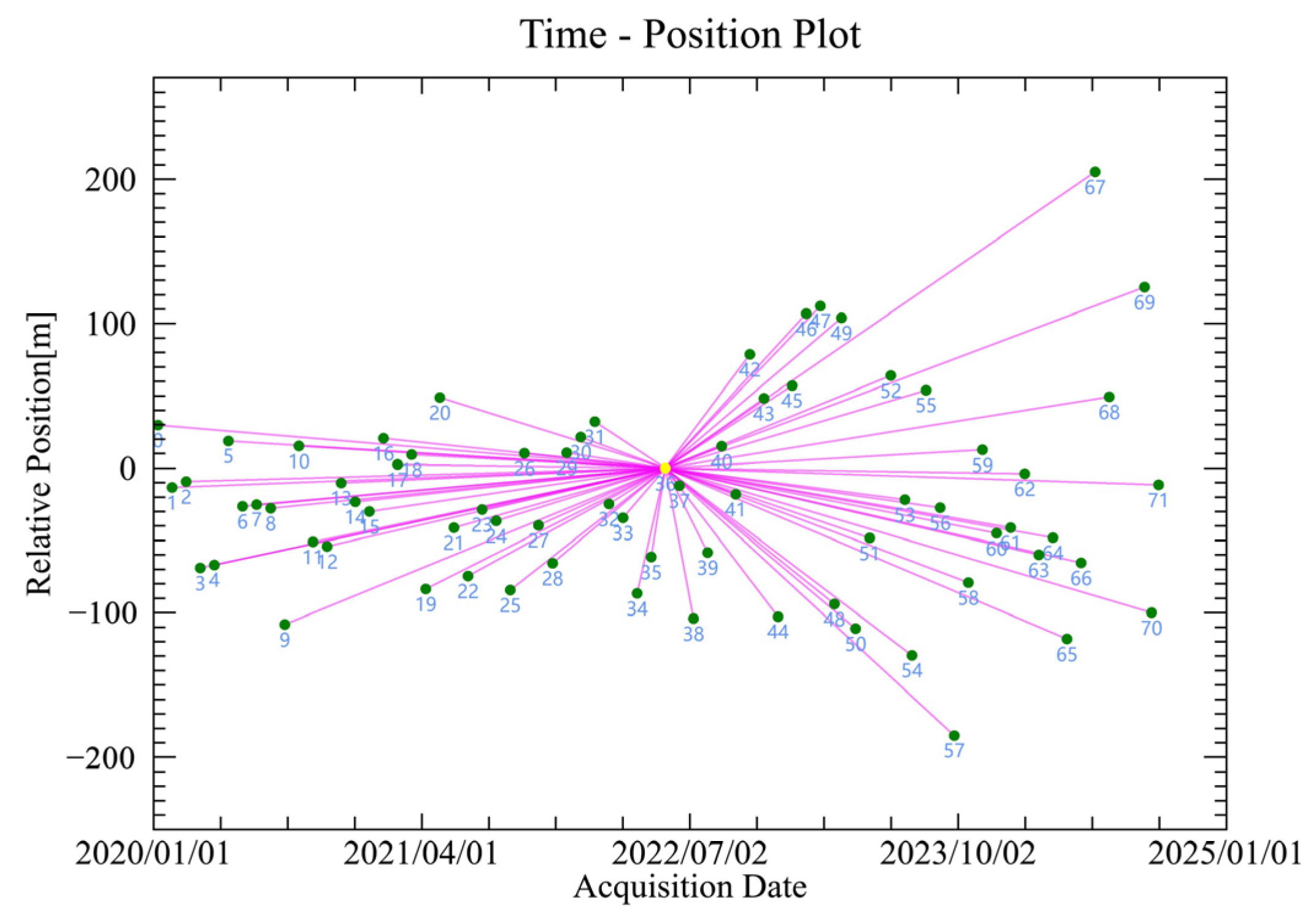
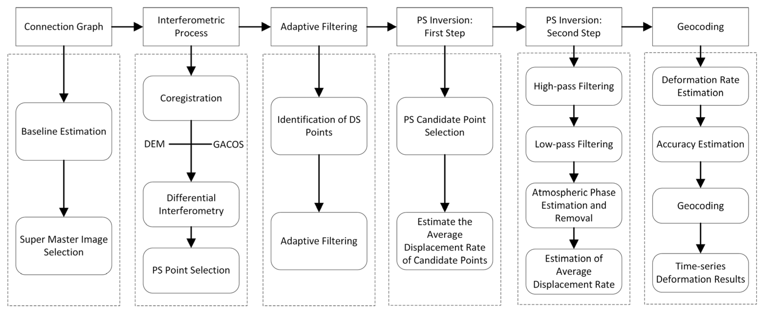
- PS-InSAR
- (2)
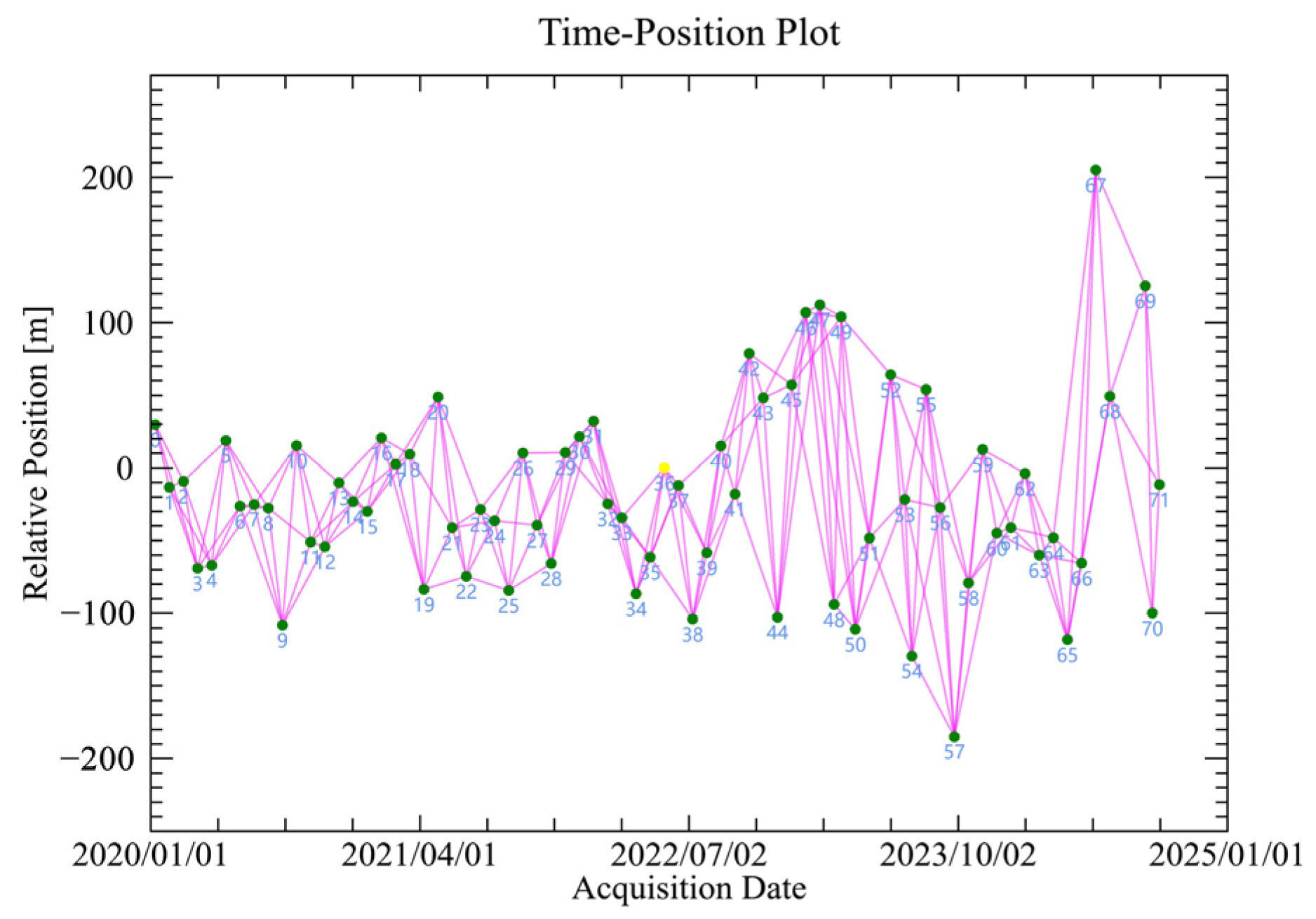
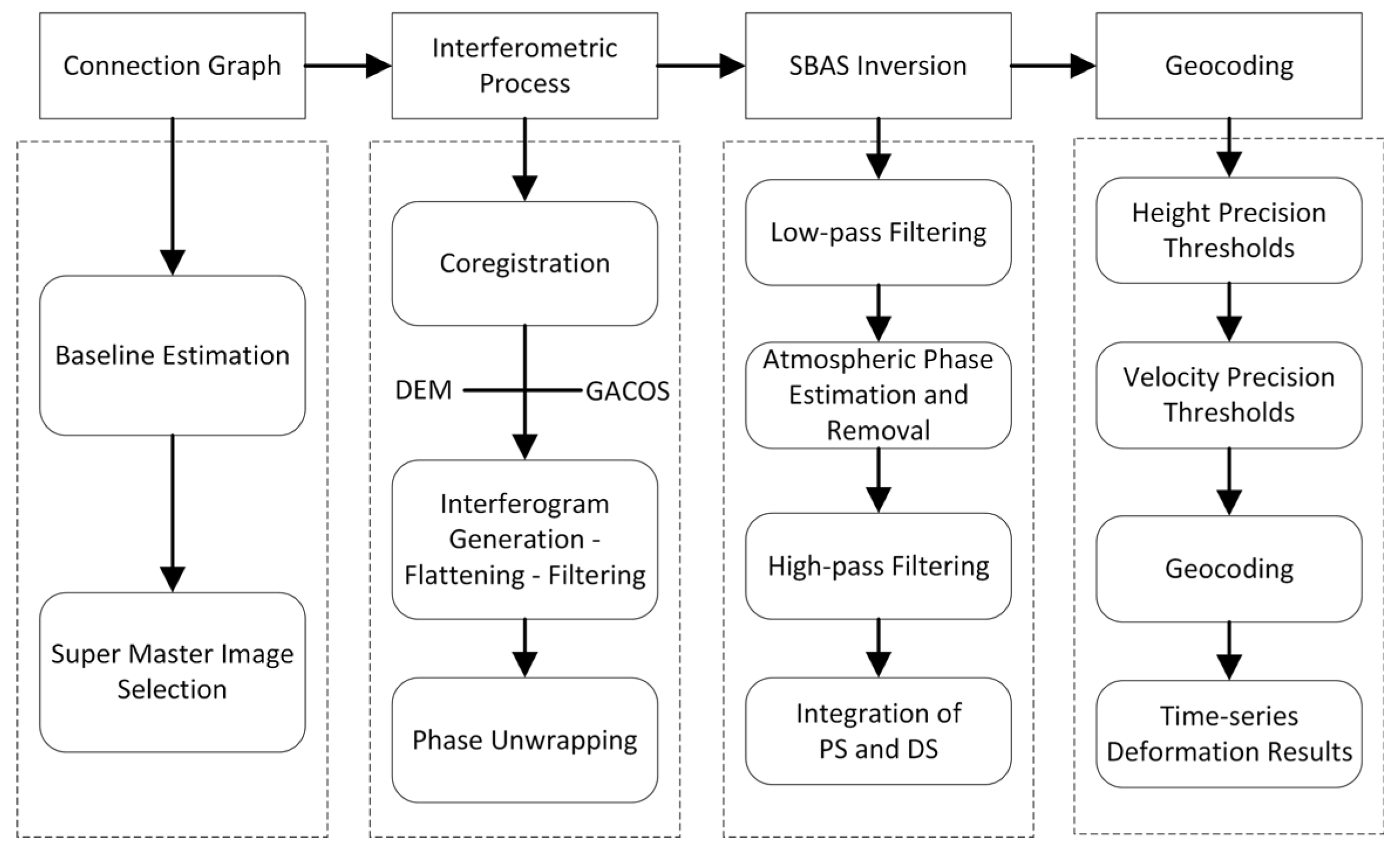
- SBAS-InSAR
2.3.2. The Gray System Theory
2.3.3. Surface Deformation Prediction Model
- (1)
- LSTM
- (2)
- Transformer
- (3)
- Efficient Additive Attention
- (4)
- LE-Transformer Model Architecture
- (1)
- Data preprocessing module: The data preprocessing module normalizes the input data to a range between 0 and 1, improving the training efficiency and accuracy of the model. This operation ensures that the data can be effectively handled in subsequent modules, laying the foundation for accurate feature learning by the model.
- (2)
- LSTM module: The LSTM module initializes hidden states and cell states before performing forward propagation through LSTM layers. It outputs features that contain rich temporal information about the input sequences, providing a robust representation for the subsequent attention mechanism.
- (3)
- EAA Module: The EAA module transforms the input embedding matrix into query and key matrices through specific matrix operations, followed by normalization. The query matrix is multiplied by a learnable vector to generate attention weights, producing a global attention query vector. This query vector is pooled into a single global query vector, and element-wise multiplication is applied to encode its interaction with the key matrix to form a global context. EAA replaces traditional matrix multiplications with linear operations, reducing computational complexity. By precisely focusing on key factors in multivariate data, this module provides weighted features to the Transformer module, enabling the model to capture critical information and enhance the accuracy of pit deformation prediction.
- (4)
- Transformer module: The Transformer module processes the weighted features provided by the EAA module. Using its multi-head self-attention mechanism, it captures global dependencies in the data. The module further employs a feedforward network for nonlinear transformations, while residual connections and layer normalization help mitigate gradient issues during the training of deep networks.
- (5)
- Output layer: The features processed by the Transformer module are passed to a fully connected layer. This layer adjusts weight based on the training data, mapping the input features to the final predicted values. The output layer generates accurate predictions for pit deformation.

- (5)
- Training and Evaluation
3. Results
3.1. InSAR Monitoring Results
3.2. Analysis of Influencing Factors
3.3. LE-Transformer Prediction Results
3.4. Comparison with Other Models
4. Discussion
5. Conclusions
- (1)
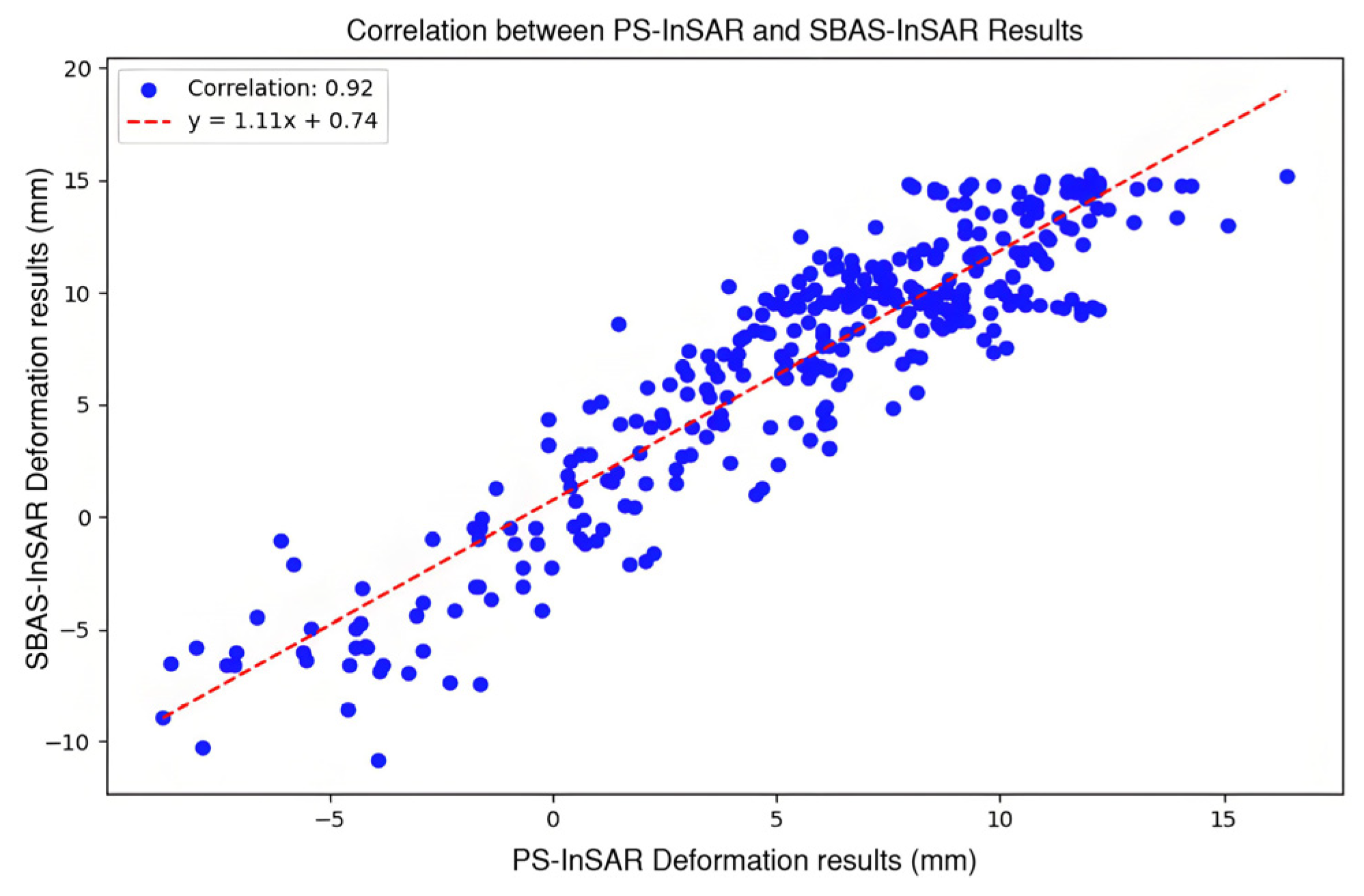
- Deformation data for the 220 kV Port Substation foundation pit in Guangzhou’s Nansha District were obtained using two InSAR techniques, PS-InSAR and SBAS-InSAR. The cumulative deformation ranged from −10 mm to +15 mm, with a high correlation coefficient of 0.92 between the results from both methods. This demonstrates the effectiveness of InSAR-based monitoring for large-scale urban infrastructure projects, offering superior coverage and precision compared to traditional methods.
- (2)
- Gray relational analysis identified key factors affecting deformation, including rainfall, subway construction, residential buildings, soil temperature, and hydrogeology. Rainfall was the most influential factor, with a correlation of 0.838. These findings underscore the importance of considering both environmental and infrastructural factors in foundation pit settlement, which is crucial for risk management in urban development projects.
- (3)
- The LE-Transformer model outperformed traditional prediction models, achieving a mean absolute percentage error (MAPE) of 2.5%. By incorporating both spatial and temporal data, the model demonstrated superior capability in predicting complex deformation trends. Its ability to handle multivariate data provides a more comprehensive understanding of the deformation mechanisms in foundation pit projects.
Author Contributions
Funding
Data Availability Statement
Conflicts of Interest
References
- Zhou, Y.; Su, W.; Ding, L.; Luo, H.; Love, P.E. Predicting safety risks in deep foundation pits in subway infrastructure projects: Support vector machine approach. J. Comput. Civ. Eng. 2017, 31, 04017052. [Google Scholar] [CrossRef]
- Xie, Z.; Tu, F. Reliability analysis of electronic total station and inclinometer in deformation monitoring of foundation pit. Geotech. Investig. Surv. 2009, 37, 81–84. [Google Scholar]
- Zhang, W.; Xiang, D.; Yu, Z.; Hua, X. Horizontal displacement monitoring and results analysis of pit surveyed by total station. Surv. Mapp. Geol. Miner Resour. 2009, 25, 4–6. [Google Scholar]
- Wu, J.; Peng, L.; Li, J.; Zhou, X.; Zhong, J.; Wang, C.; Sun, J. Rapid safety monitoring and analysis of foundation pit construction using unmanned aerial vehicle images. Autom. Constr. 2021, 128, 103706. [Google Scholar]
- Wang, Y.; Feng, G.; Li, Z.; Luo, S.; Wang, H.; Xiong, Z.; Zhu, J.; Hu, J. A Strategy for Variable-Scale InSAR Deformation Monitoring in a Wide Area: A Case Study in the Turpan–Hami Basin, China. Remote Sens. 2022, 14, 3832. [Google Scholar] [CrossRef]
- Zhang, G.; Xu, Z.; Chen, Z.; Wang, S.; Liu, Y.; Gong, X. Analyzing surface deformation throughout China’s territory using multi-temporal InSAR processing of Sentinel-1 radar data. Remote Sens. Environ. 2024, 305, 114105. [Google Scholar] [CrossRef]
- Zhang, J.; Ke, C.; Shen, X.; Lin, J.; Wang, R. Monitoring Land Subsidence along the Subways in Shanghai on the Basis of Time-Series InSAR. Remote Sens. 2023, 15, 908. [Google Scholar] [CrossRef]
- Sun, L.; Liu, S.; Zhang, L.; He, K.; Yan, X. Prediction of the displacement in a foundation pit based on neural network model fusion error and variational modal decomposition methods. Measurement 2025, 240, 115534. [Google Scholar] [CrossRef]
- Li, Q.; Yao, C.; Yao, X.; Zhou, Z.; Ren, K. Time Series Prediction of Reservoir Bank Slope Deformation Based on Informer and InSAR: A Case Study of Dawanzi Landslide in the Baihetan Reservoir Area, China. Remote Sens. 2024, 16, 2688. [Google Scholar] [CrossRef]
- Du, J.; Yin, K.; Lacasse, S. Displacement prediction in colluvial landslides, Three Gorges Reservoir, China. Landslides 2012, 10, 203–218. [Google Scholar] [CrossRef]
- Shi, J.; Wang, S.; Qu, P.; Shao, J. Time series prediction model using LSTM-Transformer neural network for mine water inflow. Sci. Rep. 2024, 14, 18284. [Google Scholar] [CrossRef] [PubMed]
- Li, W.; Law, K.L.E. Deep Learning Models for Time Series Forecasting: A Review. IEEE Access 2024, 12, 92306–92327. [Google Scholar] [CrossRef]
- Li, Y.; Zhu, Z.; Kong, D.; Han, H.; Zhao, Y. EA-LSTM: Evolutionary attention-based LSTM for time series prediction. Knowl.-Based Syst. 2019, 181, 104785. [Google Scholar] [CrossRef]
- Chen, Y.; He, Y.; Zhang, L.; Chen, B.; He, X.; Pu, H.; Cao, S.; Gao, L.; Yang, W. Surface deformation prediction based on TS-InSAR technology and long short-term memory networks. Natl. Remote Sens. Bull. 2022, 26, 1326–1341. [Google Scholar] [CrossRef]
- Bharti, M.K.; Wadhvani, R.; Gyanchandani, M.; Gupta, M. Transformer-Based Multivariate Time Series Forecasting. In Proceedings of the 2024 IEEE International Students’ Conference on Electrical, Electronics and Computer Science (SCEECS), Bhopal, India, 24–25 February 2024; pp. 1–6. [Google Scholar]
- Wang, J.; Li, C.; Li, L.; Huang, Z.; Wang, C.; Zhang, H.; Zhang, Z. InSAR time-series deformation forecasting surrounding Salt Lake using deep transformer models. Sci. Total Environ. 2023, 858, 159744. [Google Scholar] [CrossRef]
- Tong, G.; Ge, Z.; Peng, D. RSMformer: An efficient multiscale transformer-based framework for long sequence time-series forecasting. Appl. Intell. 2024, 54, 1275–1296. [Google Scholar] [CrossRef]
- Zhang, J.; Luo, Z.; Yang, Z. Research on Air Quality Prediction Based on LSTM-Transformer with Adaptive Temporal Attention Mechanism. In Proceedings of the 2023 2nd International Conference on Artificial Intelligence and Intelligent Information Processing (AIIIP), Hangzhou, China, 27–29 October 2023; pp. 320–323. [Google Scholar]
- Ferretti, A.; Prati, C.; Rocca, F. Permanent scatterers in SAR interferometry. IEEE Trans. Geosci. Remote Sens. 2001, 39, 8–20. [Google Scholar] [CrossRef]
- Ferretti, A.; Fumagalli, A.; Novali, F.; Prati, C.; Rocca, F.; Rucci, A. A New Algorithm for Processing Interferometric Data-Stacks: SqueeSAR. IEEE Trans. Geosci. Remote Sens. 2011, 49, 3460–3470. [Google Scholar] [CrossRef]
- Fornaro, G.; Verde, S.; Reale, D.; Pauciullo, A. CAESAR: An Approach Based on Covariance Matrix Decomposition to Improve Multibaseline–Multitemporal Interferometric SAR Processing. IEEE Trans. Geosci. Remote Sens. 2015, 53, 2050–2065. [Google Scholar] [CrossRef]
- Liu, Y.; Fan, H.; Wang, L.; Zhuang, H. Monitoring of surface deformation in a low coherence area using distributed scatterers InSAR: Case study in the Xiaolangdi Basin of the Yellow River, China. Bull. Eng. Geol. Environ. 2020, 80, 25–39. [Google Scholar] [CrossRef]
- Ye, K.; Wang, Z.; Wang, T.; Luo, Y.; Chen, Y.; Zhang, J.; Cai, J. Deformation Monitoring and Analysis of Baige Landslide (China) Based on the Fusion Monitoring of Multi-Orbit Time-Series InSAR Technology. Sensors 2024, 24, 6760. [Google Scholar] [CrossRef] [PubMed]
- Berardino, P.; Fornaro, G.; Lanari, R.; Sansosti, E. A new algorithm for surface deformation monitoring based on small baseline differential SAR interferograms. IEEE Trans. Geosci. Remote Sens. 2002, 40, 2375–2383. [Google Scholar] [CrossRef]
- Lanari, R.; Mora, O.; Manunta, M.; Mallorquí, J.J.; Berardino, P.; Sansosti, E. A small-baseline approach for investigating deformations on full-resolution differential SAR interferograms. IEEE Trans. Geosci. Remote Sens. 2004, 42, 1377–1386. [Google Scholar] [CrossRef]
- Parizzi, A.; Brcic, R.; De Zan, F. InSAR performance for large-scale deformation measurement. IEEE Trans. Geosci. Remote Sens. 2020, 59, 8510–8520. [Google Scholar]
- Chen, Y.; Yu, S.; Tao, Q.; Liu, G.; Wang, L.; Wang, F. Accuracy Verification and Correction of D-InSAR and SBAS-InSAR in Monitoring Mining Surface Subsidence. Remote Sens. 2021, 13, 4365. [Google Scholar] [CrossRef]
- Du, Q.; Li, G.; Zhou, Y.; Chai, M.; Chen, D.; Qi, S.; Wu, G.; Zhao, X.D. Deformation Monitoring in an Alpine Mining Area in the Tianshan Mountains Based on SBAS-InSAR Technology. Adv. Mater. Sci. Eng. 2021, 2021, 9988017. [Google Scholar] [CrossRef]
- Sun, Y.; Liu, S.; Li, L. Grey Correlation Analysis of Transportation Carbon Emissions under the Background of Carbon Peak and Carbon Neutrality. Energies 2022, 15, 3064. [Google Scholar] [CrossRef]
- Tsai, M.-S.; Hsu, F.-Y. Application of Grey Correlation Analysis in Evolutionary Programming for Distribution System Feeder Reconfiguration. IEEE Trans. Power Syst. 2010, 25, 1126–1133. [Google Scholar] [CrossRef]
- Sherstinsky, A. Fundamentals of Recurrent Neural Network (RNN) and Long Short-Term Memory (LSTM) network. Phys. D Nonlinear Phenom. 2020, 404, 132306. [Google Scholar] [CrossRef]
- Waqas, M.; Humphries, U.W. A critical review of RNN and LSTM variants in hydrological time series predictions. MethodsX 2024, 13, 102946. [Google Scholar] [CrossRef]
- Liu, J.; Xu, T.; Lu, C.; Yang, J.; Xie, Y. Variational mode decomposition coupled LSTM with encoder-decoder framework: An efficient method for daily streamflow forecasting. Earth Sci. Inform. 2024, 18, 38. [Google Scholar] [CrossRef]
- Singh, U.; Saurabh, K.; Trehan, N.; Vyas, R.; Vyas, O.P. GA-LSTM: Performance Optimization of LSTM driven Time Series Forecasting. Comput. Econ. 2024, 1–36. [Google Scholar] [CrossRef]
- Tamilselvi, C.; Paul, R.K.; Yeasin, M.; Paul, A.K. Novel wavelet-LSTM approach for time series prediction. Neural Comput. Appl. 2024, 1–10. [Google Scholar] [CrossRef]
- Meng, X.; Yang, Y.; Wang, L.; Wang, T.; Li, R.; Zhang, C. Class-Guided Swin Transformer for Semantic Segmentation of Remote Sensing Imagery. IEEE Geosci. Remote Sens. Lett. 2022, 19, 6517505. [Google Scholar] [CrossRef]
- Qiu, Y.; Liu, Y.; Zhang, L.; Lu, H.; Xu, J. Boosting Salient Object Detection with Transformer-Based Asymmetric Bilateral U-Net. IEEE Trans. Circuits Syst. Video Technol. 2024, 34, 2332–2345. [Google Scholar] [CrossRef]
- Wang, S.; Wang, H.; She, S.; Zhang, Y.; Qiu, Q.; Xiao, Z. Swin-T-NFC CRFs: An encoder–decoder neural model for high-precision UAV positioning via point cloud super resolution and image semantic segmentation. Comput. Commun. 2023, 197, 52–60. [Google Scholar] [CrossRef]
- Xiao, T.; Liu, Y.; Huang, Y.; Li, M.; Yang, G. Enhancing Multiscale Representations with Transformer for Remote Sensing Image Semantic Segmentation. IEEE Trans. Geosci. Remote Sens. 2023, 61, 5605116. [Google Scholar] [CrossRef]
- Xiao, X.; Guo, W.; Chen, R.; Hui, Y.; Wang, J.; Zhao, H. A Swin Transformer-Based Encoding Booster Integrated in U-Shaped Network for Building Extraction. Remote Sens. 2022, 14, 2611. [Google Scholar] [CrossRef]
- Ye, X.; Fang, S.; Sun, F.; Zhang, C.; Xiang, S. Meta Graph Transformer: A Novel Framework for Spatial–Temporal Traffic Prediction. Neurocomputing 2022, 491, 544–563. [Google Scholar] [CrossRef]
- Zheng, Z.; Zhong, Y.; Tian, S.; Ma, A.; Zhang, L. ChangeMask: Deep multi-task encoder-transformer-decoder architecture for semantic change detection. ISPRS J. Photogramm. Remote Sens. 2022, 183, 228–239. [Google Scholar] [CrossRef]
- Fan, J.; Gao, B.; Ge, Q.; Ran, Y.; Zhang, J.; Chu, H. SegTransConv: Transformer and CNN Hybrid Method for Real-Time Semantic Segmentation of Autonomous Vehicles. IEEE Trans. Intell. Transp. Syst. 2024, 25, 1586–1601. [Google Scholar] [CrossRef]
- Ahmed, S.; Nielsen, I.E.; Tripathi, A.; Siddiqui, S.; Ramachandran, R.P.; Rasool, G. Transformers in Time-Series Analysis: A Tutorial. Circuits Syst. Signal Process. 2023, 42, 7433–7466. [Google Scholar] [CrossRef]
- Kim, G.h.; Kim, E. Stacked encoder–decoder transformer with boundary smoothing for action segmentation. Electron. Lett. 2022, 58, 972–974. [Google Scholar] [CrossRef]
- Shaker, A.; Maaz, M.; Rasheed, H.; Khan, S.; Yang, M.-H.; Khan, F.S. Swiftformer: Efficient additive attention for transformer-based real-time mobile vision applications. In Proceedings of the IEEE/CVF International Conference on Computer Vision, Paris, France, 1–6 October 2023; pp. 17425–17436. [Google Scholar]
- Ma, Y.Y.; Chen, Y.B.; Zuo, X.Q.; Ma, W.F.; Wu, W.H. Analysis of land subsidence in Kunming based on SentineFlA data and SBAS technolog. Sci. Surv. Mapp. 2019, 44, 59–66+95. [Google Scholar] [CrossRef]
- Li, H.X.; Zhao, X.H.; Chi, H.Y.; Zhang, J.J. Prediction and Analysis of Land Subsidence Based on Improved BP Neural Network Model. J. Tianjin Univ. 2009, 42, 60–64. [Google Scholar]
- Mueller, T.G.; Pusuluri, N.B.; Mathias, K.K.; Cornelius, P.L.; Barnhisel, R.I.; Shearer, S.A. Map Quality for Ordinary Kriging and Inverse Distance Weighted Interpolation. Soil Sci. Soc. Am. J. 2004, 68, 2042–2047. [Google Scholar] [CrossRef]
- Ma, F.; Sui, L.; Lian, W. Prediction of Mine Subsidence Based on InSAR Technology and the LSTM Algorithm: A Case Study of the Shigouyi Coalfield, Ningxia (China). Remote Sens. 2023, 15, 2755. [Google Scholar] [CrossRef]


| Controlling Factor | Subway Construction | Housing Construction | Rainfall | Soil Temperature | Hydrogeology |
|---|---|---|---|---|---|
| Relatedness | 0.731 | 0.725 | 0.838 | 0.796 | 0.824 |
| Self-Attention Type | MSE | MAE | Complexity |
|---|---|---|---|
| EAA | 0.085 | 0.122 | O(n × d) |
| Multi-Head Attention | 0.156 | 0.232 | O(n2 × d) |
| Scaled Dot-Product Attention | 0.183 | 0.283 | O(n2 × d) |
| Models | MSE | MAPE | RMSE | R2 |
|---|---|---|---|---|
| GRU | 0.238 | 0.048 | 0.412 | 0.835 |
| LSTM | 0.215 | 0.042 | 0.384 | 0.857 |
| Transformer | 0.195 | 0.039 | 0.369 | 0.886 |
| LE-Transformer | 0.125 | 0.025 | 0.292 | 0.934 |
Disclaimer/Publisher’s Note: The statements, opinions and data contained in all publications are solely those of the individual author(s) and contributor(s) and not of MDPI and/or the editor(s). MDPI and/or the editor(s) disclaim responsibility for any injury to people or property resulting from any ideas, methods, instructions or products referred to in the content. |
© 2025 by the authors. Licensee MDPI, Basel, Switzerland. This article is an open access article distributed under the terms and conditions of the Creative Commons Attribution (CC BY) license (https://creativecommons.org/licenses/by/4.0/).
Share and Cite
Hu, B.; Li, W.; Lu, W.; Zhao, F.; Li, Y.; Li, R. Integrating InSAR Data and LE-Transformer for Foundation Pit Deformation Prediction. Remote Sens. 2025, 17, 1106. https://doi.org/10.3390/rs17061106
Hu B, Li W, Lu W, Zhao F, Li Y, Li R. Integrating InSAR Data and LE-Transformer for Foundation Pit Deformation Prediction. Remote Sensing. 2025; 17(6):1106. https://doi.org/10.3390/rs17061106
Chicago/Turabian StyleHu, Bo, Wen Li, Weifeng Lu, Feilong Zhao, Yuebin Li, and Rijun Li. 2025. "Integrating InSAR Data and LE-Transformer for Foundation Pit Deformation Prediction" Remote Sensing 17, no. 6: 1106. https://doi.org/10.3390/rs17061106
APA StyleHu, B., Li, W., Lu, W., Zhao, F., Li, Y., & Li, R. (2025). Integrating InSAR Data and LE-Transformer for Foundation Pit Deformation Prediction. Remote Sensing, 17(6), 1106. https://doi.org/10.3390/rs17061106