Dual-Branch Diffusion Detection Model for Photovoltaic Array and Hotspot Defect Detection in Infrared Images

Abstract

Failures in solar photovoltaic (PV) modules generate heat, leading to various hotspots observable in infrared images. Automated hotspot detection technology enables rapid fault identification in PV systems, while PV array detection, leveraging geometric cues from infrared images, facilitates the precise localization of defects. This study tackles the complexities of detecting PV array regions and diverse hotspot defects in infrared imaging, particularly under the conditions of complex backgrounds, varied rotation angles, and the small scale of defects. The proposed model encodes infrared images to extract semantic features, which are then processed through an PV array detection branch and a hotspot detection branch. The array branch employs a diffusion-based anchor-free mechanism with rotated bounding box regression, enabling the robust detection of arrays with diverse rotational angles and irregular layouts. The defect branch incorporates a novel inside-awareness loss function designed to enhance the detection of small-scale objects. By explicitly modeling the dependency distribution between arrays and defects, this loss function effectively reduces false positives in hotspot detection. Experimental validation on a comprehensive PV dataset demonstrates the superiority of the proposed method, achieving a mean average precision (mAP) of 71.64% for hotspot detection and 97.73% for PV array detection.

1. Introduction

With the rising global demand for clean energy, solar power has gained significant attention as a reliable, green, and sustainable energy source. Photovoltaic (PV) cells, the core components of PV power generation systems, are interconnected in series and parallel to form PV modules, which are further grouped into PV panels [1]. PV panel defects, indicated by temperature anomalies, arise from factors such as module shielding, dirt accumulation, panel rupture, diode failure, and module fragmentation. In severe cases, these defects can lead to fires, posing significant safety risks to solar power plants (see

Table 1. The annotation information of the dataset. # Instances means number of instances.

Category	Description	#Instances	Size	Rotation *
Line	Hotspot caused by PV module shielding, bubble, delamination, dirt, and gate line fracture.	2283	Small target within $40\times 5$ or $5\times 40$	-
Flocculant	Hotspot caused by PV module occlusion, dirt, and rupture.	3310	Small target within $25\times 25$	-
Strip	Hotspot caused by PV module occlusion, dirt, diode failure, and bracket deformation.	3377	Small target within $40\times 20$ or $25\times 40$	-
Facet	Hotspot caused by PV module fragmentation, module failure, and module disconnection.	168	Small target within $40\times 30$ or $30\times 40$	-
Array	A complete power-generating unit, consisting of any number of PV modules and panels.	32,960	Rotated rectangles with various sizes	$[-{90}^{\circ },{90}^{\circ })$

* The rotation angle $\alpha \in [{90}^{\circ },{90}^{\circ })$ is determined by rotating the rectangle counterclockwise, aligning the longer side w with the x-axis for the first time.

) [2,3]. Early detection is essential to maintaining PV system efficiency and longevity. Overheating defects appear as various hotspot patterns in thermal imaging, making handheld thermal imaging devices a common tool for PV module monitoring. However, the widespread distribution of PV power plants across diverse environments, such as ground installations, water surfaces, and rooftops, makes manual inspection both time-consuming and inefficient [4]. Infrared thermal imaging, which converts thermal radiation into temperature-based images, offers a rapid and effective method for identifying surface temperature anomalies on PV panels. Figure 1 presents representative infrared images of PV arrays, showcasing various types of hotspot defects. However, several factors complicate the detection process in practical scenarios. These include unknown image resolution, environmental background interference, and the arrangement of PV panels. Additionally, accurately detecting hotspots is further challenged by background noise, the small size of the targets, and environmental variability. This emphasizes the need for more robust and precise detection algorithms [5,6].

In practice, the PV array and hotspot detection leverages UAV-mounted infrared imaging to automatically locate PV panel failures. The whole process can be simplified into four procedure, as illustrated in Figure 2.

(1)

A UAV equipped with an infrared imager patrols the photovoltaic power station, capturing high-resolution infrared images of photovoltaic modules.

(2)

The images are uploaded to a local or remote server, where the PV array and hotspot detection model analyzes them.

(3)

The model processes the infrared images to detect and pinpoint the positions of photovoltaic strings and fault hotspots. By integrating GPS information from the images, precise fault locations are determined swiftly.

(4)

Armed with this detection information, maintenance personnel can promptly access and address identified faults, optimizing maintenance efficiency and minimizing downtime.

Figure 2. PV array and hotspot detection applied in practical power station maintenance.

Figure 2. PV array and hotspot detection applied in practical power station maintenance.

1.1. Related Works

Benefiting from the development of various machine learning theories, research on PV panel hotspot detection using infrared images has explored both shallow and deep learning methods. Dotenko et al. [7] utilized Grubbs’ hypothesis test and Dixon’s hypothesis test to identify the components containing hotspots, leveraging features such as median component temperature and histogram projections. Similarly, Jiang Lin et al. [8] addressed the challenge of random noise in infrared images by introducing a B-spline least squares method based on grayscale histograms, combined with the Canny operator for hotspot detection. The shallow learning methods rely on handcrafted features and thus are limited by their susceptibility to noise and environmental variability. In contrast, deep learning-based detectors, including Faster R-CNN [9], SSD [10], and YOLO [11], demonstrate significant potential.

The environment of PV power stations is inherently complex. Due to the limited spatial resolution of infrared images and the challenges of long-distance imaging, PV hotspots often appear as small targets. Furthermore, as network depth increases in deep learning models, feature information tends to degrade, reducing feature discrimination under the interference from complex backgrounds [12]. As a result, directly applying models like YOLO and Faster R-CNN for detecting PV hotspots in infrared images frequently leads to missed detections and false positives. To address these challenges, Zhao et al. [13] developed two end-to-end modules, namely the Neighborhood Correlation Feature Module (NCFM) for multi-scale feature learning and the Scale-aware Attention Mechanism (SAM) for enhanced feature utilization. Hao et al. [14] introduced a hotspot detection algorithm combining a feature pyramid with a high-resolution network. While these methods improve feature extraction, some researchers believe the non-photovoltaic regions such as the normal PV arrays have an impact on detection accuracy. By accounting for the array regions, Qian et al. [15] devised a stepwise fault diagnosis strategy, combining segmentation and detection to focus the algorithm on hotspot areas. Likewise, Yu et al. [16] presented a Deeplab-YOLO detection method that integrated an optimized Deeplabv3+ model with YOLO v5. The primary limitation of the two-stage approach lies in its reliance on the quality of array segmentation results from the first stage, which significantly impacts the overall detection accuracy.

Thermal imaging is widely used for defect detection beyond PV inspections. For instance, Zahradník et al. [17] employed a U-Net model for flat roof classification and thermal-based leak detection. In industrial inspections, Li et al. [18] developed a UAV-based thermal imaging system with YOLOX for bird nest detection, while Mei et al. [19] enhanced power equipment failure detection using a modified Faster R-CNN with DenseNet. Traditional methods remain relevant as well; Liao et al. [20] applied segmentation and filtering techniques to assess composite material defects in aircrafts. Given these diverse approaches, balancing deep learning and traditional methods in infrared defect detection is crucial. Deep learning excels in feature extraction and complex environments but may be computationally demanding for small PV systems. Traditional image processing, while resource-efficient, offers less flexibility in varying conditions.

Recent studies [21,22,23,24,25] have shown promising results by adapting diffusion processes for object detection. This success can be attributed to two key factors. First, the iterative denoising process provides fine-grained control over generation steps, which aligns seamlessly with the iterative nature of object detection—progressively refining bounding boxes and classifications. Second, diffusion models are highly effective at modeling complex data distributions without the need for adversarial training, which is often unstable. This strength makes them particularly well-suited for detecting objects in diverse and intricate scenes. DiffusionDet [22] frames the object detection task as a denoising diffusion process. During training, the model begins with random noise bounding boxes ${\mathit{b}}_t\in {\mathbb{R}}^{N\times 4}\sim \mathcal{N}(\mathsf{\mu },\Sigma )$ and gradually learns to transform these noisy boxes into accurate object boxes through a trained neural network $D_{\theta }\left({\mathit{b}}_0\right|{\mathit{b}}_t)={\prod }_{k=0}^t{p}_{\theta }\left({\mathit{b}}_{t-k}\right|{\mathit{b}}_{t-k+1})$. In the inference phase, DiffusionDet starts with randomly initialized bounding boxes sampled from $p\left({\mathit{b}}_t\right)$ and applies the learned $D_{\theta }\left({\mathit{b}}_0\right|{\mathit{b}}_t)$ to iteratively refine the predicted boxes. Likewise, DiffAD [23] and Diff3D [25] employ specialized networks to model the denoising diffusion process. DiffAD predicts the ground truth from a randomly sampled action distribution, while Diff3D focuses on predicting the 3D target box.

While existing studies have achieved success in detecting general objects, actions, and 3D objects, research on detecting small or oriented objects remains blank. To summarize, developing highly efficient and precise hotspot detection algorithms faces the following challenges. First, the diverse background characteristics of PV power stations, combined with low-resolution images, small target size, and blurred boundaries, present significant challenges for deep learning models to generalize effectively [26]. Second, while considering the positional relationship between PV arrays and hotspot defects can improve detection rates, the two-stage strategy by segmenting arrays first and detecting hotspots afterward introduces a detection bottleneck [27]. Effectively modeling the interrelationship between arrays and hotspots is crucial for enhancing detection performance. Third, PV arrays are large-scale targets with high sample volumes, while hotspots are small-scale targets with low sample volumes. Addressing the challenges of class imbalance and target size disparity is another key for designing hotspot detection models.

1.2. Motivations and Novelties

To address the aforementioned three challenges, we propose a dual-branch PV array and hotspot defect detection model. The motivations and contributions of the proposed model are emphasized in this section.

1.2.1. Motivations

To begin with, let us demonstrate the necessity of localizing PV arrays. On the one hand, in practical operations and maintenance, localizing PV arrays allows maintenance personnel to quickly pinpoint the geographic location of hotspot defects [28,29]. On the other hand, PV hotspot defects are always located on arrays, making the modeling of this positional dependency a potential way to improve model robustness. However, the existing studies often treat array detection and hotspot detection as independent tasks, limiting their ability to exploit the dependency. Consequently, the first motivation of this study is to process array and hotspot detection collaboratively. To achieve this, we propose a dual-branch detection model consisting of two detection branches—one for PV arrays and the other for hotspot defects. Both branches share a common backbone network to leverage shared low-level semantic features from the image. Each branch, however, is equipped with an independent detection head tailored to its specific task. The array detection head performs binary classification and rotated bounding box regression tasks, and the defect detection head handles multi-class classification and small bounding box regression tasks. The dual-branch architecture allows the model to resolve the class imbalance and scale disparity issues by designing attribute-specific modules.

The second motivation arises from the need to design specialized detection heads for each branch, with one for detecting large, rotated array targets and another for detecting small hotspot targets. The existing methods based on Faster R-CNN and YOLO series struggle to handle multiscale and rotated targets due to their fixed-scale anchor proposals. Inspired by DiffusionDet [22] and DiffAD [23], we adopt diffusion models to perform rotated array detection and hotspot detection. The feasibility and advantage can be perceived from three aspects. First, the diffusion model formulates object detection as a denoising diffusion process by transforming noisy boxes into object boxes, which requires neither heuristic object priors nor learnable queries. The anchor-free property makes it promising for overcoming the low angle sensitivity issue in array detection, as well as the target-scale adaptation issue in defect detection. Second, the iterative denoising nature of the diffusion process is well-suited for bounding box refinement. By progressively refining the bounding box across multiple diffusion steps, we can more accurately localize hotspot defects in infrared images, where noise and ambiguous features complicate detection. Third, diffusion models enhance the detection of small objects by utilizing their denoising capability through multiple steps. This iterative process reduces false positives and improves detection precision, especially for small defects.

The final motivation is to explicitly represent the dependency relationship between PV arrays and hotspot defects. Beyond sharing low-level image information at the feature level, we incorporate the array–defect dependencies directly into the model’s loss function. The dependency can be abstracted by the following:

$$P(X\in {\mathsf{\Omega }}_{\mathrm{defect}}|X\in {\mathsf{\Omega }}_{\mathrm{array}})\ne 0,P(X\in {\mathsf{\Omega }}_{\mathrm{defect}}|X\notin {\mathsf{\Omega }}_{\mathrm{array}})=0,$$

(1)

where ${\mathsf{\Omega }}_{\mathrm{defect}},{\mathsf{\Omega }}_{\mathrm{array}}$ represent the defect and array regions. As observed from (1), our intention is to model the conditional distribution with a specifically defined inside-awareness loss. This loss function is designed to penalize cases where hotspot defects are detected outside array regions, while simultaneously encouraging the model to generate small-scale and consistent-scale bounding boxes for hotspots.

1.2.2. Novelties

Based on the aforementioned motivations, we propose a dual-branch photovoltaic array and hotspot collaborative detection model. The key contributions of this study are summarized as follows:

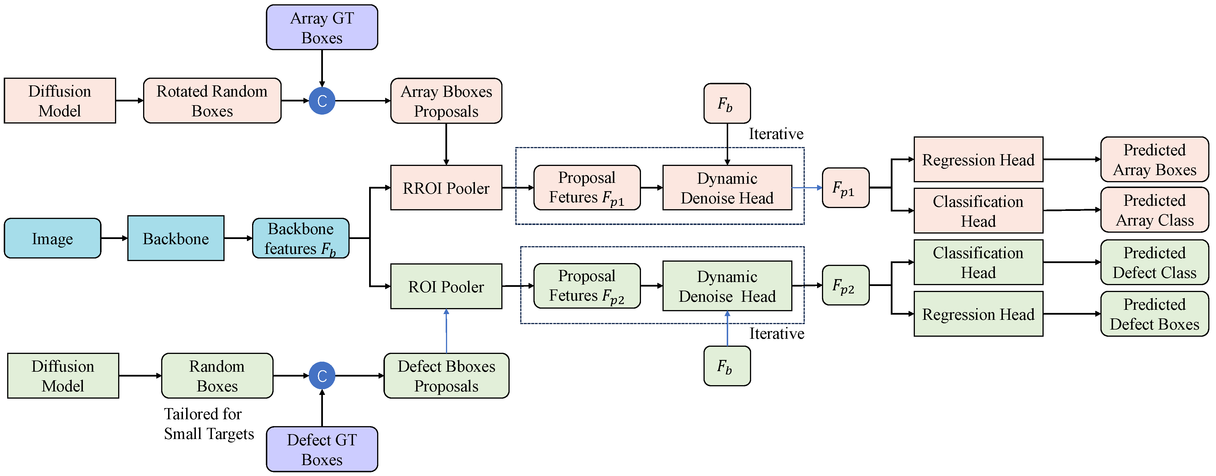
• A dual-branch detection network architecture is proposed. The proposed network includes two branches—one for PV arrays and the other for hotspot defects. The branches share low-level image features to model their correlations, while possessing independent detection heads to learn high-level semantic features. This separable architecture enhances the flexibility of the network, alleviating the class imbalance and scale disparity issues between arrays and hotspots.
• A diffusion-based rotated bounding box detection branch is introduced for photovoltaic arrays, alongside a small-object detection branch for hotspot defects. The anchor-free nature of the diffusion-based approach improves sensitivity to rotation angles and adaptability to varying target scales.
• The inside-awareness loss function is developed for the dual-branch model to explicitly model the dependency distribution between arrays and defects. This loss function penalizes deviation in their internal and external relationships, guiding the model to learn from the bounding boxes for the hotspot defects located within arrays. The inside-awareness loss comprises two components—Inside IoU and Union-over-Convex-Hull loss. These terms guide the model to generate bounding boxes with compact scales and consistent scale ratios. The experimental results demonstrate that this loss significantly enhances the robustness of the detection model.

2. Preliminaries

The denoising diffusion probabilistic model [30] and its variants [31,32,33,34] are a series of generative models consisting of the forward diffusion process and the reversing denoising process. The diffusion process projects natural distributions into a prior distribution, typically a Gaussian, by iteratively adding noise. Formally, given a data sample $x_0$, considering its state at timestamp t, denoted as $x_t$, is generated as follows:

$$q\left(x_t\right|x_{t-1})=\mathcal{N}(x_t;\sqrt{1-{\beta }_t}{x}_{t-1},{\beta }_{t}I),$$

(2)

where ${\beta }_t$ is an empirical parameter controlling noise variance at timestep t. The denoising process learns to reverse the forward process, i.e., starting from pure noise and gradually removing noise to restore the original data distributions. Mathematically, the reverse process aims to learn the conditional probability distribution $p_{\theta }\left(x_{t-1}\right|x_t)$ as follows:

$$p_{\theta }\left(x_{t-1}\right|x_t)=\mathcal{N}(x_{t-1};{\mu }_{\theta }(x_t,t),{\Sigma }_{\theta }(x_t,t)),$$

(3)

where ${\mu }_{\theta }$ and ${\Sigma }_{\theta }$ represent the mean and covariance, respectively, and are parameterized by $\theta$, often implemented using neural networks. By modeling and training these two processes, the diffusion models are capable of generating high-quality data samples from noise.

In this work, we propose a dual-branch diffusion pipeline to address small and oriented object detection tasks simultaneously. The bounding boxes of the defect samples ${\mathit{b}}_0^{\mathrm{D}}\in {\mathbb{R}}^{N\times 4}$ and the array samples ${\mathit{b}}_0^{\mathrm{A}}\in {\mathbb{R}}^{N\times 5}$ are predicted using a shared image encoder $f_{{\Theta }_1}\left(\mathit{I}\right)$ and their respective denoising decoder $g_{{\Theta }_2^{\mathrm{D}}}\left({\mathit{b}}_0^{\mathrm{D}}\right|{\mathit{b}}_t^{\mathrm{D}},{\Theta }_1,\mathit{I})$ and $g_{{\Theta }_2^{\mathrm{A}}}\left({\mathit{b}}_0^{\mathrm{A}}\right|{\mathit{b}}_t^{\mathrm{A}},{\Theta }_1,\mathit{I})$, where the random ${\mathit{b}}_t^{\mathrm{D}}$ and ${\mathit{b}}_t^{\mathrm{A}}$ are sampled from their respective prior distributions.

3. Dual-Branch Photovoltaic Diagnose Network

This section outlines the proposed dual-branch photovoltaic diagnostic network. The framework is illustrated in Figure 3. Section 3.1 presents the overall structure of the dual-branch architecture. Section 3.2 and Section 3.3 detail the array branch and defect branch, respectively.

3.1. Dual-Branch Architecture

Image Encoder: In the context of object detection, the denoising process in the diffusion architecture corresponds to the iterative refinement of bounding boxes. As described in DiffusionDet, we employ bounding box alignment on the feature maps extracted by the image encoder to perform this refinement, thereby avoiding the high computational cost of directly iterating $g_{{\theta }_2}$ on the image. Both the array and defect branches share the same image encoder to emphasize their common characteristics. However, photovoltaic defects, being small targets, are particularly vulnerable to the loss of low-level texture information caused by down-sampling operations in multiple convolutional layers. To mitigate this, we incorporate a feature pyramid structure (FPN) into the encoder backbone to preserve low-level features. In the subsequent network, the shallow features p2 and p3 from FPN are utilized as inputs to the defect branch, while the semantic features p4, p5, and p6 are fed into the array branch.

Denoising Decoder: The denoising decoder’s role is to capture the fine-grained, branch-specific features unique to each detection task. The decoder for the array branch takes the semantic features from FPN and the proposal features aligned using the Rotated Region of Interest (RROI) Pooler for randomly rotated bounding boxes as input. It employs a multi-layer dynamic denoising head to iteratively refine these representations. Similarly, the decoder for the defect branch uses the shallow features from the FPN and the proposal features aligned by the ROI Pooler for randomly small bounding boxes as input. This decoder also employs multi-layer denoising heads, but its weights are not shared with the array branch. To further integrate texture features into the decoders, particularly for the defect branch, each denoising head incorporates the corresponding FPN features as part of its input.

3.2. The Array Branch

The array branch primarily consists of randomly rotated bounding boxes generated by the diffusion process, an RROI module, a denoising decoder, a rotation box regression head, and a binary classification head. Unlike the horizontal bounding boxes used in [22], each rotated bounding box is represented as a five-dimensional vector $\mathit{b}={[c_x,c_y,w,h,\alpha ]}^{\mathrm{T}}$, including an additional rotation parameter $\alpha$. The rotation angle $\alpha \in [0°,360°)$, as illustrated in Figure 4, is normalized to $[0,2\pi )$ to facilitate Gaussian sampling. The random rotated bounding boxes are passed to the RROI module, which aligns the encoder features with the corresponding regions. The aligned RROI feature are then passed to denoising decoder and the functional heads.

Following the offset regression for object detection, we formulate the regression target of the rotated bounding box as follows:

$$\begin{array}{cc}\hfill \Delta c_x& ={\displaystyle \frac{1}{w}}\left(\left(c_x-{\widehat{c}}_x\right)cos\alpha +\left(c_y-{\widehat{c}}_y\right)sin\alpha \right),\hfill \\ \hfill \Delta c_y& ={\displaystyle \frac{1}{h}}\left(\left(c_y-{\widehat{c}}_y\right)cos\alpha -\left(c_x-{\widehat{c}}_x\right)sin\alpha \right),\hfill \\ \hfill \Delta w& =log{\displaystyle \frac{w}{\widehat{w}}},\Delta h=log{\displaystyle \frac{h}{\widehat{h}}},\hfill \\ \hfill \Delta \alpha & ={\displaystyle \frac{1}{2\pi }}\left(\left(\alpha -\widehat{\alpha }\right)mod2\pi \right),\hfill \end{array}$$

(4)

where $c_x$ and $c_y$ represent the ground truth offsets for the bounding box center, and w and h denote the width and height offsets. $\Delta \mathit{b}=[\Delta c_x,\Delta c_y,\Delta w,\Delta h,\Delta \alpha ]$ represents the target offset vector. These regression targets are normalized to account for variations in scale and ensure stable training. The rotation box regression head and the binary classification head take the output features of the denoising decoder as their inputs. During the training phase of the array branch, the loss function is a combination of the following three components: Smooth-L1 loss [9] for regression, generalized Intersection-over-Union (gIoU) loss [35] for bounding box alignment, and Binary Cross-Entropy loss (BCELoss) for classification. The loss function of the array branch is computed by the following equation:

$$L_{\mathrm{array}}={\lambda }_1^{\mathrm{A}}{L}_{\mathrm{smooth}-\mathrm{L}1}+{\lambda }_2^{\mathrm{A}}{L}_{\mathrm{gIoU}}+{\lambda }_3^{\mathrm{A}}{L}_{\mathrm{BCE}},$$

(5)

where ${\lambda }_1^{\mathrm{A}},{\lambda }_2^{\mathrm{A}},{\lambda }_3^{\mathrm{A}}$ are empirical parameters.

3.3. The Defect Branch

Similar to the array branch, the defect branch consists of the diffusion process, an ROI module, a unique denoising decoder, a regression head, and a multi-class classification head. As mentioned earlier, PV defects are typically small targets. To better simulate the randomness of defects during the generation of random boxes, the standard deviation of the Gaussian distribution for the width and height parameters is reduced, ensuring that most generated random boxes correspond to small targets. The primary distinction between the array branch and the defect branch lies in the loss function. In addition to the smooth-L1 loss, gIoU loss, and multi-class cross-entropy loss, the defect branch introduces an inside-awareness loss. An important observation is that PV defects are always located on PV arrays, whereas PV arrays do not necessarily contain defects. This dependency relationship constrains the conditions for defect detection, thereby improving the robustness of the detection model. The inside-awareness loss in the defect branch is specifically designed to capture this dependency.

Given a bounding box proposal ${\widehat{\mathfrak{B}}}^{\mathrm{D}}$ and a matching defect-arra-y ground truth pair $({\widehat{\mathfrak{B}}}^{\mathrm{D}},{\widehat{\mathfrak{B}}}^{\mathrm{D}})$, the inside-awareness loss is formulated by the following:

$$\begin{array}{cc}\hfill & \mathrm{IoU}={\displaystyle \frac{{\widehat{\mathfrak{B}}}^{\mathrm{D}}\cap {\mathfrak{B}}^{\mathrm{D}}}{{\mathfrak{B}}^{\mathrm{D}}\cup {\mathfrak{B}}^{\mathrm{D}}}},\hfill \\ \hfill & \mathrm{IIoU}={\displaystyle \frac{{\widehat{\mathfrak{B}}}^{\mathrm{D}}\cap {\mathfrak{B}}^{\mathrm{A}}}{{\widehat{\mathfrak{B}}}^{\mathrm{D}}}},\hfill \\ \hfill & \mathrm{UoC}={\displaystyle \frac{{\widehat{\mathfrak{B}}}^{\mathrm{D}}\cup {\mathfrak{B}}^{\mathrm{D}}}{{\displaystyle \bigcap _{Convex\mathfrak{C}\supseteq {\widehat{\mathfrak{B}}}^{\mathrm{D}}\vee {\mathfrak{B}}^{\mathrm{D}}}}\mathfrak{C}}},\hfill \\ \hfill & L_{\mathrm{inside}}=3-\mathrm{IoU}-\mathrm{IIoU}-\mathrm{UoC},\hfill \end{array}$$

(6)

where ∩ and ∪ represents the interaction and union between the input boxes, $\mathfrak{C}$ indicates the convex hull occupied by the input vertices, and IIoU and UoC are abbreviations of Inside IoU and Union-over-Convex hull. According to (6), IIoU focuses on the internal overlap between the defect detection box ${\widehat{\mathfrak{B}}}^{\mathrm{D}}$ and the array box ${\mathfrak{B}}^{\mathrm{A}}$. It is defined as the ratio of the intersection area to the area of ${\mathfrak{B}}^{\mathrm{D}}$. The advantages of IIoU can be summarized as follows:

• Emphasizing internal inclusion: Unlike standard IoU, IIoU explicitly emphasizes whether ${\widehat{\mathfrak{B}}}^{\mathrm{D}}$ is located inside ${\mathfrak{B}}^{\mathrm{A}}$, enhancing the model’s understanding of the internal layout of the bounding box.
• Focusing on small target boxes: By using ${\mathfrak{B}}^{\mathrm{D}}$ as the denominator, IIoU inherently guides the model to prioritize learning small target boxes. This aligns with the nature of defect detection, where defects are generally small targets.

Figure 5 provides examples of IoU, IIoU, UoC, and $L_{\mathrm{inside}}$. From Figure 5b,c, it can be observed that IIoU effectively guides the model to learn bounding boxes (green solid boxes) that are located within the array box (black box). Figure 5d further demonstrates IIoU’s preference for small target boxes; given the same overlapping area, the model favors the smaller bounding box on the left (IIoU = $0.5$) over the larger bounding box on the right (IIoU = $0.25$).

According to Equation (6), UoC (Union-over-Convex Hull) is defined as the ratio of the union of ${\widehat{\mathfrak{B}}}^{\mathrm{D}}$ and ${\mathfrak{B}}^{\mathrm{D}}$ to the convex hull of ${\widehat{\mathfrak{B}}}^{\mathrm{D}}\vee {\mathfrak{B}}^{\mathrm{D}}$. As illustrated in Figure 5a, the convex hull represents the smallest convex shape that fully encloses both ${\widehat{\mathfrak{B}}}^{\mathrm{D}}$ and ${\mathfrak{B}}^{\mathrm{D}}$. UoC measures the degree of external expansion of the defect box ${\mathfrak{B}}^{\mathrm{D}}$ relative to the array box ${\mathfrak{B}}^{\mathrm{D}}$. The advantages of UoC include the following:

• Suppressing external expansion: UoC penalizes the excessive outward expansion of the defect box, guiding the model to suppress such behavior. As shown in Figure 5b,c, UoC decreases as the predicted box (green solid box) deviates farther from the ground truth (orange solid box). This, in turn, causes $L_{\mathrm{inside}}$ to increase, strengthening the penalization effect.
• Encouraging scale consistency: Leveraging the properties of the convex hull, UoC guides the model to predict boxes that are consistent in scale with the ground truth. For example, in Figure 5b, under the same outside position, the middle case whose ${\widehat{\mathfrak{B}}}^{\mathrm{D}}$, with a scale matching ${\mathfrak{B}}^{\mathrm{D}}$ ($UoC=0.67$), outperforms the right case with smaller predicted box ($UoC=0.5$). Similarly, in Figure 5d, the left case with scale consistency ($UoC=0.57$) is preferred over the right case ($UoC=0.55$).

IIoU and UoC, together with the standard IoU, form a complementary set of metrics that assess bounding boxes from the perspectives of internal inclusion and external boundary interaction. These metrics address IoU’s limitations in photovoltaic array and defect detection. To summarize, the loss function of the defect branch is formulated by the following:

$$L_{\mathrm{defect}}={\lambda }_1^{\mathrm{D}}{L}_{\mathrm{smooth}-\mathrm{L}1}+{\lambda }_2^{\mathrm{D}}{L}_{\mathrm{inside}}+{\lambda }_3^{\mathrm{D}}{L}_{\mathrm{CE}},$$

(7)

where ${\lambda }_1^{\mathrm{D}},{\lambda }_2^{\mathrm{D}},{\lambda }_3^{\mathrm{D}}$ are empirical parameters.

4. Experimental Results and Analysis

To validate the effectiveness of the proposed method, we conducted extensive evaluations on a practical PV dataset and performed a comprehensive comparison with state-of-the-art hotspot defect detection methods. Section 4.1 describes the dataset, evaluation metrics, and implementation details of the proposed method. Section 4.2 presents a qualitative analysis, highlighting the method’s detection effectiveness across various complex backgrounds and defect types. Section 4.3 offers a quantitative analysis, using established metrics to evaluate the overall performance of the method. Section 4.4 conducts a comparative analysis of the proposed method and existing techniques, combining qualitative and quantitative evaluations.

4.1. Experimental Settings

4.1.1. Dataset

The experimental dataset in this study was collected from PV power stations in ground and water scenarios. The infrared images were captured using a DJI Zenmuse H20T thermal camera (Shenzhen DJI Technology Company, Shenzhen, China) mounted on a drone. The camera operated in the 8–12 µm wavelength range with a 13.5 mm focal length. The drone flew at an altitude of approximately 50 m, and images were captured from 10:00 a.m. to 4:00 p.m. to ensure adequate lighting conditions. Under these conditions, the ground resolution was 45 mm per pixel, with typical PV panels appearing as $37\times 22$ or $44\times 22$ pixels in the images. There were av total of 3360 images with a resolution of $640\times 512$. The challenges of the dataset lie in the complex backgrounds, the presence of reflective phenomena, and the low signal-to-noise ratio (SNR) of the images, etc. The annotations of the PV arrays and hotspots were manually labeled using the LabelMe v5.8.0 tool [36]. The annotation detail of the dataset are reported in Table 1. Accordingly, the challenges of the dataset lie in the complex backgrounds, the presence of reflective phenomena, class imbalance, and scale disparity.

4.1.2. Evaluation Metrics

The detection performance is evaluated by precision-recall curve, where precision and recall are defined by:

$$Precision={\displaystyle \frac{N_{TP}}{N_{TP}+N_{FP}}}, Recall={\displaystyle \frac{N_{TP}}{N_{TP}+N_{FN}}},$$

(8)

where $N_{TP}$, $N_{FP}$, $N_{FN}$ represent the number of correct detection, false alarms, and miss detection. Noting that hotspots are small targets with an area not exceeding 1200, an IoU threshold of 0.1 is adopted for hotspots, while an IoU threshold of 0.5 is used for arrays, which are generally large targets. Detection results are determined using a score threshold of 0.25, along with the aforementioned IoU thresholds of 0.1 for hotspots and 0.5 for arrays. Detection performance across different categories is evaluated using the average precision (AP) metric, derived from the precision–recall curve. To assess overall detection performance, the mean AP (mAP) is calculated. The mAP@a:b metric is employed to evaluate detection robustness, where a:b represents the range of IoU thresholds (varying from a to b at an interval of 0.1). The mAP is averaged over all thresholds within this range. Additionally, the number of model parameters, and frames per second (FPS) are used to evaluate the model volume and efficiency.

4.1.3. Implementation Details

The model adopts ResNet101 and FPN as the default backbone. Pre-trained weights from ImageNet-1K are used for ResNet backbones, while Swin backbones leverage pre-trained weights from ImageNet-21K. For the photovoltaic array branch, the random rotated bounding box $(c_x^{\mathrm{A}},c_y^{\mathrm{A}},w^{\mathrm{A}},h^{\mathrm{A}},\alpha )$ is generated with the rotation angle $\alpha \sim \mathcal{N}(\mu =0,\sigma =1/6)+\mathcal{N}(\mu =\pi ,\sigma =1/6)$, where $\mu =0$ represents the horizontal arrays and $\mu =\pi$ represents the vertical arrays. The remaining parameters are independently sampled from $\mathcal{N}(\mu =0.5,\sigma =1/6)$. For the hotspot defect branch, the random bounding box $(c_x^{\mathrm{A}},c_y^{\mathrm{A}},w^{\mathrm{A}},h^{\mathrm{A}},\alpha )$ is generated as follows: $x,y\sim \mathcal{N}(\mu =0.5,\sigma =1/6)$, and $w,h\sim \mathcal{N}(\mu =0,\sigma =1/6)$, emphasizing the creation of small-scale bounding boxes. Both the array and defect branches generate 500 random proposals. Each detection head includes three denoising heads, with the following coefficients: ${\lambda }_1^{\mathrm{A}}=5.0,{\lambda }_2^{\mathrm{A}}=2.0,{\lambda }_3^{\mathrm{A}}=2.0,{\lambda }_1^{\mathrm{D}}=5.0,{\lambda }_2^{\mathrm{D}}=2.0,{\lambda }_3^{\mathrm{D}}=2.0$. Our experimental results suggest that our model is not sensitive to the loss weights. A rational proposal is to set ${\lambda }_1^{\mathrm{A}}$ and ${\lambda }_1^{\mathrm{D}}$ slightly larger than ${\lambda }_2^{\mathrm{A}},{\lambda }_3^{\mathrm{A}}$ and ${\lambda }_2^{\mathrm{D}},{\lambda }_3^{\mathrm{D}}$. The dataset is split into training and testing sets with a ratio of 0.8:0.1:0.1. During training, the model uses the AdamW optimizer with a learning rate of $2\times {10}^{-5}$ and a batch size of 16. To ensure fairness and consistency, all baseline models use ResNet-50 as the backbone, pretrained on ImageNet. Both DiffusionDet and our model utilize ResNet-50 as the image encoder. The hyperparameters, including data augmentation via random flipping and a batch size of 16, were set uniformly across all models. We carefully tuned the learning rate and other relevant parameters for each baseline model. For DiffusionDet, we followed the parameter settings recommended in the official implementation (via Detectron2) and adjusted the learning rate to ensure the comparison was conducted under consistent conditions across all models. The model is implemented using PyTorch torch-cuda11.6 and deployed on a machine equipped with Intel(R) Xeon(R) Gold 6248 CPU (Intel Company, Santa Clara, CA, USA) a single Nvidia A100 GPU with 32 GB RAM (NVIDIA Corporation, Santa Clara, CA, USA).

4.2. Qualitative Analysis

To intuitively evaluate the effectiveness of the proposed method, the detection results for different scenarios and various hotspot defect types are presented in Figure 6. The imagery highlights distinct defect types with corresponding detection scores across various photovoltaic (PV) power station scenarios, including water, roof, and ground. These line-shaped defects appear as continuous dots arranged in linear patterns, often indicating potential thermal or electrical connectivity issues. They are generally small targets, each comprising fewer than 100 pixels, making them some of the most challenging defects to detect. As shown in Figure 6(a1–a3), the proposed method accurately detects the line-shaped hotspots across all three scenarios. The bounding boxes closely match the actual shapes of the hotspots, demonstrating the robustness of the detection system for small, challenging anomalies. Flocculant hotspots, characterized by the diffuse and irregular heat patterns caused by PV module ruptures, typically appear as small targets with sizes around $25\times 25$ pixels. These defects exhibit diverse patterns in infrared images, such as uneven heating or diffuse hotspots. As shown in Figure 6(b1–b3), the proposed method achieves high detection scores for flocculant hotspots, with bounding boxes closely aligning with the actual shapes of the anomalies. The detection results for strip-shaped and facet-shaped hotspots are presented in Figure 6(c1–c3,d1–d3), respectively. Compared to line-shaped and flocculant-shaped defects, these hotspot types are more regular in shape, enabling our method to achieve higher detection accuracy and more precise bounding box regression.

Figure 6 also illustrates the detection results for PV arrays, which show significant variations in their arrangements across different scenarios. The proposed method demonstrates consistently high detection scores, mostly greater than 90%, and precise bounding box regression for PV arrays with varying arrangements and rotation angles. The presented results validate the proposed method’s ability to generalize across various defect types and environmental conditions.

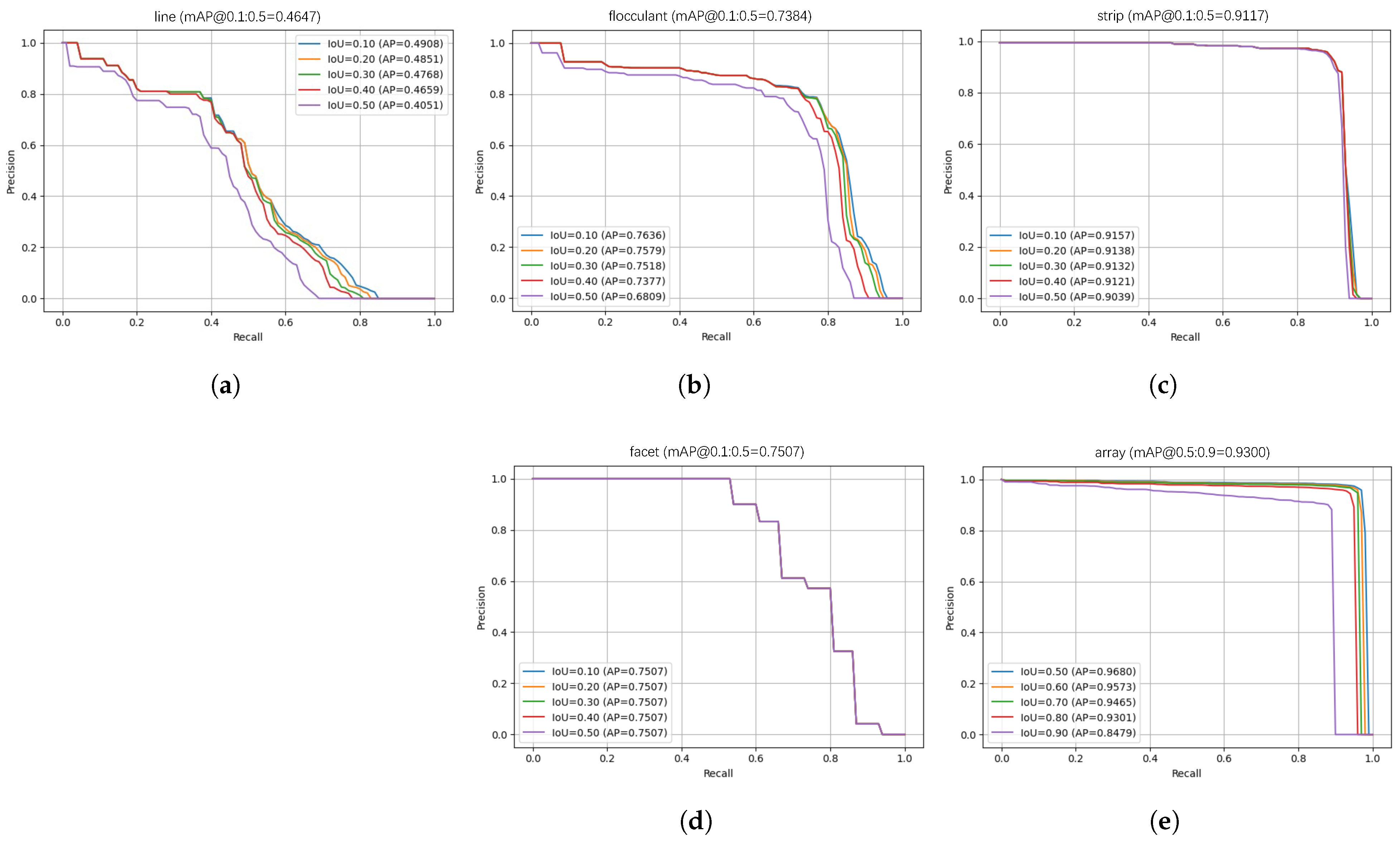
4.3. Quantitative Analysis

To conduct a comprehensive quantitative analysis of the proposed method, we evaluated the precision–recall (PR) curves for various hotspot types and PV arrays under different IoU thresholds, along with derived metrics. Figure 7 presents the PR curves for each hotspot type at varying IoU thresholds, and the corresponding metrics are summarized in

Table 2. Precision and recall metrics of different categories for the proposed detection method.

Categories	Precision@0.1	Precision@0.5	Recall@0.1	Recall@0.5	AP@0.1:0.5	AP@0.5:0.9
Line Hotspot	0.6091	0.5556	0.4900	0.4400	0.4647	0.1650
Flo Hotspot	0.7873	0.7302	0.7700	0.7200	0.7384	0.3697
Strip Hotspot	0.9219	0.9325	0.9000	0.8900	0.9117	0.5665
Facet Hotspot	0.8333	0.8333	0.6600	0.6600	0.7507	0.4930
Average	0.7879	0.7050	0.7629	0.6775	0.7164	0.3986
PV Array	0.9754	0.9671	0.9700	0.9600	0.9773	0.9300

. As shown in Figure 7a, the average precision (AP) for line-shaped hotspots decreases gradually from 0.4908 to 0.4051 as the IoU threshold increases from 0.1 to 0.5. Precision decreases from 0.6091 at IoU = 0.1 to 0.5556 at IoU = 0.5, while recall declines from 0.4900 to 0.4400. These results suggest that line-shaped hotspot detection performs better at lower IoU thresholds, as higher thresholds reduce accuracy due to the complexity of elongated structures. The PR curve for flocculant-shaped hotspots, shown in Figure 7b, exhibits a smoother downward trend, with relatively high AP values across IoU thresholds. AP decreases from 0.7636 at IoU = 0.1 to 0.6809 at IoU = 0.5. Table 2 shows the precision and recall values of 0.7873 and 0.7700, respectively, at IoU = 0.1, outperforming the linear hotspots. These results indicate that the distinctive characteristics of flocculant targets allow the model to detect them more reliably. As shown in Figure 7c, the PR curve for strip-shaped hotspots remains nearly consistent across IoU thresholds, with AP values ranging from 0.9039 to 0.9157. Table 2 shows precision and recall values of 0.9325 and 0.8900, respectively, at IoU = 0.5. The high precision and recall rates for strip-shaped targets are attributed to their geometric regularity, which is easier for the model to capture. The PR curve for facet-shaped hotspots, shown in Figure 7d, demonstrates stable performance, with the AP values remaining consistent at 0.7507 across all IoU thresholds. Table 2 reports the precision and recall values of 0.8333 and 0.6600, respectively, at IoU = 0.1. The weaker performance compared to strip-shaped hotspots can be attributed to the smaller number of facet-shaped hotspot samples (168) in the dataset, compared to 3377 for strip-shaped hotspots. Among the different categories of hotspots, the strip-shaped hotspots achieve the highest detection performance, with AP@0.1:0.5 = 0.9117, significantly outperforming line-shaped (0.4647) and facet-shaped (0.7507) hotspots. In contrast, line-shaped and facet-shaped hotspot detection is more affected by complex backgrounds, target morphology, and sample size.

The PR curve for PV arrays, shown in Figure 7e, highlights stable AP values under higher IoU thresholds (0.5 to 0.9), ranging from 0.8479 to 0.9680. The model achieves exceptional performance, with Precision@0.5 = 0.9671, Recall@0.5 = 0.9600, and AP@0.5:0.9 = 0.9300. These results demonstrate the model’s robustness in detecting PV arrays despite their rotational and morphological diversity. The smoothness of the PR curve further reflects the model’s ability to generalize effectively in complex scenarios, such as deserts and roof areas.

The results demonstrate that the proposed model effectively balances precision and recall across various hotspot types and scenarios, even under the challenges of small target sizes, complex backgrounds, and diverse array rotations. The high detection performance for PV arrays further validates the model’s robustness, adaptability, and generalization ability across diverse environmental conditions.

4.4. Comparative Analysis

To evaluate the advancements of the proposed detection method, Faster R-CNN with RRPN [9] and DiffusionDet with RRPN (DiffusionDet-RRPN) are adopted as baseline methods. Both comparison methods adopt a pre-trained ResNet-50 as the backbone. Faster R-CNN with RRPN predicts rotated bounding boxes for five categories, including four types of hotspot defects and PV arrays. DiffusionDet-RRPN is a two-stage variation of [22], which integrates RRPN into the backbone network. It performs initial binary classification and rotated bounding box regression for PV arrays. Diffusion-based random bounding boxes are generated within proposal regions, which are then fed into a denoising decoder, consistent with the one used in the proposed method.

4.4.1. Qualitative Comparison

DiffusionDet-RRPN predicts bounding boxes for the four hotspot defect types. The detection performance is evaluated through qualitative and quantitative comparisons, as well as model volume and inference efficiency. The qualitative results are illustrated in Figure 8, which demonstrates the detection outcomes for various hotspot defects and PV arrays. In the first row of Figure 8, three line-shaped hotspots are presented. Faster R-CNN fails to detect any of the targets, reflecting its difficulty in identifying small, elongated targets. DiffusionDet-RRPN successfully detects the most prominent line-shaped hotspot in the upper-left corner but fails to detect the other two weaker targets. In contrast, the proposed method accurately detects all three line-shaped targets. The second row contains a flocculant-shaped hotspot. Both DiffusionDet-RRPN (Figure 8(b2)) and the proposed method (Figure 8(c2)) detect the target with precision, while Faster R-CNN (Figure 8(a2)) roughly identifies the defect location but fails to regress the bounding box accurately. The third row presents three strip-shaped hotspots, where Faster R-CNN (Figure 8(a3)) and DiffusionDet-RRPN (Figure 8(b3)) detect only one of the targets. The proposed method, however, correctly detects all three strip-shaped hotspots. Similarly, in the fourth row featuring a facet-shaped hotspot, both DiffusionDet-RRPN (Figure 8(b4)) and the proposed method (Figure 8(c4)) successfully detect the target, whereas Faster R-CNN (Figure 8(a4)) fails.

For PV arrays, Faster R-CNN with RRPN reliably detects regular, non-rotated arrays. However, it struggles with rotated arrays due to its insensitivity to angular variations, leading to significant prediction errors, as shown in Figure 8(a1). In contrast, the proposed method effectively leverages the anchor-free properties of diffusion and the sensitivity of independent detection heads to angular learning, enabling the robust detection of rotated PV arrays with diverse shapes and orientations.

From the qualitative comparison, it is evident that the proposed method outperforms the existing comparative methods in detecting small targets, adapting to complex rotation scenarios, and achieving higher bounding box regression accuracy and robustness.

4.4.2. Quantitative Comparison

Figure 9 illustrates the precision–recall (PR) curves for different hotspot defect types and PV arrays across the various detection methods, with the corresponding average precision (AP) results provided in

Table 3. Comparison of performance metrics for different models and categories.

Categories	Models	AP@0.1:0.5	AP@0.5:0.9
Line Hotspot	Faster RCNN with RRPN	0.1069	0.0114
	DiffusionDet with RRPN	0.3843	0.1242
	Ours	0.4647	0.1650
Flo Hotspot	Faster RCNN with RRPN	0.6456	0.3091
	DiffusionDet with RRPN	0.6851	0.3336
	Ours	0.7384	0.3697
Strip Hotspot	Faster RCNN with RRPN	0.8733	0.5360
	DiffusionDet with RRPN	0.8120	0.4921
	Ours	0.9117	0.5665
Facet Hotspot	Faster RCNN with RRPN	0.2825	0.1495
	DiffusionDet with RRPN	0.6663	0.3365
	Ours	0.7507	0.4930
Average	Faster RCNN with RRPN	0.4618	0.2402
	DiffusionDet with RRPN	0.6523	0.3447
	Ours	0.7164	0.3986
PV Array	Faster RCNN with RRPN	0.8581	0.7782
	DiffusionDet with RRPN	/	/
	Ours	0.9773	0.9300

.

For line-shaped hotspots, the proposed method demonstrates clear superiority, achieving an AP@0.1:0.5 of 0.4647, compared to 0.3843 for DiffusionDet with RRPN and 0.1069 for Faster R-CNN with RRPN. The PR curve in Figure 9a shows that the proposed method effectively detects small line-shaped targets, even at low recall rates, while the performance of the other methods drops significantly under these conditions. This underscores the proposed method’s enhanced capability for modeling small-scale targets. For flocculant-shaped hotspots, the proposed method achieves an AP@0.1:0.5 of 0.7384, surpassing DiffusionDet with RRPN (0.6851) and Faster R-CNN with RRPN (0.6456). The PR curve in Figure 9b indicates that DiffusionDet with RRPN performs second best but experiences a rapid decline in precision at high recall rates. In contrast, Faster R-CNN struggles significantly under these conditions. These results highlight the robustness of the proposed method in detecting targets with fuzzy boundaries and complex backgrounds. For strip-shaped hotspots, the proposed method achieves an AP@0.1:0.5 of 0.9117, outperforming DiffusionDet with RRPN (0.8120) and Faster R-CNN (0.8733). The PR curve in Figure 9c confirms the stability of the proposed method under high recall conditions, demonstrating its ability to effectively capture the geometric features of strip-shaped targets. For facet-shaped hotspots, the proposed method achieves an AP@0.1:0.5 of 0.7507, significantly higher than DiffusionDet with RRPN (0.6663) and Faster R-CNN (0.2825). The PR curve in Figure 9d shows that Faster R-CNN’s performance declines sharply when the recall rate exceeds 0.2, whereas the proposed method and DiffusionDet with RRPN maintain high precision across all recall ranges.

Table 3 summarizes the overall detection performance, showing that the proposed method achieves an average AP@0.1:0.5 of 0.7164, outperforming DiffusionDet with RRPN (0.6523) and Faster R-CNN (0.4618). Additionally, the proposed method achieves an AP@0.5:0.9 of 0.3986, further demonstrating its robustness under stricter IoU conditions, compared to DiffusionDet with RRPN (0.3447) and Faster R-CNN (0.2402). These results emphasize the proposed method’s balanced performance across multiple target types, excelling in small target detection, handling complex backgrounds, and accommodating diverse target shapes.

For PV arrays, DiffusionDet with RRPN fails to detect array regions, leaving the comparison to the proposed method and Faster R-CNN. The proposed method achieves an AP@0.5:0.9 of 0.9300, far exceeding Faster R-CNN’s 0.7782. These advantages are primarily due to the anchor-free diffusion mechanism and the sensitivity of the independent detection heads to angular learning, enabling the precise detection of rotated PV arrays across complex backgrounds.

The model volume and inference efficiency are compared in

Table 4. Comparison of model parameters, inference time, and FPS.

Models	Parameters (M)	Time (s)	FPS
Faster RCNN with RRPN	85.817	0.0833	12
DiffusionDet with RRPN	70.0398	0.0513	19
Ours	111.8674	0.0571	18

. DiffusionDet with RRPN has the lowest parameter number, while Faster R-CNN with RRPN contains 85.817 M parameters. The proposed method has the highest parameter number at 111.8674 M, primarily due to the integration of a more complex diffusion mechanism and independent detection heads. Despite this, the increased parameters contribute to enhanced detection performance. In terms of inference speed, DiffusionDet with RRPN achieves the highest FPS at 19, followed closely by the proposed method at 18 FPS, with Faster R-CNN lagging significantly at 12 FPS. An interesting finding from Table 4 is that our method has more parameters than Faster R-CNN, yet achieves a shorter inference time. This can primarily be attributed to the anchor-free mechanism of our diffusion process. In Faster R-CNN, Region Proposal Networks (RPNs) are used during testing to search for target regions. These networks generate up to 6000 proposals, with 2000 retained after non-maximum suppression (NMS). In contrast, our method only requires 300 proposals to achieve better results. The diffusion mechanism in our approach enables more accurate and efficient proposal generation, leading to higher-quality initial proposals. Furthermore, the diffusion-based anchor-free approach eliminates the need for the exhaustive anchor matching process used in Faster R-CNN, contributing to the faster inference time. These results demonstrate that the proposed method delivers nearly the same inference efficiency as DiffusionDet with RRPN while achieving substantially better detection performance, significantly surpassing Faster R-CNN.

In conclusion, the proposed method strikes a balance between moderate increases in parameter number, efficient inference speed, and superior detection performance. It outperforms the comparative methods across all evaluation metrics, particularly in detecting small targets, handling diverse rotations, and achieving high regression precision under strict IoU thresholds.

5. Discussion

The proposed method effectively addresses the challenges of detecting hotspot defects and PV arrays under varying conditions. Compared to Faster R-CNN with RRPN and DiffusionDet with RRPN, the model demonstrates superior capability in detecting small-scale, rotated, and morphologically diverse targets, particularly in scenarios with complex backgrounds. The integration of diffusion-based rotated bounding boxes enhances sensitivity to angular variations, which is critical for accurate PV array detection. Additionally, the incorporation of the inside-awareness loss function in the defect branch effectively captures the intrinsic relationship between PV arrays and defects, significantly improving detection robustness. Our findings build on prior advancements in PV system defect detection, while extending the state-of-the-art system through the adoption of anchor-free mechanisms and a dual-branch structure. To evaluate the timeliness of our method for large-scale photovoltaic power plants requiring real-time monitoring, we analyzed typical UAV survey operations. According to [4], UAV surveys of large PV plants last 10–20 min and capture 300 to 500 images per flight. Our method processes a single image in 0.057 s on an Nvidia A100 (32 GB) GPU (NVIDIA Corporation, Santa Clara, CA, USA). For a UAV flight capturing 400 images, the total processing time would be around 23 s. This demonstrates that our model can efficiently meet the real-time monitoring demands of large-scale PV plant inspections.

Despite the advantages of our model, certain limitations persist, as illustrated by the failure cases in Figure 10. As shown in Figure 10a, false positives occur when detecting rotating rectangular frames. This issue arises from the angle sensitivity of bounding boxes for incomplete rotating arrays. Due to the irregular shape of incomplete arrays, bounding boxes at different rotation angles may have similar overlap rates with the PV array, leading to multiple predictions (e.g., two bounding boxes in this case). Figure 10b demonstrates a missed detection of a line-shaped hotspot, caused by the relatively low temperature of the hotspot and insufficiently distinct texture features, resulting in low confidence in the model’s prediction. Similarly, Figure 10c shows a missed detection of a flocculant hotspot, which also suffers from weak temperature and texture characteristics. In the same figure, the model misclassifies a strip-shaped hotspot as a facet-shaped hotspot. The large area of the hotspot resembles the typical appearance of a facet-shaped hotspot, making it challenging for the model to differentiate between the two. Figure 10d highlights a false alarm where the model detects a facet-shaped hotspot caused by the sunlit reflection from a PV module. Additionally, in Figure 10e, a missed detection of flocculant hotspots occurs due to their scattered nature, which makes them harder to detect. Despite these challenges, the proposed inside-awareness loss significantly reduces false alarms outside the PV arrays, greatly improving detection accuracy. However, challenges remain in detecting incomplete or small rotated arrays, hotspots with low temperatures, and reflections from PV modules.

In real-world scenarios, UAV flights typically capture images with 30–50% overlap. In the future work, we will explore multi-frame fusion techniques and integrate temporal data from video sequences to the model’s robustness and detectability. Additionally, reducing computational overhead while maintaining detection precision will be a key area for future research.

6. Conclusions

This study presents a dual-branch diffusion detection model for detecting photovoltaic arrays and hotspot defects in infrared images. The model overcomes challenges like small target sizes, diverse rotation angles, and complex backgrounds. Extensive experiments on a comprehensive PV dataset show significant performance improvements, with the method achieving a mean average precision (mAP) of 71.64% for hotspot detection and 97.7% for PV array detection. The model consistently outperforms existing methods in precision and recall across the various defect types and conditions. The model excels at detecting small-scale and rotated objects, with high performance on line-shaped (mAP@0.1:0.5 = 0.4647), flocculant-shaped (mAP@0.1:0.5 = 0.7384), strip-shaped (mAP@0.1:0.5 = 0.9117), and facet-shaped hotspots (mAP@0.1:0.5 = 0.7507). These results emphasize the model’s potential for real-time solar energy management applications. The diffusion-based, anchor-free detection mechanism and inside-awareness loss function further enhance the model’s robustness and adaptability, ensuring strong generalization across different scenarios. In conclusion, the proposed method advances automated photovoltaic monitoring, offering a powerful tool for defect detection in PV arrays, essential for improving the efficiency and safety of solar power plants.

References

1. Čabo, F.G.; Marinić-Kragić, I.; Garma, T.; Nižetić, S. Development of thermo-electrical model of photovoltaic panel under hot-spot conditions with experimental validation. Energy 2021, 230, 120785. [Google Scholar] [CrossRef]
2. Du, B.; Yang, R.; He, Y.; Wang, F.; Huang, S. Nondestructive inspection, testing and evaluation for Si-based, thin film and multi-junction solar cells: An overview. Renew. Sustain. Energy Rev. 2017, 78, 1117–1151. [Google Scholar] [CrossRef]
3. Shengxue, T.; Yue, X.; Li, C.; Xiao, S.; Fang, Y. Study on suppressing strategy of hot spot in solar cell series. Acta Energiae Solaris Sin. 2022, 43, 226. [Google Scholar]
4. Michail, A.; Livera, A.; Tziolis, G.; Candás, J.L.C.; Fernandez, A.; Yudego, E.A.; Martínez, D.F.; Antonopoulos, A.; Tripolitsiotis, A.; Partsinevelos, P.; et al. A comprehensive review of unmanned aerial vehicle-based approaches to support photovoltaic plant diagnosis. Heliyon 2024, 10, e23983. [Google Scholar] [CrossRef] [PubMed]
5. Lofstad-Lie, V.; Marstein, E.S.; Simonsen, A.; Skauli, T. Cost-Effective Flight Strategy for Aerial Thermography Inspection of Photovoltaic Power Plants. IEEE J. Photovolt. 2022, 12, 1543–1549. [Google Scholar] [CrossRef]
6. de Oliveira, A.K.V.; Aghaei, M.; Rüther, R. Automatic Inspection of Photovoltaic Power Plants Using Aerial Infrared Thermography: A Review. Energies 2022, 15, 2055. [Google Scholar] [CrossRef]
7. Dotenco, S.; Dalsass, M.; Winkler, L.; Würzner, T.; Brabec, C.; Maier, A.; Gallwitz, F. Automatic detection and analysis of photovoltaic modules in aerial infrared imagery. In Proceedings of the 2016 IEEE Winter Conference on Applications of Computer Vision (WACV), Lake Placid, NY, USA, 7–10 March 2016; pp. 1–9. [Google Scholar] [CrossRef]
8. Jiang, L.; Su, J.; Li, X. Hot spots detection of operating PV arrays through IR thermal image using method based on curve fitting of gray histogram. Matec Web Conf. 2016, 61, 06017. [Google Scholar] [CrossRef]
9. Ren, S.; He, K.; Girshick, R.; Sun, J. Faster R-CNN: Towards Real-Time Object Detection with Region Proposal Networks. IEEE Trans. Pattern Anal. Mach. Intell. 2017, 39, 1137–1149. [Google Scholar] [CrossRef] [PubMed]
10. Liu, W.; Anguelov, D.; Erhan, D.; Szegedy, C.; Reed, S.; Fu, C.Y.; Berg, A.C. SSD: Single Shot MultiBox Detector. In Proceedings of the Computer Vision—ECCV 2016, Amsterdam, The Netherlands, 11–14 October 2016; Leibe, B., Matas, J., Sebe, N., Welling, M., Eds.; Springer: Cham, Switzerland, 2016; pp. 21–37. [Google Scholar]
11. Terven, J.; Córdova-Esparza, D.M.; Romero-González, J.A. A Comprehensive Review of YOLO Architectures in Computer Vision: From YOLOv1 to YOLOv8 and YOLO-NAS. Mach. Learn. Knowl. Extr. 2023, 5, 1680–1716. [Google Scholar] [CrossRef]
12. Jocher, G.; Stoken, A.; Borovec, J.; Changyu, L.; Hogan, A.; Diaconu, L.; Ingham, F.; Poznanski, J.; Fang, J.; Yu, L.; et al. ultralytics/yolov5: v3. 1-bug fixes and performance improvements. Zenodo 2020. [Google Scholar]
13. Wu, X.; Hao, X. SK-FRCNN: A Fault Detection Method for Hot Spots on Photovoltaic Panels. IEEE Access 2023, 11, 121379–121386. [Google Scholar] [CrossRef]
14. Hao, S.; Li, J.; Ma, X.; Sun, S.; Tian, Z.; Li, T.; Hou, Y. A Photovoltaic Hot-Spot Fault Detection Network for Aerial Images Based on Progressive Transfer Learning and Multiscale Feature Fusion. IEEE Trans. Geosci. Remote Sens. 2024, 62, 4709713. [Google Scholar] [CrossRef]
15. Qian, H.; Shen, W.; Xu, W.S. Hotspot defect detection for photovoltaic modules under complex backgrounds. Multimed. Syst. 2023, 29, 3245–3258. [Google Scholar] [CrossRef]
16. Lei, Y.; Wang, X.; Guan, A.H. Deeplab-YOLO: A method for detecting hot-spot defects in infrared image PV panels by combining segmentation and detection. J. Real-Time Image Process. 2024, 21, 52.1–52.11. [Google Scholar] [CrossRef]
17. Zahradník, D.; Roučka, F.; Karlovská, L. Flat roof classification and leaks detections by Deep Learning. Stavebni Obz.-Civ. Eng. J. 2023, 32. [Google Scholar] [CrossRef]
18. Li, Z.; Zhang, Y.; Wu, H.; Suzuki, S.; Namiki, A.; Wang, W. Design and Application of a UAV Autonomous Inspection System for High-Voltage Power Transmission Lines. Remote Sens. 2023, 15, 865. [Google Scholar] [CrossRef]
19. Mei, B.; Han, R.; Jiang, X.; Wang, Y.; Yin, D. Failure Detection Of Infrared Thermal Imaging Power Equipment Based On Improved DenseNet. In Proceedings of the 2021 14th International Congress on Image and Signal Processing, BioMedical Engineering and Informatics (CISP-BMEI), Shanghai, China, 23–25 October 2021; pp. 1–5. [Google Scholar] [CrossRef]
20. Liao, K.C.; Liou, J.L.; Hidayat, M.; Wen, H.T.; Wu, H.Y. Detection and Analysis of Aircraft Composite Material Structures Using UAV. Inventions 2024, 9, 47. [Google Scholar] [CrossRef]
21. Wyatt, J.; Leach, A.; Schmon, S.M.; Willcocks, C.G. AnoDDPM: Anomaly Detection with Denoising Diffusion Probabilistic Models Using Simplex Noise. In Proceedings of the IEEE/CVF Conference on Computer Vision and Pattern Recognition (CVPR) Workshops, New Orleans, LA, USA, 19–20 June 2022; pp. 650–656. [Google Scholar]
22. Chen, S.; Sun, P.; Song, Y.; Luo, P. DiffusionDet: Diffusion Model for Object Detection. In Proceedings of the IEEE/CVF International Conference on Computer Vision (ICCV), Paris, France, 2–6 October 2023; pp. 19830–19843. [Google Scholar]
23. Nag, S.; Zhu, X.; Deng, J.; Song, Y.Z.; Xiang, T. DiffTAD: Temporal Action Detection with Proposal Denoising Diffusion. In Proceedings of the IEEE/CVF International Conference on Computer Vision (ICCV), Paris, France, 2–6 October 2023; pp. 10362–10374. [Google Scholar]
24. Shi, Y.; Lin, Y.; Wei, P.; Xian, X.; Chen, T.; Lin, L. Diff-Mosaic: Augmenting Realistic Representations in Infrared Small Target Detection via Diffusion Prior. IEEE Trans. Geosci. Remote Sens. 2024, 62, 5004311. [Google Scholar] [CrossRef]
25. Zhou, X.; Hou, J.; Yao, T.; Liang, D.; Liu, Z.; Zou, Z.; Ye, X.; Cheng, J.; Bai, X. Diffusion-Based 3D Object Detection with Random Boxes. In Proceedings of the Pattern Recognition and Computer Vision, Xiamen, China, 13–15 October 2023; Liu, Q., Wang, H., Ma, Z., Zheng, W., Zha, H., Chen, X., Wang, L., Ji, R., Eds.; Springer: Singapore, 2024; pp. 28–40. [Google Scholar]
26. He, T.; Hao, S.; Zhang, X.; Ma, X.; Sun, S.; Yang, C. APM²Det: A Photovoltaic Hot-Spot Fault Detection Network Based on Angle Perception and Model Migration. IEEE Trans. Dielectr. Electr. Insul. 2024, 31, 2938–2946. [Google Scholar] [CrossRef]
27. Wang, D.; Yan, P.; Yao, C.; Xiao, B.; Zhao, W.; Zhu, R. A lightweight joint metric detection approach on YOLO for hot spots in photovoltaic modules. J. Renew. Sustain. Energy 2024, 16, 053503. [Google Scholar] [CrossRef]
28. Tan, H.; Guo, Z.; Zhang, H.; Chen, Q.; Lin, Z.; Chen, Y.; Yan, J. Enhancing PV panel segmentation in remote sensing images with constraint refinement modules. Appl. Energy 2023, 350, 121757. [Google Scholar] [CrossRef]
29. Guo, Z.; Zhuang, Z.; Tan, H.; Liu, Z.; Li, P.; Lin, Z.; Shang, W.L.; Zhang, H.; Yan, J. Accurate and generalizable photovoltaic panel segmentation using deep learning for imbalanced datasets. Renew. Energy 2023, 219, 119471. [Google Scholar] [CrossRef]
30. Ho, J.; Jain, A.; Abbeel, P. Denoising Diffusion Probabilistic Models. In Advances in Neural Information Processing Systems; Larochelle, H., Ranzato, M., Hadsell, R., Balcan, M., Lin, H., Eds.; Curran Associates, Inc.: Red Hook, NY, USA, 2020; Volume 33, pp. 6840–6851. [Google Scholar]
31. Song, J.; Meng, C.; Ermon, S. Denoising Diffusion Implicit Models. arXiv 2022, arXiv:2206.05564. [Google Scholar] [CrossRef]
32. Rombach, R.; Blattmann, A.; Lorenz, D.; Esser, P.; Ommer, B. High-Resolution Image Synthesis With Latent Diffusion Models. In Proceedings of the IEEE/CVF Conference on Computer Vision and Pattern Recognition (CVPR), New Orleans, LA, USA, 18–24 June 2022; pp. 10684–10695. [Google Scholar]
33. Karras, T.; Aittala, M.; Aila, T.; Laine, S. Elucidating the Design Space of Diffusion-Based Generative Models. In Advances in Neural Information Processing Systems; Koyejo, S., Mohamed, S., Agarwal, A., Belgrave, D., Cho, K., Oh, A., Eds.; Curran Associates, Inc.: Red Hook, NY, USA, 2022; Volume 35, pp. 26565–26577. [Google Scholar]
34. Ding, X.; Wang, Y.; Zhang, K.; Wang, Z.J. CCDM: Continuous Conditional Diffusion Models for Image Generation. arXiv 2024, arXiv:22405.03546. [Google Scholar] [CrossRef]
35. Rezatofighi, H.; Tsoi, N.; Gwak, J.; Sadeghian, A.; Reid, I.; Savarese, S. Generalized Intersection Over Union: A Metric and a Loss for Bounding Box Regression. In Proceedings of the IEEE/CVF Conference on Computer Vision and Pattern Recognition (CVPR), Long Beach, CA, USA, 15–20 June 2019. [Google Scholar]
36. Russell, B.C.; Torralba, A.; Murphy, K.P.; Freeman, W.T. LabelMe: A Database and Web-Based Tool for Image Annotation. Int. J. Comput. Vis. 2008, 77, 157–173. [Google Scholar] [CrossRef]
Figure 1. Representative infrared images of PV arrays and hotspots. (ad) indicate four different types of PV hotspots: line-shaped, flocculant-shaped, strip-shaped, and facet-shaped defects. (e) shows rotated PV arrays. (f) shows PV arrays occluded by trees.
Remotesensing 17 01084 g001
Figure 3. The framework of the proposed dual-branch photovoltaic diagnostic network.
Remotesensing 17 01084 g003
Figure 4. The diffusion process and RROI pooler of the array branch. The rotation angle α is determined by rotating the rectangle counterclockwise, aligning the longer side w with the x-axis for the first time.
Remotesensing 17 01084 g004
Figure 5. Diagrams of the proposed inside-awareness loss. (a) Convex hull of two rectangles. IoU, IIoU, UoC, and L inside defined by (6) for cases of (b) proposal box B ^ D inside the array box B A , (c) proposal box B ^ D outside the array box B A , (d) proposal box B ^ D interacting with the array box B A . Larger IoU, IIoU, and UoC indicate better instances, while a larger L inside means worse cases.
Remotesensing 17 01084 g005
Figure 6. Representative photovoltaic (PV) array and hotspot defect detection results are shown for different PV power station scenarios, including water, roof, and ground installations. The images illustrate various hotspot defect shapes, including (a1a3) line-shaped hotspots, (b1b3) flocculant-shaped hotspots, (c1c3) strip-shaped hotspots, and (d1d3) facet-shaped hotspots. The percentage around the text label represents the detection score.
Remotesensing 17 01084 g006
Figure 7. Precision–recall (PR) curves of different IoU thresholds derived by the proposed detection method. (a) PR curves of the line-shaped defect. (b) PR curves of the flocculant-shaped defect. (c) PR curves of the strip-shaped defect. (d) PR curves of the facet-shaped defect. (e) PR curves of the PV array. AP indicates the area under the PR curve, and mAP indicates the average AP results for different IoU thresholds.
Remotesensing 17 01084 g007
Figure 8. Visualization comparison for different models. The four rows demonstrate line-shaped, flocculant-shaped, strip-shaped, and facet-shaped hotspot detection performance, successively. (ac), are the output results from the Faster R-CNN with RRPN, DiffusionDet with RRPN, and our model, respectively.
Remotesensing 17 01084 g008
Figure 9. Precision–recall (PR) curves of different objects with specific IoU thresholds derived by the different detection models. (a) PR curves of the line-shaped defect. (b) PR curves of the flocculant-shaped defect. (c) PR curves of the strip-shaped defect. (d) PR curves of the facet-shaped defect. (e) PR curves of the PV array. AP indicates the area under the PR curve.
Remotesensing 17 01084 g009
Figure 10. Failure cases of the proposed method. (a) False negative of rotated array detection. (b) False negative of line-shaped hotspot. (c) False negative of flocculant-shaped hotspot and miss classification. (d) False negative of facet hotspot. (e) False negative of flocculant hotspot.
Remotesensing 17 01084 g010