Abstract
Sparse Synthetic Aperture Radar (SAR) imaging has garnered significant attention due to its ability to suppress azimuth ambiguity in under-sampled conditions, making it particularly useful for high-resolution wide-swath (HRWS) SAR systems. Traditional compressed sensing-based sparse SAR imaging algorithms are hindered by range–azimuth coupling induced by range cell migration (RCM), which results in high computational cost and limits their applicability to large-scale imaging scenarios. To address this challenge, the approximated observation-based sparse SAR imaging algorithm was developed, which decouples the range and azimuth directions, significantly reducing computational and temporal complexities to match the performance of conventional matched filtering algorithms. However, this method requires iterative processing and manual adjustment of parameters. In this paper, we propose a novel deep neural network-based sparse SAR imaging method, namely the Self-supervised Azimuth Ambiguity Suppression Network (SAAS-Net). Unlike traditional iterative algorithms, SAAS-Net directly learns the parameters from data, eliminating the need for manual tuning. This approach not only improves imaging quality but also accelerates the imaging process. Additionally, SAAS-Net retains the core advantage of sparse SAR imaging—azimuth ambiguity suppression in under-sampling conditions. The method introduces self-supervision to achieve orientation ambiguity suppression without altering the hardware architecture. Simulations and real data experiments using Gaofen-3 validate the effectiveness and superiority of the proposed approach.
1. Introduction
High-resolution synthetic aperture radar (SAR) imaging algorithms have recently earned significant attention in the field of SAR imaging. However, due to the constraints imposed by the Nyquist sampling theorem [1], achieving high-resolution wide-format imaging requires higher sampling rates. The SAR imaging problem, viewed as an inverse problem, can potentially overcome this limitation through the application of compressed sensing theory [2,3]. The first proposed application of compressed sensing theory to SAR imaging algorithms was made by [4]. Subsequent work by [5,6,7] further enhanced sparse synthetic aperture radar algorithms. Additionally, compressed sensing algorithms have been applied in the fields of inverse synthetic aperture radar imaging [8,9] and three-dimensional imaging [10,11,12]. Compared to traditional SAR imaging methods, sparse SAR imaging algorithms can reduce the number of samples. However, most of these algorithms operate in the time domain, overlooking or failing to account for azimuth–distance coupling. As a result, they suffer from high computational complexity and memory usage, making them challenging to apply to large-scale scenes or wide-format imaging. Reference [13] proposed an approximated observation-based sparse SAR imaging algorithm that can significantly reduce computational and temporal complexities. This approach maintains consistency in computational complexity and matched filtering algorithms.
In practice, traditional sparse synthetic aperture radar imaging algorithms often require manual parameter tuning. This means that the parameters must be readjusted for different imaging scenarios, and the entire tuning process is heavily reliant on manual experience. In recent years, SAR imaging based on deep learning has been widely used [14,15,16,17,18], leveraging deep learning for adaptive parameter adjustment. Reference [19] introduced the concept of a sparse unfolding network by leveraging the properties of neural networks. This method replaces the iterative process of the original algorithm with a multi-layer neural network, which is used to automatically train and adjust the parameters that would traditionally need manual fine-tuning, ensuring that the parameters are selected optimally. In recent years, deep unfolding networks have found applications in sparse synthetic aperture radar imaging. In [20], a joint range migration and sparse reconstruction network for 3D millimeter-wave imaging was introduced. In [15,21], a SAR imaging framework based on the depth-expanded network of ISTA was proposed and successfully applied to passive SAR. However, these methods are limited in their ability to effectively utilize the structural information inherent in SAR signals and therefore cannot address issues such as range ambiguity and azimuth ambiguity.
Since the energy of azimuth ambiguity cannot be ignored in practical applications, it is essential to pay attention to azimuth ambiguity suppression in sparse SAR imaging. Existing ambiguity suppression algorithms can be broadly categorized into three types: those that directly or indirectly utilize the filtering results of filters [22,23], sparse reconstruction-based algorithms [24,25,26], and those that use regions with less ambiguity for imaging [27,28]. Whether the filter results are directly applied to imaging or used as part of the a priori knowledge, accurate spectral information is critical. Although filtering can effectively mitigate spectral aliasing in certain regions, it often leads to adverse effects on the spectrum in the primary region as well. Sparse reconstruction-based methods, on the other hand, typically involve complex, large-scale computations. These approaches often require manual parameter tuning, making them highly sensitive to user input and limiting their adaptability. Due to the inherent characteristics of radar system imaging, identifying regions with minimal ambiguity proves to be a challenging task. Consequently, the practical implementation of algorithms that rely on these less ambiguous regions for imaging faces substantial obstacles.
Based on this, in this paper, we investigate the cause of azimuthal ambiguity and introduce group sparse constraints to reformulate the SAR imaging model. We employ the compressed sensing algorithm for sparse reconstruction and leverage a network structure to train the parameters that would typically require manual adjustment, significantly mitigating the issue of insufficiently accurate manual tuning. Additionally, a self-supervised algorithm is introduced to address the problem of traditional neural network-based imaging algorithms being overly dependent on existing datasets. The entire algorithm is built upon the chirp scaling algorithm. This choice is motivated by the fact that, under the assumption of a small oblique viewing angle, the chirp scaling algorithm can perform range migration correction more accurately through phase multiplication, rather than interpolation. This is in contrast to the distance Doppler algorithm, which relies on interpolation to handle range migration in the distance–time–azimuth–frequency domain (distance Doppler domain). While the Omega-K algorithm can provide more precise results, it demands more computational resources and is not suitable for large-scale scene imaging [29].
The main contributions of this article are as follows:
(1) Sparse expansion of the iterative process: The iterative process of traditional algorithms is sparsely expanded, and a deep unfolded network is introduced for adaptive training of parameters. This approach addresses the challenges of large computational load, slow processing speed, and poor generalization inherent in traditional algorithms.
(2) Self-supervised imaging network: A self-supervised imaging network structure is designed to tackle the problem of insufficient datasets. This network eliminates the need for manual parameter adjustments and enhances the network’s adaptability to different imaging scenes.
(3) Structural sparsity for azimuthal ambiguity suppression: The concept of structural sparsity is introduced, and the lq-norm is applied for azimuthal ambiguity suppression, leading to further improvements in imaging quality. A joint loss function, combining structural sparsity and principal view clarity, is formulated to achieve azimuthal ambiguity suppression while maintaining robustness against noise.
This method is evaluated using both simulated point targets and real datasets. The experimental results highlight the effectiveness of the algorithm in reducing side-lobes and enhancing target features, demonstrating its potential for tackling challenges in large-scale imaging scenarios.
2. Materials and Methods
In this section, we will first introduce the signal model of sparse SAR imaging, then the novel azimuth ambiguity suppression imaging model will be established. Finally, both the basic Iterative Shrinkage Thresholding Algorithm Net (ISTA-Net) and the Azimuth Ambiguity Suppression Network (AAS-Net), as well as the Self-supervised Azimuth Ambiguity Suppression Network (SAAS-Net), will be introduced.
2.1. Signal Model
The sparsity of a signal refers to the presence of many components that are nearly zero in some representation. In such cases, signal reconstruction can be achieved at a sampling rate much lower than that dictated by the Nyquist sampling theorem, using techniques like compressed sensing [2,3].
2.1.1. Sparse SAR Imaging Model
Given that represents the scattering coefficient of the observation scene, represents the echo signal, represents the observation matrix, and n represents the noise signal, the imaging model of sparse SAR can be expressed as follows:
Essentially, the sparse SAR imaging process is a classic inverse problem that can be solved by compressed sensing methods. Within the compressed sensing framework, the sparse SAR imaging problem can be rewritten as a regularized expression:
In (2), is a regularization parameter that determines by the sparsity of the imaging scene.
As a convex relaxation, the -norm optimization problem can be approximated via -norm optimization as follows:
This optimization problem, with the form of least absolute shrinkage and selection operator (LASSO), can be solved using the Iterative Shrinkage-Thresholding Algorithm (ISTA). In this optimization system, the parameter is always determined by artificial setting based on the sparsity of the imaging scene. The iterative expression is as follows:
In (4), and are regularization parameters, is the scattering coefficient of the observation scene, is the echo signal, and is the observation matrix.
2.1.2. Azimuth Ambiguity Suppression Signal Model
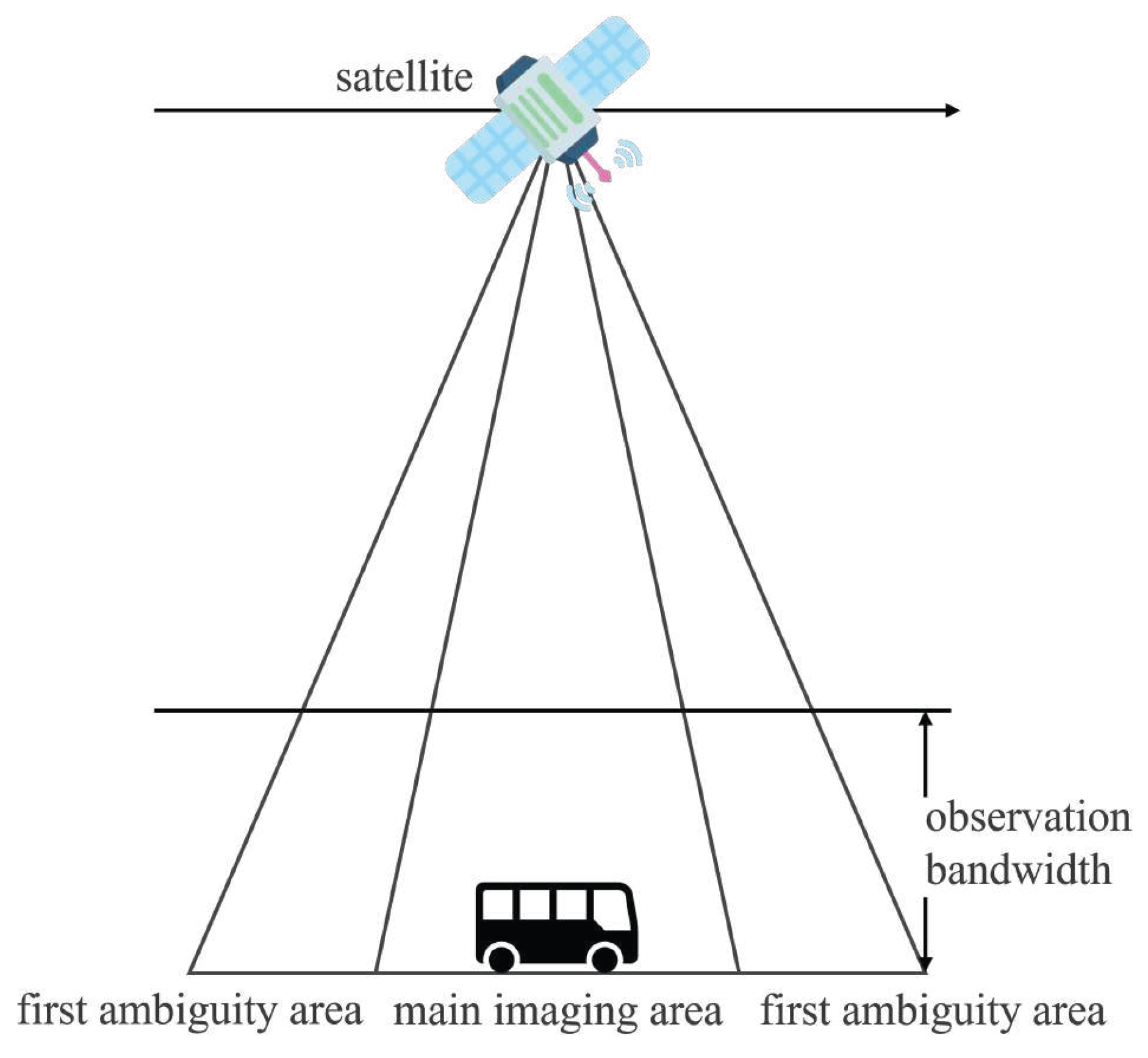
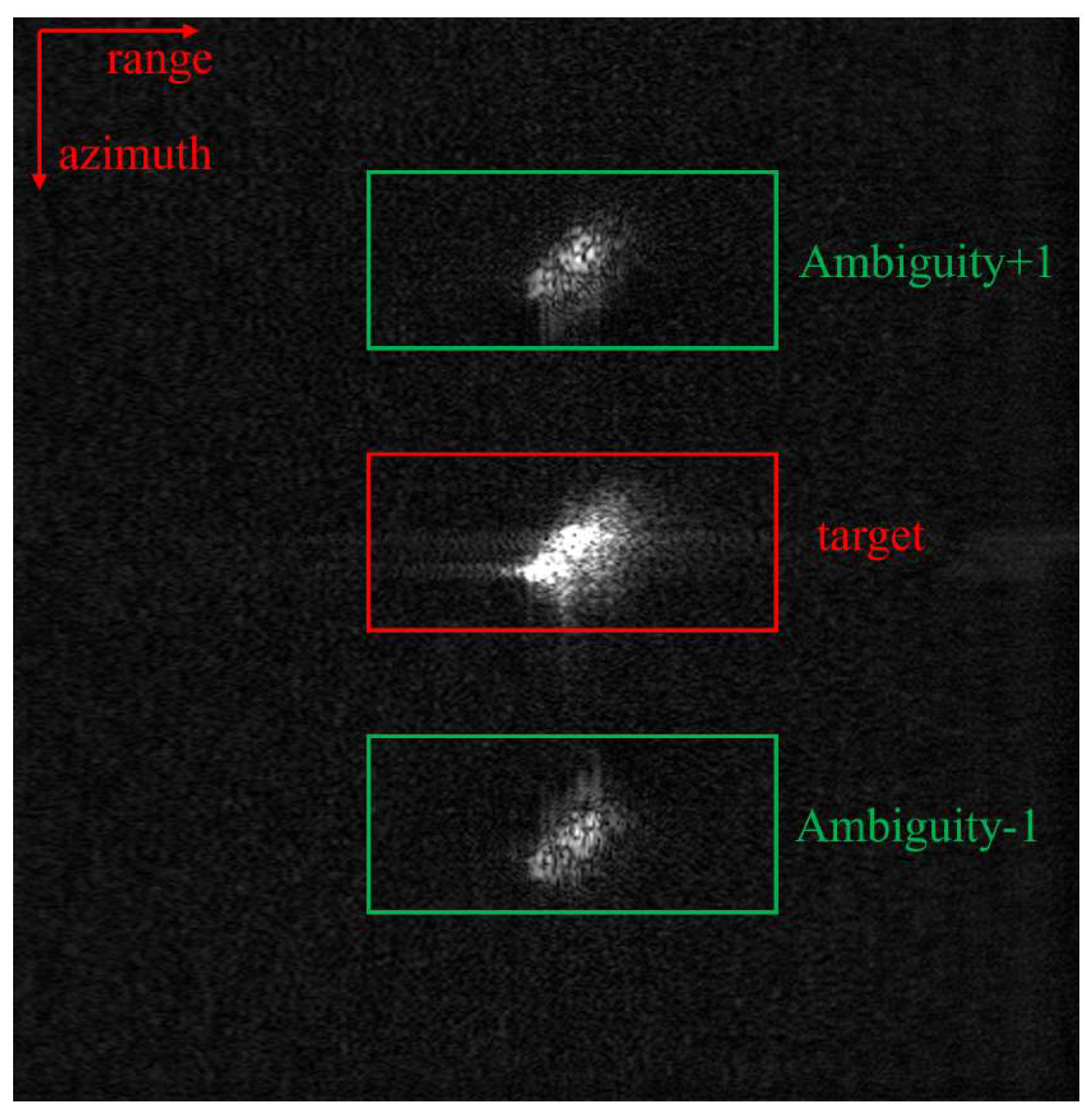
Figure 1 shows the imaging process and illustrates the division between the main region and the ambiguity region. In practice, undersampling in the azimuthal direction often results in ambiguous energy, leading to azimuthal ambiguity. Figure 2 shows a scene with azimuth ambiguity, where a real ship is present in the center region, while the upper and lower parts display artifacts of the ship caused by azimuth ambiguity, which do not actually exist. To address this issue, we introduce group sparsity.

Figure 1.
Diagram of the imaging process.
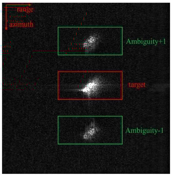
Figure 2.
Azimuth ambiguity diagram.
Sampling in the azimuth direction tends to be non-uniform compared to the range direction, making it more prone to undersampling at certain beam locations. This non-uniform sampling can lead to spectral aliasing in the azimuth direction, resulting in azimuth ambiguity. The azimuth PRF and image width are interdependent because the azimuth resolution improves with a higher PRF, which shortens the time between successive pulses and allows for finer angular separation. However, increasing the image width requires a lower PRF to avoid aliasing, which results in a reduced azimuth resolution, as fewer pulses are transmitted within the same time frame to cover the larger area. Thus, enhancing both parameters simultaneously is not feasible due to this trade-off. Therefore, to achieve high-resolution wide-area imaging, it is crucial to explore techniques for mitigating azimuth ambiguity. Specifically, for the imaging system, the azimuth pulse repetition frequency (PRF) is slightly lower than the minimum PRF required for uniform sampling at certain beam positions, leading to azimuth undersampling and, consequently, azimuth ambiguity in the resulting images.
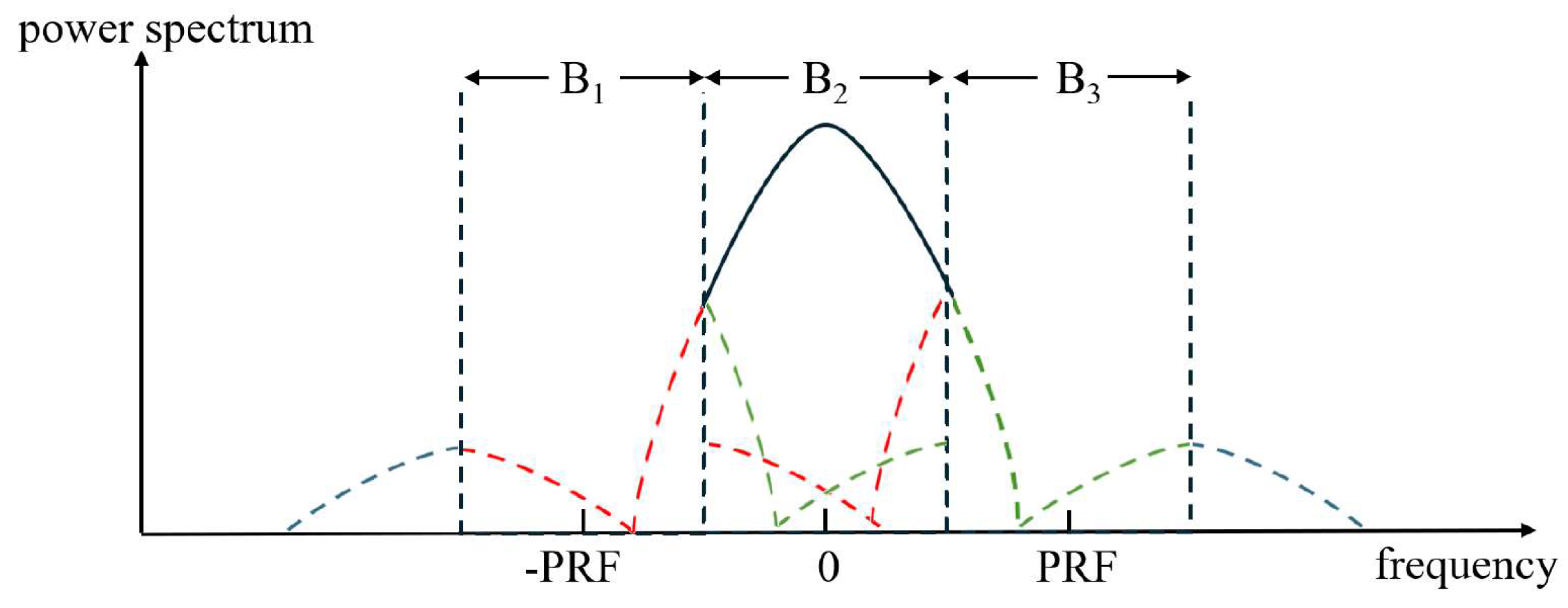
During sparse SAR imaging, the portion of the Doppler spectrum that exceeds the PRF is folded into the azimuth processing bandwidth, causing it to mix with the main signal and resulting in azimuth ambiguity. As shown in Figure 3, the green and red dotted lines illustrate how the ambiguity areas fold into the main area. That is to say that the finite number of samples in the azimuth direction leads to spectral aliasing in the azimuth direction, resulting in azimuth ambiguity. The structure of the SAR imaging operator in the ambiguous regions closely resembles that in the main area, except the azimuth frequency. This means we can use different scattering coefficients to represent signals from different parts. If each set of data is considered as echo data from different angles, then the entire signal model can be expressed as follows:
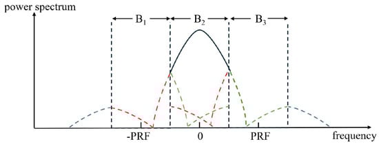
Figure 3.
Schematic of azimuthal frequency spectrum aliasing.
In (5), represents the signal echo as the sparse imaging model. represents the image data from different angles. When , the signal model is the same as the traditional signal model, which means that when , the signal can be seen as the primary view. Furthermore, other parts can be seen as an expanded view. is the observation matrix.
Although the phase and amplitude of the primary and expanded view components of the target may be different, they are always at the same location in the scene. Thus, group sparsity can be utilized to portray this sparsity, introducing the group sparsity constraint. The optimization problem, when constrained by both group sparse constraints and -norm constraints, can be formulated as follows:
Just as for the basic signal model, this optimization problem can be approximated by a -norm optimization:
where represents the group sparsity constraint when indicates signal weights and . The regularization contains two constraint terms. The first one is the group sparsity constraint, and the other is the enhancement of the penalty term for subjective sparsity for suppressing residual ambiguity energy. According to [13], it can also be solved using the ISTA as the basic signal model.
2.2. Method
Based on the sparse SAR signal model proposed in the previous section, in this section, we construct sparse SAR imaging networks using a deep unfolding network, including three types of imaging networks: ISTA-Net, AAS-Net, and SAAS-Net. At the same time, to facilitate comprehension, we also provide an introduction to the corresponding traditional iterative imaging algorithms, namely CS-IST and CS-IST-AAS.
2.2.1. Iterative Shrinkage Thresholding Algorithm Net (ISTA-Net)
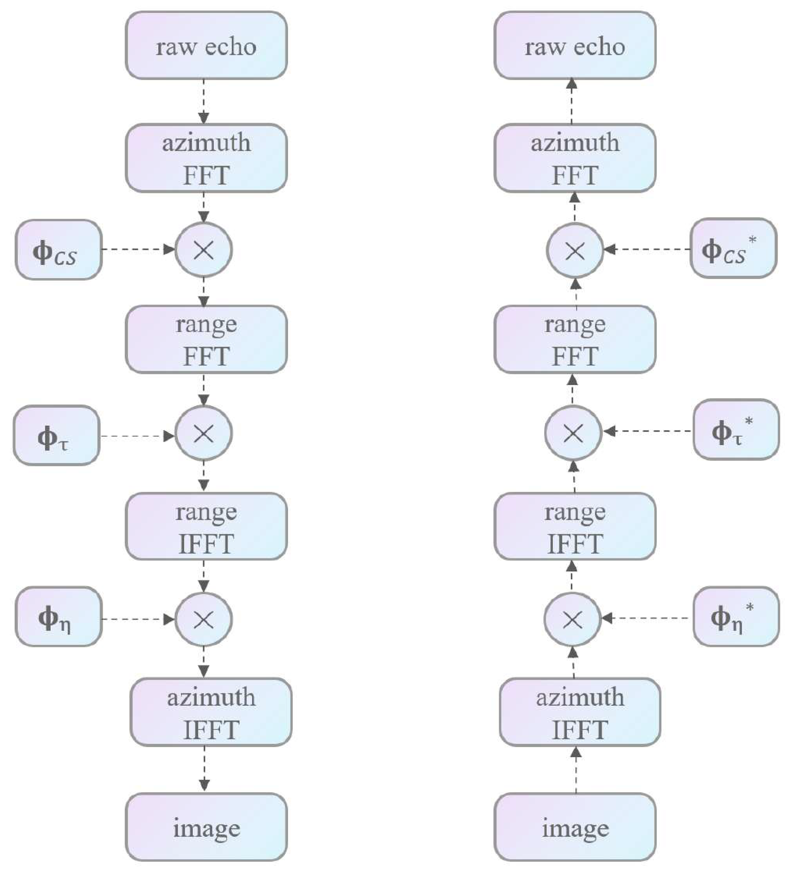
We use I to denote the imaging process of the chirp-scaling (CS) algorithm [30]. Obviously, each step of the CS imaging process is a one-dimensional linear algorithm, so the whole process of CS imaging can be regarded as a series of combinations of one-dimensional steps. These steps can be expressed by the following expression:
where represents the FFT operation in the azimuth direction, represents the FFT operation in the range direction, represents the IFFT operation in the azimuth direction, and represents the IFFT operation in the range direction. represents the range cell migration correction (RCMC) phase term, represents the range compression phase term, and represents the azimuth–range decoupling phase term. Matrices marked with asterisks represent their inverse matrices.
The CS imaging inverse process expression has a similar form, in which G represents the inverse algorithm of the imaging process, which is called the echo simulation operator. The structures of the I and G operators are shown in Figure 4, and G can be expressed as follows:
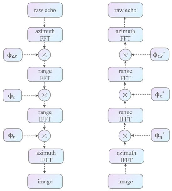
Figure 4.
The structure of the echo simulation operator.
Since each step in the imaging process is a one-dimensional linear algorithm, every imaging step can be represented by matrix multiplication. In other words, the entire imaging process can be expressed as a series of matrix multiplications. If matrix and are used to represent the product of these matrices, then the imaging result and the echo signal should satisfy the following relationship:
At this point, the relationship between the echo signal and the imaging is successfully established through the sparse observation matrix. As a convex optimization problem, it can be solved using the Iterative Shrinkage-Thresholding Algorithm (ISTA). Because we use the ISTA and chirp-scaling algorithm, we call this algorithm CS-IST. The iterative formula is as follows:
where and are the regularization parameters, is the scattering coefficient of the observation scene, is the echo signal, is the inverse algorithm matrix of the imaging process, and is the algorithm matrix of the imaging process.
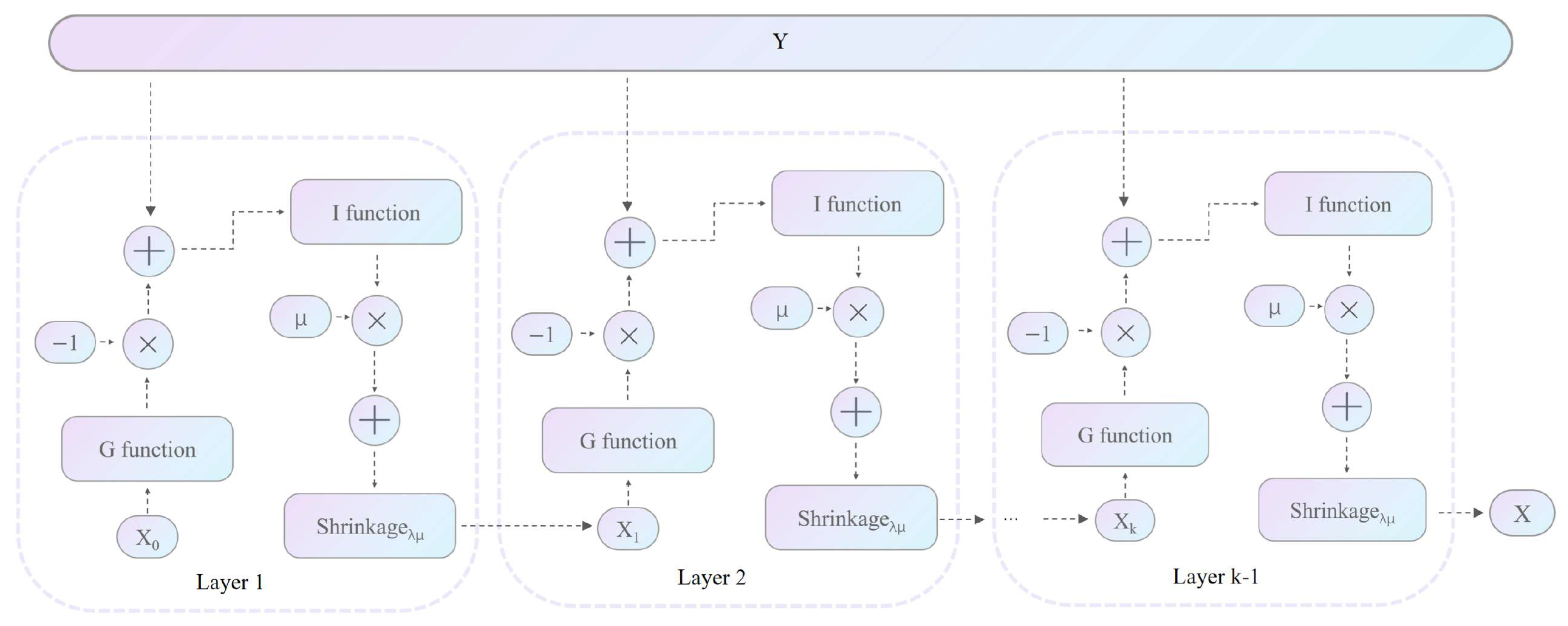
It is obvious that the two parameters, step size and threshold , need to be manually adjusted, and the results of these parameters have a great impact on the experimental results. Therefore, it is considered to utilize the design of a network structure to train these two parameters [13], which ensures that these two parameters are unified in each layer and are adaptively trained between different layers of the network. Because of the use of ISTA, we call this network ISTA-Net. The structure of ISTA-Net is shown in Figure 5.
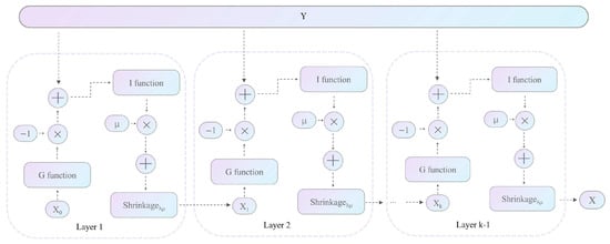
Figure 5.
The iterative process of ISTA-Net.
2.2.2. Azimuth Ambiguity Suppression Network (AAS-Net)
The ambiguity component in the azimuthal direction can be considered as another signal with different observation angles. As a result, the overall signal model at this point can be viewed as a superposition of the ambiguity component and the dominant visual component. In this case, the ambiguity component and the dominant visual component have the same energy distribution, meaning that both the ambiguity solution and the non-ambiguity solution will appear at the same position in the sparse SAR imaging process, with the only difference being the amplitudes of the signals. Therefore, group sparsity can be used to characterize the relationship between the ambiguity and non-ambiguity solutions. At this stage, the number of ambiguous solutions corresponds to the number of ghost images, while the number of non-ambiguous solutions matches the group sparsity. This sparsity is crucial for suppressing azimuthal ambiguity.
According to Formula (6) in the signal model section, if , then the azimuth ambiguity suppression regularization problem mentioned before can be rewritten as a typical sparse regularization problem:
It is obvious that this is a convex problem, and we can use the Fast Iterative Shrinkage Thresholding Algorithm (FISTA) to solve this problem. We call this algorithm CS-IST-AAS based on the use of chirp scaling, the iterative shrinkage thresholding algorithm, and the azimuth ambiguity suppression algorithm. Given , we can use Algorithm 1 to depict this process. represents the residual, U represents the gradient direction, t is the FISTA iteration parameters, is the image signal, and is the intermediate variable of the FISTA algorithm. and are manually adjusted parameters.
| Algorithm 1 CS-ISTA-AAS—Algorithm of chirp scaling-iterative shrinkage thresholding algorithm—azimuth ambiguity suppression. |
| Input: SAR echo signal y, regularization parameter and |
| Output: primary image |
| Initial: , , |
| For: to |
| Update residuals: |
| Update gradient direction: |
| Main view area iteration: |
| Group sparsity iteration: |
| Update parameter: |
| Update intermediate variable: |
| End |
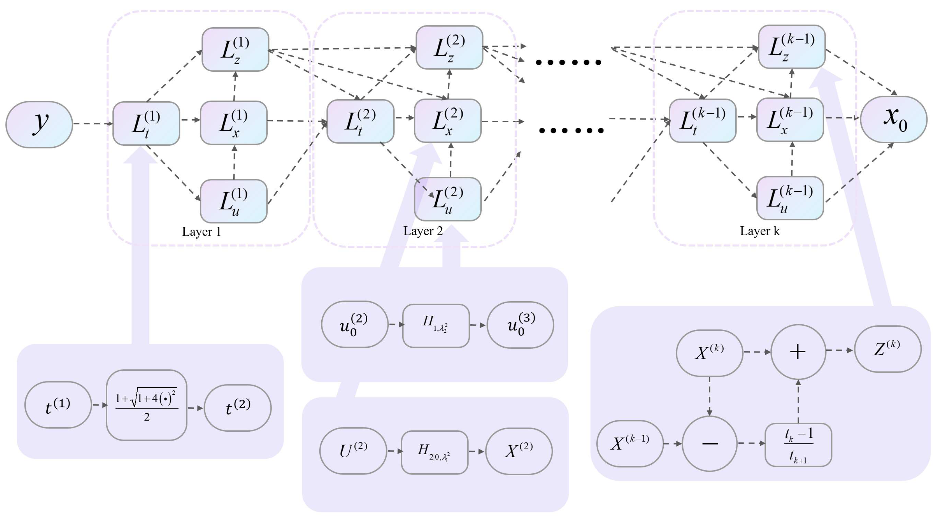
Similar to the basic network, we can use a deep unfolded network to train these parameters. The structure of the unfolded network is shown in Figure 6. We call this network the Azimuth Ambiguity Suppression Network (AAS-Net). For ease of representation, we divide the entire network structure into four modules, , , , and , which are used to update the parameter t, the principal view , the gradient , and the intermediate variable .
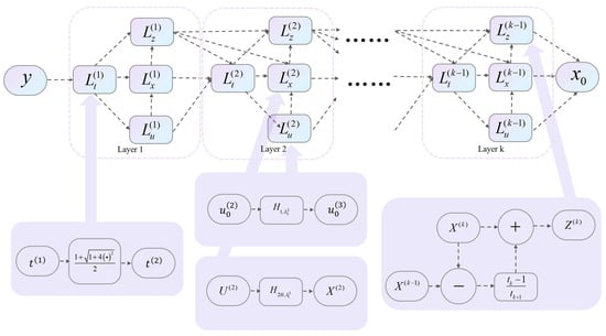
Figure 6.
The iterative process of AAS-Net.
2.2.3. Self-Supervised Azimuth Ambiguity Suppression Network (SAAS-Net)
In practical applications, there is often an insufficient amount of data to support the training process. Additionally, different imaging scenes typically exhibit varying levels of scene sparsity, which requires adjusting iteration parameters accordingly. Therefore, it is essential to design self-supervised imaging networks to address these challenges. In this section, we establish a self-supervised azimuth ambiguity suppression network, and we call it SAAS-Net.
As shown in Figure 7, we design an encoder–decoder network to enable the self-supervised operation of the entire unfolding network. In the encoder, the raw echo signal is partitioned into L smaller echoes. Three of these raw echoes are randomly selected to generate the corresponding reference imaging results, which serve as labels for training the network. The network model is trained using these three sets of reference echoes and their corresponding reference imaging results. In the decoder, the partitioned raw echo signals are processed through the encoder-trained network model to obtain small-area imaging results for each chunk. These imaging results are then stitched together to form the complete large-area imaging output from the decoder. It is noteworthy that within the decoder section, a branch connection is incorporated. This connection directly feeds the echo signal from the encoder input segment into the decoder input, ensuring the seamless progression of the imaging process.
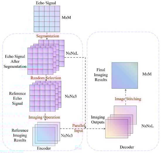
Figure 7.
The structure of SAAS-Net.
The loss function of this network consists of a composite regularization term:
In (15), is main view regularization, which is MSE loss, and is group sparsity regularization. is a regulation parameter. We chose the MSE loss function over the loss function because it generally provides faster convergence and better stability during training due to its smoothness and continuous gradients. The whole loss function is a linear combination of the main view regularization and group sparsity regularization. By using this joint loss function, azimuth ambiguity can be effectively suppressed.
3. Results
In this chapter, we analyze the performance of the SAAS-Net on point target simulation experiments and real data experiments. Since the proposed imaging network is formed by sparse SAR imaging based on ISTA with the chirp-scaling operator, we compare our network with CS-IST, ISTA-Net, and CS-IST-AAS.
3.1. Simulation Experiments and Results
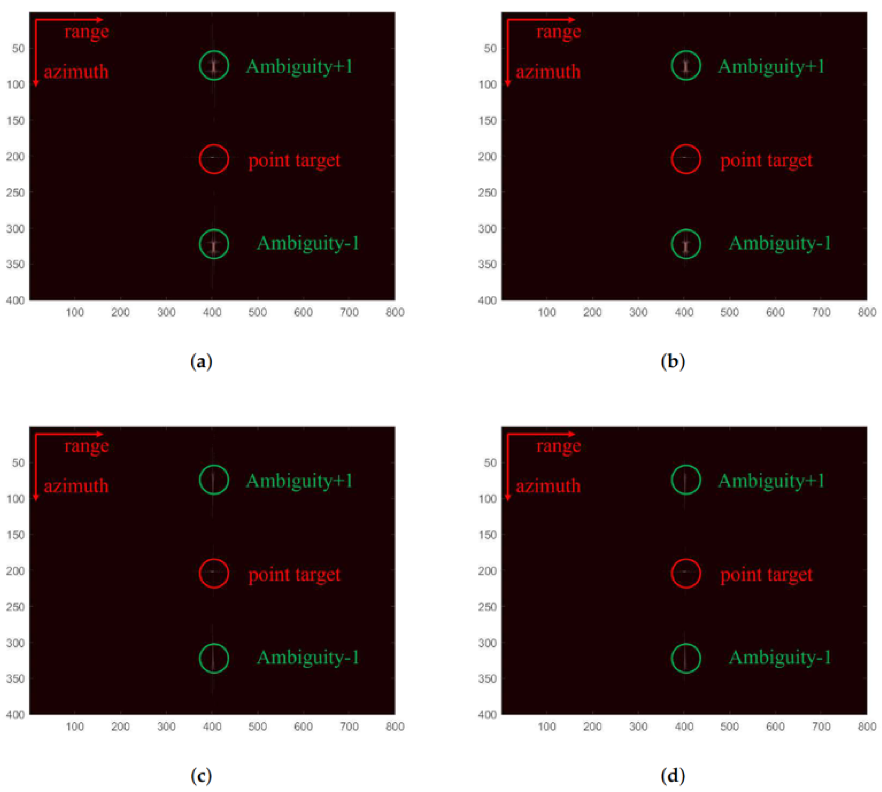
We designed a point-target simulation experiment to test the effectiveness of the network proposed in this paper in terms of orientation ambiguity suppression. Table 1 shows the necessary radar imaging parameters for the simulation experiment, where there is 60% undersampling in the azimuth direction. We used the CS-IST algorithm, CS-IST-AAS algorithm, ISTA-Net, and SAAS-Net for point target imaging. The imaging results are shown in Figure 8.

Table 1.
Parameter values of the simulation experiment.

Figure 8.
Point target imaging results: (a) CS-IST algorithm; (b) ISTA-Net; (c) CS-IST-AAS algorithm; (d) SAAS-Net.
In the imaging results, the longitudinal direction is the azimuthal direction, and the transverse direction is the range direction. In contrast, the ISTA-Net algorithm in Figure 8b can weaken the azimuth ambiguity to a certain degree. The ambiguity phenomenon is eliminated in Figure 8c,d. Comparing Figure 8a to Figure 8b, since Figure 8b uses a deep unfolding network with the theoretically optimal parameters, the imaging result is better than in Figure 8a, which completely relies on manual parameter tuning. Similarly, the imaging result of Figure 8d is slightly better than Figure 8c. At the same time, the algorithms in Figure 8c,d add structural sparsity constraints, and from the perspective of the signal model and the causes of azimuth ambiguity, they suppress azimuth ambiguity. Therefore, compared to the algorithms in Figure 8a,b, they show a significant suppression effect on azimuth ambiguity.
This indicates that SAAS-Net can significantly reduce the side-lobes, which leads to the more accurate reconstruct results. And, the proposed network has better azimuth ambiguity suppression capabilities.
For quantitative comparison, a Monte Carlo experiment was conducted, and the Peak Side-Lobe Ratio (PSNR), Integral Side-Lobe Ratio (ISLR), and mean Azimuth Ambiguity Signal Ratio (AASR) along the azimuth detection were used to evaluate the imaging quality. The formulae for these evaluation parameters are given below. The results are shown in Table 2.
Table 2.
Numerical results of the point target simulation experiment.
Here, A represents the amplitude and S represents the amplitude spectrum.
Monte Carlo experiments further demonstrate the effectiveness of the ambiguity suppression algorithm proposed in this paper for azimuthal ambiguity suppression. In addition, utilizing the unfolding network training, the imaging quality is higher than that of the traditional algorithm because better iteration parameters can be obtained.
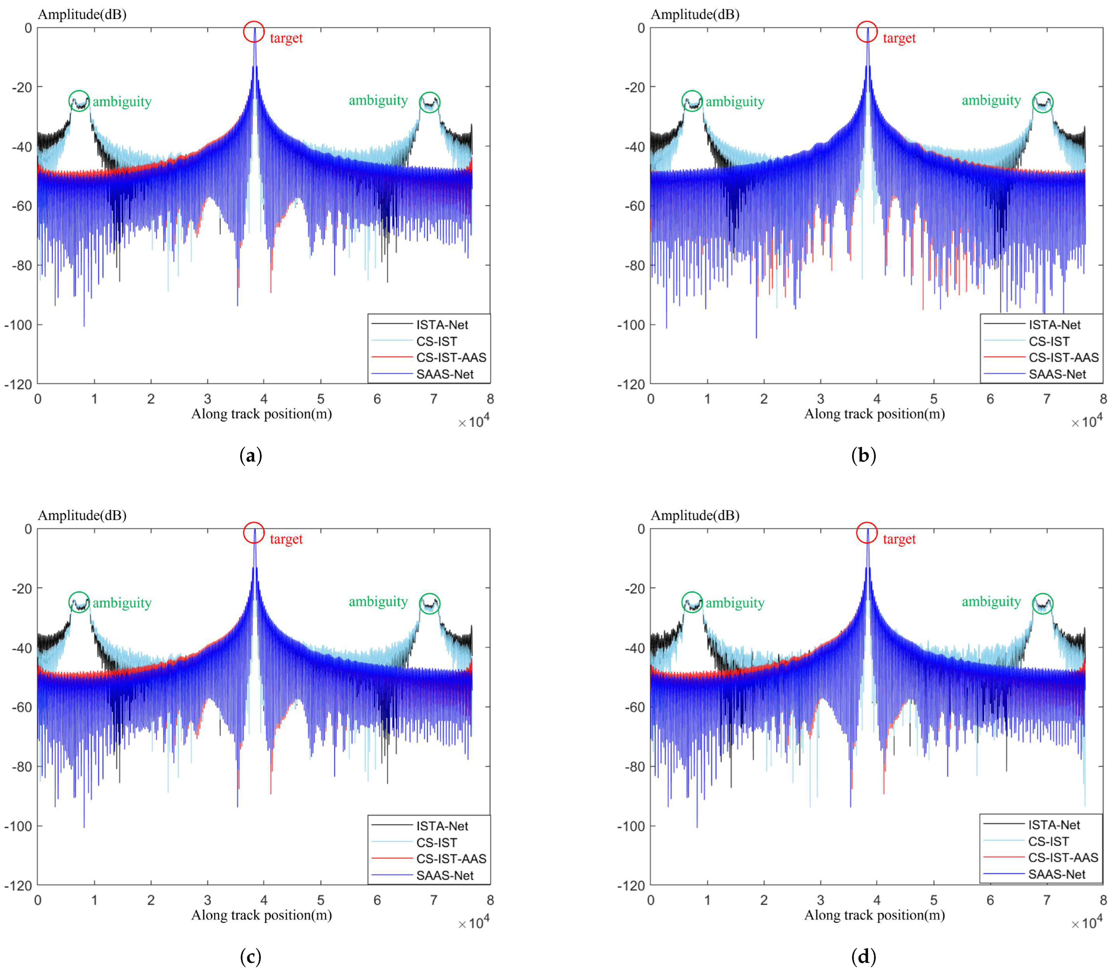
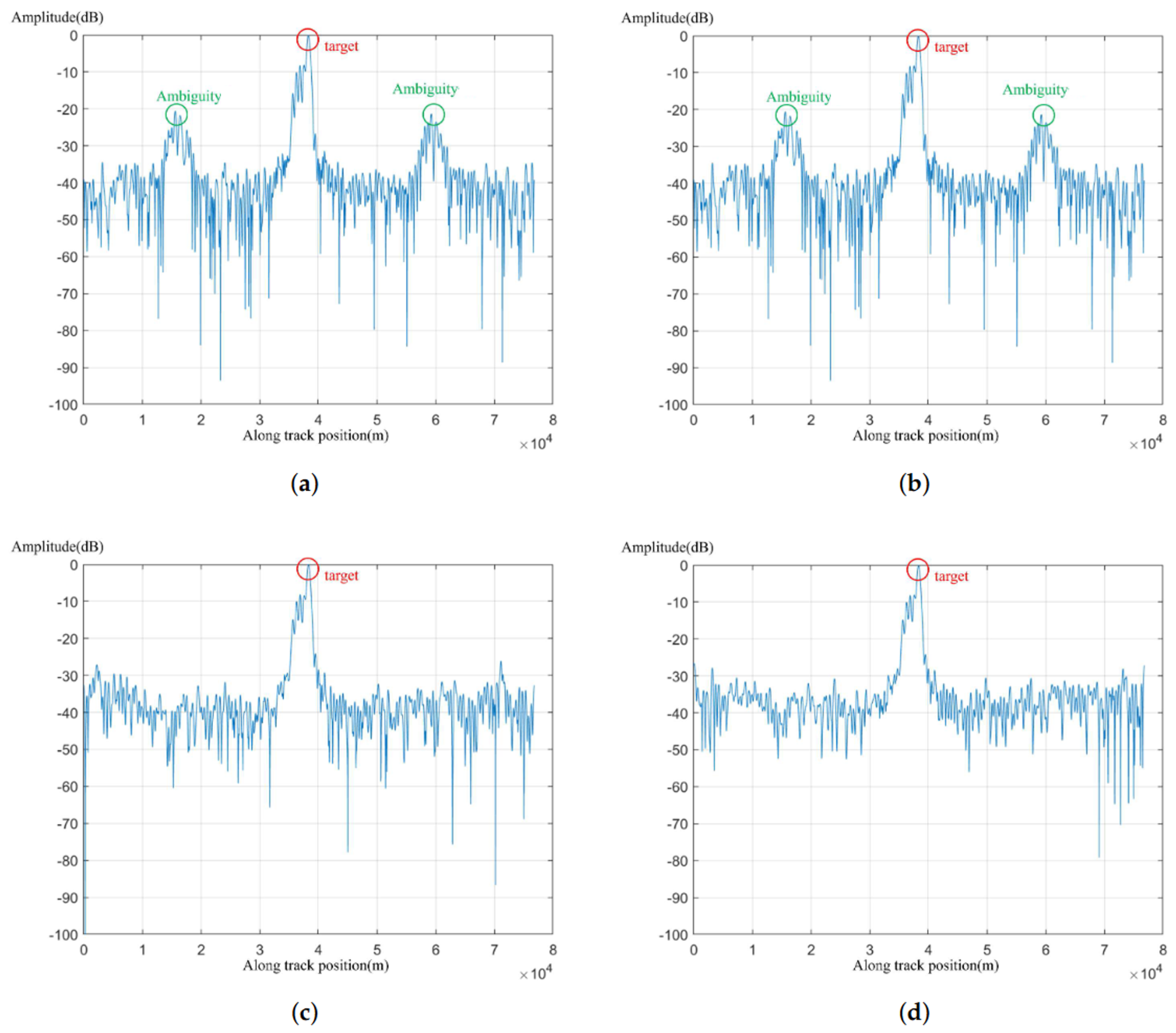
To better show the imaging effectiveness of the algorithms, we located the point of maximum value and conducted interpolation 16 times. The interpolated azimuthal slice is shown in Figure 9. This indicates that both the CS-IST-AAS algorithm and SAAS-Net can significantly reduce the side-lobes. In the results of CS-IST and ISTA-Net, there are two side peaks on the left and right sides of the main peak, which is known as azimuth ambiguity. This occurs due to an insufficient sampling rate in the azimuth direction, causing part of the main observation area’s spectrum to fold into the ambiguous region, thereby creating ambiguous energy. In the azimuth spectrum, this will appear as two symmetric peaks.

Figure 9.
Azimuth frequency spectrum of 4 algorithms with different SNRs: (a) without noise; (b) 20 dB noise; (c) 10 dB noise; (d) 5 dB noise.
The azimuthal results show that the algorithm proposed in this paper significantly reduces the azimuthal side-lobe, achieving the best suppression of azimuthal ambiguity rings. CS-IST-AAS also has some effect on ambiguity ring suppression. The CS-IST and ISTA-Net algorithms, on the other hand, do not perform additional sparse optimization of the azimuthal direction and thus suffer from spectral aliasing in the azimuthal direction when the azimuthal direction is undersampled. In the process of gradually reducing the sampling rate, the algorithm in this paper is relatively less affected, and the side flap suppression effect is relatively good. In the comparative experiment, 5 dB noise, 10 dB noise, 20 dB noise, and no noise were added, respectively. The results of the azimuthal frequency spectrum indicate that although the waveform underwent some changes after the addition of noise, the main viewing area and the ambiguity area could still be clearly distinguished, further confirming the robustness of the algorithm presented in this paper.
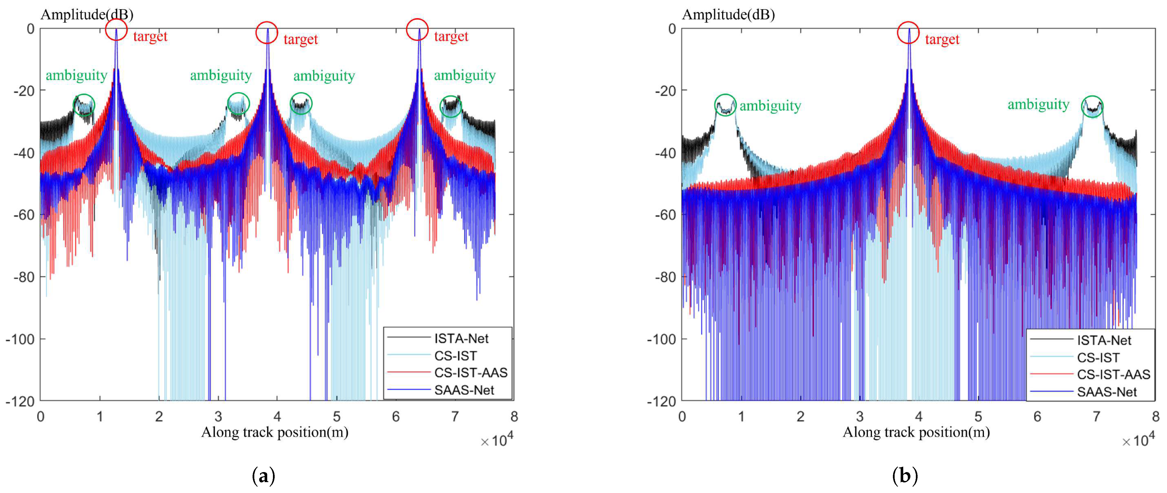
To further demonstrate the effectiveness of the method, imaging experiments with multiple point targets were designed. In Figure 10a, sparse imaging of three point targets uniformly distributed in the azimuth direction was performed, while in Figure 10b, sparse imaging of three point targets uniformly distributed in the range direction was carried out. It can be observed that, whether in the azimuth or range direction, SAAS-Net performs well in suppressing azimuthal ambiguity. Meanwhile, although the imaging effect of CS-IST-AAS is similar to that of SAAS-Net in single point target imaging experiments, in the imaging process of multiple point targets, SAAS-Net exhibits a significantly stronger suppression effect on side-lobes compared to CS-IST-AAS.
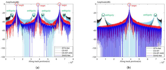
Figure 10.
Azimuth frequency spectrum of 4 algorithms with multiple targets: (a) targets in different azimuth directions; (b) targets in different range directions.
To show the effectiveness of the sampling pattern generated by our proposed network, we selected the same scene under 30% undersampling, 70% undersampling, and 90% undersampling and calculated the AASR at this point. The results of the experiments are shown in Table 3 in order to further demonstrate the superiority of this paper’s algorithm in azimuthal ambiguity suppression.
Table 3.
AASR under different undersampling patterns.
3.2. Real Data Experiments and Results
The data we used were sourced from the imaging results of the Gaofen-3 satellite on 30 March 2019, at 22:12:43. We used four algorithms, CS-IST, CS-IST-AAS, ISTA-Net, and SAAS-Net, to image the actual data. The imaging results are shown in Figure 11.
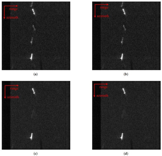
Figure 11.
Real data imaging results: (a) sparse imaging algorithm based on chirp-scaling; (b) unfolded network based on the chirp-scaling imaging algorithm; (c) traditional azimuth ambiguity suppression algorithm based on group sparsity; (d) SAAS-Net.
We selected an area with two ships for sparse SAR imaging. It can be observed that due to undersampling in the azimuth direction, both the conventional CS-IST algorithm and the ISTA-Net algorithm suffered from severe azimuth ambiguity, with artifacts appearing above or below the target ship. The presence of artifacts in the imaging scene is almost invisible in the imaging results using proposed method as well as the CS-IST-AAS algorithm. The imaging quality of the proposed algorithm and CS-IST-AAS was suppressed. In order to further compare the imaging results of these algorithms, the AASR and Frames Per Minute (FPM) of these four algorithms were compared. The results are shown in Table 4. It can be seen that the ambiguity suppression effect of proposed algorithm in the azimuthal direction was not significantly different from that of the CS-IST-AAS algorithm. At the same time, the imaging speed was much higher than that of the CS-IST-AAS algorithm.
Table 4.
Comparisons of AASR for ship target.
In order to compare the imaging quality of these algorithms, we calculated their AASR. At the same time, we also compared the imaging speed of these algorithms. The results are shown in Table 4. The algorithm in this paper had a comparable ambiguity suppression effect with the CS-IST-AAS algorithm, and the computational speed was improved by about 800 times compared to the CS-IST-AAS algorithm. Therefore, SAAS-Net can realize fast imaging with azimuthal ambiguity suppression.
We sliced the azimuthal direction of the real data. It can be seen in Figure 12 that the azimuthal side-lobes were significantly reduced in the algorithm of this paper and CS-IST-AAS, and the other two algorithms had significant ambiguity energy in the azimuthal direction.
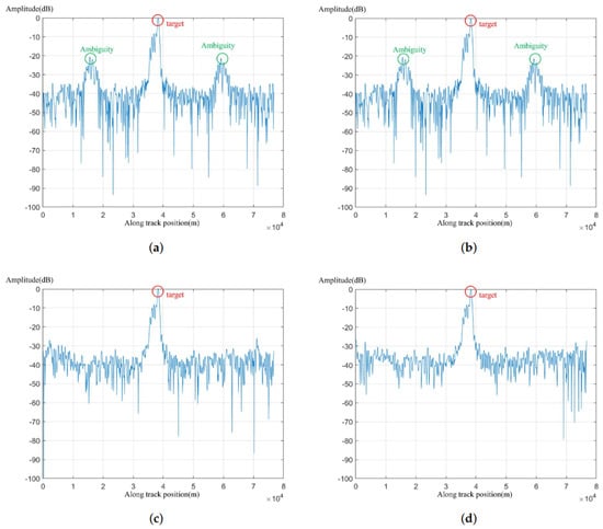
Figure 12.
Azimuth frequency spectrum: (a) CS-IST algorithm; (b) ISTA-Net; (c) CS-IST-AAS algorithm; (d) SAAS-Net.
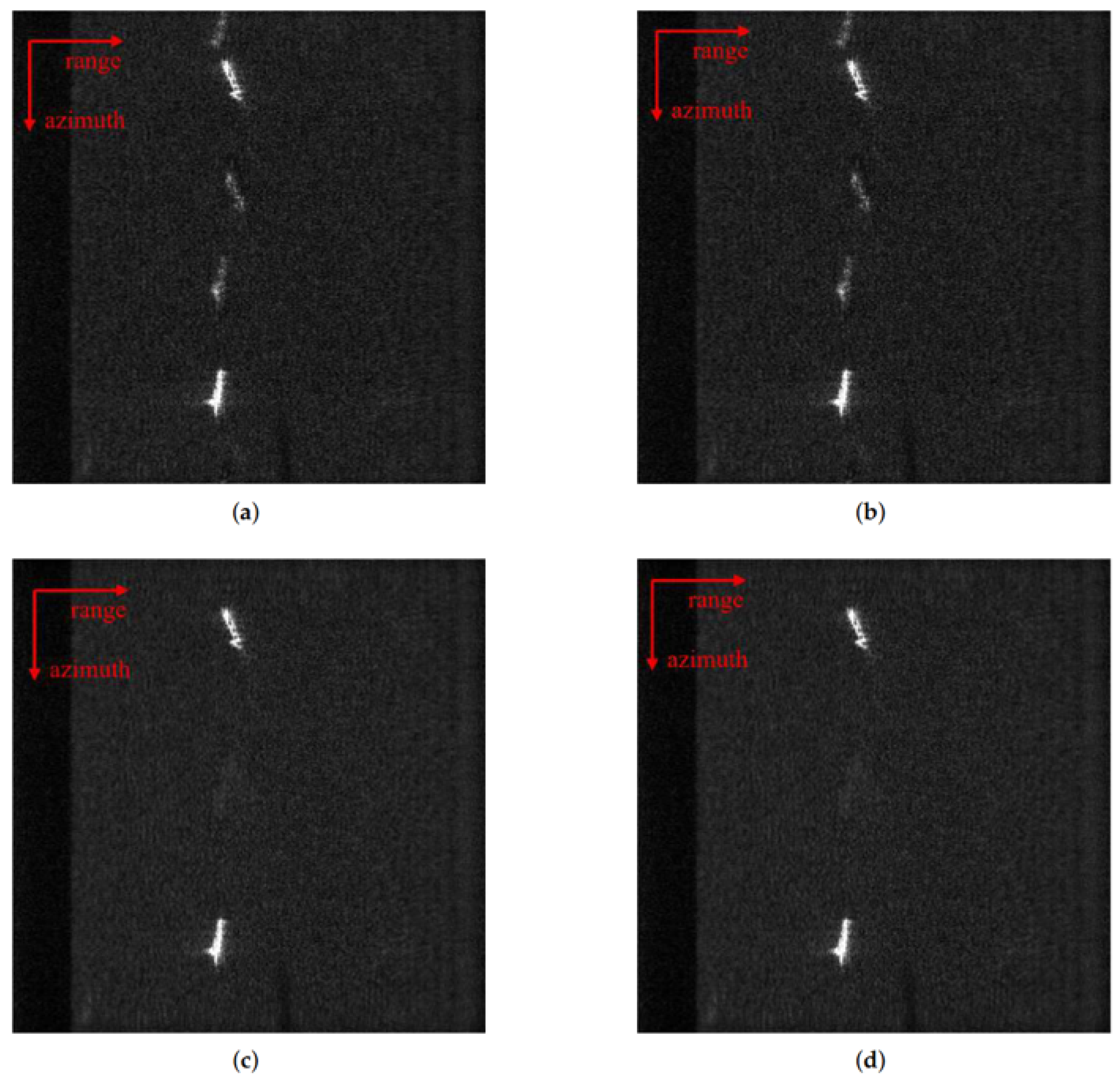
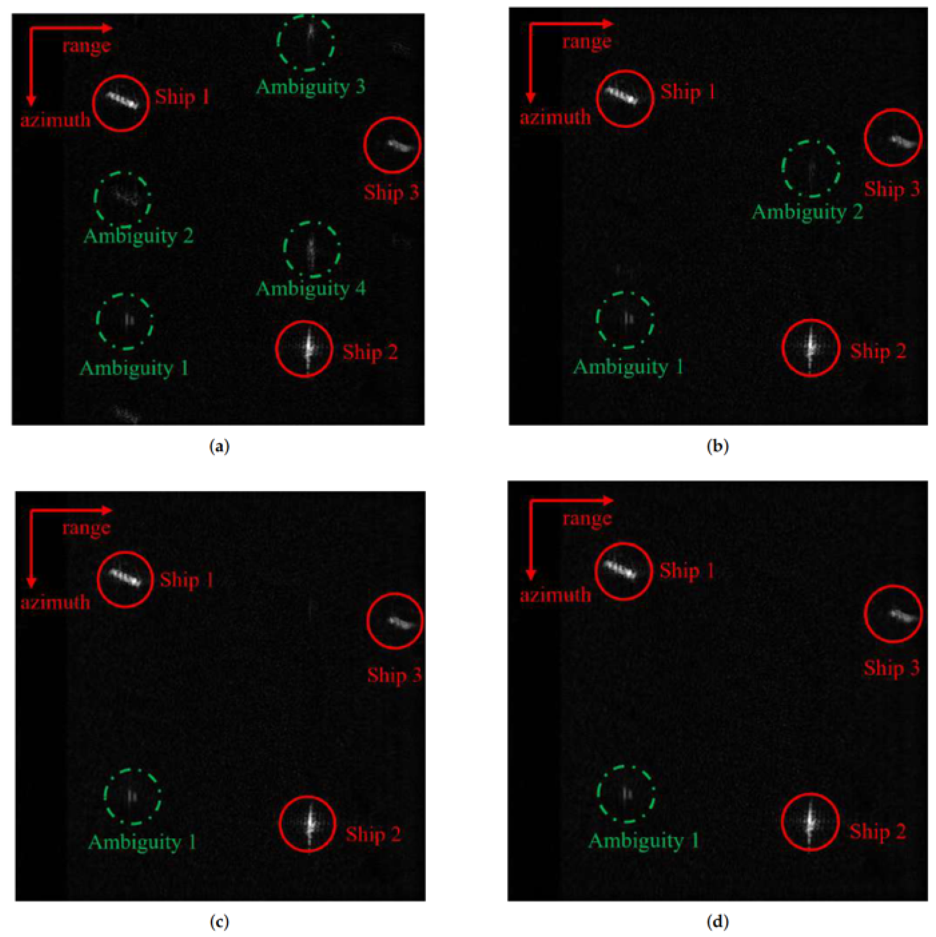
We conducted comparative experiments using ISTA-net and the proposed network at undersampling rates of 80%, 60%, and 30%, adding 20 dB of noise throughout the experiment. The results are presented in Figure 13. We chose a region with a single ship to perform sparse SAR imaging.

Figure 13.
Imaging results after azimuth undersampling: (a) result of ISTA-Net with 80% azimuth undersampling; (b) result of AAS-Net with 80% azimuth undersampling; (c) result of ISTA-Net with 60% azimuth undersampling; (d) result of AAS-Net with 60% azimuth undersampling; (e) result of ISTA-Net with 30% azimuth undersampling; (f) result of AAS-Net with 30% azimuth undersampling.
There are three ships that can be seen in Figure 13a. In fact, the center portion represents the actual ship that was imaged, while the ships above and below are artifacts were due to azimuthal ambiguity. At a undersampling rate of 80%, artifacts in the upper and lower vessels due to orientation ambiguity were visible with ISTA-net, while these ambiguity artifacts were barely noticeable in the proposed network. At a undersampling rate of 60%, the artifacts in ISTA-net became more prominent, and a slight artifact also appeared in the proposed network. At a undersampling rate of 30%, both algorithms exhibited clear artifacts, but the ambiguity energy in the proposed network remained significantly lower than that in ISTA-net, demonstrating the effectiveness of the proposed algorithm in suppressing ambiguity energy in the azimuth direction. This demonstrates that the algorithm presented in this paper effectively suppresses ambiguity energy in the azimuth direction. At the same time, the algorithm in this paper is robust to noise.
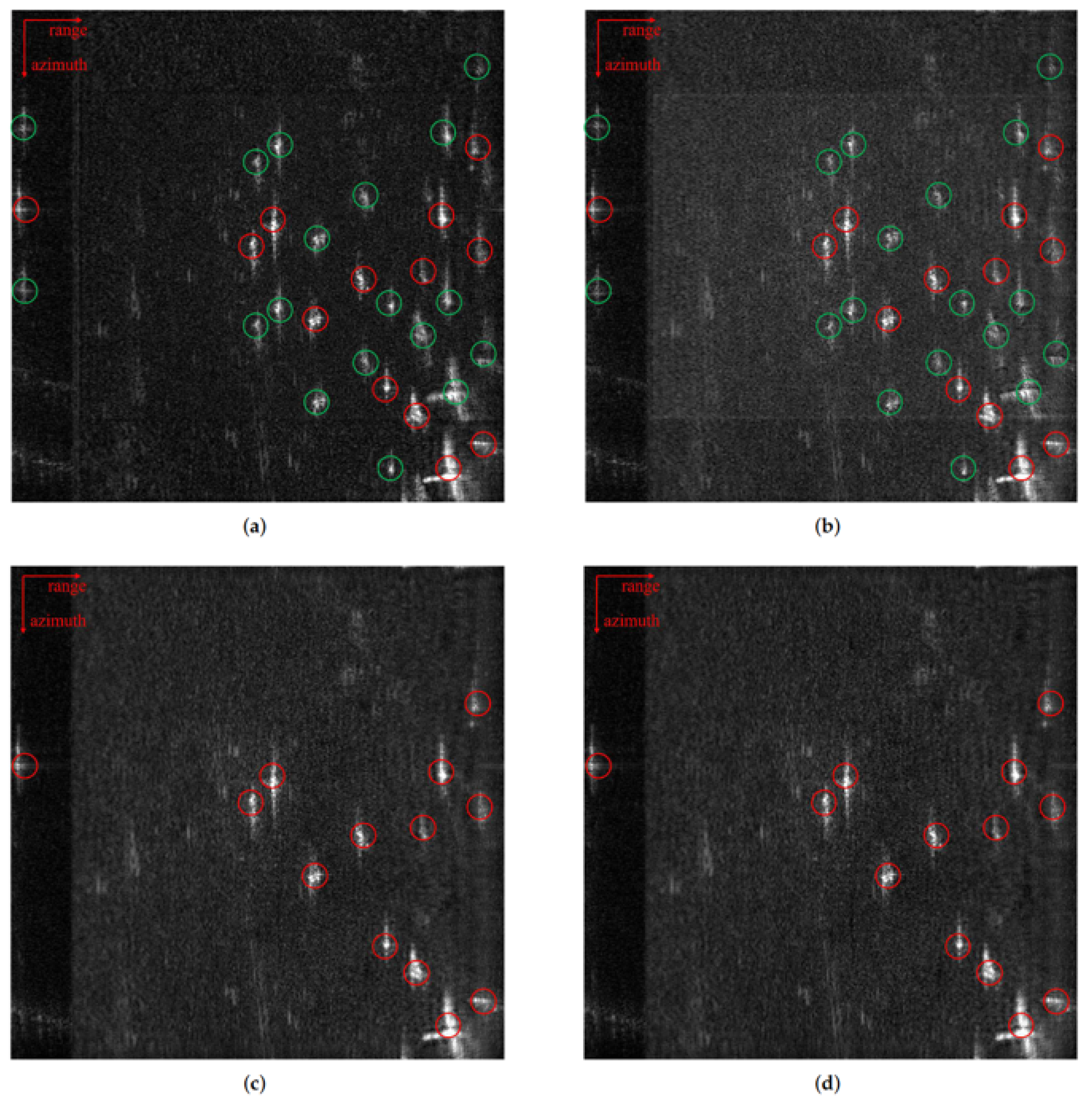
To further investigate the imaging performance of the algorithm in complex scenes, an imaging experiment was conducted with a scene containing 13 ships. In this complex scene, some targets are closely connected, and the real targets of some objects are close to the ghost images of other real targets. The imaging results are shown in Figure 14. It can be observed that both the SAAS-Net and CS-IST-AAS algorithms effectively suppress azimuthal ambiguity, while the imaging results of the ISTA-Net and CS-IST algorithms show obvious ghost images. This further confirms the effectiveness of the algorithm presented in this paper.
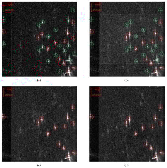
Figure 14.
Multiple scattered target imaging results: (a) CS-IST; (b) ISTA-Net; (c) CS-IST-AAS; (d) SAAS-Net.
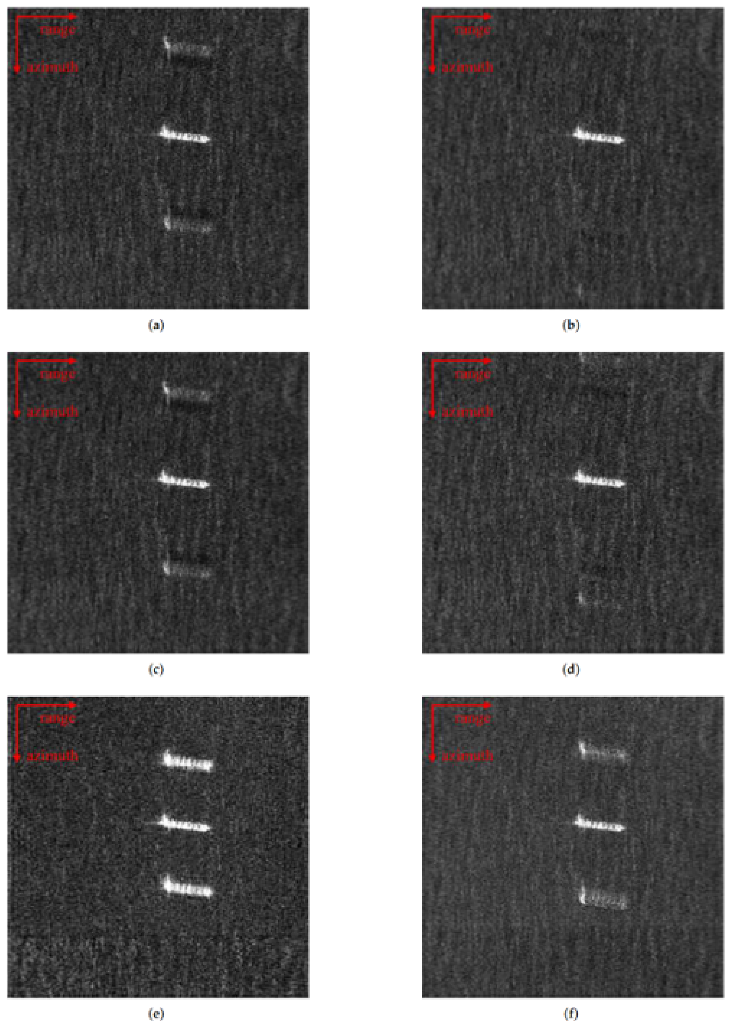
In order to further demonstrate the structural properties of the SAAS-Net, we show the imaging outputs for each layer of the imaging process in Figure 15. There are three ships in the imaging area. It can be seen that when there is one iterative layer, the outline of the imaging gradually appears, but it still has significant azimuth ambiguity. With the increase in the number of iterative layers, the imaging quality gradually improves. It reaches the highest quality when there are five iterative layers, after which the change is no longer obvious.
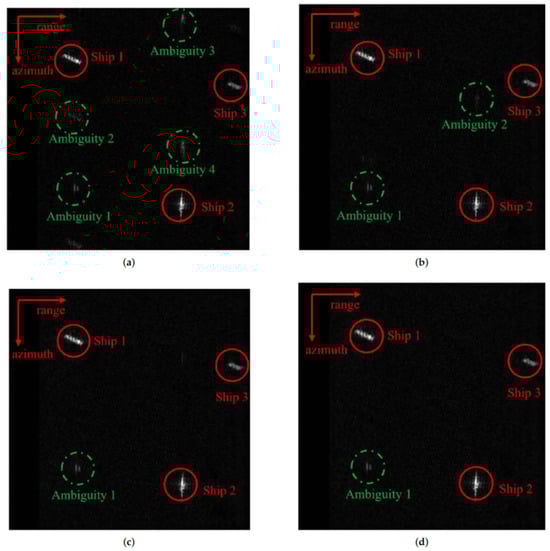
Figure 15.
Imaging results with different iteration layers: (a) one layer; (b) three layers; (c) five layers; (d) seven layers.
As a result, the network essentially reaches convergence by the fifth layer, and with the overall network structure being relatively shallow, the training process can be completed quickly, thereby further enhancing imaging efficiency. Meanwhile, 20 dB of Gaussian noise was added in this experiment, and the imaging results were still clear. This also proves the robustness of the proposed algorithm.
4. Discussion
We proposed the Self-supervised Azimuth Ambiguity Suppression Network (SAAS-Net), a novel algorithm designed to effectively suppression azimuth ambiguity in sparse SAR imaging. Through comprehensive simulation and real data experiments, we demonstrated the superior performance of SAAS-Net in terms of both azimuth ambiguity suppression and computational efficiency.
The experimental results clearly indicate that SAAS-Net can significantly reduce azimuth ambiguity, outperforming traditional algorithms in terms of both suppression effectiveness and processing speed. While conventional methods rely heavily on intricate computations, SAAS-Net leverages group sparsity to effectively address azimuth ambiguity, leading to a more efficient and accurate solution. Additionally, in the scenario with multiple point targets, the imaging performance of SAAS-Net was slightly better than that of the CS-IST-AAS algorithm. The algorithm’s ability to maintain high performance while achieving faster processing times highlights its practical potential for real-time SAR imaging applications.
We also conducted experiments under undersampling conditions to investigate the algorithm’s robustness when the azimuth sampling rate was insufficient. As expected, azimuth ambiguity was still observed under low sampling rates. However, the results clearly showed that SAAS Net significantly mitigated the impact of this ambiguity compared to traditional methods. While some residual ambiguity remained, the suppression capabilities of SAAS Net were evident, suggesting its robustness even in challenging conditions of insufficient sampling.
5. Conclusions
Azimuth ambiguity remains a significant challenge in SAR imaging, severely affecting image quality and hindering the performance of conventional SAR applications. Limited by the azimuth sampling rate, azimuth ambiguity becomes particularly problematic in sparse SAR imaging scenarios. To address this issue, this article proposed SAAS-Net, a novel sparse SAR imaging unfolded network designed to suppress azimuth ambiguity efficiently. We introduced a unique encoder–decoder network structure within SAAS-Net, where the encoder generates reference imaging results and facilitates a self-supervised training process, while the decoder is responsible for the actual imaging procedure. This architecture enables SAAS-Net to learn from data directly, optimizing the parameters through end-to-end training. As a result, the network adapts automatically without requiring complex manual tuning, making the process both efficient and user-friendly. The core advantage of SAAS-Net lies in its ability to suppress azimuth ambiguity, even under undersampling conditions, thus preserving the inherent benefits of sparse SAR imaging. This solution not only enhances the quality of the resulting images but also accelerates the entire imaging process, reducing computational costs without sacrificing accuracy. To validate the effectiveness of SAAS-Net, we conducted imaging experiments on both simulated and real datasets. The results clearly demonstrate the efficiency of our proposed algorithm in suppressing azimuth ambiguity, achieving better performance than traditional methods. Moreover, the algorithm’s ability to handle undersampled data and still produce high-quality imaging results underscores its robustness in SAR applications, where undersampling and noisy conditions are often encountered.
In summary, the proposed SAAS-Net algorithm presents a preliminary exploration into addressing azimuth ambiguity in sparse SAR imaging. Preliminary experimental results indicate that the method exhibits certain robustness under undersampled conditions and noise interference, offering a new technical approach to improving sparse SAR imaging quality. However, the algorithm’s generalizability to highly complex real-world scenarios—such as extreme undersampling or dynamic target environments—still requires further validation. Future work will focus on refining the network architecture, exploring its adaptability across broader operational scenarios.
Author Contributions
Z.J.: Conceptualization; methodology; validation; writing—original draft; writing—review and editing. Z.P.: Conceptualization; supervision; writing—review and editing. Z.Z.: Funding; conceptualization; supervision; writing—review and editing. X.Q.: Conceptualization; resources; supervision; writing—review and editing. All authors have read and agreed to the published version of the manuscript.
Funding
This work is supported by National Key R&D Program of China under grant #2023YFB3904900.
Data Availability Statement
The datasets presented in this article are not readily available because the data are part of an ongoing study. Requests to access the datasets should be directed to jinzhiyi17@mails.ucas.ac.cn.
Conflicts of Interest
The authors declare no conflicts of interest.
Abbreviations
The following abbreviations are used in this manuscript:
| HRWS | High-Resolution Wide-Swath |
| SAR | Synthetic Aperture Radar |
| RCM | Range Cell Migration |
| CS-IST | Chirp Scaling-Iterative Shrinkage Thresholding |
| AAS-Net | Azimuth Ambiguity Suppression Network |
| CS | Chirp-Scaling |
| PRF | Pulse Repetition Frequency |
| ISTA | Iterative Shrinkage Thresholding Algorithm |
| FISTA | Fast Iterative Shrinkage Thresholding Algorithm |
| PSLR | Peak Side-Lobe Ratio |
| ISLR | Integral Side-Lobe Ratio |
| AASR | Azimuth Ambiguity Signal Ratio |
| FPM | Frames Per Minute |
References
- Nyquist, H. Thermal agitation of electric charge in conductors. Phys. Rev. 1928, 32, 110. [Google Scholar]
- Baraniuk, R.G. Compressive sensing [lecture notes]. IEEE Signal Process. Mag. 2007, 24, 118–121. [Google Scholar]
- Candès, E.J.; Romberg, J.; Tao, T. Robust uncertainty principles: Exact signal reconstruction from highly incomplete frequency information. IEEE Trans. Inf. Theory 2006, 52, 489–509. [Google Scholar]
- Patel, V.M.; Easley, G.R.; Healy, D.M.; Chellappa, R. Compressed synthetic aperture radar. IEEE J. Sel. Top. Signal Process. 2010, 4, 244–254. [Google Scholar]
- Dong, X.; Zhang, Y. SAR image reconstruction from undersampled raw data using maximum a posteriori estimation. IEEE J. Sel. Top. Appl. Earth Obs. Remote Sens. 2014, 8, 1651–1664. [Google Scholar]
- Yang, D.; Liao, G.; Zhu, S.; Yang, X.; Zhang, X. SAR imaging with undersampled data via matrix completion. IEEE Geosci. Remote Sens. Lett. 2014, 11, 1539–1543. [Google Scholar]
- Zeng, J.; Fang, J.; Xu, Z. Sparse SAR imaging based on L 1/2 regularization. Sci. China Inf. Sci. 2012, 55, 1755–1775. [Google Scholar]
- Du, X.; Duan, C.; Hu, W. Sparse representation based autofocusing technique for ISAR images. IEEE Trans. Geosci. Remote Sens. 2012, 51, 1826–1835. [Google Scholar]
- Zhang, L.; Xing, M.; Qiu, C.W.; Li, J.; Bao, Z. Achieving higher resolution ISAR imaging with limited pulses via compressed sampling. IEEE Geosci. Remote Sens. Lett. 2009, 6, 567–571. [Google Scholar]
- Aguilera, E.; Nannini, M.; Reigber, A. A data-adaptive compressed sensing approach to polarimetric SAR tomography of forested areas. IEEE Geosci. Remote Sens. Lett. 2012, 10, 543–547. [Google Scholar]
- Austin, C.D.; Ertin, E.; Moses, R.L. Sparse signal methods for 3-D radar imaging. IEEE J. Sel. Top. Signal Process. 2010, 5, 408–423. [Google Scholar]
- Budillon, A.; Ferraioli, G.; Schirinzi, G. Localization performance of multiple scatterers in compressive sampling SAR tomography: Results on COSMO-SkyMed data. IEEE J. Sel. Top. Appl. Earth Obs. Remote Sens. 2014, 7, 2902–2910. [Google Scholar]
- Fang, J.; Xu, Z.; Zhang, B.; Hong, W.; Wu, Y. Fast compressed sensing SAR imaging based on approximated observation. IEEE J. Sel. Top. Appl. Earth Obs. Remote Sens. 2013, 7, 352–363. [Google Scholar]
- Wu, Y.; Zhang, Z.; Qiu, X.; Zhao, Y.; Yu, W. MF-JMoDL-Net: A Sparse SAR Imaging Network for Undersampling Pattern Design towards Suppressed Azimuth Ambiguity. IEEE Trans. Geosci. Remote Sens. 2024, 62, 5212018. [Google Scholar]
- Mason, E.; Yonel, B.; Yazici, B. Deep learning for SAR image formation. In Proceedings of the Algorithms for Synthetic Aperture Radar Imagery XXIV; SPIE: Bellingham, WA, USA, 2017; Volume 10201, pp. 11–21. [Google Scholar]
- Pu, W. Deep SAR imaging and motion compensation. IEEE Trans. Image Process. 2021, 30, 2232–2247. [Google Scholar]
- Zhao, S.; Ni, J.; Liang, J.; Xiong, S.; Luo, Y. End-to-end SAR deep learning imaging method based on sparse optimization. Remote Sens. 2021, 13, 4429. [Google Scholar] [CrossRef]
- Li, M.; Wu, J.; Huo, W.; Jiang, R.; Li, Z.; Yang, J.; Li, H. Target-oriented SAR imaging for SCR improvement via deep MF-ADMM-Net. IEEE Trans. Geosci. Remote Sens. 2022, 60, 1–14. [Google Scholar]
- Gregor, K.; LeCun, Y. Learning fast approximations of sparse coding. In Proceedings of the 27th International Conference on on Machine Learning, Haifa, Israel, 21–24 June 2010; pp. 399–406. [Google Scholar]
- Wang, M.; Wei, S.; Liang, J.; Zeng, X.; Wang, C.; Shi, J.; Zhang, X. RMIST-Net: Joint range migration and sparse reconstruction network for 3-D mmW imaging. IEEE Trans. Geosci. Remote Sens. 2021, 60, 1–17. [Google Scholar]
- Yonel, B.; Mason, E.; Yazıcı, B. Deep learning for passive synthetic aperture radar. IEEE J. Sel. Top. Signal Process. 2017, 12, 90–103. [Google Scholar] [CrossRef]
- Di Martino, G.; Iodice, A.; Riccio, D.; Ruello, G. Filtering of azimuth ambiguity in stripmap synthetic aperture radar images. IEEE J. Sel. Top. Appl. Earth Obs. Remote Sens. 2014, 7, 3967–3978. [Google Scholar] [CrossRef]
- Moreira, A. Suppressing the azimuth ambiguities in synthetic aperture radar images. IEEE Trans. Geosci. Remote Sens. 1993, 31, 885–895. [Google Scholar] [CrossRef]
- Zhang, B.; Jiang, C.; Zhang, Z.; Fang, J.; Zhao, Y.; Wen, H.; Wu, Y.; Xu, Z. Azimuth Ambiguity Suppression for SAR Imaging based on Group Sparse Reconstruction. In Proceedings of the 2nd International Workshop on Compressed Sensing Applied to Radar, Bonn, Germany, 17–19 September 2013; pp. 17–19. [Google Scholar]
- Xu, G.; Xia, X.G.; Hong, W. Nonambiguous SAR image formation of maritime targets using weighted sparse approach. IEEE Trans. Geosci. Remote Sens. 2017, 56, 1454–1465. [Google Scholar]
- Peng, X.; Youming, W.; Ze, Y. A SAR image azimuth ambiguity suppression method based on compressed sensing restoration algorithm. J. Radar 2016, 5, 39–45. [Google Scholar]
- Wu, Y.; Yu, Z.; Xiao, P.; Li, C. Azimuth ambiguity suppression based on minimum mean square error estimation. In Proceedings of the 2015 IEEE International Geoscience and Remote Sensing Symposium (IGARSS), Milan, Italy, 13–18 July 2015; pp. 2425–2428. [Google Scholar]
- Wu, Y.; Yu, Z.; Xiao, P.; Li, C. Suppression of azimuth ambiguities in spaceborne SAR images using spectral selection and extrapolation. IEEE Trans. Geosci. Remote Sens. 2018, 56, 6134–6147. [Google Scholar]
- Jingqiu, H.; Falin, L.; Chongbin, Z.; Bo, L.; Dongjin, W. CS-SAR imaging method based on inverse omega-K algorithm. J. Radars 2017, 6, 25–33. [Google Scholar]
- Barlow, J.F.R. The Chirp Scaling Algorithm for Synthetic Aperture Radar. Proc. IEEE 1979, 67, 789–791. [Google Scholar]

Disclaimer/Publisher’s Note: The statements, opinions and data contained in all publications are solely those of the individual author(s) and contributor(s) and not of MDPI and/or the editor(s). MDPI and/or the editor(s) disclaim responsibility for any injury to people or property resulting from any ideas, methods, instructions or products referred to in the content. |
© 2025 by the authors. Licensee MDPI, Basel, Switzerland. This article is an open access article distributed under the terms and conditions of the Creative Commons Attribution (CC BY) license (https://creativecommons.org/licenses/by/4.0/).