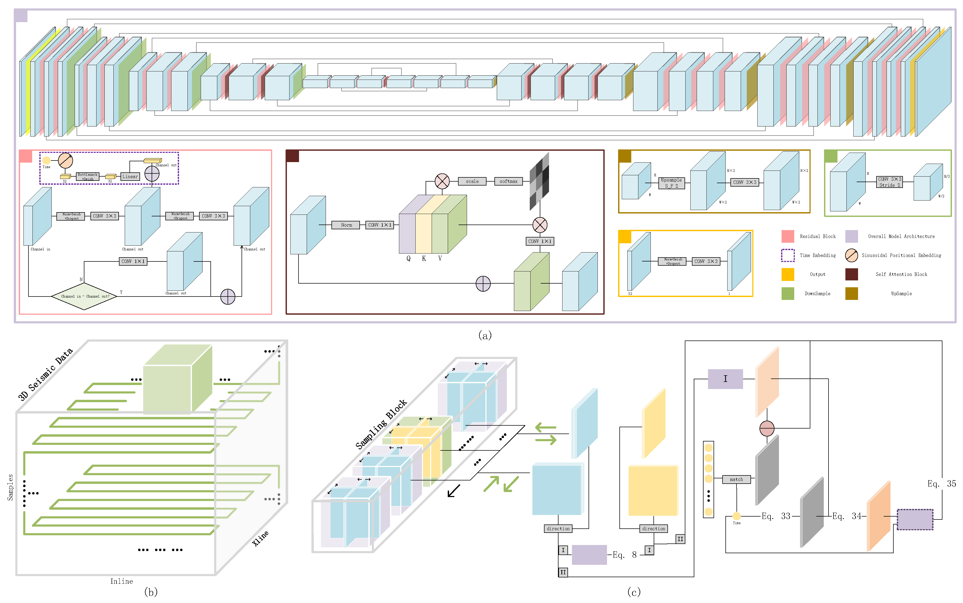
Figure 1.
Architecture of SSDn-DDPM. (a) The network architectures used in the noise estimation model and the diffusion model. (b) Illustration of the 3D serpentine sampling. (c) Illustration of the diffusion model training process.
Figure 1.
Architecture of SSDn-DDPM. (a) The network architectures used in the noise estimation model and the diffusion model. (b) Illustration of the 3D serpentine sampling. (c) Illustration of the diffusion model training process.
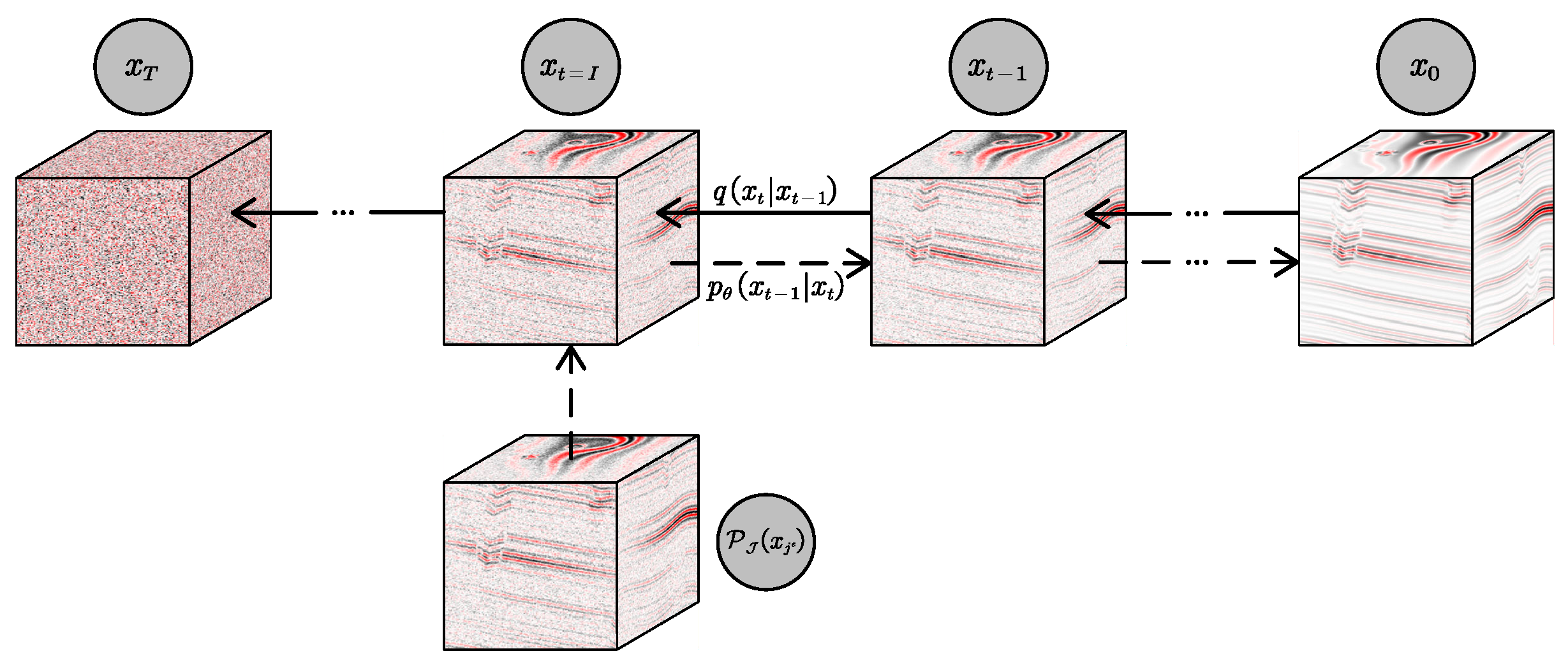
Figure 2.
Illustration of the forward and reverse processes of SSDn-DDPM.
Figure 2.
Illustration of the forward and reverse processes of SSDn-DDPM.
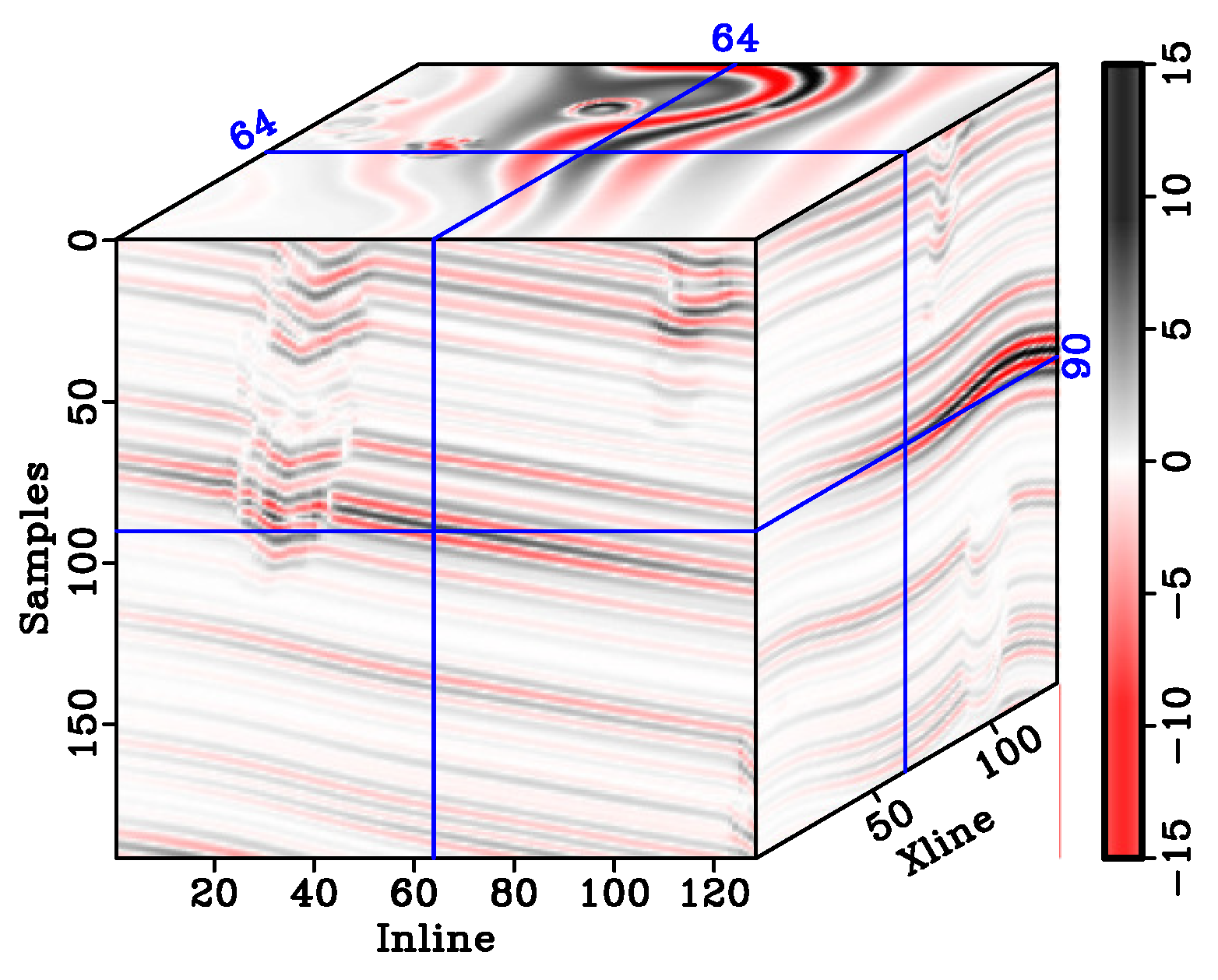
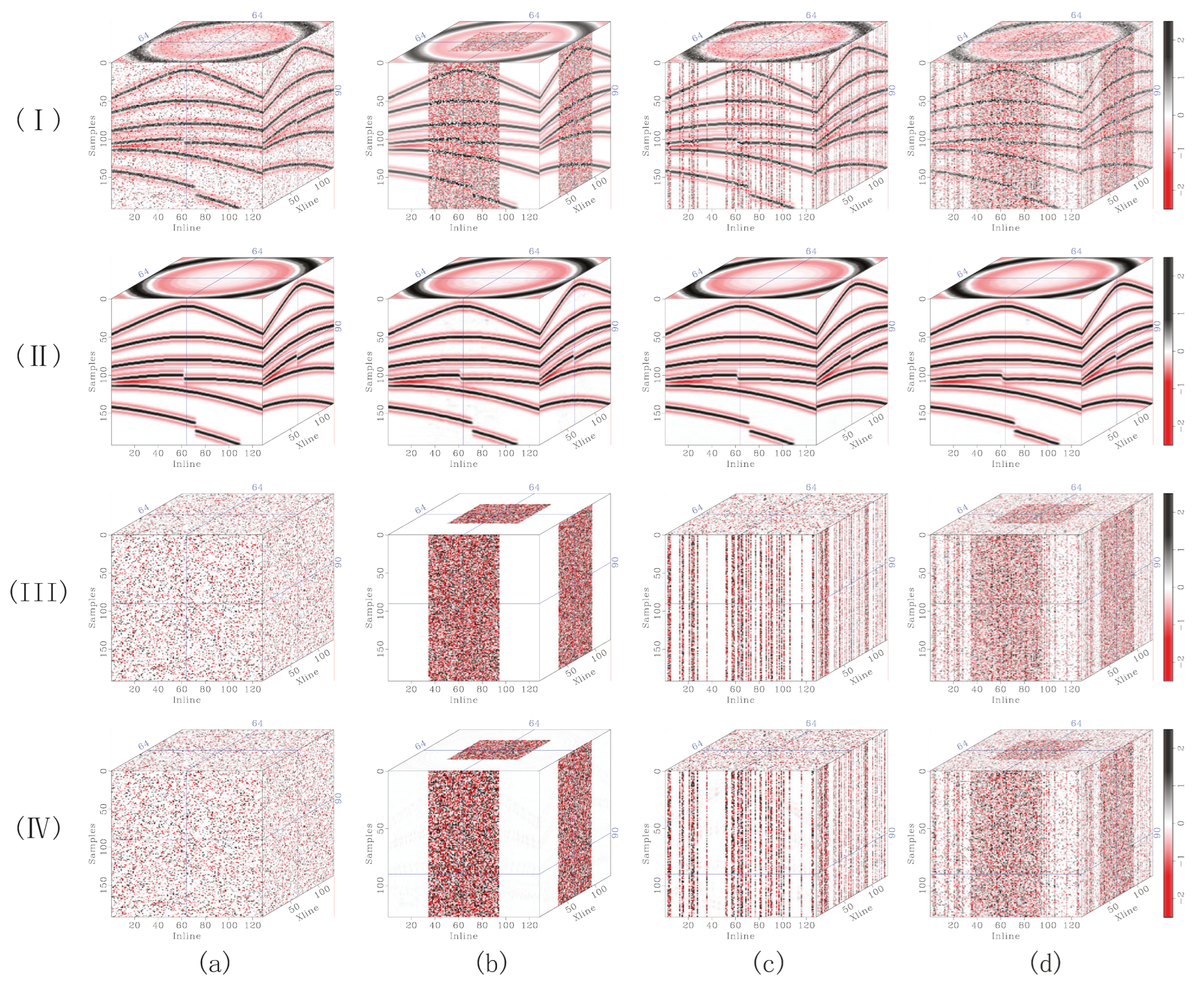
Figure 3.
Noiseless original synthetic seismic record.
Figure 3.
Noiseless original synthetic seismic record.
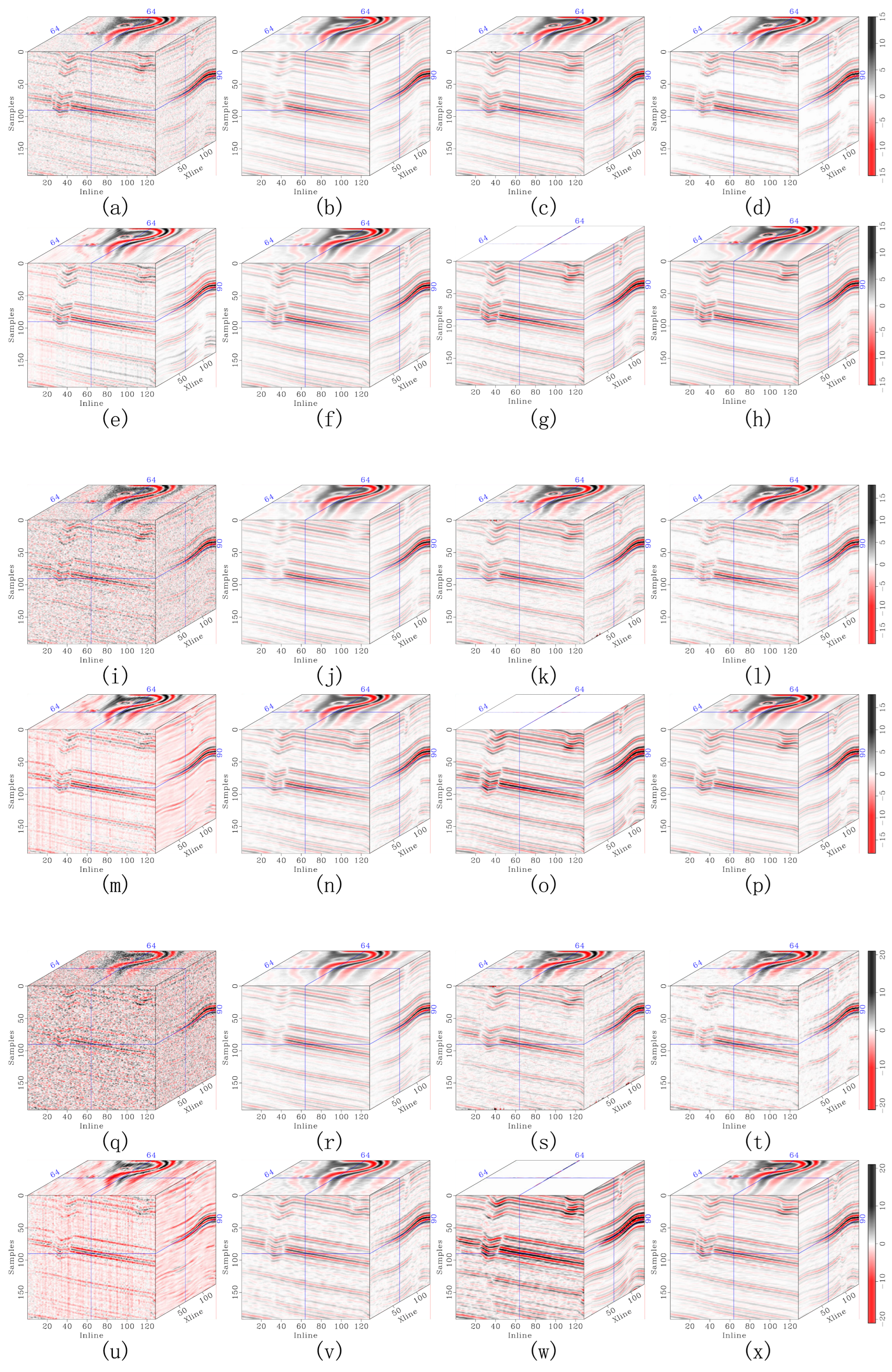
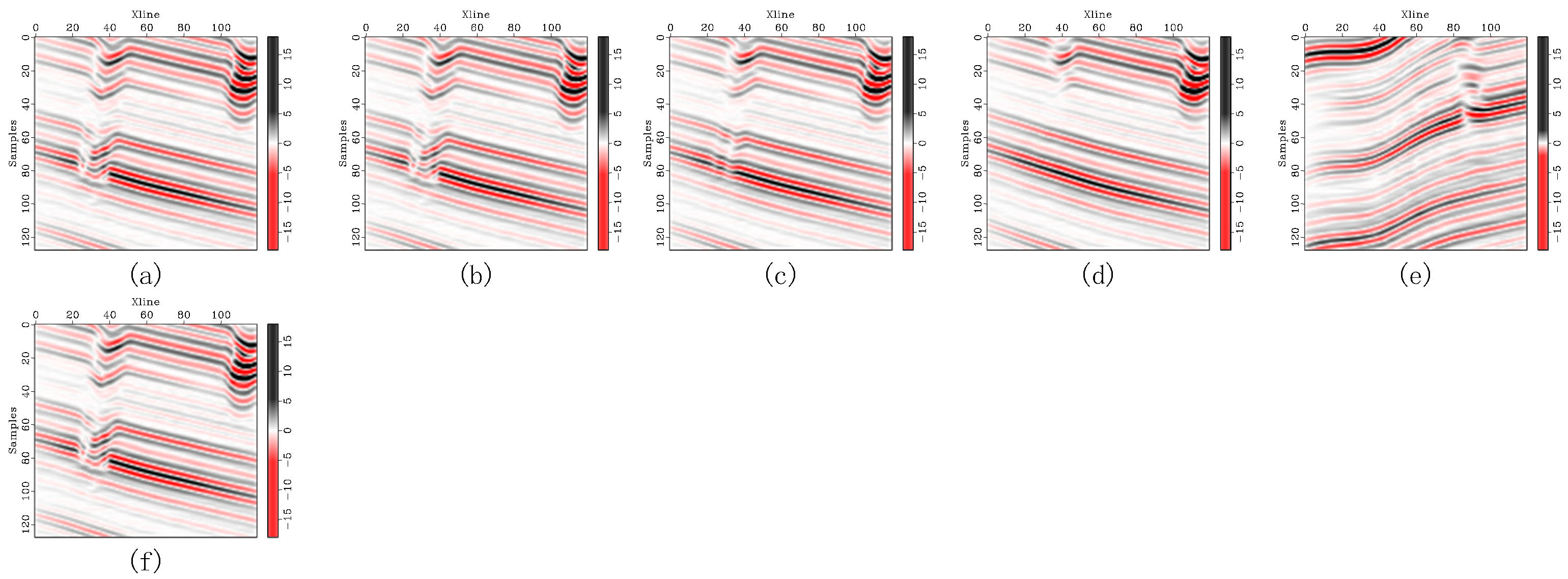
Figure 4.
Denoising comparison for synthetic seismic records: (a–h) show denoising results under light noise contamination, (i–p) under moderate noise contamination, and (q–x) under heavy noise contamination. For each noise level, (a–x) sequentially present the noisy data followed by the denoised results corresponding to DRR, SOSVMF, SGK, SeisGAN, DIP, PCADDPM, and SSDn-DDPM.
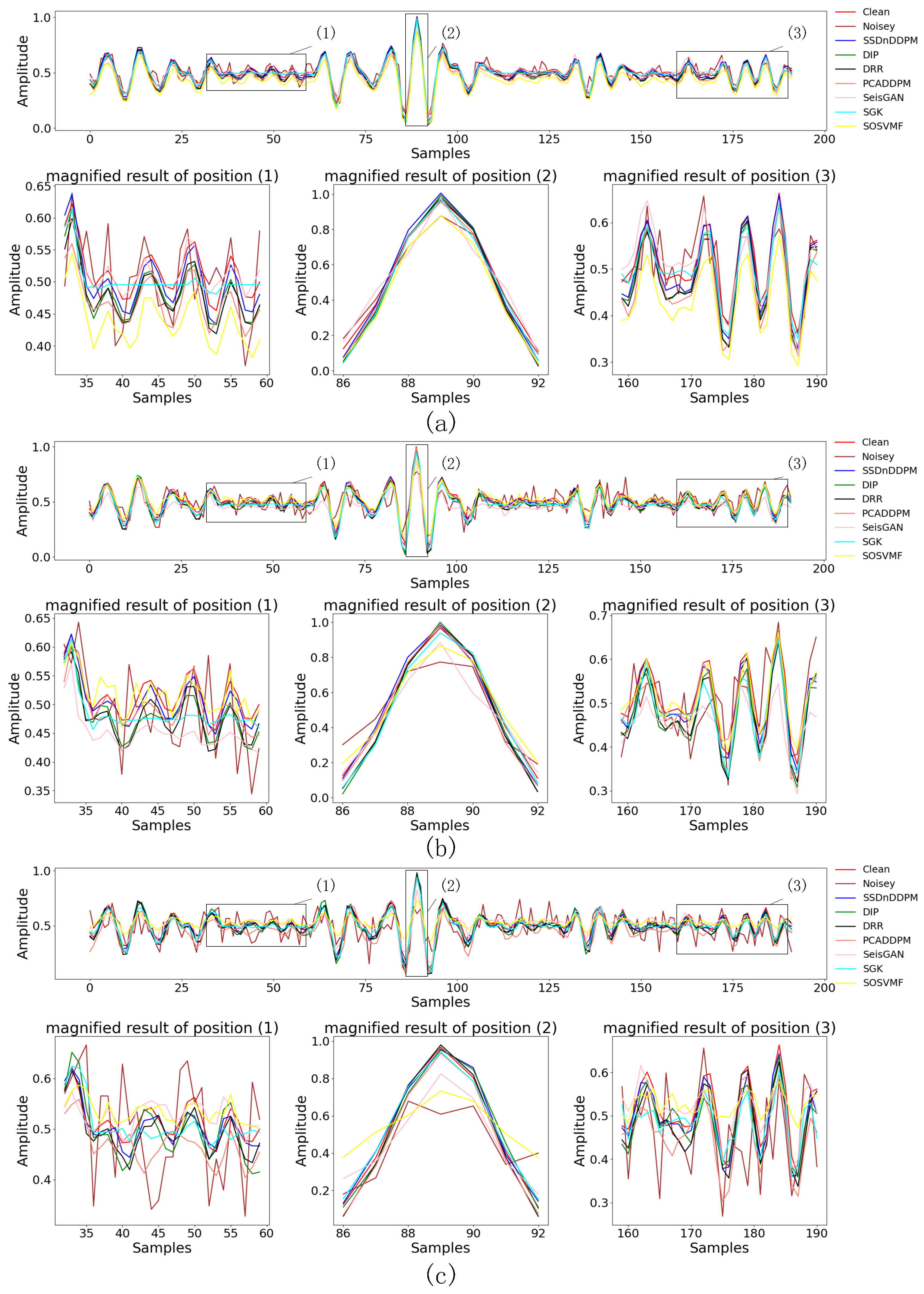
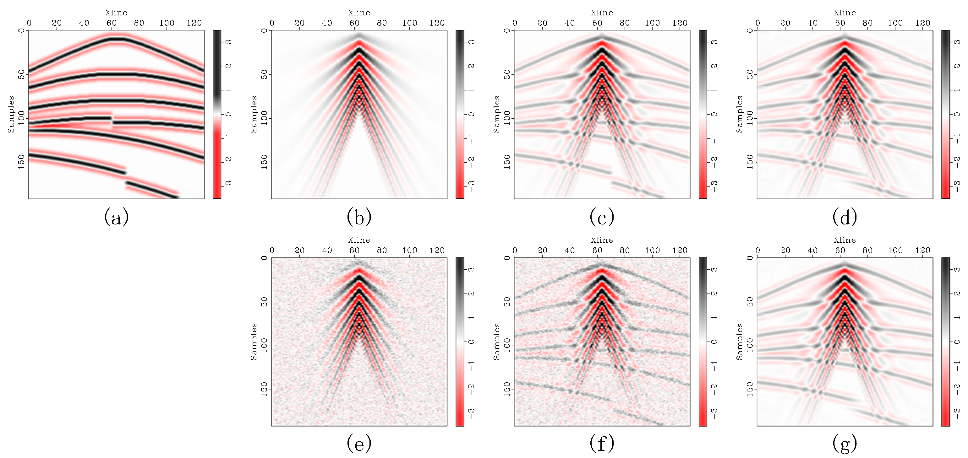
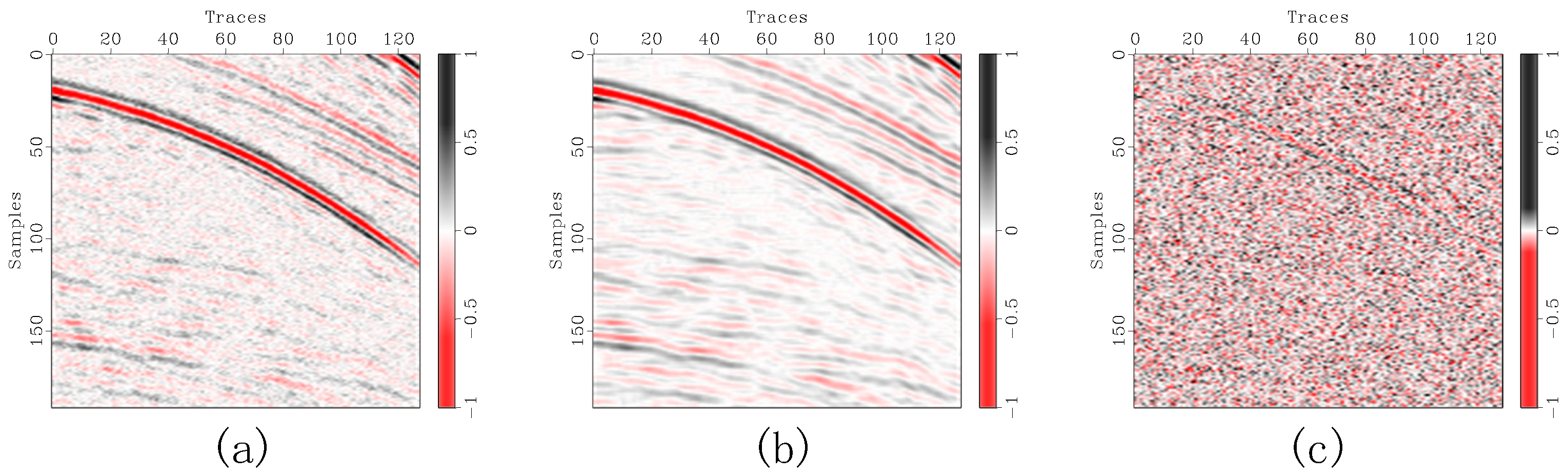
Figure 5.
Seismic single-trace comparison for synthetic records with (a) light, (b) moderate, and (c) heavy noise contamination.
Figure 5.
Seismic single-trace comparison for synthetic records with (a) light, (b) moderate, and (c) heavy noise contamination.
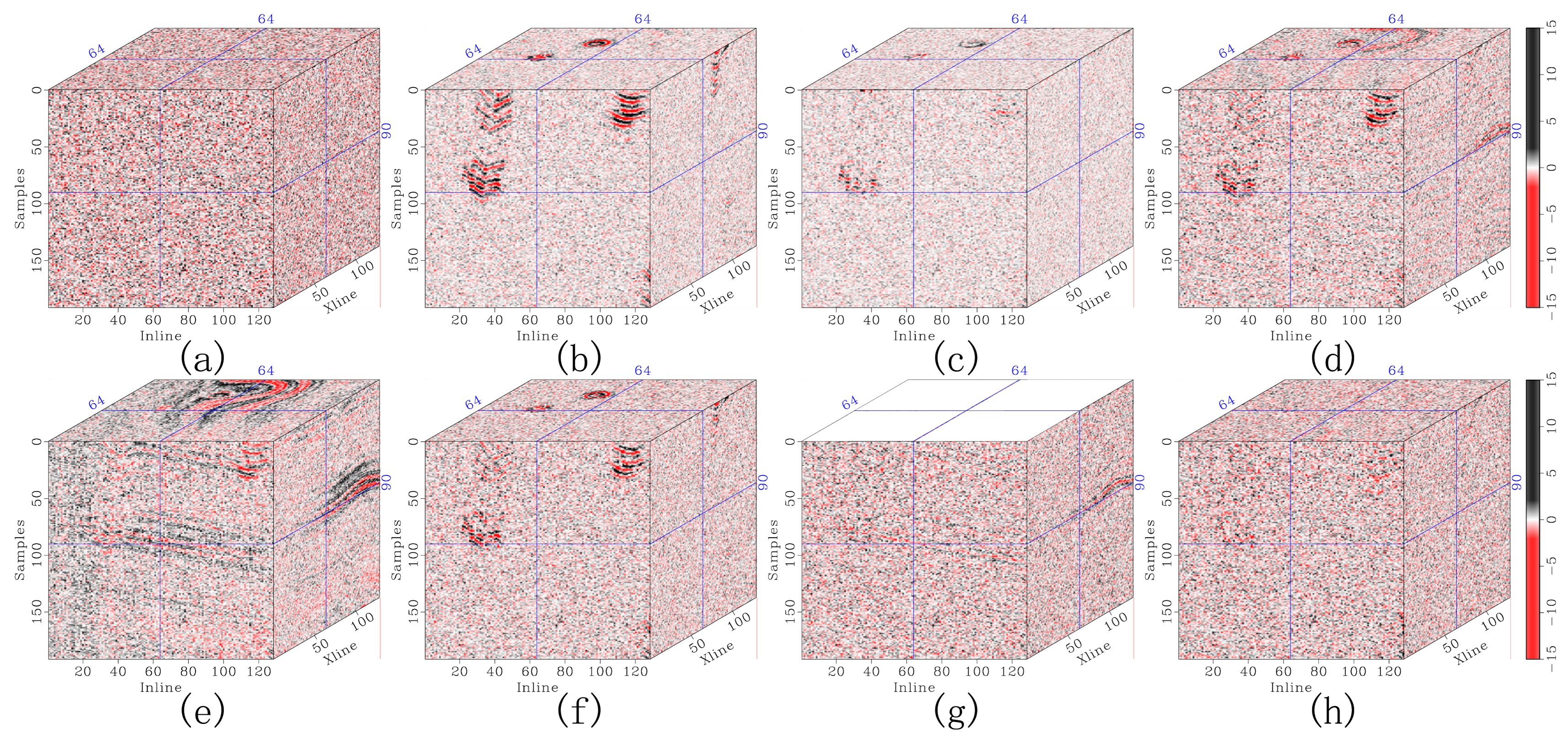
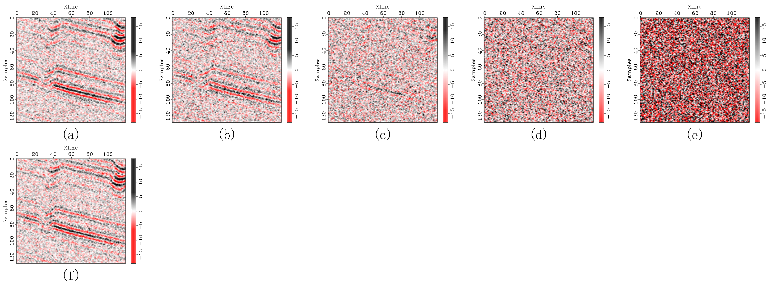
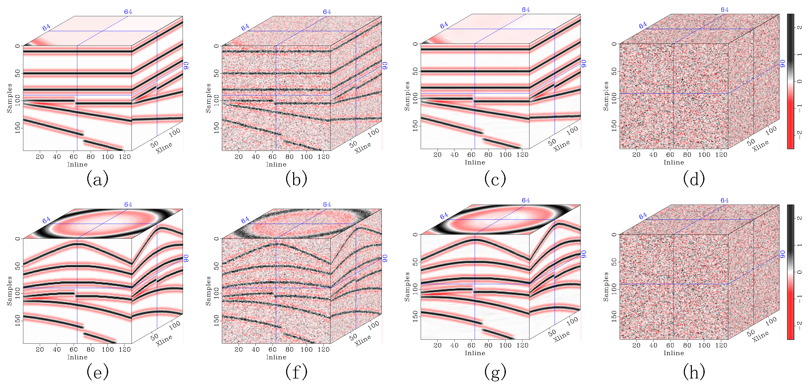
Figure 6.
Comparison of removed noise in synthetic seismic records with light noise contamination. The removed noise corresponds to (a) the original record, (b) DRR, (c) SOSVMF, (d) SGK, (e) SeisGAN, (f) DIP, (g) PCADDPM, and (h) SSDn-DDPM.
Figure 6.
Comparison of removed noise in synthetic seismic records with light noise contamination. The removed noise corresponds to (a) the original record, (b) DRR, (c) SOSVMF, (d) SGK, (e) SeisGAN, (f) DIP, (g) PCADDPM, and (h) SSDn-DDPM.
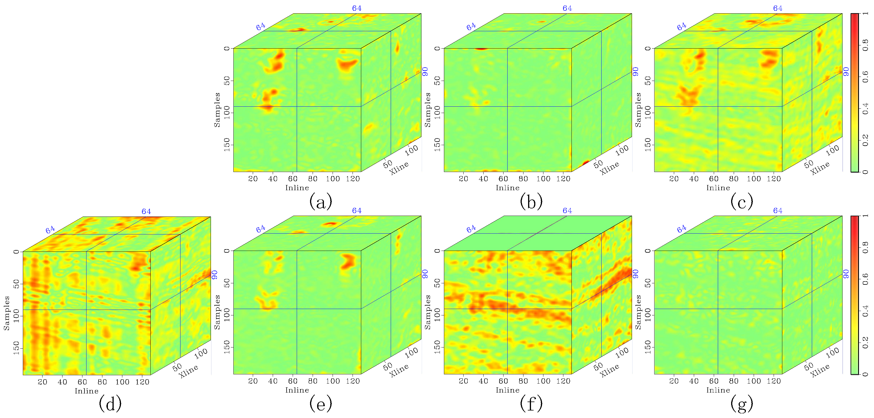
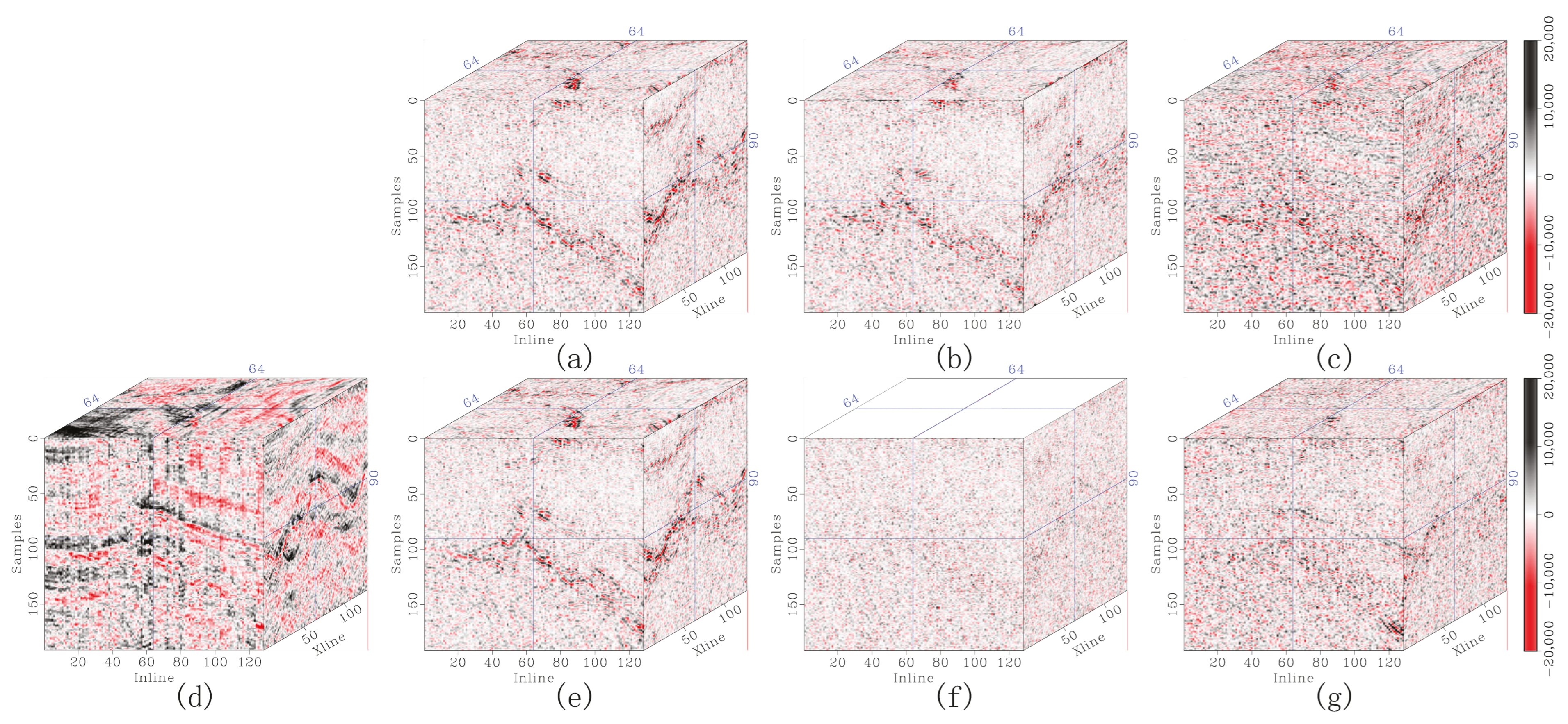
Figure 7.
Local similarity maps of synthetic seismic records with moderate noise contamination using (a) DRR, (b) SOSVMF, (c) SGK, (d) SeisGAN, (e) DIP, (f) PCADDPM, and (g) SSDn-DDPM.
Figure 7.
Local similarity maps of synthetic seismic records with moderate noise contamination using (a) DRR, (b) SOSVMF, (c) SGK, (d) SeisGAN, (e) DIP, (f) PCADDPM, and (g) SSDn-DDPM.
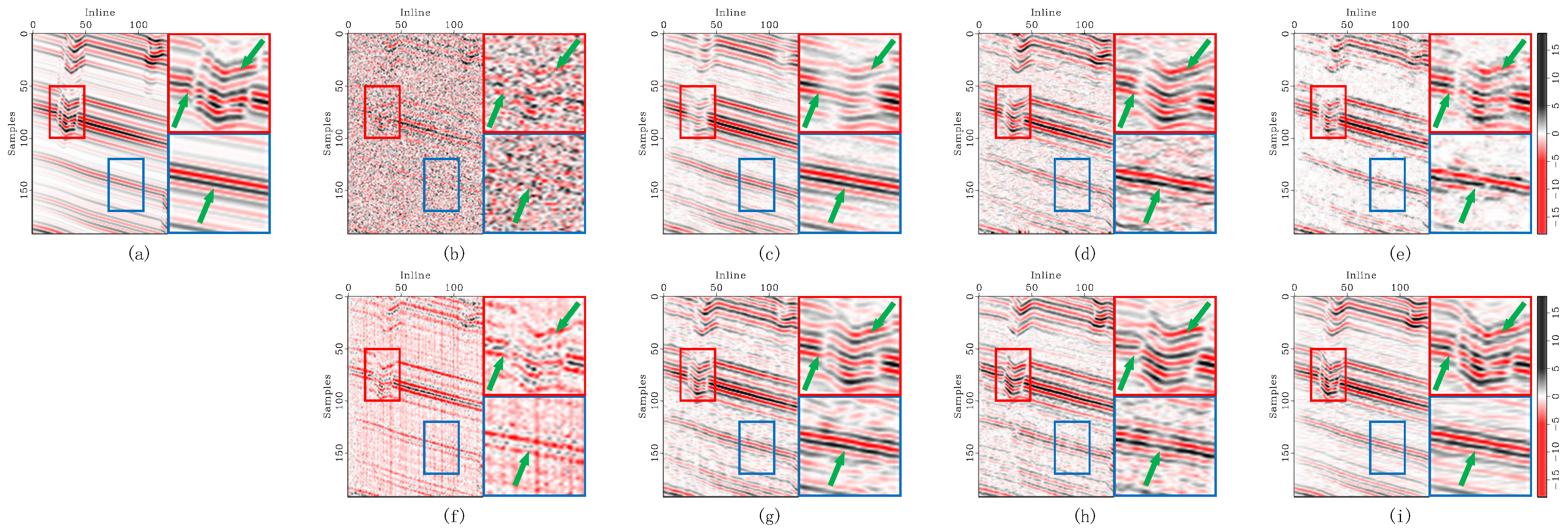
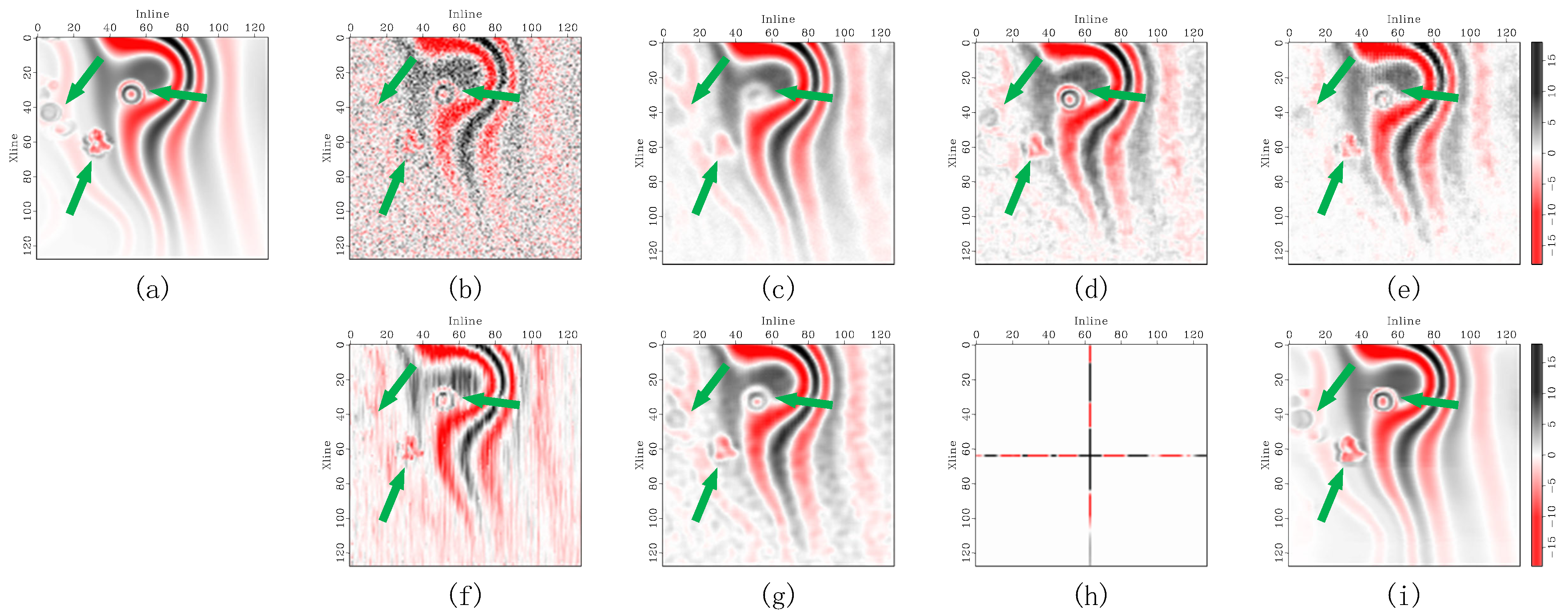
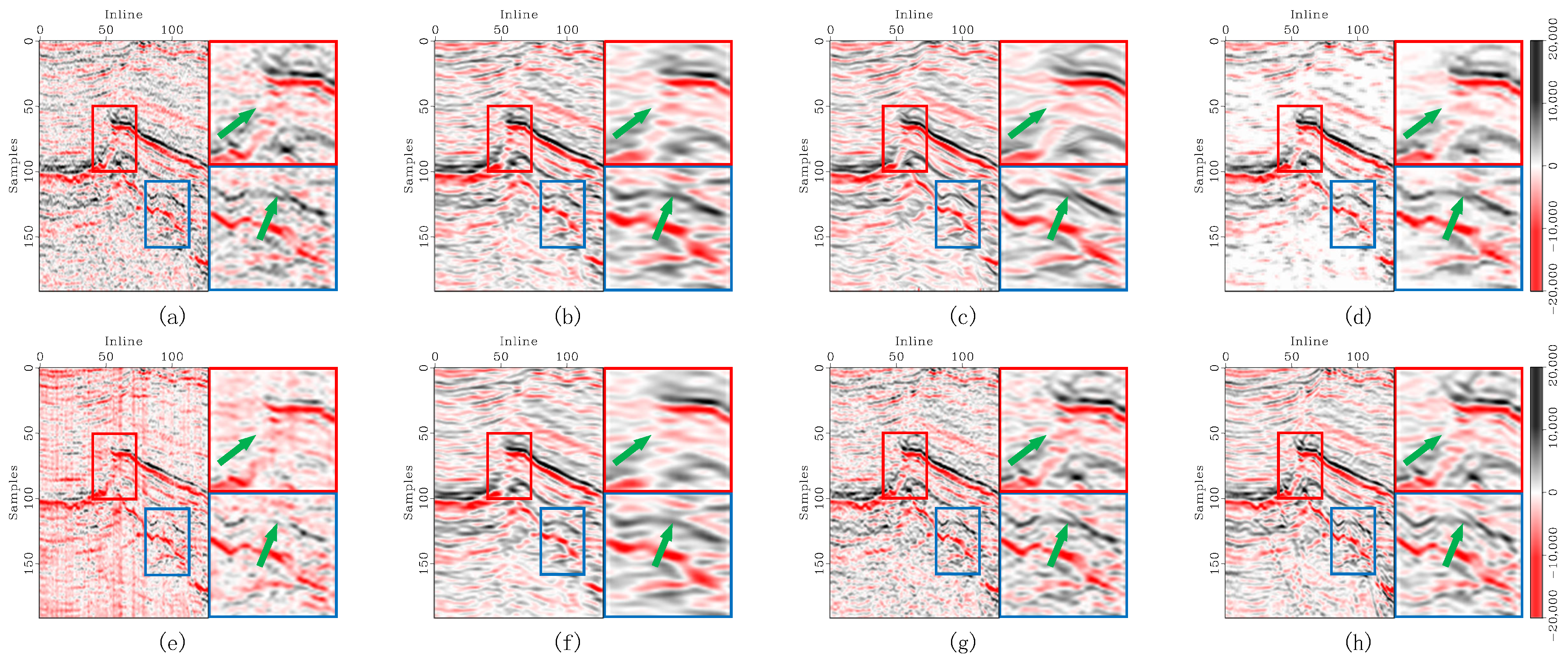
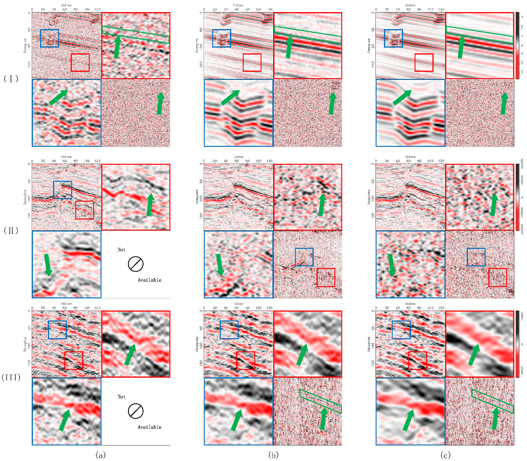
Figure 8.
Enlarged denoising comparison of synthetic seismic inline sections with heavy noise contamination. (a) The original record, (b) noisy data, and denoised data corresponding to (c) DRR, (d) SOSVMF, (e) SGK, (f) SeisGAN, (g) DIP, (h) PCADDPM, and (i) SSDn-DDPM. In each subfigure, the left panel shows the full section, the top-right panel shows the enlarged details of the red-boxed region, and the bottom-right panel shows the enlarged details of the blue-boxed region. Green arrows highlight regions with significant feature differences.
Figure 9.
Denoising comparison of synthetic seismic horizontal slices with heavy noise contamination. (a) The original record, (b) noisy data, and denoised data corresponding to (c) DRR, (d) SOSVMF, (e) SGK, (f) SeisGAN, (g) DIP, (h) PCADDPM, and (i) SSDn-DDPM. Green arrows highlight regions with significant feature differences.
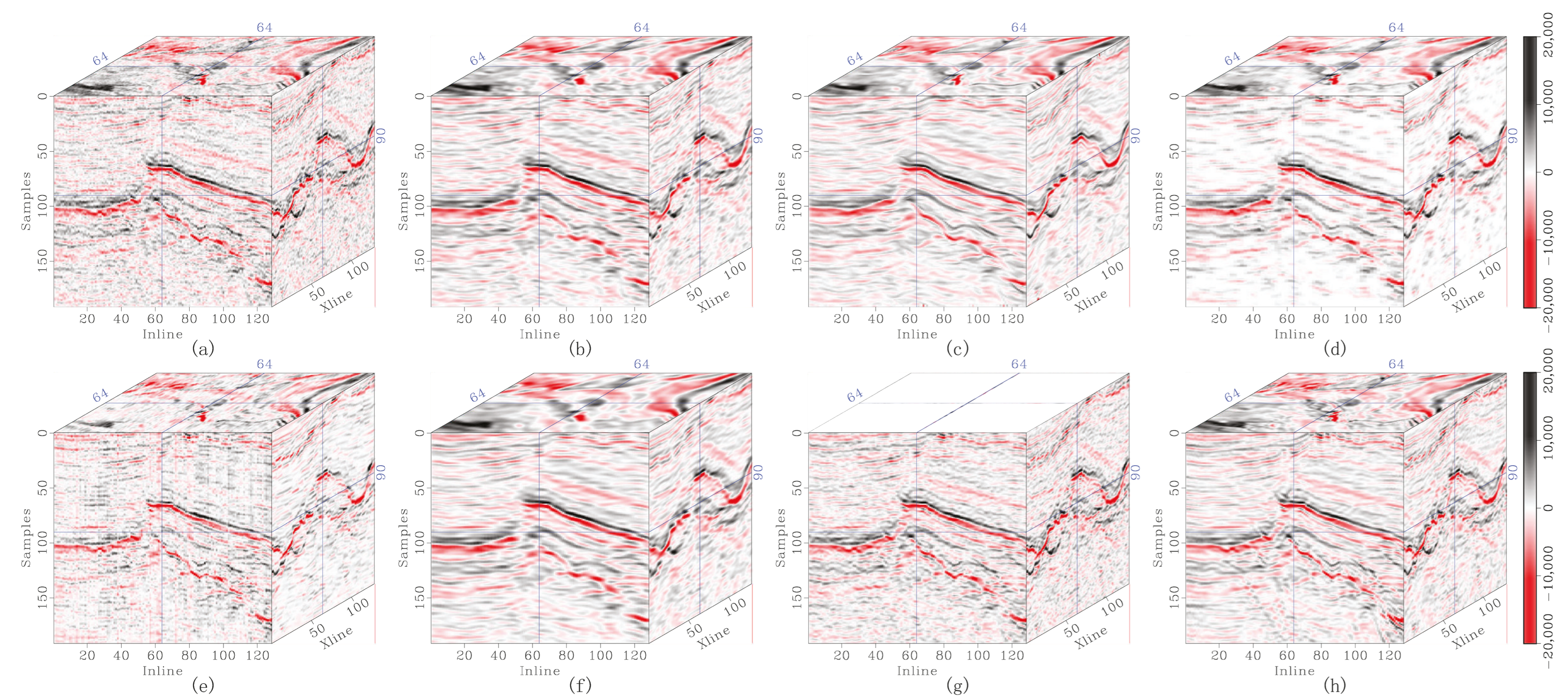
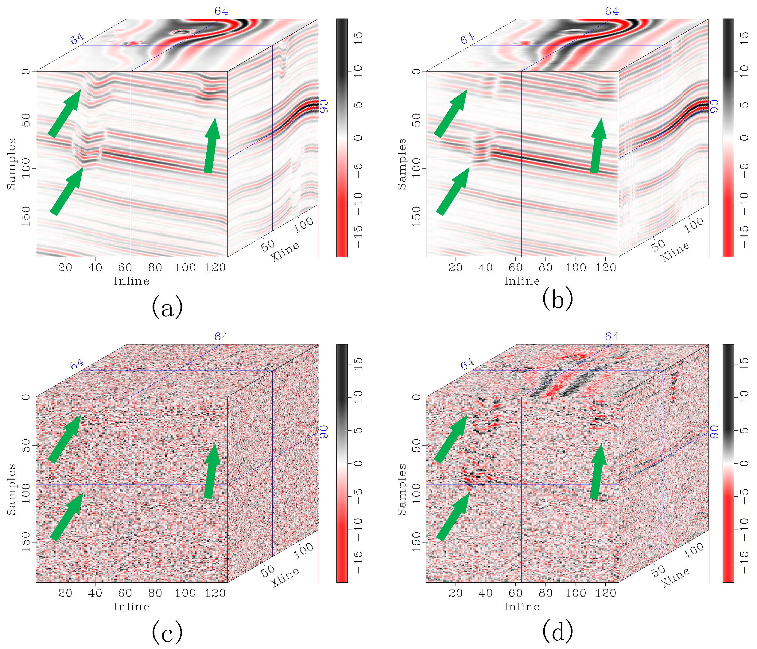
Figure 10.
Denoising comparison in the Stratton 3D seismic data. (a) The original record, and denoised data corresponding to (b) DRR, (c) SOSVMF, (d) SGK, (e) SeisGAN, (f) DIP, (g) PCADDPM, and (h) SSDn-DDPM.
Figure 10.
Denoising comparison in the Stratton 3D seismic data. (a) The original record, and denoised data corresponding to (b) DRR, (c) SOSVMF, (d) SGK, (e) SeisGAN, (f) DIP, (g) PCADDPM, and (h) SSDn-DDPM.
Figure 11.
Comparison of removed noise in the Stratton 3D seismic data. The removed noise corresponding to (a) DRR, (b) SOSVMF, (c) SGK, (d) SeisGAN, (e) DIP, (f) PCADDPM, and (g) SSDn-DDPM.
Figure 11.
Comparison of removed noise in the Stratton 3D seismic data. The removed noise corresponding to (a) DRR, (b) SOSVMF, (c) SGK, (d) SeisGAN, (e) DIP, (f) PCADDPM, and (g) SSDn-DDPM.
Figure 12.
Denoising comparison in the F3 Netherlands seismic data. (a) The original record, and denoised data corresponding to (b) DRR, (c) SOSVMF, (d) SGK, (e) SeisGAN, (f) DIP, (g) PCADDPM, and (h) SSDn-DDPM.
Figure 12.
Denoising comparison in the F3 Netherlands seismic data. (a) The original record, and denoised data corresponding to (b) DRR, (c) SOSVMF, (d) SGK, (e) SeisGAN, (f) DIP, (g) PCADDPM, and (h) SSDn-DDPM.
Figure 13.
Comparison of removed noise in the F3 Netherlands seismic data. The removed noise corresponding to (a) DRR, (b) SOSVMF, (c) SGK, (d) SeisGAN, (e) DIP, (f) PCADDPM, and (g) SSDn-DDPM.
Figure 13.
Comparison of removed noise in the F3 Netherlands seismic data. The removed noise corresponding to (a) DRR, (b) SOSVMF, (c) SGK, (d) SeisGAN, (e) DIP, (f) PCADDPM, and (g) SSDn-DDPM.
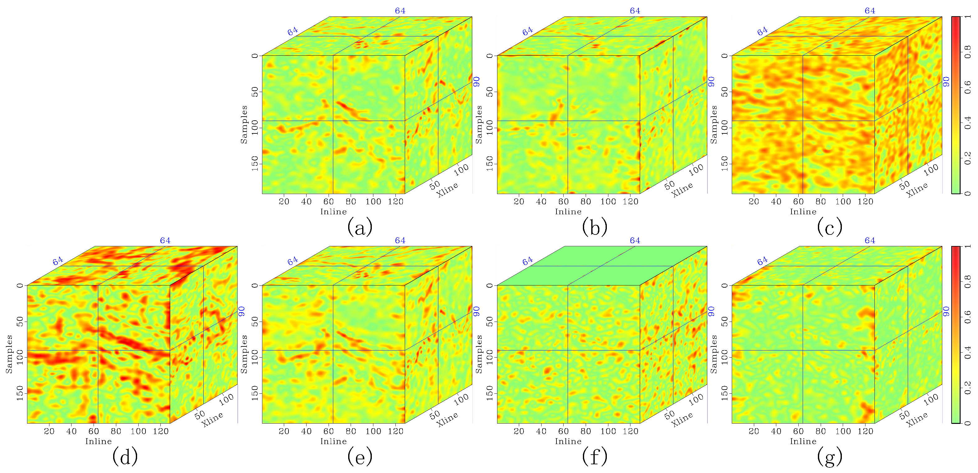
Figure 14.
Local similarity maps of the F3 Netherlands seismic data using (a) DRR, (b) SOSVMF, (c) SGK, (d) SeisGAN, (e) DIP, (f) PCADDPM, and (g) SSDn-DDPM.
Figure 14.
Local similarity maps of the F3 Netherlands seismic data using (a) DRR, (b) SOSVMF, (c) SGK, (d) SeisGAN, (e) DIP, (f) PCADDPM, and (g) SSDn-DDPM.
Figure 15.
Enlarged denoising comparison of the F3 Netherlands seismic data. (a) The original record, and denoised data corresponding to (b) DRR, (c) SOSVMF, (d) SGK, (e) SeisGAN, (f) DIP, (g) PCADDPM, and (h) SSDn-DDPM. In each subfigure, the left panel shows the full section, the top-right panel shows the enlarged details of the red-boxed region, and the bottom-right panel shows the enlarged details of the blue-boxed region. Green arrows highlight regions with significant feature differences.
Figure 16.
Illustration of noise schedule differences. (a) Linear noise schedule. (b) Parameter-freezing noise schedule.
Figure 16.
Illustration of noise schedule differences. (a) Linear noise schedule. (b) Parameter-freezing noise schedule.
Figure 17.
Denoised results with different noise schedules. (a) Denoised result using the parameter-freezing noise schedule. (b) Denoised result using the linear noise schedule. (c) Denoising residual using the parameter-freezing noise schedule. (d) Denoising residual using the linear noise schedule. Green arrows highlight regions with significant feature differences.
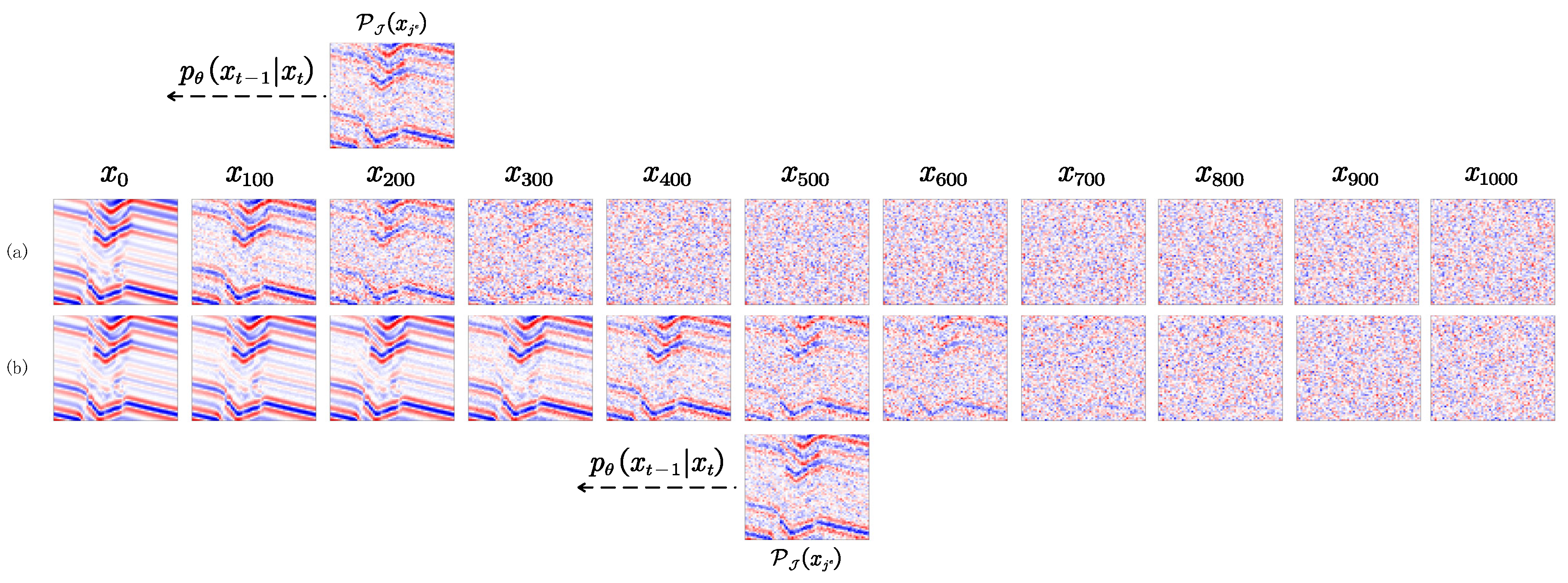
Figure 18.
Illustration of the matching degree between noise-added data sampled from different states in the Markov chain and the noisy input. (a) Data generated from the matched state, specifically the 165th state. (b–e) Data generated from the 300th, 400th, 500th, and 1000th states, respectively. (f) True noisy input. Closer matches indicate better results.
Figure 19.
Ablation experiment removing the seismic noise estimation model. (a) Denoising result obtained with the seismic noise estimation model, sampling from the matched state. (b–e) Denoising results obtained after removing the seismic noise estimation model, sampling from the 300th, 400th, 500th, and 1000th states, respectively. (f) Noiseless ground truth.
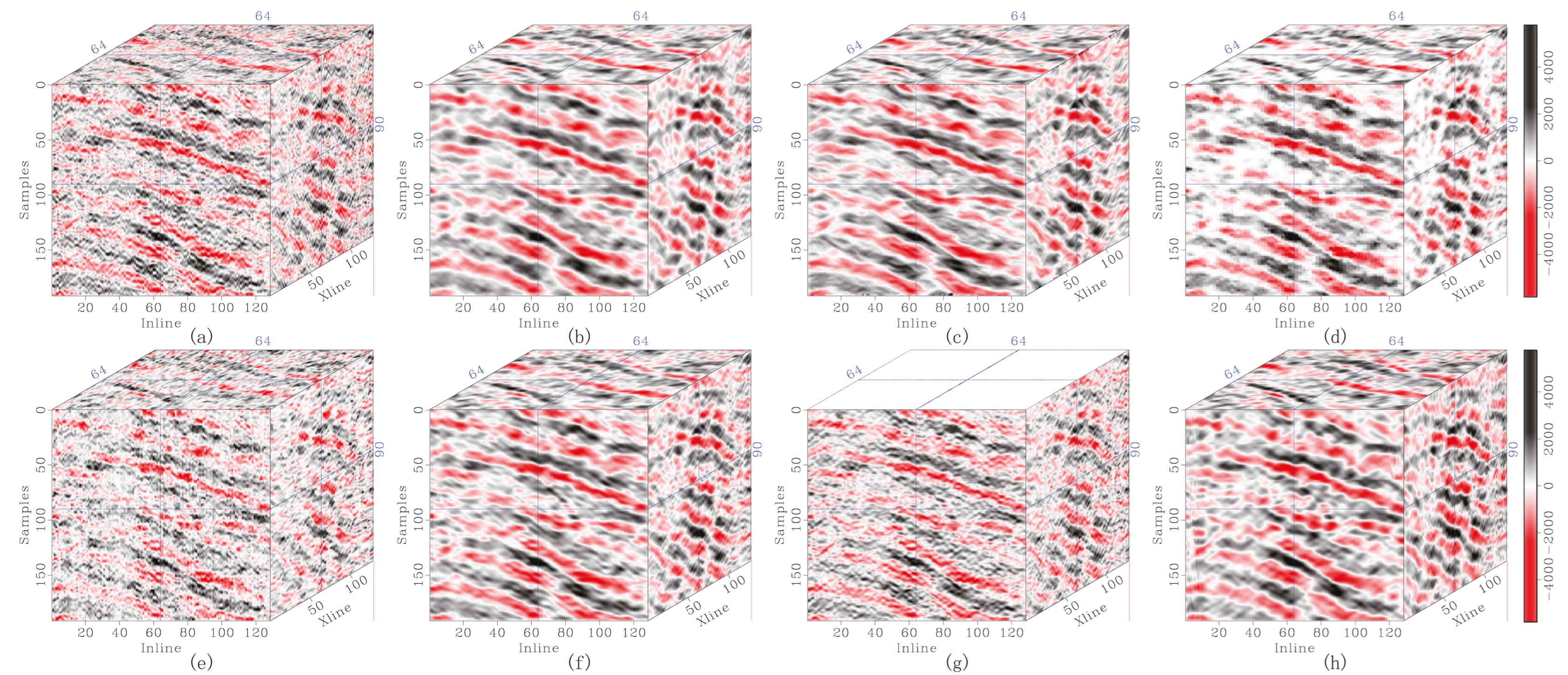
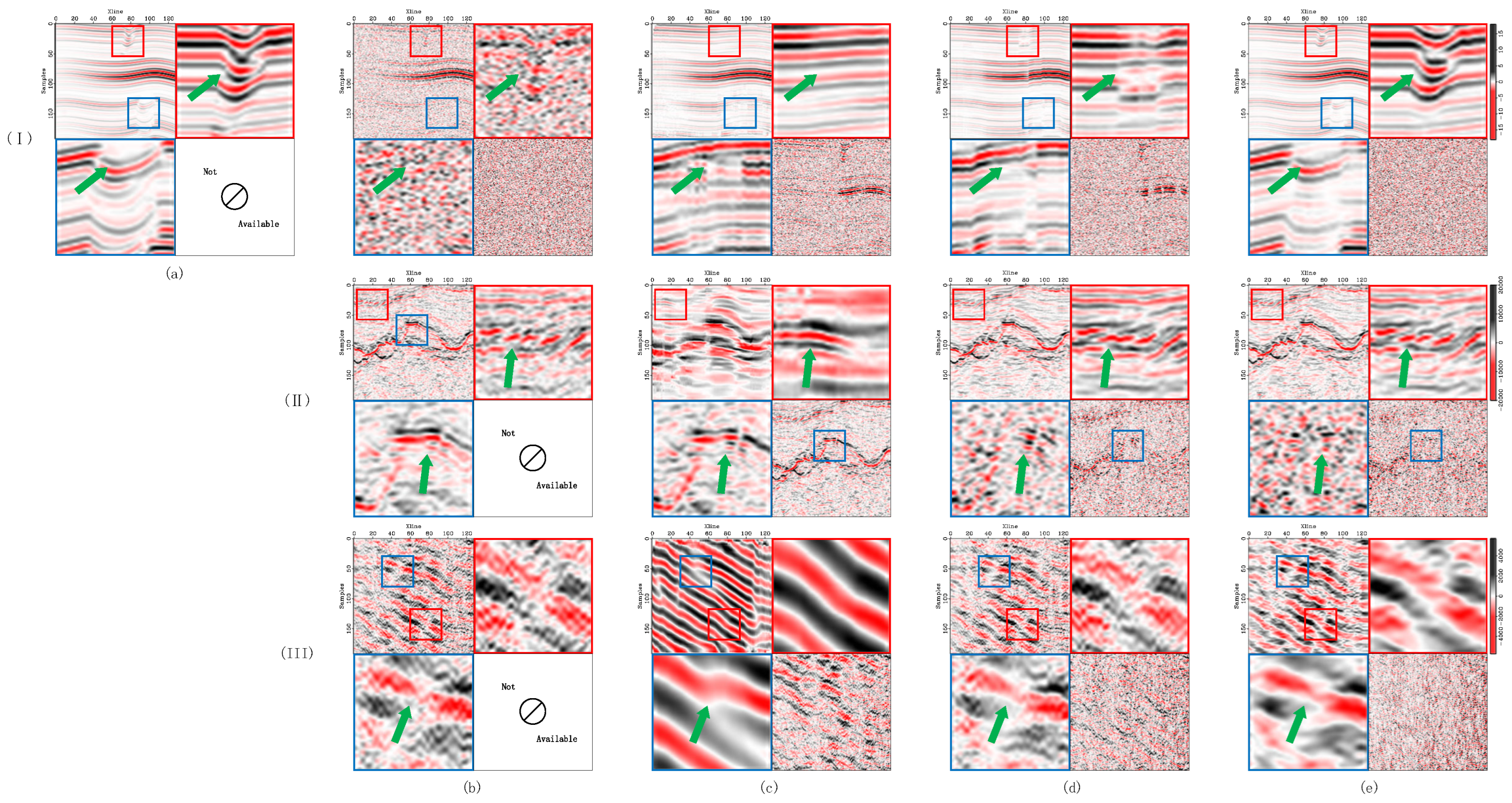
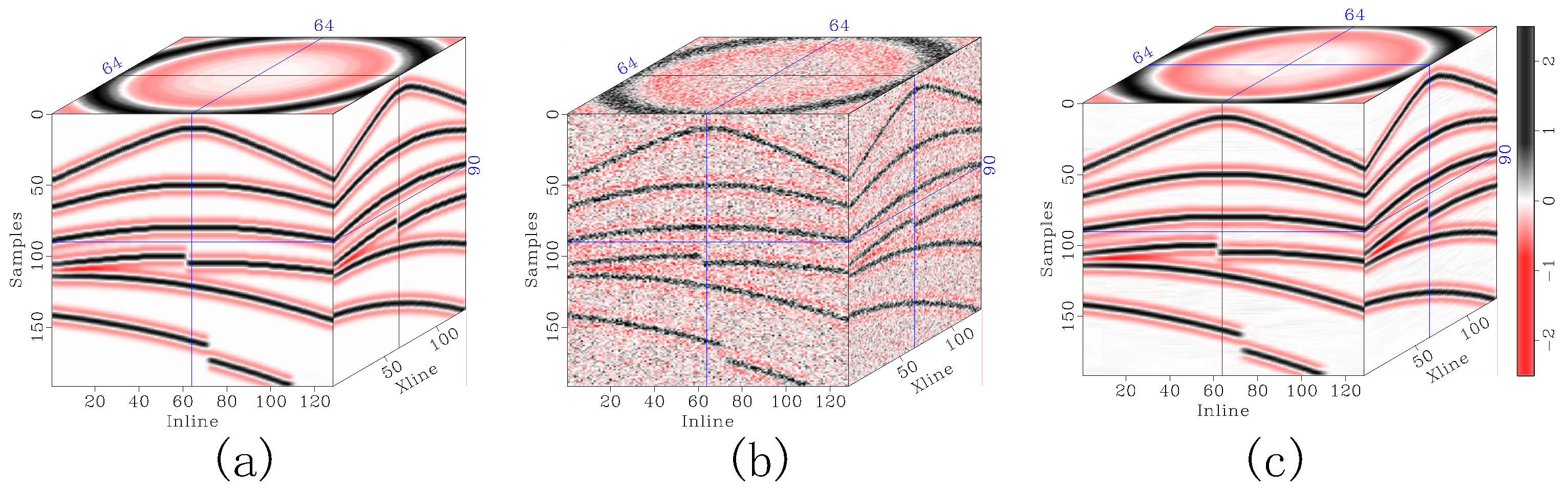
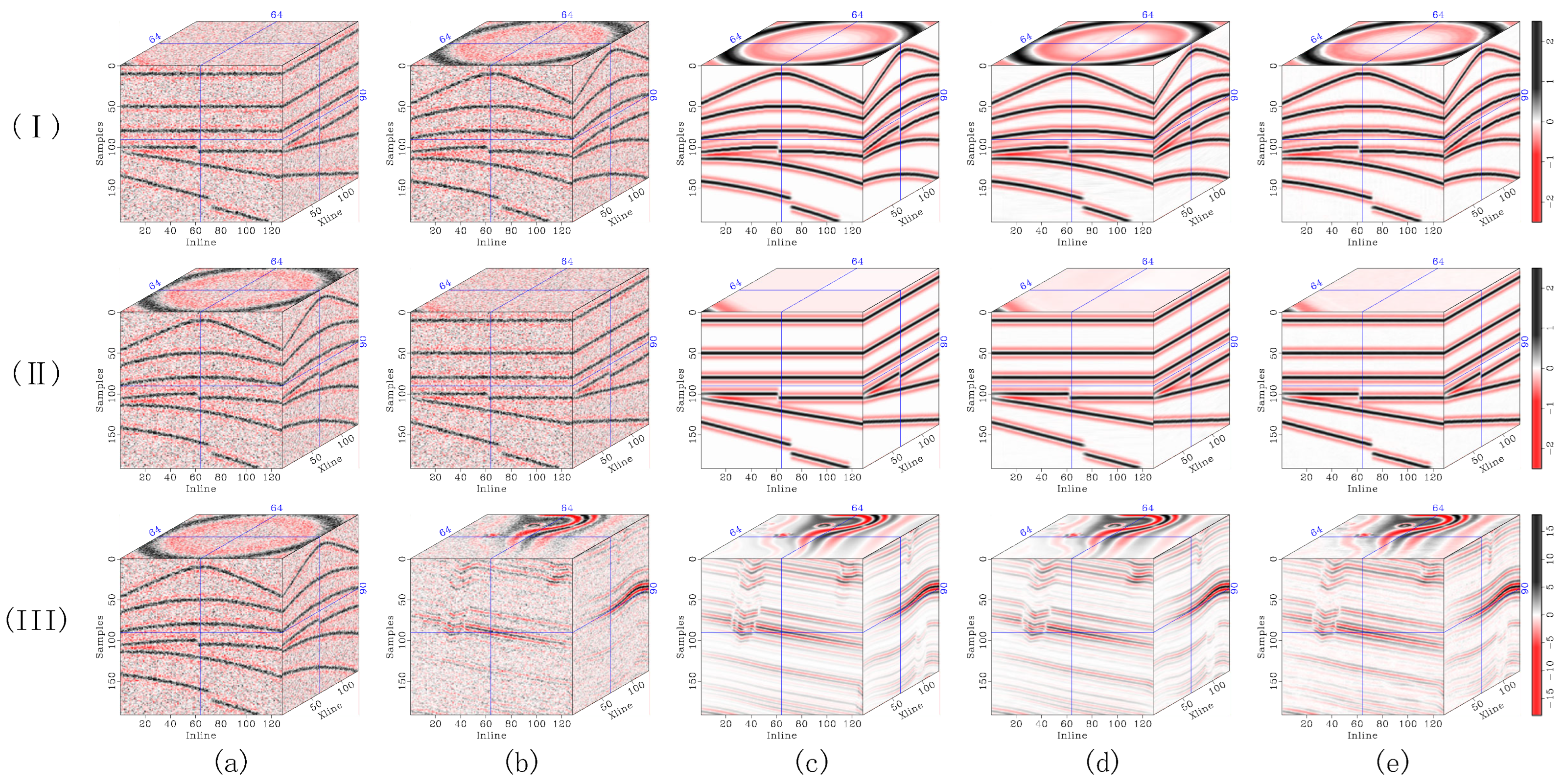
Figure 20.
Ablation experiment replacing 3D serpentine sampling with random sampling and linear-scanning sampling. (I) CigKarst results with moderate noise contamination. (II) Stratton 3D results. (III) F3 Netherlands results. (a) Original record. (b) Noisy data. (c) Denoising results using random sampling. (d) Denoising results using linear-scanning sampling. (e) Denoising results using 3D serpentine sampling. Each subfigure, from top left to bottom right, includes: the full section, enlarged details of the red-boxed region, enlarged details of the blue-boxed region, and the residual corresponding to the full section. Green arrows highlight regions with significant feature differences.
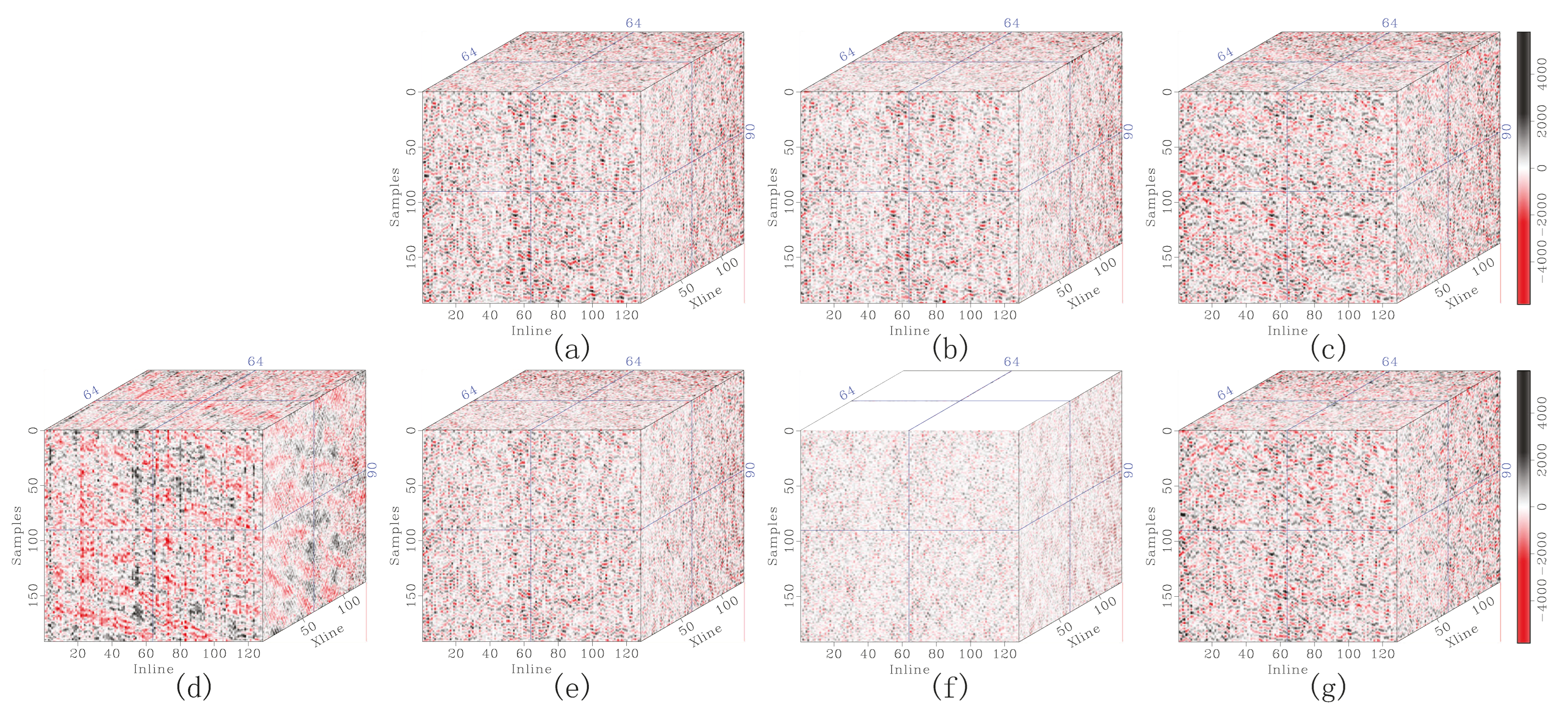
Figure 21.
Ablation experiment removing the diffusion model. (I) CigKarst results with moderate noise contamination. (II) Stratton 3D results. (III) F3 Netherlands results. (a) Noisy data. (b) Denoising results using only the noise distribution estimation model. (c) Complete SSDn-DDPM denoising results. Each subfigure includes, from top left to bottom right, the full section, enlarged details of the red-boxed region, enlarged details of the blue-boxed region, and the residual corresponding to the full section. Green arrows highlight regions with significant feature differences.
Figure 22.
Denoised results of the simple numerical model. (a) Simple numerical model. (b) Noisy simple numerical model. (c) Denoised results of the simple numerical model.
Figure 22.
Denoised results of the simple numerical model. (a) Simple numerical model. (b) Noisy simple numerical model. (c) Denoised results of the simple numerical model.
Figure 23.
Denoised results under different types of noise contamination. (I) Noisy data. (II) Denoised results. (III) Ground truth of noise. (IV) Denoising residual. (a) Impulse noise. (b) Regional noise. (c) Random trace noise. (d) Mixed noise.
Figure 23.
Denoised results under different types of noise contamination. (I) Noisy data. (II) Denoised results. (III) Ground truth of noise. (IV) Denoising residual. (a) Impulse noise. (b) Regional noise. (c) Random trace noise. (d) Mixed noise.
Figure 24.
Denoising results for data with surface wave interference. (a) Pre-stack data. (b) Surface wave interference. (c) Pre-stack data affected by surface wave interference. (d) Denoised pre-stack data affected by surface wave interference. (e) Surface wave and random noise interference. (f) Pre-stack data affected by surface wave and random noise interference. (g) Denoised pre-stack data affected by surface wave and random noise interference.
Figure 25.
Denoised results of the pre-stack and post-stack numerical models. (a) Post-stack model. (b) Noisy post-stack model. (c) Denoised result of the noisy post-stack model. (d) Denoising residual of the noisy post-stack model. (e) pre-stack model. (f) Noisy pre-stack model. (g) Denoised result of the noisy pre-stack model. (h) Denoising residual of the noisy pre-stack model.
Figure 26.
Denoised results of real pre-stack data. (a) Real pre-stack data. (b) Denoised result. (c) Denoising residual.
Figure 26.
Denoised results of real pre-stack data. (a) Real pre-stack data. (b) Denoised result. (c) Denoising residual.
Figure 27.
Comparison of denoising results for model generalization. (I) Pre-stack data test results. (II) Post-stack data test results. (III) CigKarst test results. (a) Training data. (b) Test data. (c) Ground truth of test data. (d) Denoised results under normal usage of the algorithm. (e) Denoised results under generalized usage of the algorithm.
Table 1.
Model parameters.
Table 1.
Model parameters.
| | Noise Prediction Model | Denoising Diffusion Model |
|---|
| Sampling block size | | |
| Sampling stride | | |
| Channel multiplier | 1, 2, 4, 8, 8 | 1, 2, 4, 8, 8 |
| Activation | Swish | Swish |
| Batch size | 32 | 32 |
| Optimizer | Adam | Adam |
| Learning rate | 1 × 10⁻⁴ | 1 × 10⁻⁴ |
| Diffusion steps | - | 1000 |
| Noise schedule | - | (5 × 10⁻⁵, 1 × 10⁻²) |
| Noise schedule freezing ratio | - | 0.2 |
Table 2.
SNR, PSNR, SSIM, MSE, and CS results for synthetic seismic data with light noise contamination. [SNR (dB), PSNR (dB)].
Table 2.
SNR, PSNR, SSIM, MSE, and CS results for synthetic seismic data with light noise contamination. [SNR (dB), PSNR (dB)].
| | SNR | PSNR | SSIM | MSE | CS |
|---|
| Noisy | 4.846 | 24.038 | 0.749 | 0.640 | 0.867 |
| DRR [24,25] | 11.160 | 30.352 | 0.951 | 0.149 | 0.961 |
| SOSVMF [2,68] | 13.346 | 32.538 | 0.960 | 0.090 | 0.976 |
| SGK [20] | 11.600 | 30.792 | 0.927 | 0.135 | 0.967 |
| SeisGAN [40] | 8.119 | 27.070 | 0.913 | 0.318 | 0.917 |
| DIP [60] | 14.612 | 33.803 | 0.979 | 0.067 | 0.982 |
| PCADDPM [48] | 13.595 | 26.580 | 0.942 | 0.131 | 0.980 |
| SSDn-DDPM (Ours) | 16.186 | 35.377 | 0.983 | 0.047 | 0.988 |
Table 3.
SNR, PSNR, SSIM, MSE, and CS results for synthetic seismic data with moderate noise contamination. [SNR (dB), PSNR (dB)].
Table 3.
SNR, PSNR, SSIM, MSE, and CS results for synthetic seismic data with moderate noise contamination. [SNR (dB), PSNR (dB)].
| | SNR | PSNR | SSIM | MSE | CS |
|---|
| Noisy | −1.170 | 20.895 | 0.523 | 2.560 | 0.658 |
| DRR [24,25] | 10.576 | 31.248 | 0.940 | 0.171 | 0.955 |
| SOSVMF [2,68] | 9.613 | 21.760 | 0.876 | 0.213 | 0.945 |
| SGK [20] | 10.143 | 29.348 | 0.917 | 0.189 | 0.952 |
| SeisGAN [40] | 6.171 | 23.398 | 0.837 | 0.820 | 0.801 |
| DIP [60] | 12.843 | 32.046 | 0.955 | 0.101 | 0.973 |
| PCADDPM [48] | 9.698 | 28.454 | 0.890 | 0.752 | 0.951 |
| SSDn-DDPM (Ours) | 14.030 | 33.445 | 0.973 | 0.077 | 0.980 |
Table 4.
SNR, PSNR, SSIM, MSE, and CS results for synthetic seismic data with heavy noise contamination. [SNR (dB), PSNR (dB)].
Table 4.
SNR, PSNR, SSIM, MSE, and CS results for synthetic seismic data with heavy noise contamination. [SNR (dB), PSNR (dB)].
| | SNR | PSNR | SSIM | MSE | CS |
|---|
| Noisy | −5.388 | 17.523 | 0.356 | 6.763 | 0.473 |
| DRR [24,25] | 9.590 | 29.822 | 0.924 | 0.214 | 0.943 |
| SOSVMF [2,68] | 4.268 | 22.619 | 0.594 | 0.731 | 0.833 |
| SGK [20] | 7.845 | 27.500 | 0.853 | 0.321 | 0.915 |
| SeisGAN [40] | 3.160 | 21.145 | 0.724 | 1.820 | 0.673 |
| DIP [60] | 10.200 | 29.391 | 0.905 | 0.186 | 0.951 |
| PCADDPM [48] | 6.564 | 23.578 | 0.766 | 2.995 | 0.901 |
| SSDn-DDPM (Ours) | 10.414 | 30.063 | 0.931 | 0.177 | 0.954 |
Table 5.
Effect of horizontal sampling stride on denoising results. [SNR (dB), PSNR (dB)].
Table 5.
Effect of horizontal sampling stride on denoising results. [SNR (dB), PSNR (dB)].
| | | | | |
|---|
| SNR | 10.225 | 11.609 | 13.422 | 14.030 |
| PSNR | 25.701 | 28.907 | 31.560 | 33.445 |
Table 6.
Effect of diffusion steps on denoising results. [SNR (dB), PSNR (dB)].
Table 6.
Effect of diffusion steps on denoising results. [SNR (dB), PSNR (dB)].
| | Noisy | 200 | 400 | 600 | 800 | 1000 |
|---|
| SNR | 0.099 | 12.203 | 13.414 | 14.054 | 14.291 | 14.276 |
| PSNR | 15.816 | 26.222 | 27.821 | 28.922 | 29.247 | 29.371 |
Table 7.
Processing time comparison of denoising methods. [Time (s)].
Table 7.
Processing time comparison of denoising methods. [Time (s)].
| | SOSVMF | SGK | DRR | SeisGAN | DIP | PCADDPM (2D) | SSDn-DDPM |
|---|
| Average Processing Time | 70,528.14 | 2113.11 | 9841.07 | 225.62 | 233.96 | 11.33 | 1638.81 |
Table 8.
Memory consumption comparison of denoising methods. [MiB].
Table 8.
Memory consumption comparison of denoising methods. [MiB].
| | SOSVMF | SGK | DRR | SeisGAN | DIP | PCADDPM (2D) | SSDn-DDPM |
|---|
| Average Memory Consumption | 389.2 | 819.2 | 1758.4 | 213.4 | 11,889.3 | 67.6 | 1790.9 |
Table 9.
Sampling times when starting from different states. [Time (s)].
Table 9.
Sampling times when starting from different states. [Time (s)].
| | 165th (Matched State) | 500th | 1000th |
|---|
| Time | 3.017 | 7.649 | 14.612 |
Table 10.
SNR, PSNR, SSIM, MSE, and CS results for different sampling methods. [SNR (dB), PSNR (dB)].
Table 10.
SNR, PSNR, SSIM, MSE, and CS results for different sampling methods. [SNR (dB), PSNR (dB)].
| | SNR | PSNR | SSIM | MSE | CS |
|---|
| Noisy | 4.846 | 24.038 | 0.749 | 0.640 | 0.867 |
| −1.170 | 20.895 | 0.523 | 2.560 | 0.658 |
| −5.388 | 17.523 | 0.356 | 6.763 | 0.473 |
| Random Sampling | 6.105 | 25.297 | 0.894 | 0.479 | 0.873 |
| 3.683 | 22.874 | 0.792 | 0.837 | 0.759 |
| 2.872 | 22.064 | 0.694 | 1.009 | 0.701 |
| Linear-Scanning Sampling | 7.405 | 26.597 | 0.922 | 0.355 | 0.907 |
| 6.236 | 25.464 | 0.906 | 0.465 | 0.880 |
| 9.145 | 29.451 | 0.911 | 0.238 | 0.938 |
| 3D Serpentine Sampling | 16.186 | 35.377 | 0.983 | 0.047 | 0.988 |
| 14.030 | 33.445 | 0.973 | 0.077 | 0.980 |
| 10.414 | 30.063 | 0.931 | 0.177 | 0.954 |
Table 11.
SNR, PSNR, SSIM, MSE, and CS results w/o the diffusion model. [SNR (dB), PSNR (dB)].
Table 11.
SNR, PSNR, SSIM, MSE, and CS results w/o the diffusion model. [SNR (dB), PSNR (dB)].
| | SNR | PSNR | SSIM | MSE | CS |
|---|
| Noisy | 4.846 | 24.038 | 0.749 | 0.640 | 0.867 |
| −1.170 | 20.895 | 0.523 | 2.560 | 0.658 |
| −5.388 | 17.523 | 0.356 | 6.763 | 0.473 |
| w/o Diffusion Model | 10.611 | 32.239 | 0.906 | 0.089 | 0.973 |
| 9.466 | 31.528 | 0.871 | 0.115 | 0.967 |
| 6.479 | 28.435 | 0.739 | 0.230 | 0.937 |
| Complete SSDn-DDPM | 16.186 | 35.377 | 0.983 | 0.047 | 0.988 |
| 14.030 | 33.445 | 0.973 | 0.077 | 0.980 |
| 10.414 | 30.063 | 0.931 | 0.177 | 0.954 |
Table 12.
Denoising results of post-stack and pre-stack data. [SNR (dB), PSNR (dB)].
Table 12.
Denoising results of post-stack and pre-stack data. [SNR (dB), PSNR (dB)].
| | Post-Stack Data | Pre-Stack Data |
|---|
| | Noisy | Denoised | Noisy | Denoised |
|---|
| SNR | −0.539 | 24.551 | −0.596 | 24.080 |
| PSNR | 17.818 | 39.344 | 17.783 | 38.827 |
Table 13.
Comparison of denoising results between generalized and conventional model applications. [SNR (dB), PSNR (dB), SSIM].
Table 13.
Comparison of denoising results between generalized and conventional model applications. [SNR (dB), PSNR (dB), SSIM].
| | Testing Data | Post-Stack Data | Pre-Stack Data |
|---|
| Training Data | |
|---|
| Post-Stack Data | 24.551 | 39.344 | 0.971 | 23.853 | 37.526 | 0.959 |
| Pre-Stack Data | 24.855 | 39.386 | 0.975 | 24.080 | 38.827 | 0.963 |


 ,
, 
