Detecting Lunar Subsurface Water Ice Using FMCW Ground Penetrating Radar: Numerical Analysis with Realistic Permittivity Variations

Abstract

This study investigates the detectability of a putative layer of regolith containing water ice in the lunar polar regions using ground penetrating radar (GPR). Numerical simulations include realistic variations in the relative permittivity of the lunar regolith, considering both density and, for the first time, the effects of temperature on permittivity profiles. We follow the case of previous theoretical studies of water migration, which suggest that water ice accumulates at depths ranging from a few centimeters to tens of centimeters, appropriate depths to explore using GPR. In particular, frequency-modulated continuous wave (FMCW) radar is well-suited for this purpose due to its high range resolution and robust signal-to-noise ratio. This study evaluates two scenarios for the presence of lunar water ice: (1) a layer of regolith containing water ice at a depth of 5 cm, with a thickness of 5 cm, and (2) a layer of regolith containing water ice at a depth of 20 cm, with a thickness of 10 cm. Our computational results show that FMCW GPR, equipped with a dynamic range of 90 dB, is capable of detecting reflections from the interfaces of these layers, even under conditions of low water ice content and using antennas with low directivity. In addition, optimized antenna offsets improve the resolution of the upper and lower interfaces, particularly when applied to the surface of ancient crater ejecta. This study highlights the critical importance of understanding subsurface density and temperature structures for the accurate detection of water-ice-bearing regolith layers.

1. Introduction

Recent observations of the lunar polar regions suggest the potential presence of water ice with a wide range of ice contents, from less than 1.0 wt% [1,2,3] to as much as about 30 wt% [4]. However, the exact forms and the amounts of water ice still remain unresolved. Theoretical studies have shown that the dynamics of water molecule accumulation in lunar subsurface layers is strongly influenced by the thermal and physical properties of the regolith [5,6]. These studies highlight the importance of understanding the subsurface environment at depths of tens of centimeters to meters, where diurnal and seasonal temperature variations drive water migration and form concentration peaks in cold-trapping environments. Understanding these processes is critical to elucidating the mechanisms governing water retention and migration on the Moon.

Ground penetrating radar (GPR) is a well-established technique for investigating subsurface layers at these depths. For example, lunar penetrating radar (LPR) was successfully used in the Chang’e missions [7,8], and future missions, including LUnar Polar EXploration (LUPEX), are expected to employ similar techniques [9]. Frequency-modulated continuous wave (FMCW) is one of the most suitable GPR methods for planetary exploration due to its ability to achieve a high resolution and signal-to-noise ratio over long distances. FMCW uses broadband signals with time-varying frequencies that improve penetration depth and range resolution. This approach has been demonstrated by RIMFAX, the GPR onboard NASA’s Perseverance rover, which has shown its utility in planetary subsurface exploration [10]. For depths relevant to this study, a frequency range of 0.5–3.0 GHz provides an optimal balance between penetration depth and vertical resolution, as planned for use in the WISDOM instrument on the ExoMars rover, designed for Martian water ice exploration [11].

The effectiveness of GPR depends on the relative permittivity profile of the subsurface material. However, evaluations based on terrestrial conditions may not be directly applicable to the lunar subsurface, given its lack of atmosphere, extreme temperatures, and dry regolith. Numerical analysis thus becomes essential for accurately assessing GPR performance under lunar conditions. Accurate numerical modeling requires proper parameterization of the relative permittivity profile. Importantly, laboratory studies suggest that permittivity depends on factors such as density, temperature, frequency, and chemical composition, with temperature dependence being particularly important for lunar conditions [12]. Previous numerical studies have often oversimplified permittivity models by assuming constant values [13,14,15], employing linear variations [16,17], or by using the density-dependent model of ε_r = 1.919^ρ [18,19,20] introduced by Heiken et al. (1991) [21]. However, significant density and temperature variations in the lunar subsurface may require accurate modeling.

In this study, we aim to evaluate the detectability of subsurface regolith layers containing water ice using 0.5–3.0 GHz FMCW radar, incorporating realistic density and temperature-dependent permittivity variations in the lunar polar regions where subsurface water sequestration occurs. We also compare these results to those obtained under the simplified assumption of constant permittivity, providing a benchmark for assessing the importance of incorporating more nuanced permittivity profiles.

2. Materials and Methods

2.1. Assumptions of Subsurface Structure on the Moon

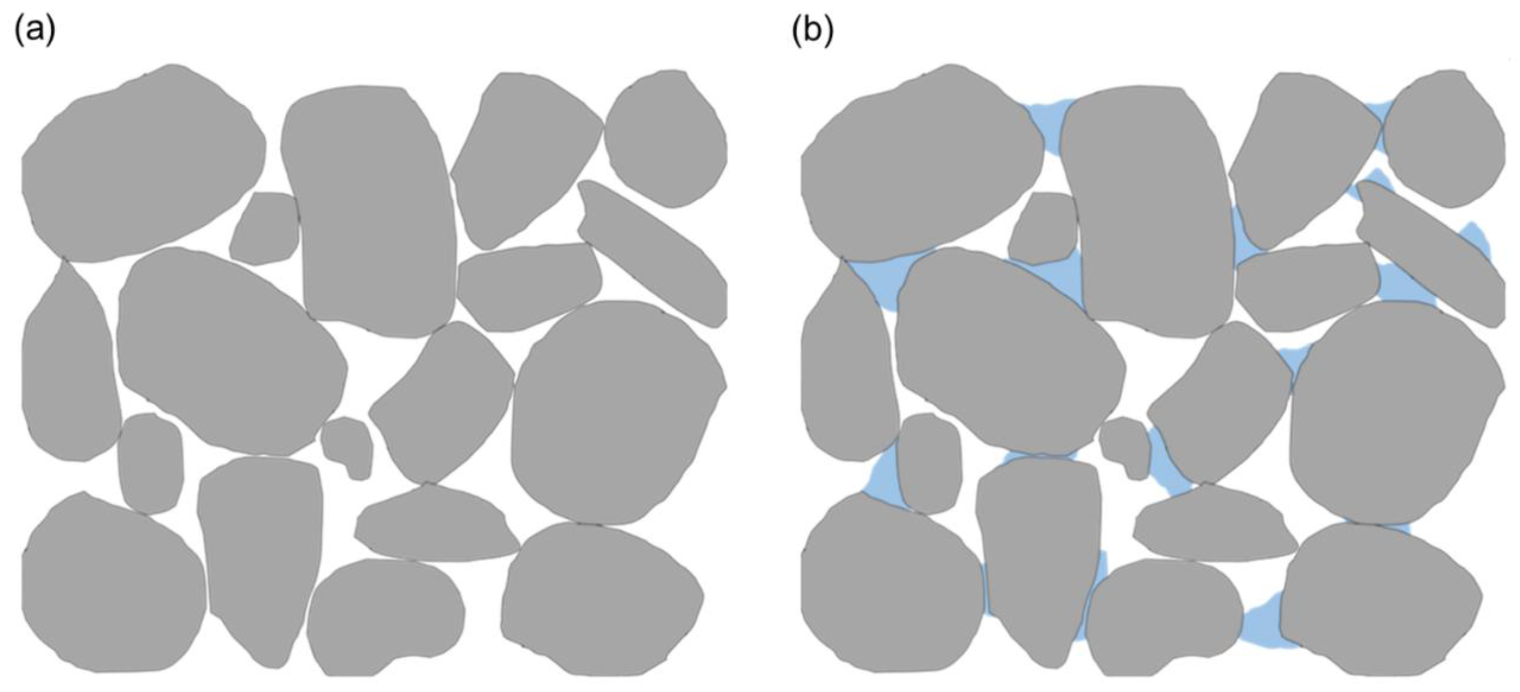
2.1.1. Possible Conditions of Regolith and Water Ice

The exact forms and states of water ice on the Moon remain uncertain; however, water migration models [5,6] suggest that a layer of regolith containing water ice underlies a desiccation layer on the order of a few centimeters in thickness. Reiss et al. (2021) [5] estimate that water accumulation occurs at depths of several centimeters below the surface and could extend to approximately 50 cm on a 1 Ga timescale. Similarly, Schorghofer (2022) [6], focusing on the lunar south polar region near 85° latitude, predicts that over a 100 kyr timescale, a layer of regolith containing water ice several centimeters thick forms at a depth of approximately 5 cm beneath the surface. Over 1 Ga, this layer of regolith containing water ice could grow to several decimeters in thickness at a depth of around 20 cm, with water ice content reaching up to 1 wt%.

This study considers two scenarios based on these insights: (1) a layer of regolith containing water ice at a depth of 5 cm, with a thickness of 5 cm, and (2) a layer of regolith containing water ice at a depth of 20 cm, with a thickness of 10 cm. In both scenarios, the water ice content is assumed to be 0.5 wt%, reflecting a rather conservative state, which is challenging to detect.

Measurements from the Kaguya Spectral Profiler, calibrated with LOLA data [22], have shown that the regolith composition at the lunar south pole is predominantly anorthositic. This is consistent with findings suggesting that pure anorthosite regions (PANs) are widely distributed across the Moon, including its south pole [23]. Based on these observations, this study assumes that the regolith is entirely composed of anorthosite.

The density profile of the lunar subsurface can be derived from the following equation, which describes the relationship between depth and density [24]:

$$\rho ={\rho }_d-\left({\rho }_d-{\rho }_s\right)\exp \left(-{\displaystyle \frac{z}{H}}\right)$$

(1)

where z is the depth, ρ_s = 1.1 g/cm³ and ρ_d = 1.8 g/cm³ represent the density at the surface and at depths much greater than the H-parameter, respectively. The H-parameter, adjusted for a latitude of 85°, is set to 0.2 m [25]. In addition, we calculated the subsurface temperature profile at 85° latitude using the thermal conductivity model for lunar regolith at low temperatures, developed by Martinez and Siegler (2021) [26], which is particularly suitable for accurate estimations in the cold, high-latitude regions of the Moon. Density and temperature profiles are shown in Figure 1.

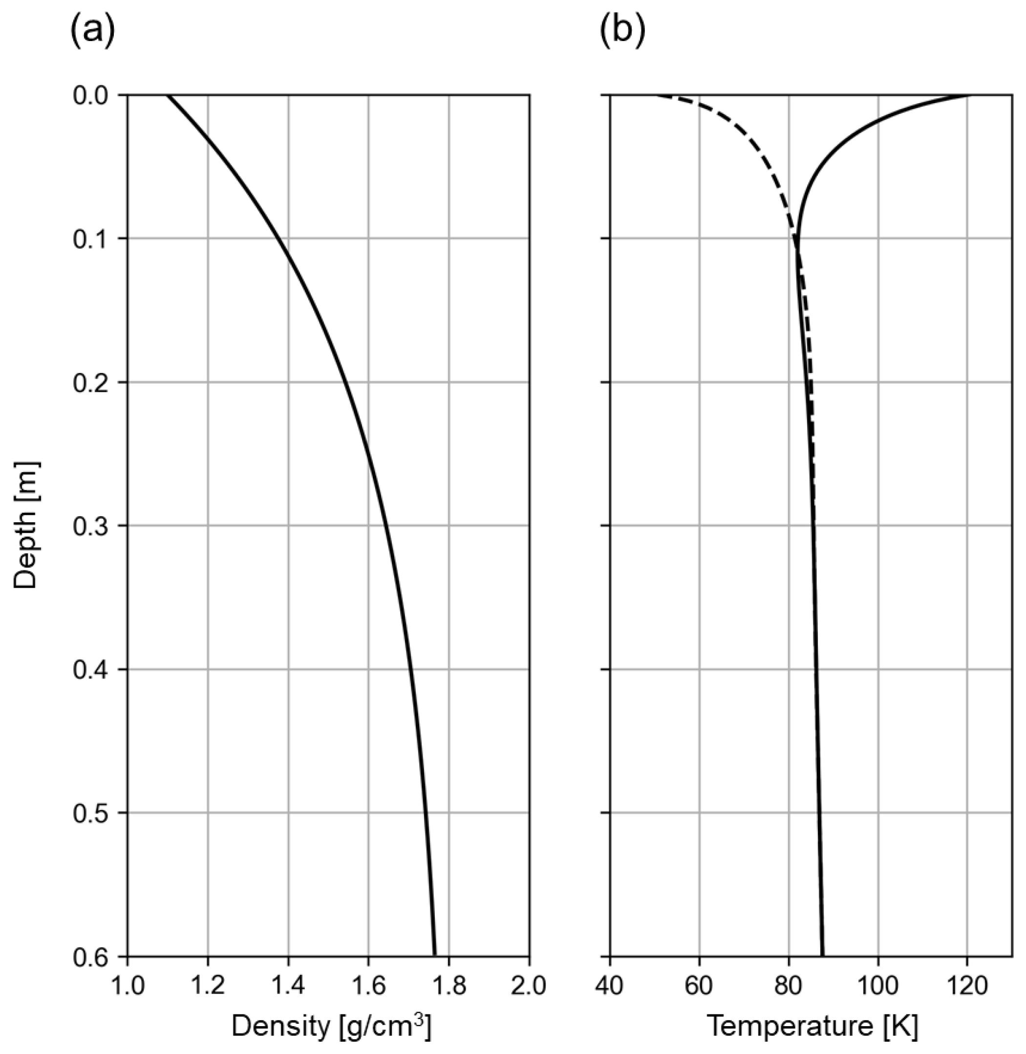
2.1.2. Electromagnetic Properties of Subsurface Materials

Numerical analysis of electromagnetic wave propagation requires the accurate characterization of material properties, including relative permittivity, conductivity, relative permeability, and magnetic loss. In this study, relative permeability and magnetic loss are assigned values of 1 and 0, respectively, as the materials considered are non-magnetic. The electrical conductivity of the regolith, on the other hand, varies depending on factors such as FeO and TiO₂ content and temperature, with estimated values ranging from 10⁻¹⁴ S/m to 1.5 × 10⁻³ S/m [27,28]. Although the electrical conductivity of the lunar surface layer is generally considered to be low, a conservative value of 1.5 × 10⁻³ S/m is used in this study to examine the detectability, even when higher-loss material or basaltic components are locally present, which represents challenging conditions.

The dominant factor affecting electromagnetic wave propagation is relative permittivity. For its calculation, the Landau–Lifshitz–Looyenga (LLL) mixing rule [29] is used, as follows:

$${\epsilon }^{{\displaystyle \frac{1}{3}}}=v_1{{\epsilon }_1}^{{\displaystyle \frac{1}{3}}}+\left(1-v_1\right){{\epsilon }_2}^{{\displaystyle \frac{1}{3}}}$$

(2)

Here, ε represents the permittivity of the mixture, while ε₁ and ε₂ are the relative permittivities of its components, with v₁ denoting the volume fraction. Assuming that regolith is a mixture of anorthosite particles and voids, the bulk permittivity (ε_bulk) can be written as

$${{\epsilon }_{bulk}}^{{\displaystyle \frac{1}{3}}}=v_{grain}{{\epsilon }_{grain}}^{{\displaystyle \frac{1}{3}}}+\left(1-v_{grain}\right){{\epsilon }_{void}}^{{\displaystyle \frac{1}{3}}}$$

(3)

where ε_grain and ε_void are the relative permittivities of the anorthosite particles and voids (i.e., ε_void = 1), respectively. The volume fraction of the anorthosite particles in the regolith, v_grain, can be expressed as

$$v_{grain}={\displaystyle \frac{{\rho }_{bulk}}{{\rho }_{grain}}}$$

(4)

where ρ_bulk and ρ_grain represent the bulk density of the regolith and the grain density of anorthosite, respectively. Therefore, to calculate ε_bulk, it is necessary to determine ρ_bulk, ρ_grain, and ε_grain. For ρ_bulk, we directly use the density profile calculated in Equation (1). The values of ρ_grain and ε_grain are obtained from the experimental measurement research [12], where the relative permittivity of anorthosite with a porosity of 40% was measured at 20 °C, −20 °C, and −60 °C over the frequency range of 2 GHz to 6 GHz. These measurements established that the grain density of the anorthosite particles is 2.645 g/cm³. Furthermore, at 2 GHz, the measured permittivity exhibited a linear relationship with temperature, as follows:

$${\epsilon }_{40\%\_2\mathrm{G}\mathrm{H}\mathrm{z}}\left(T\right)=0.0052T+2.9437$$

(5)

where T is the temperature in degrees Celsius. Consequently, ε_grain(T) can be obtained by substituting ε_bulk = ε_{40%_2GHz}(T), v_grain = 0.6, and ε_void = 1 into Equation (3) as a function of T. Using the determined values of ρ_bulk, ρ_grain, and ε_grain, we can finally calculate ε_bulk from Equation (3), which depends on both the density and the temperature.

The relative permittivity of water ice used in this study is determined to be 3.11, extrapolating the result of the laboratory measurement [30] to the target temperature. This value is also consistent with the reported value of 3.1, which shows minimal temperature dependence at significantly low temperatures [31].

Subsequently, the approach for calculating the relative permittivity of a regolith and water ice mixture is outlined. As illustrated in Figure 2a, we assume that dry regolith consists solely of anorthosite particles and voids. In the regolith layer containing water ice, it is assumed that water ices occupy the voids between the anorthosite particles, as demonstrated in Figure 2b. Therefore, the relative permittivity of the regolith and water ice mixture can be determined using the LLL mixing rule introduced in Equation (2), as follows:

$${{\epsilon }_{mixture}}^{{\displaystyle \frac{1}{3}}}=v_{grain}{{\epsilon }_{grain}}^{{\displaystyle \frac{1}{3}}}+\left(1-v_{grain}\right){{\epsilon }_{ice+void}}^{{\displaystyle \frac{1}{3}}}$$

(6)

Here, ε_mixture and ε_ice+void represent the relative permittivity of the entire mixture and that of the water ice/void component, respectively. In turn, ε_ice+void can be expressed as

$${{\epsilon }_{ice+void}}^{{\displaystyle \frac{1}{3}}}={\displaystyle \frac{v_{ice}}{1-v_{grain}}}{{\epsilon }_{ice}}^{{\displaystyle \frac{1}{3}}}+{\displaystyle \frac{1-v_{grain}-v_{ice}}{1-v_{grain}}}{{\epsilon }_{void}}^{{\displaystyle \frac{1}{3}}}$$

(7)

where ε_ice is the relative permittivity of water ice, which is defined to be 3.11, and v_ice is the volume fraction of water ice, given by

$$v_{ice}={\displaystyle \frac{{\rho }_{bulk}}{{\rho }_{ice}}}{\displaystyle \frac{w}{1-w}}$$

(8)

Here, ρ_bulk = 0.94 g/cm³ is the density of water ice, measured by the flotation method at temperatures between 82 K and 110 K [32], and w denotes the mass fraction of water ice (i.e., w = 0.005). Therefore, by applying Equations (4), (7) and (8), Equation (6) can be rewritten as follows:

$$\begin{gathered} {{\epsilon }_{mixture}}^{{\displaystyle \frac{1}{3}}}={\displaystyle \frac{{\rho }_{bulk}}{{\rho }_{grain}}}{{\epsilon }_{grain}}^{{\displaystyle \frac{1}{3}}}+{\displaystyle \frac{{\rho }_{bulk}}{{\rho }_{ice}}}{\displaystyle \frac{w}{1-w}}{{\epsilon }_{ice}}^{{\displaystyle \frac{1}{3}}} \\ \hspace{1em}\hspace{1em}\hspace{1em}\hspace{1em}\hspace{1em}\hspace{1em}\hspace{1em}+\left(1-{\displaystyle \frac{{\rho }_{bulk}}{{\rho }_{grain}}}-{\displaystyle \frac{{\rho }_{bulk}}{{\rho }_{ice}}}{\displaystyle \frac{w}{1-w}}\right){{\epsilon }_{void}}^{{\displaystyle \frac{1}{3}}} \end{gathered}$$

(9)

Finally, to calculate ε_mixture from Equation (9), the density profile calculated in Equation (1) is used as the value for ρ_bulk, while the previously calculated value for the relative permittivity of the dry regolith is used to determine ε_grain.

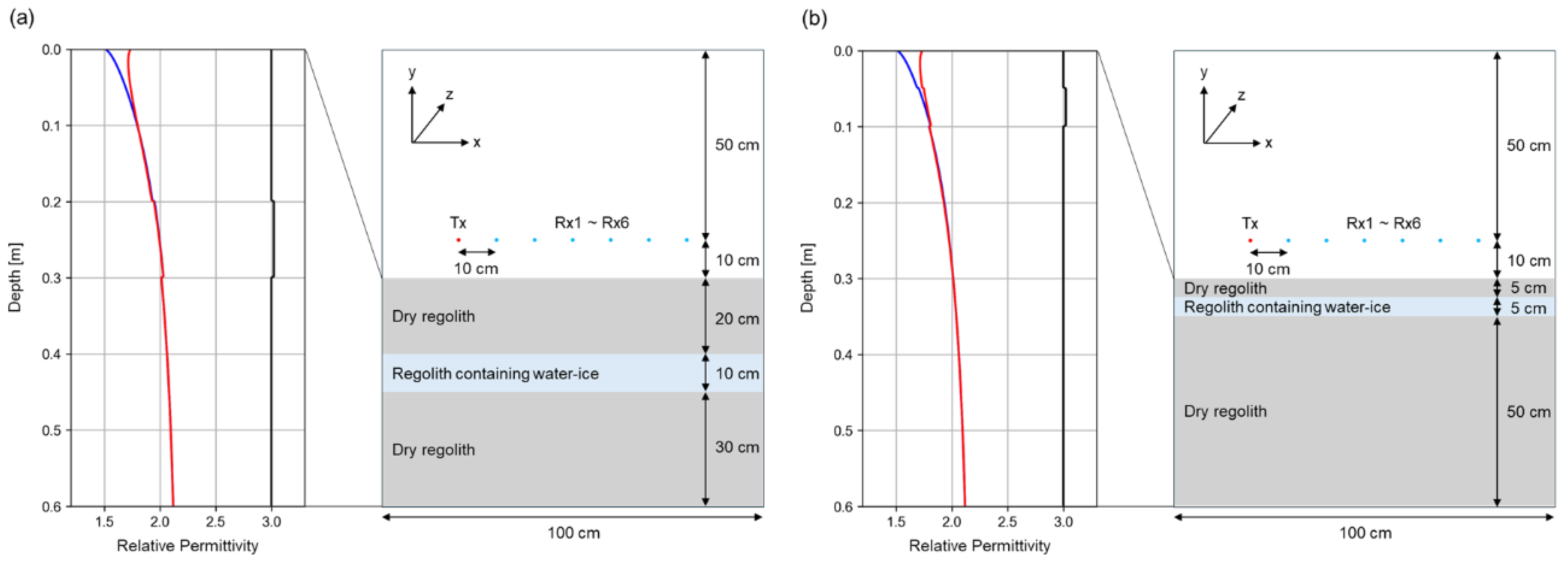
2.2. Simulation Setup and Geometry

In this study, the finite-difference time-domain (FDTD) method is adopted because of its suitability for broadband analysis. The FDTD method calculates the E and H components of electromagnetic waves alternately at half-time steps on a cubic mesh called a Yee cell [33]. The calculations are performed using the open-source software gprMax (v3.1.5) [34], distributed under the GNU General Public License version 3.0. Based on the FDTD method, gprMax solves Maxwell’s equations in three dimensions using the transverse electromagnetic (TEM) mode. The conditions and parameters used in the simulations are shown in

Table 1. Conditions and parameter settings used in the simulations.

Parameter	Setting
Total simulation space	1.0 × 1.2 × 1.0 m3
Spatial discretization ∆x, ∆y, and ∆z	2 mm
Temporal discretization ∆t	3.85167 ps 1
Absorbing boundary conditions	Perfectly matched layer (PML) 2
Antenna	Hertzian dipole antenna
Antenna offset from the ground	10 cm
Offsets between Tx and Rxs	10–60 cm (10 cm interval)
Frequency band	0.5–3.0 GHz 3
Pulse duration	50 µs

¹ The value is calculated at the Courant–Friedrichs–Lewy (CFL) limit. ² PMLs are applied to all six surfaces of the simulation domain, with a thickness of 20 mm. ³ The input signal consists of a chirp wave.

.

The schematic diagrams of the geometries and corresponding relative permittivity profiles are shown in Figure 3. The gradual variation of the relative permittivity calculated by Equation (9) is introduced in both the dry layer and the layer containing 0.5 wt% water ice. To incorporate this layered structure, we discretize the subsurface with a 2 mm vertical step (corresponding to our FDTD cell size) and assign a spatially varying permittivity to each cell. From Figure 3, it is clear that in every scenario, the layer containing water ice exhibits a higher permittivity than that of the adjacent dry layers. Furthermore, a noticeable difference emerges in the permittivity structure between daytime and nighttime, which is consistent with previous research indicating that lunar permittivity varies with local time, based on remote sensing data [35]. These conditions, characterized by a low water ice content and the use of a low-directivity antenna, are selected to examine the feasibility of detecting a layer of regolith containing water ice under challenging scenarios.

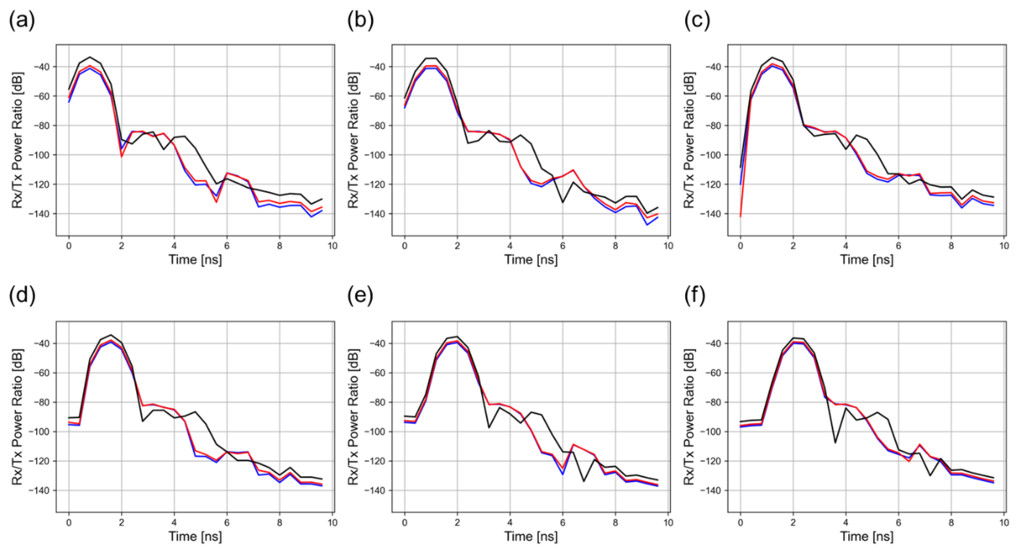
2.3. Signal Processing

The signal processing methodology employed in this study uses established FMCW radar techniques to isolate subsurface reflection signals by suppressing extraneous components, including direct wave interference. The process consists of several steps designed to enhance the clarity of target reflections while minimizing interfering signal components.

First, background signals, including direct wave interference, are removed. These background signals are pre-recorded and serve as references for subtraction, simulating the acquisition of reference data in the orbital environment, as performed by lunar regolith penetrating radar (LRPR) [36]. This step suppresses non-target reflections, isolating weaker and delayed signals originating from the lunar subsurface.

Next, the cleaned reflection signals are mixed with a reference waveform derived from the transmitted chirp signal. This process generates an intermediate frequency signal, or beat frequency, which encodes temporal information related to the depth and structure of the subsurface layers. The resulting beat signal is then passed through a low-pass filter with a cutoff frequency of 500 kHz to remove high-frequency noise. This cutoff frequency is chosen based on the radar’s maximum expected beat frequency for near-surface investigations, which in our configuration, corresponds to about 500 kHz for a two-way travel time of 10 ns. By discarding extraneous high-frequency components, the filter enhances the signal-to-noise ratio and preserves the reflection signals critical for subsurface analysis.

Additionally, a Blackman window is applied to minimize spectral leakage and reduce interference from the side lobes. This windowing step enhances the precision of frequency-domain analysis, isolating distinct reflection signals from the subsurface layers. Following this, a fast Fourier transform (FFT) is performed to convert the windowed signal from the time domain to the frequency domain, enabling the extraction of beat frequency components. The beat frequencies are then scaled using the sweep duration-to-bandwidth ratio (T/B) to interpret them as depth-related time intervals, providing insights into the structure of the lunar subsurface.

Finally, intensity calibration is performed to account for variations in antenna positioning and mixing process gains. This step ensures the accurate estimation of received signal intensity by comparing the processed signals to a calibration reference derived from a geometry involving only the antennas. This calibrated approach provides reliable intensity estimates for the analyzed signals.

After these procedures, the first major reflection in the processed data typically arises from the lunar surface, given that direct waves are removed by background subtraction. Subsequent reflections appear from the upper and lower interfaces of a water-ice-bearing layer, followed by weaker signals resulting from multiple reflections at various interfaces. Observing the characteristic amplitudes, delays, and spacing of these peaks can provide evidence for the potential presence of water ice.

3. Results and Discussion

Figure 4 shows the results for antenna offsets ranging from 10 cm to 60 cm, under the assumption that a layer of regolith containing water ice with a thickness of 10 cm is located at a depth of 20 cm beneath the surface. The first peak is attributed to the reflection from the surface of the regolith, while the two subsequent peaks are indicative of reflections from the top and bottom interfaces of the water-ice-containing regolith layer, respectively. The subsequent peaks are interpreted as the results of multiple reflections within the structure. In Figure 4, the horizontal axis is the time in nanoseconds, which corresponds to distance by considering the electromagnetic wave propagation velocity in the medium. The surface reflection appears at around 1–2 ns, and the peaks corresponding to the water-ice-bearing layer are observed at about 2–5 ns.

Peaks corresponding to theoretical values are observed across all cases at Rx/Tx power ratios in the range of about –90 dB to –80 dB, even under the assumption of a low water ice content and low-directivity antennas. Accordingly, a dynamic range of 90 dB is necessary to adequately characterize the reflections from the layer of regolith containing water ice. Under the assumption of a constant relative permittivity of 3, the upper and lower interfaces of the layer containing water ice can be distinguished. However, when a more realistic, depth-dependent permittivity is introduced, the individual interfaces become more difficult to observe, even though the overall reflection amplitude is enhanced. This outcome stems from two main factors. First, the overall permittivity of the regolith becomes lower than 3 at many depths, while the water ice permittivity remains 3.11, resulting in a larger dielectric contrast at the water ice boundary and thereby increasing the total reflection amplitude. Second, because the average permittivity is lower, the electromagnetic waves travel faster in the regolith, causing a reduction in two-way travel times. Reflections from multiple interfaces are consequently compressed and can overlap, making it more challenging to distinguish each boundary clearly. Therefore, although the overall signal strength benefits from a higher contrast at the water ice boundary, the compressed arrival times introduce complexities that hinder the clear identification of individual interfaces. In multi-static radar configurations, if reflections from both the upper and lower interfaces of the layer of regolith containing water ice can be clearly distinguished, it may enable the estimation of the relative permittivity of the layer, based on the cross-correlation of the traces in a CMP gather [37], and consequently, the water ice content. While this difference is most pronounced under the assumption of a constant relative permittivity of 3 for the regolith, regardless of depth, it remains observable for an antenna offset of 10 cm, even when the relative permittivity is modeled to vary gradually with depth, taking into account density and temperature changes.

Subsequently, Figure 5 shows the results plotted for a scenario in which a layer of regolith containing water ice with a thickness of 5 cm is assumed to exist at a depth of 5 cm below the surface. Across all scenarios, no significant differences are observed, and the reflection from the layer of regolith containing water ice is obscured by the stronger reflection from the regolith surface. To address this, additional calculations are performed for a scenario in which no layer of regolith containing water ice exists, i.e., where the subsurface consists solely of dry regolith. By using this as a background and removing it, the reflection from the regolith surface is eliminated, allowing the reflections from the layer of regolith containing water ice to be isolated. This approach is analogous to the mean subtraction method, one of the most commonly used background removal techniques in GPR. The results of this analysis are shown in Figure 6.

The peaks appearing at about 1–3 ns represent reflections from the layer containing water ice. Although the proximity of this layer to the surface and its thinness make detection more difficult, these reflections are still discernible once the strong surface reflection is eliminated by background subtraction with the dynamic range of 90 dB across all antenna offsets. However, distinguishing the top and bottom interfaces of the water-ice-bearing layer remains challenging when considering the realistic permittivity profile. Nevertheless, the ability to detect this layer under such conditions is considered sufficient for site-screening purposes in missions such as, potentially, LUPEX, PRIME-1, and Chang’e series missions (and WISDOM on Mars), in which drilling or sampling could be prioritized in areas where subsurface water ice is implicated [38]. On the other hand, there is a minimal difference between daytime and nighttime conditions.

The lunar surface has been subjected to numerous impacts of varying scales, forming craters and depositing ejecta that are thought to have created complex stratigraphic structures. This process is considered significant in the polar regions as well, where recent studies have investigated ejecta thickness, its role in protecting water ice from impacts, and proposed landing sites for future exploration based on these factors [39,40,41]. Within this context, we focus on the potential application of GPR in future exploration, suggesting that if a layer of regolith containing water ice is present, it can be detected, even when located on the ejecta of relatively young craters, such as those formed 100 kyr ago. Furthermore, for ejecta originating from craters over 1 Ga, careful determination of antenna offsets could allow for the distinction between the upper and lower interfaces of the layer of regolith containing water ice. These findings demonstrate the feasibility of using GPR to investigate putative water ice on the lunar subsurface in polar regions.

Although our simulations focus on a uniformly anorthositic regolith with two representative scenarios, lunar regolith can contain FeO- and TiO₂-rich phases and rock fragments of varying sizes, potentially influencing dielectric properties and scattering. Moreover, water ice may also occur at depths, thicknesses, and concentrations beyond those modeled here; deeper or lower-content layers could yield weaker reflected signals due to increased attenuation; shallower layers may be more difficult to distinguish from strong surface echoes, and thinner layers can produce faint or overlapping reflections that complicate boundary identification. Exploring such variations would increase computational complexity but could refine our understanding of GPR detectability and will be addressed in future work. Furthermore, while the present study uses a low-directivity antenna to represent a conservative detection scenario, antennas with higher directivities or gains could enhance signal-to-noise ratios and provide additional design references for real GPR missions. Comparing our numerical approach with existing lunar GPR data is still challenging, given incomplete knowledge of local ground truth, but new observations will help validate and improve future simulations. Although we have relied on modeling here, laboratory experiments and field tests with lunar simulants under cryogenic conditions could also serve as important steps toward experimental verification.

4. Conclusions

This study demonstrates the ability of FMCW ground penetrating radar to detect subsurface layers containing water ice under realistic lunar conditions, including gradual variations in relative permittivity due to density and temperature changes. Our results confirm that reflections from both the upper and lower interfaces of a regolith layer containing water ice are detectable, even in challenging scenarios with the presence of ice displaying only a very low water ice content (0.5 wt%), by using low-directivity antennas, requiring a dynamic range of 90 dB. These results indicate that GPR for shallow subsurface exploration in the lunar polar regions can provide valuable insights into volatile retention and migration processes.

Furthermore, the ability to resolve layer interfaces on crater ejecta, even in young craters (100 kyr), and to distinguish older structures with optimized antenna configurations underscores the robustness of this approach. This highlights the potential of GPR to advance our understanding of lunar subsurface structures and support future exploration missions.

Future work could focus on the experimental validation of these results, the refinement of antenna design, and the deployment of FMCW GPR during upcoming missions such as LUPEX. Such efforts will further enhance the potential of radar systems to unravel the mysteries of lunar water ice distribution and its implications for sustained exploration.

References

1. Pieters, C.M.; Goswami, J.N.; Clark, R.N.; Annadurai, M.; Boardman, J.; Buratti, B.; Combe, J.-P.; Dyar, M.D.; Green, R.; Head, J.W.; et al. Character and spatial distribution of OH/H2O on the surface of the Moon seen by M3 on Chandrayaan-1. Science 2009, 326, 568–572. [Google Scholar] [CrossRef] [PubMed]
2. Miller, R.S.; Nerurkar, G.; Lawrence, D.J. Enhanced hydrogen at the lunar poles: New insights from the detection of epithermal and fast neutron signatures. J. Geophys. Res. Planets 2012, 117, E11007. [Google Scholar] [CrossRef]
3. Sanin, A.B.; Mitrofanov, I.G.; Litvak, M.L.; Bakhtin, B.N.; Bodnarik, J.G.; Boynton, W.V.; Chin, G.; Evans, L.; Harshman, K.; Fedosov, F.; et al. Hydrogen distribution in the lunar polar regions. Icarus 2017, 283, 20–30. [Google Scholar] [CrossRef]
4. Li, S.; Lucey, P.G.; Milliken, R.E.; Hayne, P.O.; Fisher, E.; Williams, J.P.; Hurley, D.M.; Elphic, R.C. Direct evidence of surface exposed water ice in the lunar polar regions. Proc. Natl. Acad. Sci. USA 2018, 115, 8907–8912. [Google Scholar] [CrossRef]
5. Reiss, P.; Warren, T.; Sefton-Nash, E.; Trautner, R. Dynamics of subsurface migration of water on the Moon. J. Geophys. Res. Planets 2021, 126, e2020JE006742. [Google Scholar] [CrossRef]
6. Schorghofer, N. Gradual sequestration of water at lunar polar conditions due to temperature cycles. Astrophys. J. Lett. 2022, 927, L34. [Google Scholar] [CrossRef]
7. Lai, J.; Xu, Y.; Bugiolacchi, R.; Meng, X.; Xiao, L.; Xie, M.; Liu, B.; Di, K.; Zhang, X.; Zhou, B.; et al. First look by the Yutu-2 rover at the deep sub-surface structure at the lunar farside. Nat. Commun. 2020, 11, 3426. [Google Scholar] [CrossRef] [PubMed]
8. Su, Y.; Fang, G.Y.; Feng, J.Q.; Xing, S.G.; Ji, Y.C.; Zhou, B.; Gao, Y.-Z.; Li, H.; Dai, S.; Xiao, Y.; et al. Data processing and initial results of Chang’e-3 lunar penetrating radar. Res. Astron. Astrophys. 2014, 14, 1623–1632. [Google Scholar] [CrossRef]
9. Prajapati, V.; Kumar, B.S.; Kumar, P.; Agrawal, R.A.; Rao, C.V.N. Design and Implementation of Equivalent Time Sampling Scheme on FPGA for Impulse GPR. In Proceedings of the 2024 IEEE Space, Aerospace and Defence Conference (SPACE), Bangalore, India, 22–23 July 2024; pp. 207–210. [Google Scholar] [CrossRef]
10. Hamran, S.E.; Paige, D.A.; Amundsen, H.E.; Berger, T.; Brovoll, S.; Carter, L.; Damsgård, L.; Dypvik, H.; Eide, J.; Eide, S.; et al. Radar imager for Mars’ subsurface experiment—RIMFAX. Space Sci. Rev. 2020, 216, 128. [Google Scholar] [CrossRef]
11. Ciarletti, V.; Corbel, C.; Plettemeier, D.; Cais, P.; Clifford, S.M.; Hamran, S.E. WISDOM GPR designed for shallow and high-resolution sounding of the Martian subsurface. Proc. IEEE 2011, 99, 824–836. [Google Scholar] [CrossRef]
12. Kobayashi, M.; Miyamoto, H.; Pál, B.D.; Niihara, T.; Takemura, T. Laboratory measurements show temperature-dependent permittivity of lunar regolith simulants. Earth Planets Space 2023, 75, 8. [Google Scholar] [CrossRef]
13. Dai, S.; Su, Y.; Xiao, Y.; Feng, J.Q.; Xing, S.G.; Ding, C.Y. Echo simulation of lunar penetrating radar: Based on a model of inhomogeneous multilayer lunar regolith structure. Res. Astron. Astrophys. 2014, 14, 1642–1653. [Google Scholar] [CrossRef]
14. Xiao, Y.; Su, Y.; Dai, S.; Feng, J.; Xing, S.; Ding, C.; Li, C. Ground experiments of Chang’e-5 lunar regolith penetrating radar. Adv. Space Res. 2019, 63, 3404–3419. [Google Scholar] [CrossRef]
15. Putrevu, P.; Pandey, D.K.; Chakraborty, T. GPR Sensitivity Analysis for Detection of Subsurface Layers in Lunar Scenario. In Proceedings of the 2021 IEEE MTT-S International Microwave and RF Conference (IMARC), Kanpur, India, 17–19 December 2021; pp. 1–4. [Google Scholar] [CrossRef]
16. Fa, W. Modeling and simulation for ground penetrating radar study of the subsurface structure of the moon. In Proceedings of the 2012 14th International Conference on Ground Penetrating Radar (GPR), Shanghai, China, 4–8 June 2012; pp. 922–926. [Google Scholar] [CrossRef]
17. Fa, W. Simulation for ground penetrating radar (GPR) study of the subsurface structure of the Moon. J. Appl. Geophys. 2013, 99, 98–108. [Google Scholar] [CrossRef]
18. Zhang, L.; Zeng, Z.F.; Li, J.; Lin, J.Y. Study on regolith modeling and lunar penetrating radar simulation. In Proceedings of the 2016 16th International Conference on Ground Penetrating Radar (GPR), Hong Kong, China, 13–16 June 2016; pp. 1–5. [Google Scholar] [CrossRef]
19. Zhang, L.; Zeng, Z.; Li, J.; Lin, J.; Hu, Y.; Wang, X.; Sun, X. Simulation of the lunar regolith and lunar-penetrating radar data processing. IEEE J. Sel. Top. Appl. Earth Obs. Remote Sens. 2018, 11, 655–663. [Google Scholar] [CrossRef]
20. Lv, W.; Li, C.; Song, H.; Zhang, J.; Lin, Y. Comparative analysis of reflection characteristics of lunar penetrating radar data using numerical simulations. Icarus 2020, 350, 113896. [Google Scholar] [CrossRef]
21. Heiken, G.; Vaniman, D.; French, B.M. Lunar Sourcebook: A User’s Guide to the Moon; Cambridge University Press: Cambridge, UK, 1991. [Google Scholar]
22. Lemelin, M.; Lucey, P.G.; Camon, A. Compositional maps of the lunar polar regions derived from the Kaguya spectral profiler and the lunar orbiter laser altimeter data. Planet. Sci. J. 2022, 3, 63. [Google Scholar] [CrossRef]
23. Yamamoto, S.; Nakamura, R.; Matsunaga, T.; Ogawa, Y.; Ishihara, Y.; Morota, T.; Hirata, N.; Ohtake, M.; Hiroi, T.; Yokota, Y.; et al. Massive layer of pure anorthosite on the Moon. Geophys. Res. Lett. 2012, 39, L13201. [Google Scholar] [CrossRef]
24. Hayne, P.O.; Bandfield, J.L.; Siegler, M.A.; Vasavada, A.R.; Ghent, R.R.; Williams, J.P.; Greenhagen, B.T.; Aharonson, O.; Elder, C.M.; Lucey, P.G.; et al. Global regolith thermophysical properties of the Moon from the Diviner Lunar Radiometer Experiment. J. Geophys. Res. Planets 2017, 122, 2371–2400. [Google Scholar] [CrossRef]
25. Feng, J.; Siegler, M.A. Reconciling the infrared and microwave observations of the lunar south pole: A study on subsurface temperature and regolith density. J. Geophys. Res. Planets 2021, 126, e2020JE006623. [Google Scholar] [CrossRef]
26. Martinez, A.; Siegler, M.A. A global thermal conductivity model for lunar regolith at low temperatures. J. Geophys. Res. Planets 2021, 126, e2021JE006829. [Google Scholar] [CrossRef]
27. Carrier, W.D., III; Olhoeft, G.R.; Mendell, W. Physical properties of the lunar surface. In Lunar Sourcebook: A User’s Guide to the Moon; Heiken, G., Vaniman, D., French, B.M., Eds.; Cambridge University Press: Cambridge, UK, 1991; pp. 475–594. [Google Scholar]
28. Dong, Z.; Fang, G.; Ji, Y.; Gao, Y.; Wu, C.; Zhang, X. Parameters and structure of lunar regolith in Chang’E-3 landing area from lunar penetrating radar (LPR) data. Icarus 2017, 282, 40–46. [Google Scholar] [CrossRef]
29. Looyenga, H. Dielectric constants of heterogeneous mixtures. Physica 1965, 31, 401–406. [Google Scholar] [CrossRef]
30. Matsuoka, T.; Fujita, S.; Mae, S. Effect of temperature on dielectric properties of ice in the range 5–39 GHz. J. Appl. Phys. 1996, 80, 5884–5890. [Google Scholar] [CrossRef]
31. Fujita, S.; Matsuoka, T.; Ishida, T.; Matsuoka, K.; Mae, S. A summary of the complex dielectric permittivity of ice in the megahertz range and its applications for radar sounding of polar ice sheets. In Physics of Ice Core Records; Hondoh, T., Ed.; Hokkaido University Press: Sapporo, Japan, 2000; pp. 185–212. [Google Scholar]
32. Ghormley, J.A.; Hochanadel, C.J. Amorphous ice: Density and reflectivity. Science 1971, 171, 62–64. [Google Scholar] [CrossRef] [PubMed]
33. Yee, K. Numerical solution of initial boundary value problems involving Maxwell’s equations in isotropic media. IEEE Trans. Antennas Propag. 1966, 14, 302–307. [Google Scholar] [CrossRef]
34. Warren, C.; Giannopoulos, A.; Giannakis, I. gprMax: Open source software to simulate electromagnetic wave propagation for Ground Penetrating Radar. Comput. Phys. Commun. 2016, 209, 163–170. [Google Scholar] [CrossRef]
35. Sun, C.; Miyamoto, H.; Kobayashi, M. Temperature Dependence of the Dielectric Constant on the Lunar Surface Based on Mini-RF and Diviner Observations. Geosciences 2024, 14, 101. [Google Scholar] [CrossRef]
36. Su, Y.; Wang, R.; Deng, X.; Zhang, Z.; Zhou, J.; Xiao, Z.; Ding, C.; Li, Y.; Dai, S.; Ren, X.; et al. Hyperfine structure of regolith unveiled by Chang’E-5 lunar regolith penetrating radar. IEEE Trans. Geosci. Remote Sens. 2022, 60, 1–14. [Google Scholar] [CrossRef]
37. Feng, J.; Su, Y.; Li, C.; Dai, S.; Xing, S.; Xiao, Y. An imaging method for Chang’e−5 Lunar Regolith Penetrating Radar. Planet. Space Sci. 2019, 167, 9–16. [Google Scholar] [CrossRef]
38. Hoshino, T.; Wakabayashi, S.; Ohtake, M.; Karouji, Y.; Hayashi, T.; Morimoto, H.; Shiraishi, H.; Shimada, T.; Hashimoto, T.; Inoue, H.; et al. Lunar polar exploration mission for water prospection—JAXA’s current status of joint study with ISRO. Acta Astronaut. 2020, 176, 52–58. [Google Scholar] [CrossRef]
39. Kawashima, O.; Morota, T.; Ohtake, M.; Kasahara, S. Size-frequency measurements of meter-sized craters and boulders in the lunar polar regions for landing-site selections of future lunar polar missions. Icarus 2022, 378, 114938. [Google Scholar] [CrossRef]
40. Talkington, C.L.; Hirabayashi, M.; Montalvo, P.E.; Deutsch, A.N.; Fassett, C.I.; Siegler, M.A.; Shepherd, S.L.; King, D.T. Survival of ancient lunar water affected by topographic degradation of old, large complex craters. Geophys. Res. Lett. 2022, 49, e2022GL099241. [Google Scholar] [CrossRef]
41. Krasilnikov, A.S.; Krasilnikov, S.S.; Ivanov, M.A.; Head, J.W. Estimation of ejecta thickness from impact craters in the South polar region of the Moon. Sol. Syst. Res. 2023, 57, 122–132. [Google Scholar] [CrossRef]
Figure 1. (a) Density profile calculated based on the work of Hayne et al. (2017) [24]. (b) Daytime (solid line) and nighttime (dashed line) temperature profiles. Both plots are calculated under the conditions at the latitude of 85° and the H-parameter of 0.2 m.
Remotesensing 17 01050 g001
Figure 2. Schematic diagram showing the arrangement of (a) dry regolith and (b) regolith containing water ice. The gray, blue, and white spaces represent rock particles, water ices, and voids, respectively.
Remotesensing 17 01050 g002
Figure 3. Schematic diagrams at z = 50 cm and corresponding permittivity profiles for scenarios with regolith layers containing water ice at (a) 20 cm depth and 10 cm thickness and (b) 5 cm depth and 5 cm thickness. The red and blue lines in the relative permittivity profiles represent the cases of daytime and nighttime, respectively, while the black line represents the case where the relative permittivity of the regolith is assumed to be constant at 3, regardless of density and temperature.
Remotesensing 17 01050 g003
Figure 4. The results (A-scan plots) under the scenario in which a layer of regolith containing water ice 10 cm thick is located at a depth of 20 cm. (af) represent the results at receivers located at 10, 20, 30, 40, 50, and 60 cm from the transmitting antenna, respectively. The red and blue lines represent the results obtained under daytime and nighttime conditions, respectively, while the black line represents the result obtained assuming a constant relative permittivity of the regolith, equal to 3, regardless of density and temperature.
Remotesensing 17 01050 g004
Figure 5. The results (A-scan plots) under the scenario in which a layer of regolith containing water ice, 5 cm thick, is located at a depth of 5 cm. (af) represent the results at receivers located at 10, 20, 30, 40, 50, and 60 cm from the transmitting antenna, respectively. The red and blue lines represent the results obtained under daytime and nighttime conditions, respectively, while the black line represents the result obtained assuming a constant relative permittivity of the regolith, equal to 3, regardless of density and temperature.
Remotesensing 17 01050 g005
Figure 6. The results (A-scan plots) when the reflection from the surface is removed under the scenario of a layer of regolith containing water ice of 5 cm thick located at a depth of 5 cm. The results depicted in (af) correspond to receivers situated at 10, 20, 30, 40, 50, and 60 cm from the transmitting antenna, respectively. The red and blue lines represent the results obtained under daytime and nighttime conditions, respectively, while the black line represents the result obtained under the assumption of a constant relative permittivity of the regolith, equal to 3, regardless of density and temperature.
Remotesensing 17 01050 g006