Article

Integrated GNSS and InSAR Analysis for Monitoring the Shoulder Structures of the MOSE System in Venice, Italy

1
Department of Civil, Environmental and Architectural Engineering, University of Padua, 35131 Padua, Italy
2
Department of Geosciences, University of Padua, 35131 Padua, Italy
*
Author to whom correspondence should be addressed.
Remote Sens. 2025, 17(6), 1059; https://doi.org/10.3390/rs17061059
Submission received: 20 February 2025 / Revised: 14 March 2025 / Accepted: 16 March 2025 / Published: 17 March 2025

Abstract

:
Ground-based global navigation satellite system (GNSS) and remote sensing interferometric synthetic aperture radar (InSAR) techniques have proven to be very useful for deformation monitoring. GNSS provides high-precision data but only at a limited number of points, whereas InSAR allows for a much denser distribution of measurement points, though only in areas with high and consistent signal backscattering. This study aims to integrate these two techniques to overcome their respective limitations and explore their potential for effective monitoring of critical infrastructure, ensuring the protection of people and the environment. The proposed approach was applied to monitor deformations of the shoulder structures of the MOSE (MOdulo Sperimentale Elettromeccanico) system, the civil infrastructure designed to protect Venice and its lagoon from high tides. GNSS data were collected from 36 continuous GNSS (CGNSS) stations located at the corners of the emerged shoulder structures in the Treporti, San Nicolò, Malamocco, and Chioggia barriers. Velocities from February 2021/November 2022 to June 2023 were obtained using daily RINEX data and Bernese software. Three different processing strategies were applied, utilizing networks composed of the 36 MOSE stations and eight other continuous GNSS stations from the surrounding area (Padova, Venezia, Treviso, San Donà, Rovigo, Taglio di Po, Porto Garibaldi, and Porec). InSAR data were sourced from the European ground motion service (EGMS) of the Copernicus program and the Veneto Region database. Both services provide open data related to the line of sight (LOS) velocities derived from Sentinel-1 satellite imagery using the persistent scatterers interferometric synthetic aperture radar (PS-InSAR) approach. InSAR velocities were calibrated using a reference CGNSS station (Venezia) and validated with the available CGNSS data from the external network. Subsequently, the velocities were compared along the LOS at the 36 CGNSS stations of the MOSE system. The results showed a strong agreement between the velocities, with approximately 70% of the comparisons displaying differences of less than 1.5 mm/year. These findings highlight the great potential of satellite-based monitoring and the effectiveness of combining GNSS and InSAR techniques for infrastructure deformation analysis.

1. Introduction

The monitoring of civil infrastructure deformations can be carried out using various types of data obtained from sensors mounted on different platforms, including satellites, airplanes, helicopters, and drones, as well as those fixed on the ground or attached to structures [1]. An efficient monitoring system requires continuous 3D information and high-precision and high-resolution data co-registered within the same reference system [2]. The global navigation satellite system (GNSS), a ground-based technique, provides continuous 3D information and high-precision data using permanent stations fixed on structures. However, measurements are limited to a few points due to the high cost of sensors, installation, maintenance, and data processing [2,3,4,5]. On the other hand, interferometric synthetic aperture radar (InSAR), a satellite-based technique, provides quasi-continuous, high-precision data with medium-to-high resolution, depending on the sensor and the acquisition mode. It enables monitoring of both the structure and the surrounding area and benefits from freely available open data (e.g., Sentinel-1 imagery), making it a cost-effective technique. However, the information is limited to the satellite’s line of sight (LOS) [6,7,8,9]. InSAR results offer higher data resolution, improving spatial continuity and surpassing the capabilities of traditional ground-based monitoring methods, such as GNSS. However, challenges remain due to satellite imaging geometry, distortion, decorrelation, and image resolution, which can affect deformation monitoring with the InSAR technique [10]. In many cases, ascending and descending orbits can be combined to provide east–west and up–down movement measurements, but this comes at the cost of reduced ground point density [10,11]. When resolution is a crucial factor—such as in infrastructure monitoring—ascending and descending orbits can be used separately to mitigate the effects of shadowing and foreshortening [12]. For these reasons, integrating GNSS and InSAR can help overcome their respective limitations [13,14,15]. Additionally, in terms of final accuracies, the two techniques provide similar values. Many authors have analyzed and compared their outcomes, showing that a standard deviation and/or root mean square error (RMSE) of differences below 1 cm can be achieved. Maximum velocity values are typically on the order of a few millimeters per year for continuous GNSS (CGNSS) stations and around 1 cm per year for static repeated GNSS measurements [6,7,11,16,17,18,19,20,21,22]. The literature includes numerous studies in which GNSS and InSAR have been combined for various applications, including: glacier monitoring [23]; correction of atmospheric errors in SAR interferometry using high-precision GPS meteorological data [24]; monitoring large gradient deformations in the coal mining area of Daliu Tower, China [25]; assessing deformations of the Roman arcades of the Claudian Aqueduct, an ancient Roman linear structure in Rome, Italy [26]; estimating vertical movements in the Nile Delta (Egypt) [27]; estimating landslide kinematics in the Columbia River Gorge in Washington State, US [18]; mapping ground movements in Italy [28]; analyzing vertical land motion in the Dubrovnik area (Croatia) [29]; estimating the spatial evolution of land subsidence in the Bárdarbunga caldera volcano, Iceland [30]; detecting the surface rupture caused by the Mw 6.6 earthquake on 30 October 2016, in Central Italy [31]; monitoring deformation of the Corinth canal, Greece [32]; observing seafloor motion on a regional scale using offshore structures in northern Italy [33].
In the field of deformation monitoring of structures and infrastructures, numerous studies have described procedures in which GNSS receivers and ground-based sensors were fixed to monitored objects, allowing for the continuous tracking of station-point displacements over time. Meanwhile, InSAR data have been used to extend the deformation analysis to larger portions of the structure, with GNSS data serving as validation for the interferometric results. Maltese et al. [34] monitored the Castello dam in Sicily (Italy) using one year of data from both ascending and descending Sentinel-1A SAR images, along with three GNSS stations fixed on the dam’s crest. The authors compared the results obtained by analyzing similar horizontal displacements orthogonal to the dam and observed a time shift of approximately 22 days in the estimated movement trends. Nahli et al. [35] analyzed data from five radar corner reflectors fixed on a road bridge, designed for multisatellite X-band SAR imagery using the PSInSAR technique. Additionally, five low-cost single-frequency GNSS receivers were mounted on top of the corner reflectors. The results of the one-year GNSS observations highlighted seasonal deformations related to thermal expansion, on the order of several centimeters. In contrast, the persistent scatterers interferometric synthetic aperture radar (PS-InSAR) results were considered unreliable, demonstrating that monitoring structures with interferometric data remains challenging. Similarly, Selvakumaran et al. [36] used InSAR data from TerraSAR-X Stripmap mode images to monitor 12 corner reflectors installed on the Waterloo Bridge in London from July 2017 to October 2018. In addition, 12 reflective prisms were fixed on the bridge and monitored using two automatic total stations. The authors compared the obtained deformations and highlighted that InSAR results can effectively measure the thermal expansion of the bridge due to seasonal changes. However, variations and uncertainties in the data indicate that InSAR alone cannot replace traditional civil engineering monitoring methods. Xiao et al. [10] applied the InSAR technique using Sentinel-1 and TerraSAR-X satellites to monitor the seven-year deformation (from 2016 to 2023) of a dam in Shouguang City (China). The results showed that the structure experienced subsidence, with a maximum deformation in the LOS direction reaching approximately 160 mm. The authors validated the results using nine months of GNSS observations from 2017 at three sites, achieving subcentimeter-level accuracy.
In some cases, InSAR velocities have been calibrated using ground-based GNSS data. While this approach has been applied in land monitoring—such as land subsidence estimation in the Po River Delta [37] and Sydney [38]—its use in structural monitoring remains limited. An example was provided by Roque et al. [39], who integrated persistent scatterer interferometry (PSI) and GNSS displacement measurements to monitor the dams and reservoir banks of the Baixo Sabor concrete arch dam in Portugal between June 2016 and May 2018. GNSS observations were acquired using four continuous stations: three fixed on the dam crest and one reference station located 500 m away from the structure. GNSS data from the reference station were used to constrain PSI measurements. The authors compared the displacements obtained with the two techniques along the LOS of the Sentinel-1A satellite and used the dam GNSS stations for independent validation of the results. Through this approach, they achieved a maximum uncertainty of 3 mm.
In this study, continuous GNSS observations and InSAR data were integrated to monitor the deformation of the emerged shoulder structures of the MOSE system (MOdulo Sperimentale Elettromeccanico), the civil infrastructure that defends Venice and its lagoon from high tide), as well as the surrounding area (Figure 1) in the period 2021–2023.
The aim of this study is to integrate GNSS and InSAR techniques by calibrating InSAR data using ground-based GNSS information and validating it with independent stations to develop an effective monitoring system for the emerged structures and surrounding area. CGNSS observations were obtained from: (i) 32 continuous stations located near the corners of the building structures in the inlets of Treporti, San Nicolò, Malamocco, and Chioggia; (ii) four continuous stations located near the shoulder structures, serving as reference points for each barrier; (iii) eight continuous stations used to define the external reference network and co-register the data in the ETRF2014 reference system. InSAR data were collected from: (i) the European ground motion service (EGMS) of the Copernicus program; and (ii) the Veneto Region database. Continuous GNSS observations were processed using Bernese software, obtaining 3D velocity estimates for each station based on three different strategies. The InSAR datasets were then calibrated using the VEN1 station in Venice. The velocities, both before and after calibration, were compared with data from the external network and each of the CGNSS stations of the MOSE system, using the results of the two most effective processing strategies. Following validation, InSAR data were incorporated into the deformation monitoring system for both the emerged structures of the MOSE system and the surrounding areas (Figure 2).
This paper is structured as follows. Section 2 describes the MOSE system, the GNSS data acquisition and processing strategies, the InSAR datasets, and the procedures used for calibration and validation. Section 3 presents the results obtained and Section 4 discusses them, with a focus on the comparison between the GNSS and InSAR velocities for monitoring the deformation of the shoulder structures and the construction area. Finally, Section 5 summarizes the findings and presents the conclusions.

2. Materials and Methods

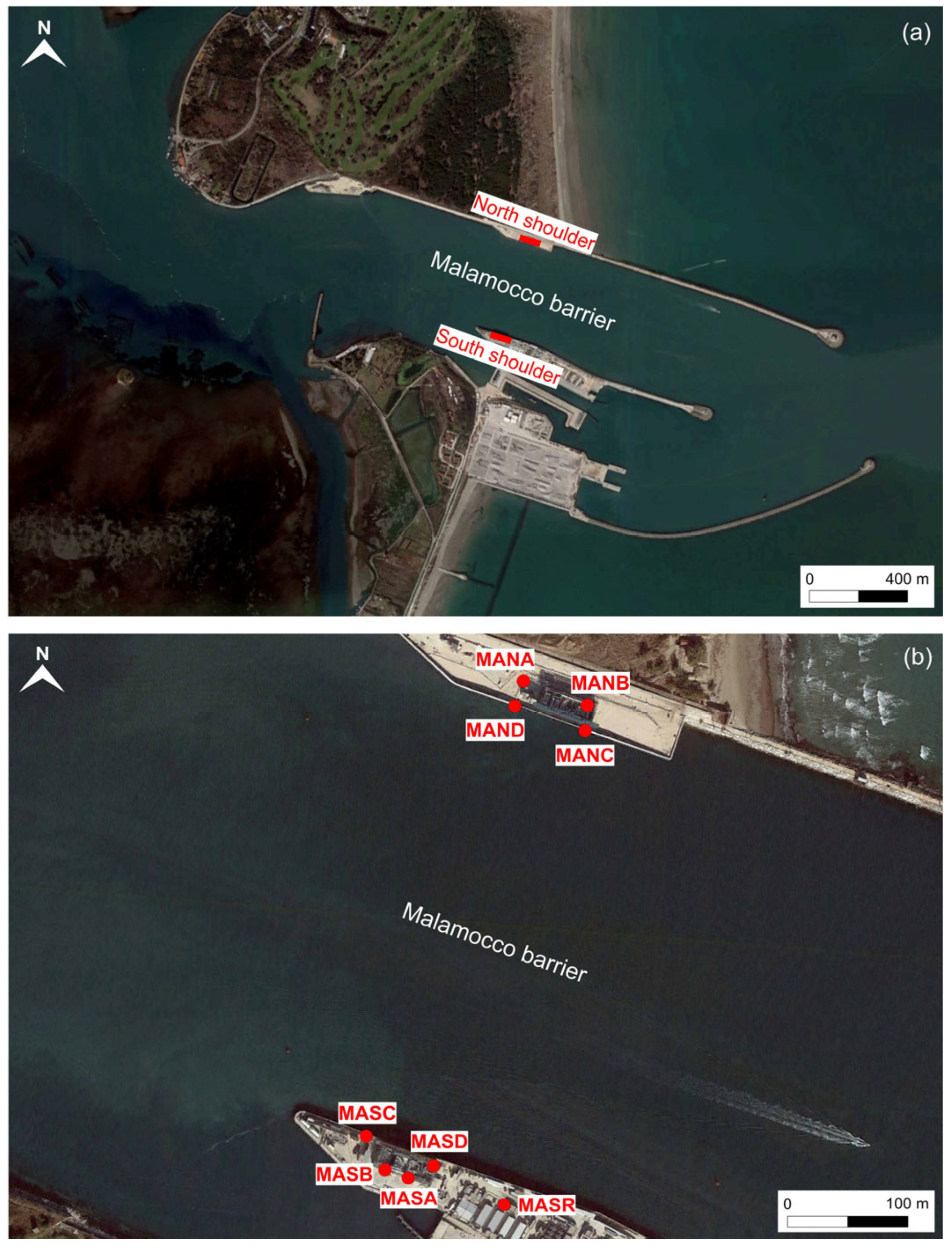
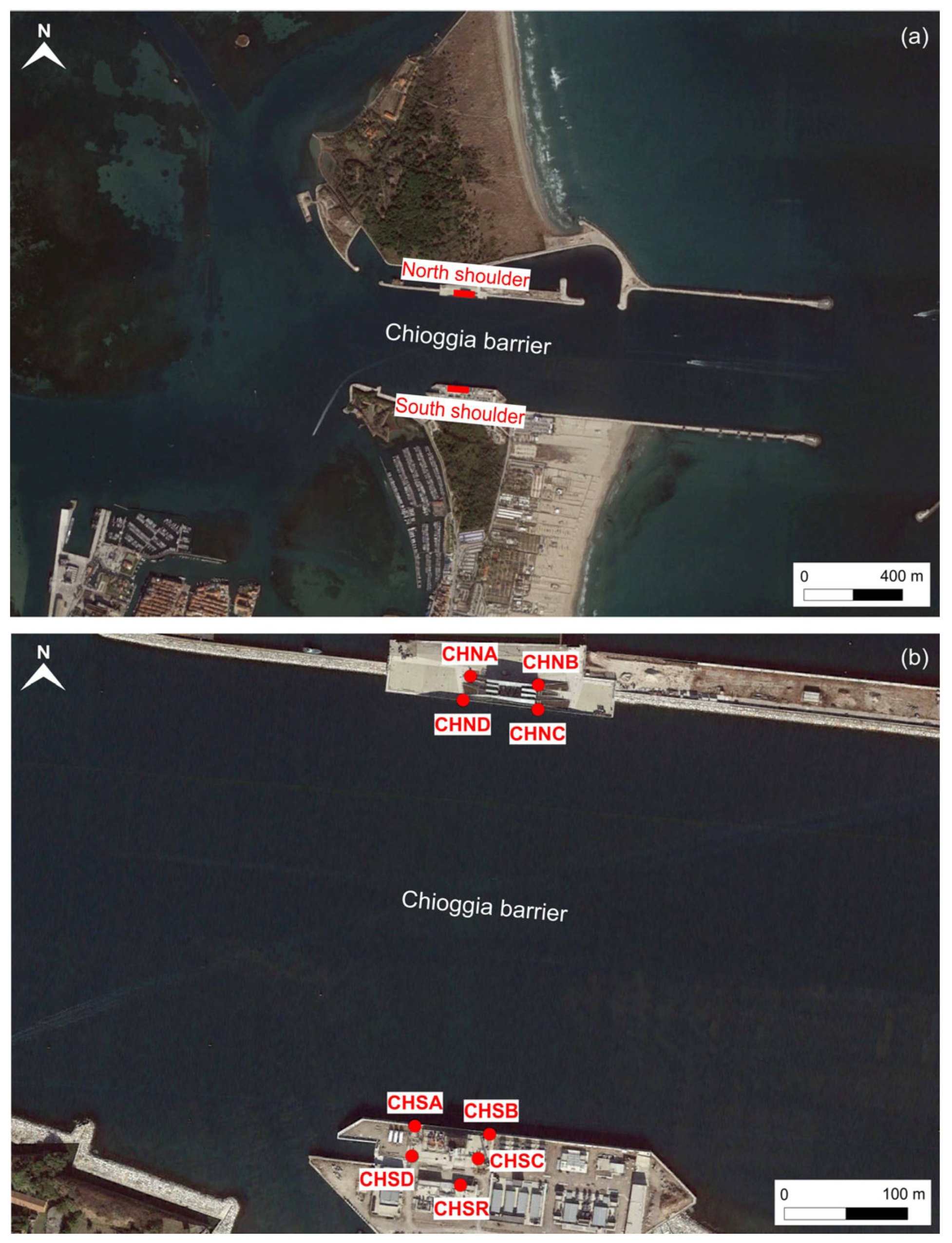
2.1. Overview of the MOSE System

The MOSE (MOdulo Sperimentale Elettromeccanico) system is an experimental electromechanical barrier designed to temporarily separate the city of Venice and its lagoon from the Adriatic Sea during severe storm surge events and high tides (Figure 1) [40]. The system, which is nearing completion, consists of four barriers located at the inlets of Treporti, San Nicolò, Malamocco, and Chioggia (Figure 1). At each barrier site, concrete lodging caissons were constructed and placed on the seabed, aligned longitudinally with the inlet [41] (Figure 3).
All caissons are fully submerged at depths ranging between 6 m and 20 m since each barrier has different morphological characteristics; only the two border caissons, known as the shoulder caissons, are provided with emerged structures (Figure 4). These last lateral caissons have dimensions of 16.7 m, 24 m, and 49.1 m (west caisson) and 16.7 m, 18.5 m, and 49.1 m (east caisson) in height, length, and width relative to the barrier, respectively (Treporti barrier). The caissons of each barrier are connected to each other by means of service tunnels, designed for maintenance activities, which can be reached using the stairwells from the emerged constructions of the shoulder caissons (for a better description of the system, see also [42]).
Typically, the system operates by raising the floodgates when the forecasted water level is higher than 110 cm. This safeguarding value was fixed based on the morphological characteristics of the city of Venice, as under these conditions, most of the pavements in the historic center become inundated [43]. However, to protect the city from flooding, the frequency of floodgate activation is expected to increase in the next years due to the effects connected to the rise of sea level [44], land subsidence [37,45], and coastal changes [46], that will significantly impact the upper Adriatic Sea.

2.2. CGNSS Observations and Processing Strategies

GNSS observations were derived from 36 continuous stations, nine for each of the Treporti, San Nicolò, Malamocco, and Chioggia barriers. The antennas were fixed close to the corners of the two shoulder structures on the basis of the available spaces and the most favorable conditions for the acquisition of the GNSS signal (e.g., maximizing the unobstructed horizon view and limiting as much as possible the multipath effects); in this way, the 3D monitoring of the shoulder caissons can be obtained assuming the non-deformability of the concrete objects. Furthermore, for each barrier, a reference station was located nearby, outside of the structures to be monitored (Figure 5, Figure 6, Figure 7 and Figure 8).
The 36 stations were installed between February 2021 and November 2022, using Trimble NET R9 receivers with Trimble Zephyr 3 Geodetic antennas for the stations on the emerged structures of the shoulder caissons, and Trimble Alloy receivers with Trimble Choke Ring antennas for the stations on the reference locations. Unfortunately, during the acquisition period, several works were carried out on the upper shoulder structures near the GNSS antennas, as the buildings were being completed. In particular, new masquerading was installed on top of the concrete elements, covering a significant portion of the visible sky. The consequences were the relocation of some stations (TREB, SNNA), where coverage issues and/or severely disturbed signals were identified.
Continuous GNSS stations were installed to generate an automatic deformation monitoring system of the MOSE infrastructure in each barrier. The 32 CGNSS stations of the shoulder caissons and other sensors located in the tunnels (eight strain gauges, 70 inclinometers, one for each caisson, and joints measuring devices fixed in the separation between the adjacent caissons) will be connected. Starting from the CGNSS data, the movements of the caissons will be automatically calculated following the sequence of installed sensors, with a chain that starts from the GNSS data of a shoulder caisson of the barrier, continues with the strain gauge, proceeds in the tunnels, rises in the opposite shoulder caisson, and closes in the GNSS data; in this way, the floodgate gaps and the rubber joints deformation monitoring will be automatically performed (for more details, see [42]).
In this work, the GNSS observations available from daily RINEX files (30 s sampling rates), acquired from the dates of installation up to 30 May 2023, were processed using Bernese version 5.4 software [47] to obtain the velocities of the CGNSS stations in the period analyzed. The coverage of the RINEX files was 71.64%, 94.74%, and 42.23% for 2021, 2022, and 2023, respectively. Data processing was carried out using the following three different strategies:
(i) Solving a network composed of the 36 permanent stations of the MOSE system together with eight external CGNSS reference stations located in the vicinity of the Venice Lagoon (Figure 1). TRVS, SDNA, VEN1, PADO, PORE, ROVI, TGPO, and GARI were chosen based on their geographical position, the availability of open data, and as belonging to the EUREF Permanent GNSS Network and the Italian rete dinamica nazionale (RDN) network (GNSS–1).
(ii) Solving a network composed of the same eight continuous external GNSS reference stations together with the reference stations of the four barriers (TRWR, SNNR, MASR, and CHSR). After the calculation of the positioning and velocities of the four reference stations of the MOSE system, the four sub-networks composed of the nine stations of each barrier were processed, fixing the position and velocity of the reference station previously calculated (GNSS–2).
In both strategies, data were aligned with the ITRF2014 reference frame; subsequently, removing the horizontal motion of the Eurasia plate, the ETRF2014 realization was obtained [48].
(iii) Further processing was performed using daily RINEX files from selected dates. In this approach, for each sub-network of the four barriers, the baselines were calculated using the Leica Infinity software version 4.0.0.44003, and the sub-network was adjusted to fix the reference CGNSS station. In this way, for each of the selected dates, the coordinates of the other CGNSS stations were calculated. Repeating this approach using the RINEX file from other dates, the new coordinates of the stations were obtained. Subsequently, by comparing the coordinates, the velocities were extracted. The dates of the RINEX files were chosen considering a time difference of approximately 3/4 months, based on the multi-temporal completeness of the data. The comparison was made between the coordinates related to the same dates of 2021, 2022, and 2023, to avoid seasonal deformations on the calculated velocities. In this analysis, GPS days of 150, 234, and 335 were selected for Treporti, 150, 234, and 357 for San Nicolò, 150 for Malamocco, and 70 for Chioggia barriers (GNSS–3).

2.3. InSAR Data

InSAR data used in this study were obtained from the European Ground Motion Service (EGMS) of the Copernicus program [49] and the Veneto Region Sentinel-1 PS database [50]. Both services provide open data related to the LOS velocities obtained from Advanced-DInSAR processing (i.e., PS-InSAR [51] and SqueeSAR [52]) of the SAR images acquired by Sentinel-1.
The EGMS service offers three levels of products: Basic, Calibrated, and Ortho [53]. In this study, the Calibrated products were considered. These consist of a dataset of points derived from interferometric analyses of Sentinel-1 images, as in the case of the Basic products, but referenced to a model derived from the European GNSS data network. The points have various attributes, including quality indices, estimated average velocity over the observation period (measured along the LOS), and displacement time series. The data provide spatial coverage that extends across the European Community and provide estimates of surface deformation rates with millimeter-level precision [54].
The Veneto Region service provides point datasets derived from interferometric analyses of Sentinel-1 data using the SqueeSAR technique. The datasets contain information on the annual average velocities of the ground targets and the displacement time series. The service covers the entire Veneto Region (northeastern Italy) and is aimed at civil protection purposes.
Table 1 reports the available InSAR data in detail. Note that EGMS InSAR data do not perfectly overlap with the CGNSS observations, since the GNSS observations cover five more months in 2023.

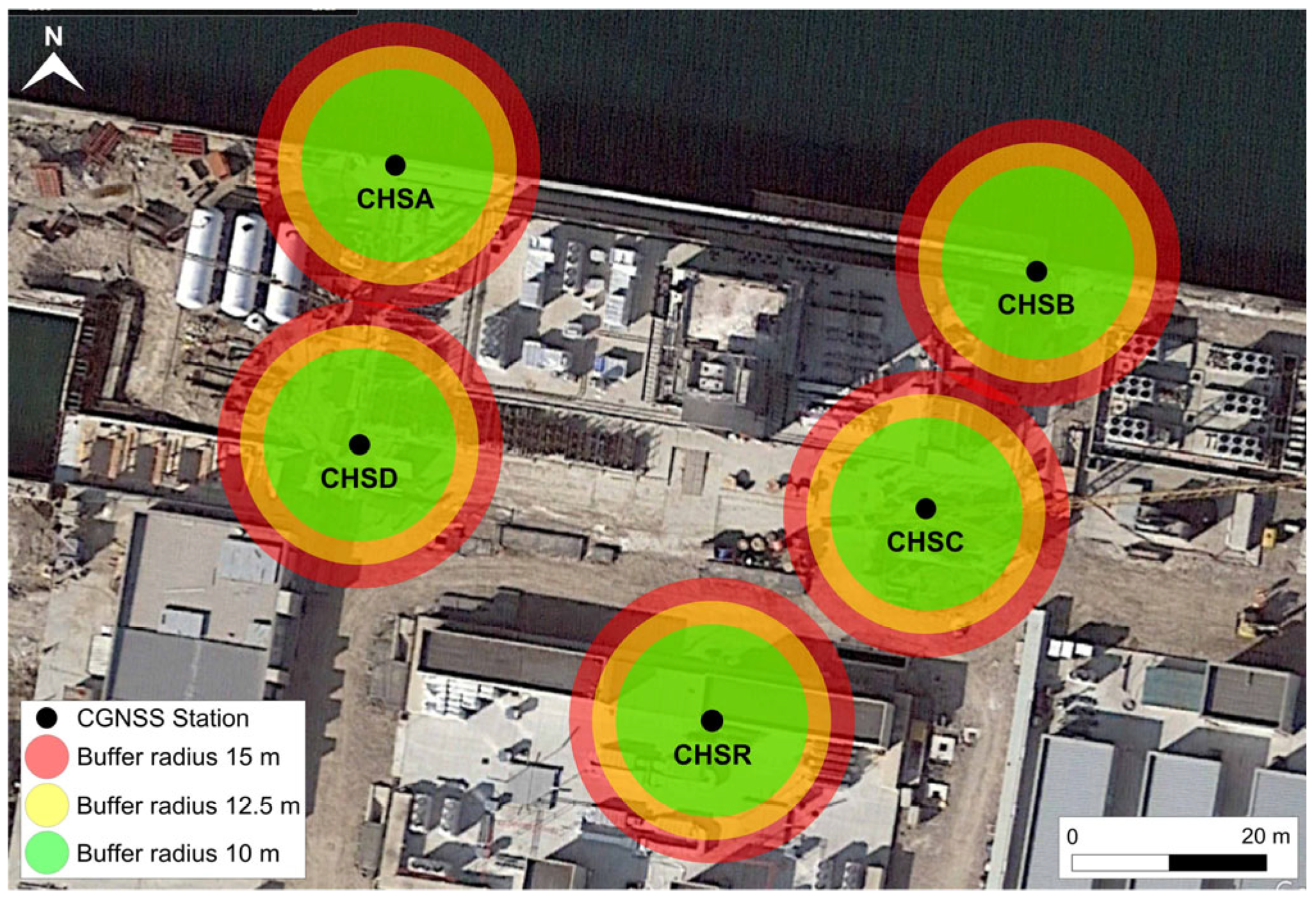
2.4. Calibration and Validation of Interferometric Data

InSAR velocities were compared with the CGNSS data to calibrate and validate the EGMS and Veneto Region interferometry products in the area of the MOSE system, considering ground-based CGNSS measurements to be more reliable. In the first phase, the satellite data were compared with the VEN1 CGNSS velocity, the closest to the MOSE barriers and external to the construction sites. If a difference was found between the velocities of the InSAR points and the CGNSS values, the interferometric data were calibrated. In the comparison procedure, InSAR points enclosed in a circle centered on the GNSS station and with a radius of 15 m were selected; their mean velocity was compared, and then calibrated, with the GNSS velocity of the analyzed station projected along the satellite LOS. The other CGNSS stations of the external network were used to validate the new interferometric velocities obtained. This phase of calibration and validation did not involve the continuous stations of the MOSE system, as the anthropic works near the GNSS antennas could generate artificial velocities in the InSAR image processing, making them noncomparable with those measured by the GNSS antennas. In the second phase, the described comparison approach was applied to the 36 CGNSS stations of the MOSE. In detail, the mean velocities of InSAR points located on shoulder structures, enclosed in a buffer zone centered on the GNSS stations with radii of 15 m, 12.5 m, and 10 m, were calculated (Figure 9). These values, obtained before and after calibration, were compared with those of the CGNSS stations, using the GNSS–1 and GNSS–2 solutions projected on the LOS. The definition of the three different radii was established to evaluate the changes in velocities based on the distance of the PSs from the CGNSS station. The radii values were chosen as a compromise between the need to: (i) identify PSs for comparisons; (ii) obtain points near the corners of the shoulder structures; and (iii) minimize significant overlap between buffers, thereby preventing the same PSs from being used in velocity analysis for different corners.

3. Results

3.1. GNSS Solutions

GNSS velocities were obtained for the 36 continuous stations of the MOSE system following the three strategies, GNSS–1, GNSS–2, and GNSS–3, described in Section 2.2. The results were strongly influenced by the temporal length and continuity of the time series. Moreover, due to ongoing anthropic works around the CGNSS stations and the installation of masquerading on the roofs of the shoulder caisson, the observations were influenced by the multipath phenomenon. The obtained north–south and east–west horizontal components of the velocities were very small (on the order of 1 mm/year) compared to the vertical contribution, as expected, as structures were essentially exhausted before the installation of GNSS antennas; a confirmation of this effect was also provided by the topographic data [42]. For this reason, only the vertical component has been analyzed. As an example of the obtained vertical velocities, Table 2 shows the values calculated using the three processing strategies in the Chioggia barrier, where the time series is of about 2 years, while for the CHNB station, it is limited to only 6 months.
When the analyzed time series of the CGNSS stations are very similar in terms of temporal coverage for all stations of the same barrier (time series observations of more than 2 years and without significant interruption of acquisitions), the GNSS–1 and GNSS–2 strategies provide comparable velocities. As an example, Table 3 shows the vertical velocities obtained using the three processing strategies in the Treporti barrier, the most completed in terms of CGNSS observations.

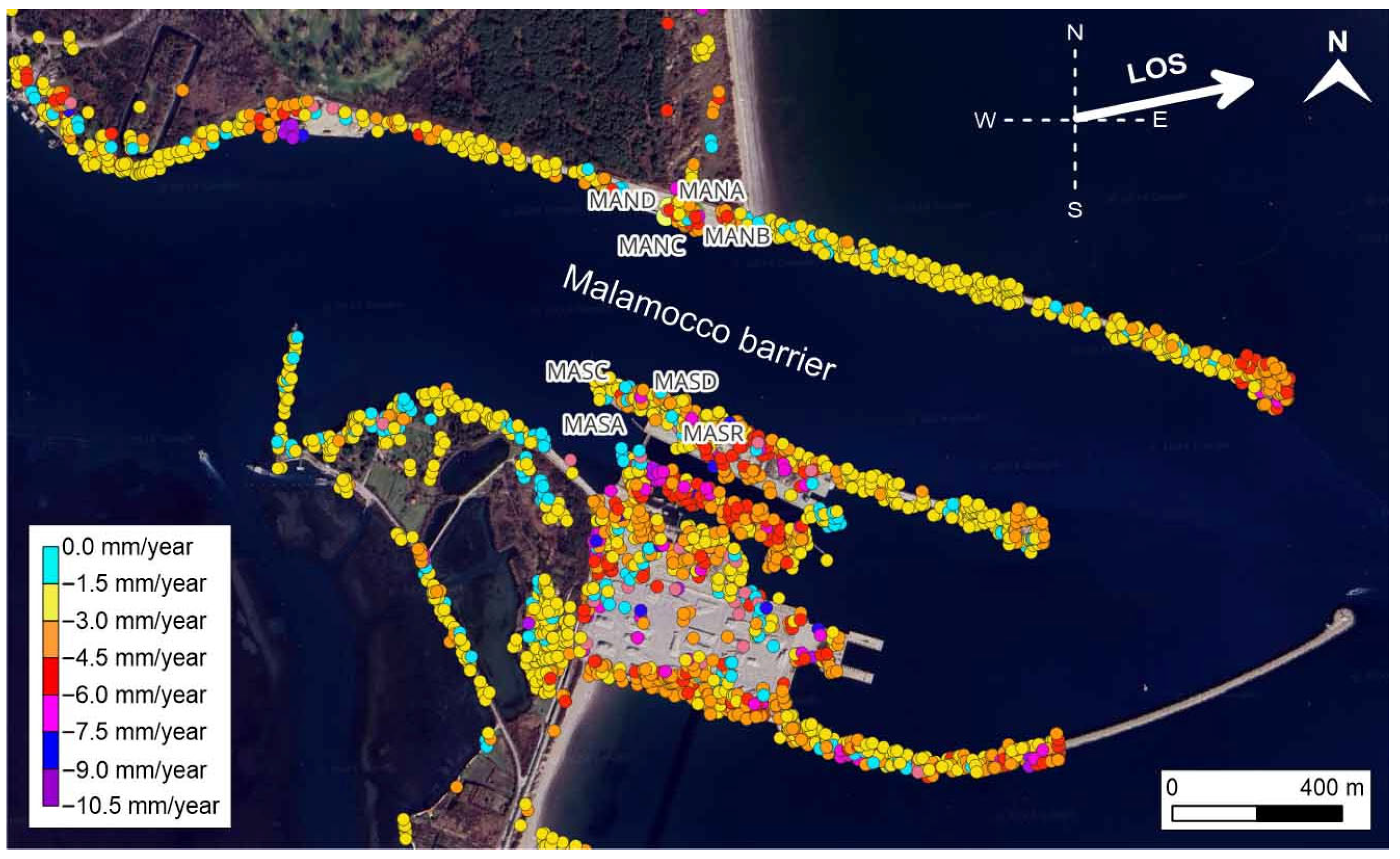
3.2. CGNSS–InSAR Velocities Comparison

In the first phase, a comparison was made to calibrate the EGMS and Veneto Region InSAR data using the VEN1 CGNSS station. The mean velocity of PSs up to 15 m from VEN1 was compared with the vertical velocity of the CGNSS station projected along the LOS of the satellite. In general, if a horizontal component of the GNSS velocity had been obtained, the comparison with the InSAR data would have been performed by combining the horizontal and vertical velocities projected along the LOS, using well-known geometric relations. In Table 4, the differences obtained before and after calibration, for the ascending tracks 44 and 117, and the descending track 95 of the EGMS dataset, are reported. The same values were calculated at the SDNA and PADO CGNSS stations, i.e., those available and used for validation.
The same approach applied to the Veneto Region dataset provided the results shown in Table 5.
In the second phase, the comparisons between velocities involved the 36 CGNSS stations of the MOSE system to evaluate the level of agreement between the two datasets at the construction sites. In this case, only PSs on shoulder structures and up to 15 m, 12.5 m, and 10 m from the CGNSS stations were analyzed. The mean values, before and after the calibration obtained from the first phase, were compared with the vertical velocity of the CGNSS stations projected along the LOS and obtained from both the GNSS–1 and the GNSS–2 solutions. Table 6 shows the calculated percentages of differences between velocities less than 1.5 mm/year for tracks 44, 117, and 95 of the EGMS dataset. In these comparisons, interferometric mean velocities obtained before and after calibration using the VEN1 station were used.
The same approach applied to the Veneto Region dataset provided the results shown in Table 7.

3.3. CGNSS–InSAR Data Integration

In the last phase, GNSS and InSAR data were integrated, extracting maps of velocities in the areas of the MOSE system. As an example, in Figure 10, Figure 11 and Figure 12, the velocities obtained using track 44 of the EGMS dataset and the GNSS–1 solution for the Treporti and San Nicolò, Malamocco, and Chioggia barriers are shown. The maximum deformations were on the order of 10 mm/year in the construction areas of the MOSE system, significantly different from those obtained by [55] during the initial construction phases and periods of intense anthropic activity. They applied Interferometric Point Target Analysis (IPTA) [56], a particular PSI chain, on 30 TerraSAR-X stripmap images and 31 COSMO-SkyMed stripmap images covering the period 2008–2011 and calibrated using permanent GPS stations. The authors provided velocities in the range of 10–25 mm/year and, in some cases, greater than 25 mm/year in the inlets of Lido, Malamocco, and Chioggia.

4. Discussion

The vertical velocities obtained from GNSS observations for the Chioggia and Treporti barriers are shown in Table 2 and Table 3, respectively. The values reported in Table 2 show similar velocities for the CGNSS stations located in the same shoulder caisson and obtained using the GNSS–1 and GNSS–2 strategies, excluding the CHNB station in the north shoulder caisson. Note that, while the time series for all the stations cover more than 2 years of observations, the dataset for CHNB is limited to only 6 months. Furthermore, the velocities obtained with the GNSS–1 and GNSS–2 strategies provided similar values for each station, since the differences are less than 0.8 mm/year. In contrast, different velocities were obtained using the GNSS–3 strategy, with differences—both between stations belonging to the same shoulder structure and between those derived from the GNSS–1 and GNSS–2 strategies—reaching values of up to 3.31 mm/year and 2.37 mm/year, respectively. For these reasons, the GNSS–3 processing strategy was considered unsuitable for this application. Averaging the velocities related to the CGNSS stations in the same shoulder caisson (excluding the CHNB station), the obtained values showed differences between the North and the South shoulder structures of the order of 0.5 mm/year, for both the GNSS–1 and GNSS–2 strategies. In this way, no significant differential displacement was detected between the lateral shoulder caissons of the Chioggia barrier.
The values reported in Table 3 for the Treporti barrier show similar velocities both for the CGNSS stations belonging to the same shoulder caisson (max differences less than 0.9 mm/year) and obtained with the GNSS–1 and GNSS–2 strategies (max differences less than 0.4 mm/year). The GNSS–3 strategy was confirmed to be inappropriate for this type of application. Moreover, similar differences were observed in the other barriers of the MOSE system, and for these reasons, the results of this strategy were not used hereafter. As in the Chioggia barrier, the GNSS–3 strategy provided significant differential velocities, both for the CGNSS stations belonging to the same shoulder caisson (max differences of up to 3.07 mm/year) and for those obtained with the GNSS–1 and GNSS–2 strategies (max differences of up to 3.03 mm/year). The average velocities between the stations located in the same shoulder caisson showed differences of 1.09 mm/year between the East and West structures considering the GNSS–1 strategy and a mitigated value of 0.72 mm/year using the GNSS–2 strategy. Even though the topographic data do not suggest differential movements between the shoulder caissons of the barrier, these values should be monitored as the time series increase.
The general considerations developed for the Chioggia and Treporti barriers can be extended to the San Nicolò and Malamocco ones. In particular, the problems described for the CHNB CGNSS station in the Chioggia barrier (overall linked to the temporal coverage of the time series) were detected for the SNNR station in San Nicolò, and the MASA and MASD stations in the Malamocco barriers. Additionally, significant multipath problems were detected for the MANC station during the analyzed period, suggesting a change of position to achieve better signal acquisition.
The level of agreement between GNSS and InSAR velocities was evaluated considering the percentages of differences less than a defined threshold value, representing the uncertainties when GNSS and InSAR velocities are analyzed, compared, and combined. The definition of this parameter is crucial. Some studies analyzed the quality of Sentinel-1 ground datasets and found evidence of achievable submillimeter accuracy for annual displacement rates [7]. Ng et al. [38] compared Sentinel-1 data with CGNSS velocities to evaluate the land subsidence in Sydney. The authors obtained mean differences of less than 1 mm/year and RMS differences of the order of 1 mm/year but with some differences greater than 2 mm/year. Huang et al. [57], investigating the structural safety assessment of high buildings in the Guangzhou–Foshan metropolitan area, compared the deformation velocity of 45 InSAR points with the GNSS deformation velocity of the continuous GUAN station, obtaining an overall RMSE of 1.50 mm/year, the same value suggested by [17]. In this study, due to the complexity of the MOSE system linked to signal disturbances, both for the GNSS observations and the interferometric data caused by continuous works, a realistic uncertainty threshold of 1.5 mm/year was adopted.
Based on the fixed threshold, Table 4 (EGMS dataset) shows that, although the calibration procedure worsens the difference at the SDNA validation station for track 44, the difference obtained after the correction remains less than the threshold velocity (1.5 mm/year). For track 117, there were no stations available for validation, but in this case, the correction is only −0.22 mm/year. An effective improvement was obtained for track 95 since at the PADO validation station, the difference after calibration is within the threshold value.
In the case of the Veneto Region dataset (Table 5) before calibration, five differences in velocities provided values greater than 1.5 mm/year (45%). Calibration using the VEN1 station improved the level of agreement between GNSS and InSAR velocities, since only two differences after the correction exceeded the threshold value of 1.5 mm/year (18%).
The analysis of Table 6 (percentages of differences between velocities lower than 1.5 mm/year–EGMS dataset) shows a decrease percentage of differences between velocities lower than 1.5 mm/year after calibration for track 44. However, the mean value before and after calibration is very similar (65% vs. 59%).
The results after calibration improve for tracks 117 and 95 (75% of the differences greater than 1.5 mm/year before calibration fall within the used threshold value after calibration), since the mean percentage of differences of velocities less than 1.5 mm/year after calibration increases significantly (from 62% to 72% for track 117 and from 49% to 67% for track 95).
The same approach was applied to the Veneto Region dataset (Table 7). In this case, a significant improvement of the results after calibration has been obtained, since the percentages increased in all comparisons: for track 117 (mean value from 42% before calibration to 73% after calibration) and track 95 (mean value from 29% before calibration to 68% after calibration).
The calibration improved the agreement between GNSS and InSAR velocities at the MOSE system construction sites for both the EGMS and Veneto Region datasets, except for track 44 (EGMS data). The agreement level was around 70% of the analyzed velocity differences, acknowledging that ongoing works near the GNSS antenna had a strong influence on this result.
Figure 10, Figure 11 and Figure 12, which show the velocities along the satellite LOS integrating the GNSS–1 solution with the InSAR EGMS dataset (track 44) for the MOSE construction sites and surrounding areas, highlight that the velocities obtained in this work confirm the general stability of the emerged structures, with most of the deformations gradually stabilizing. Furthermore, outside of the construction site areas, the velocities, in the order of 3–5 mm/year, agree with the values observed along the surrounding Venetian coast [37].

5. Conclusions

In this study, 36 CGNSS stations and InSAR data from the EGMS and Veneto Region interferometry services were used to monitor the deformation of the shoulder structures of the MOSE system, a strategic infrastructure designed to protect the Venice Lagoon, particularly the historic city center, from flooding.
CGNSS observations were processed using three strategies, along with eight CGNSS stations located around the Venice Lagoon as a reference external network. The first and second strategies, based on time series analysis, provided similar velocities, since the only difference was the configuration of the networks in the data processing. On the contrary, the third solution, based on comparisons of multitemporal daily positioning, provided unsuitable velocities for this study and was therefore excluded.
The available InSAR velocities were compared with the GNSS results to calibrate, validate, and integrate the interferometric data with ground-based GNSS measurements. After data calibration, the level of agreement between velocities in the MOSE system area was evaluated based on a defined threshold value of the differences. A value of 1.5 mm/year was set to determine the accuracy of the data. The comparison results showed that, before and after the calibration of the EGMS InSAR data, 59% and 66% of the differences, respectively, were below 1.5 mm/year on average. The same procedure applied to the Veneto Region InSAR dataset provided an average of 36% and 71% of differences lower than the threshold value before and after calibration, respectively.
The analysis of the GNSS velocities of the 36 continuous stations did not provide significant horizontal deformations of the shoulder caissons, while the vertical values were very close to the land subsidence trend of the study area. Furthermore, no significant differential velocities of the border shoulder caissons were detected, confirming the general stability of the emerging structures in all the barriers.
The interferometric calibrated velocities allowed one to extend the deformation monitoring to both the construction sites and surrounding areas. Maximum deformation of the order of 10 mm/year (mainly due to anthropic activities) and land subsidence trends were obtained for the construction sites and surrounding areas, respectively.
Finally, this work provides an opportunity to analyze open datasets that are very useful to researchers for studies of different phenomena. The increase in sensors on different platforms that acquire continuous data, linked to near-real-time automatic processing, is expected to increase in the next few years. The calibration, validation, and evaluation of the performance of these large datasets will pose a real challenge in the coming years.

Author Contributions

Conceptualization, M.F. (Massimo Fabris) and M.F. (Mario Floris); methodology, M.F. (Massimo Fabris) and M.F. (Mario Floris); software, M.F. (Massimo Fabris); validation, M.F. (Massimo Fabris) and M.F. (Mario Floris); formal analysis, M.F. (Massimo Fabris) and M.F. (Mario Floris); investigation, M.F. (Massimo Fabris) and M.F. (Mario Floris); resources, M.F. (Massimo Fabris) and M.F. (Mario Floris); data curation, M.F. (Massimo Fabris); writing—original draft preparation, M.F. (Massimo Fabris); writing—review and editing, M.F. (Massimo Fabris) and M.F. (Mario Floris); visualization, M.F. (Massimo Fabris) and M.F. (Mario Floris); supervision, M.F. (Massimo Fabris); project administration, M.F. (Massimo Fabris); funding acquisition, M.F. (Massimo Fabris) All authors have read and agreed to the published version of the manuscript.

Funding

This research received no external funding.

Data Availability Statement

Restrictions apply to the availability of the GNSS data. Data were obtained from Consorzio Venezia Nuova.

Acknowledgments

The authors would like to thank the “Ministero delle Infrastrutture e dei Trasporti—Provveditorato Interregionale per le Opere Pubbliche del Veneto—Trentino Alto AdigeFriuli Venezia Giulia”; Consorzio Venezia Nuova; Irene D’Urso, MSCE (Master of Science in Civil Engineering), and Massimo Pravato of Thetis SpA; the “Laboratory of Geomatics and Surveying” staff at the University of Padova.

Conflicts of Interest

The authors declare no conflicts of interest.

References

  1. Scaioni, M.; Marsella, M.; Crosetto, M.; Tornatore, V.; Wang, J. Geodetic and Remote-Sensing Sensors for Dam Deformation Monitoring. Sensors 2018, 18, 3682. [Google Scholar] [CrossRef] [PubMed]
  2. Cenni, N.; Fiaschi, S.; Fabris, M. Monitoring of Land Subsidence in the Po River Delta (Northern Italy) Using Geodetic Networks. Remote Sens. 2021, 13, 1488. [Google Scholar] [CrossRef]
  3. Cenni, N.; Mantovani, E.; Baldi, P.; Viti, M. Present kinematics of Central and Northern Italy from continuous GPS measurements. J. Geodyn. 2012, 58, 62–72. [Google Scholar] [CrossRef]
  4. Yuwono, B.D.; Prasetyo, Y. Analysis Deformation Monitoring Techniques Using GNSS Survey and Terrestrial Survey (Case Studi: Diponegoro University Dam, Semarang, Indonesia). IOP Conf. Ser. Earth Environ. Sci. 2018, 313, 012045. [Google Scholar] [CrossRef]
  5. Magnaval, G.; Colette, T.; Boumeshal, M. Combination of Total Station and GNSS for the Monitoring of Civil Infrastructures in Dense Urban Areas. Proocedings of the 10th European Workshop on Structural Health Monitoring, EWSHM, Palermo, Italy, 4–7 July 2022; Code 279319 Lecture Notes in Civil Engineering. Springer: Berlin/Heidelberg, Germany, 2023; Volume 254, pp. 51–58. [Google Scholar]
  6. Motagh, M.; Djamour, Y.; Walter, T.R.; Wetzel, H.-U.; Zschau, J.; Arabi, S. Land subsidence in Mashhad Valley, northeast Iran: Results from InSAR, levelling and GPS. Geophys. J. Int. 2007, 168, 518–526. [Google Scholar] [CrossRef]
  7. Cigna, F.; Ramírez, R.E.; Tapete, D. Accuracy of Sentinel-1 PSI and SBAS InSAR Displacement Velocities against GNSS and Geodetic Leveling Monitoring Data. Remote Sens. 2021, 13, 4800. [Google Scholar] [CrossRef]
  8. Wang, Q.; Gao, Y.; Gong, T.; Liu, T.; Sui, Z.; Fan, J.; Wang, Z. Dam Surface Deformation Monitoring and Analysis Based on PS-InSAR Technology: A Case Study of Xiaolangdi Reservoir Dam in China. Water 2023, 15, 3298. [Google Scholar] [CrossRef]
  9. Karami, E.; Alizadeh, N.; Farhadi, H.; Abdolazimi, H.; Maghsoudi, Y. Monitoring of land surface displacement based on SBAS-InSAR time-series and GIS techniques: A case study over the Shiraz Metropolis, Iran. ISPRS Ann. Photogramm. Remote Sens. Spat. Inf. Sci. 2023, X-4/W1-202, 371–378. [Google Scholar] [CrossRef]
  10. Xiao, R.; Gao, X.; Wang, X.; Yuan, S.; Wu, Z.; He, X. Measuring Dam Deformation of Long-Distance Water Transfer Using Multi-Temporal Synthetic Aperture Radar Interferometry: A Case Study in South-to-North Water Diversion Project, China. Remote Sens. 2024, 16, 365. [Google Scholar] [CrossRef]
  11. Chen, X.; Achilli, V.; Fabris, M.; Menin, A.; Monego, M.; Tessari, G.; Floris, M. Combining Sentinel-1 Interferometry and Ground-Based Geomatics Techniques for Monitoring Buildings Affected by Mass Movements. Remote Sens. 2021, 13, 452. [Google Scholar] [CrossRef]
  12. Alonso-Díaz, A.; Solla, M.; Rodríguez, J.L.; Elseicy, A. Integrated approach to improve Road Infrastructure Resilience through complementary Non-Destructive Techniques. In Proceedings of the 19th 3D GeoInfo Conference 2024—ISPRS Annals of the Photogrammetry, Remote Sensing and Spatial Information Sciences, Vigo, Spain, 1–3 July 2024; Volume X-4/W5-2024, pp. 9–15. [Google Scholar] [CrossRef]
  13. Casu, F.; Manzo, M.; Lanari, R. A quantitative assessment of the SBAS algorithm performance for surface deformation retrieval from DInSAR data. Remote Sens. Environ. 2006, 102, 195–210. [Google Scholar] [CrossRef]
  14. Qiu, D.; Wang, Y.; Zhang, Y.; Tong, Y.; Liang, H.; Ding, K.; Wan, S.; Wang, Y. Settlement monitoring data fusion approach for high-speed railways based on GNSS and InSAR. J. Appl. Remote Sens. 2023, 17, 034507. [Google Scholar] [CrossRef]
  15. Ellis, A.P.; Johanson, I.A.; Poland, M.P. Deformation of Mauna Loa before, during, and after its 2022 eruption. Bull. Volcanol. 2025, 87, 8. [Google Scholar] [CrossRef]
  16. Yeh, T.-K.; Lee, T.-Y.; Lee, I.-H.; Shih, H.-C.; Chen, C.-H.; Yen, J.-Y.; Ni, C.-F. Combination on GNSS precise point positioning and InSAR data fusion to monitor the land subsidence in Taiwan. Geomat. Nat. Hazards Risk 2025, 16, 2445632. [Google Scholar] [CrossRef]
  17. Fiaschi, S.; Fabris, M.; Floris, M.; Achilli, V. Estimation of land subsidence in deltaic areas through differential SAR interferometry: The Po River Delta case study (Northeast Italy). Int. J. Remote Sens. 2018, 39, 8724–8745. [Google Scholar] [CrossRef]
  18. Hu, X.; Lu, Z.; Pierson, T.C.; Kramer, R.; George, D.L. Combining InSAR and GPS to Determine Transient Movement and Thickness of a Seasonally Active Low-Gradient Translational Landslide. Geophys. Res. Lett. 2018, 45, 1453–1462. [Google Scholar] [CrossRef]
  19. Manunta, M.; De Luca, C.; Zinno, I.; Casu, F.; Manzo, M.; Bonano, M.; Fusco, A.; Pepe, A.; Onorato, G.; Berardino, P.; et al. The Parallel SBAS Approach for Sentinel-1 Interferometric Wide Swath Deformation Time-Series Generation: Algorithm Description and Products Quality Assessment. IEEE Trans. Geosci. Remote Sens. 2019, 57, 6259–6281. [Google Scholar] [CrossRef]
  20. Cigna, F.; Tapete, D. Present-day land subsidence rates, surface faulting hazard and risk in Mexico City with 2014–2020 Sentinel-1 IW InSAR. Remote Sens. Environ. 2021, 253, 1–19. [Google Scholar] [CrossRef]
  21. Beattie, A.; Ahmed, M.; Chu, T.; Gebremichael, E.; Elshalkany, M.; Abdelrehim, R. Temporal gravimetry, campaign and permanent GNSS, and interferometric radar techniques: A comparative approach to quantifying land deformation rates in coastal Texas. Sci. Total Environ. 2024, 956, 177280. [Google Scholar] [CrossRef]
  22. Zhu, M.; Liu, H.; Miao, C.; Li, G.; Zhang, Y.; Zhou, Y.; Cai, J.; Yang, S.; Wang, Y.; Wang, Y.; et al. Safety assessment of the Qinghai–Tibet railway: Monitoring, analysis, and prediction. Cold Reg. Sci. Technol. 2025, 231, 104395. [Google Scholar] [CrossRef]
  23. Magnússon, E.; Björnsson, H.; Rott, H.; Roberts, M.J.; Pálsson, F.; Guđmundsson, S.; Bennett, R.A.; Geirsson, H.; Sturkell, E. Localized uplift of Vatnajökull, Iceland: Subglacial water accumulation deduced from InSAR and GPS observations. J. Glaciol. 2011, 57, 475–484. [Google Scholar] [CrossRef]
  24. Cheng, S.; Perissin, D.; Lin, H.; Chen, F. Atmospheric delay analysis from GPS meteorology and InSAR APS. J. Atmos. Sol.-Terr. Phys. 2012, 86, 71–82. [Google Scholar] [CrossRef]
  25. Chen, B.; Deng, K.; Fan, H.; Yu, Y. Combining SAR interferometric phase and intensity information for monitoring of large gradient deformation in coal mining area. Eur. J. Remote Sens. 2015, 48, 701–717. [Google Scholar] [CrossRef]
  26. Tapete, D.; Morelli, S.; Fanti, R.; Casagli, N. Localising deformation along the elevation of linear structures: An experiment with space-borne InSAR and RTK GPS on the Roman Aqueducts in Rome, Italy. Appl. Geogr. 2015, 58, 65–83. [Google Scholar] [CrossRef]
  27. Saleh, M.; Becker, M. New estimation of Nile Delta subsidence rates from InSAR and GPS analysis. Environ. Earth Sci. 2018, 78, 6. [Google Scholar] [CrossRef]
  28. Farolfi, G.; Bianchini, S.; Casagli, N. Integration of GNSS and satellite InSAR data: Derivation of fine-scale vertical surface motion maps of Po Plain, Northern Apennines, and Southern Alps, Italy. IEEE Trans. Geosci. Remote Sens. 2019, 57, 319–328. [Google Scholar] [CrossRef]
  29. Grgić, M.; Bender, J.; Bašić, T. Estimating Vertical Land Motion from Remote Sensing and In-Situ Observations in the Dubrovnik Area (Croatia): A Multi-Method Case Study. Remote Sens. 2020, 12, 3543. [Google Scholar] [CrossRef]
  30. Gudmundsson, M.T.; Jónsdóttir, K.; Hooper, A.; Holohan, E.P.; Halldórsson, S.A.; Ófeigsson, B.G.; Cesca, S.; Vogfjörd, K.S.; Sigmundsson, F.; Högnadóttir, T.; et al. Gradual caldera collapse at Bárdarbunga volcano, Iceland, regulated by lateral magma outflow. Science 2016, 353, aaf8988. [Google Scholar] [CrossRef]
  31. Wilkinson, M.W.; McCaffrey, K.J.W.; Jones, R.R.; Roberts, G.P.; Holdsworth, R.E.; Gregory, L.C.; Walters, R.J.; Wedmore, L.; Goodall, H.; Iezzi, F. Near-field fault slip of the 2016 Vettore Mw 6.6 earthquake (Central Italy) measured using low-cost GNSS. Sci. Rep. 2017, 7, 4612. [Google Scholar] [CrossRef]
  32. Yaragunda, V.R.; Oikonomou, E. Monitoring the Los (Line of Sight) Deformation of the Corinth Canal, Greece Using SBAS and GNSS Techniques. In Proceedings of the IEEE International Geoscience and Remote Sensing Symposium (IGARSS 2024), Athens, Greece, 7–12 July 2024; pp. 11056–11061. [Google Scholar] [CrossRef]
  33. Deng, F.; Zumberge, M. Seafloor motion from offshore man-made structures using satellite radar images—A case study in the Adriatic Sea. Remote Sens. Environ. 2025, 318, 114543. [Google Scholar] [CrossRef]
  34. Maltese, A.; Pipitone, C.; Dardanelli, G.; Capodici, F.; Muller, J.-P. Toward a Comprehensive Dam Monitoring: On-Site and Remote-Retrieved Forcing Factors and Resulting Displacements (GNSS and PS–InSAR). Remote Sens. 2021, 13, 1543. [Google Scholar] [CrossRef]
  35. Nahli, A.; Simonetto, E.; Tatin, M.; Durand, S.; Morel, L.; Lamour, V. On the Combination of Psinsar and Gnss Techniques for Long-Term Bridge Monitoring. In Proceedings of the International Archives of the Photogrammetry, Remote Sensing and Spatial Information Sciences, XXIV ISPRS Congress (2020 edition), Nice, France, 31 August–2 September 2020; Volume XLIII-B3-2020, pp. 325–332. [Google Scholar] [CrossRef]
  36. Selvakumaran, S.; Rossi, C.; Marinoni, A.; Webb, G.; Bennetts, J.; Barton, E.; Plank, S.; Middleton, C. Combined InSAR and Terrestrial Structural Monitoring of Bridges. IEEE Trans. Geosci. Remote Sens. 2020, 58, 7141–7153. [Google Scholar] [CrossRef]
  37. Fabris, M.; Battaglia, M.; Chen, X.; Menin, A.; Monego, M.; Floris, M. An Integrated InSAR and GNSS Approach to Monitor Land Subsidence in the Po River Delta (Italy). Remote Sens. 2022, 14, 5578. [Google Scholar] [CrossRef]
  38. Ng, A.H.-M.; Liu, Z.; Du, Z.; Huang, H.; Wang, H.; Ge, L. A novel framework for combining polarimetric Sentinel-1 InSAR time series in subsidence monitoring—A case study of Sydney. Remote Sens. Environ. 2023, 295, 113694. [Google Scholar] [CrossRef]
  39. Roque, D.; Nuno Lima, J.; Perissin, D.; Paula Falcão, A.; Lemos, J.V.; Fonseca, A.M. Integrated InSAR and GNSS Monitoring Subsystem for an Arch Dam and Reservoir Banks. J. Surv. Eng. 2021, 147, 3. [Google Scholar] [CrossRef]
  40. Tomasicchio, G.R.; Salvadori, G.; Lusito, L.; Francone, A.; Saponieri, A.; Leone, E.; De Bartolo, S. A Statistical Analysis of the Occurrences of Critical Waves and Water Levels for the Management of the Operativity of the MoSE System in the Venice Lagoon. Stoch. Environ. Res. Risk Assess. 2022, 36, 2549–2560. [Google Scholar] [CrossRef]
  41. Casasso, A.; Di Molfetta, A.; Sethi, R. Groundwater monitoring at a building site of the tidal flood protection system ‘‘MOSE’’ in the Lagoon of Venice, Italy. Environ. Earth Sci. 2015, 73, 2397–2408. [Google Scholar] [CrossRef]
  42. Fabris, M.; Monego, M. A Drone-Based Structure from Motion Survey, Topographic Data, and Terrestrial Laser Scanning Acquisitions for the Floodgate Gaps Deformation Monitoring of the Modulo Sperimentale Elettromeccanico System (Venice, Italy). Drones 2024, 8, 598. [Google Scholar] [CrossRef]
  43. Umgiesser, G. The impact of operating the mobile barriers in Venice (MOSE) under climate change. J. Nat. Conserv. 2020, 54, 125783. [Google Scholar] [CrossRef]
  44. Antonioli, F.; Anzidei, M.; Amorosi, A.; Lo Presti, V.; Mastronuzzi, G.; Deiana, G.; De Falco, G.; Fontana, A.; Fontolan, G.; Lisco, S.; et al. Sea-level rise and potential drowning of the Italian coastal plains: Flooding risk scenarios for 2100. Quat. Sci. Rev. 2017, 158, 29–43. [Google Scholar] [CrossRef]
  45. Tosi, L.; Da Lio, C.; Strozzi, T.; Teatini, P. Combining L-and X-band SAR interferometry to assess ground displacements in heterogeneous coastal environments: The Po River Delta and Venice Lagoon, Italy. Remote Sens. 2016, 8, 308. [Google Scholar] [CrossRef]
  46. Fabris, M. Monitoring the Coastal Changes of the Po River Delta (Northern Italy) since 1911 Using Archival Cartography, Multi-Temporal Aerial Photogrammetry and LiDAR Data: Implications for Coastline Changes in 2100 A.D. Remote Sens. 2021, 13, 529. [Google Scholar] [CrossRef]
  47. Dach, R.; Lutz, S.; Walser, P.; Fridez, P. User Manual. In Bernese GNSS Software Version 5.2; Astronomical Institute, University of Bern, Bern Open Publishing: Bern, Switzerland, 2015. [Google Scholar]
  48. Altamimi, Z.; Rebischung, P.; Métivier, L.; Collilieux, X. ITRF2014: A new release of the International Terrestrial Reference Frame modeling nonlinear station motions. J. Geophys. Res. Solid Earth 2016, 121, 6109–6131. [Google Scholar] [CrossRef]
  49. European Ground Motion Service, EGMS. Available online: https://egms.land.copernicus.eu/ (accessed on 10 February 2025).
  50. Veneto Region. Available online: https://idt2.regione.veneto.it/portfolio/webgis-dei-dati-sentinel-1-ps/ (accessed on 25 July 2024).
  51. Ferretti, A.; Prati, C.; Rocca, F. Permanent scatterers in SAR interferometry. IEEE Trans. Geosci. Remote Sens. 2001, 39, 8–20. [Google Scholar] [CrossRef]
  52. Ferretti, A.; Fumagalli, A.; Novali, F.; Prati, C.; Rocca, F.; Rucci, A. A New Algorithm for Processing Interferometric Data-Stacks: SqueeSAR. IEEE Trans. Geosci. Remote Sens. 2011, 49, 3460–3470. [Google Scholar] [CrossRef]
  53. Crosetto, M.; Solari, L.; Balasis-Levinsen, J.; Bateson, L.; Casagli, N.; Frei, M.; Oyen, A.; Moldestad, D.A.; Mróz, M. Deformation monitoring at European scale: The copernicus ground motion service. Int. Arch. Photogramm. Remote Sens. Spatial Inf. Sci. 2021, XLIII-B3-2021, 141–146. [Google Scholar] [CrossRef]
  54. Crosetto, M.; Crippa, B.; Mróz, M.; Cuevas-González, M.; Shahbazi, S. Applications based on EGMS products: A review. Remote Sens. Appl. Soc. Environ. 2025, 37, 101452. [Google Scholar] [CrossRef]
  55. Tosi, L.; Strozzi, T.; Teatini, P. Cosmo-skymed versus TerraSAR-X -based interferometry for monitoring the mose settlements at the Venice lagoon inlets. In Proceedings of the IEEE International Geoscience and Remote Sensing Symposium (IGARSS), Munich, Germany, 22–27 July 2012; pp. 2837–2840. [Google Scholar] [CrossRef]
  56. Werner, C.; Wegmuller, U.; Strozzi, T.; Wiesmann, A. Interferometric point target analysis for deformation mapping. In Proceedings of the IEEE International Geoscience and Remote Sensing Symposium (IGARSS), Toulouse, France, 21–25 July 2003. [Google Scholar]
  57. Huang, D.; Qi, Z.; Lin, S.; Gu, Y.; Song, W.; Lv, Q. Investigating the Structural Health of High-Rise Buildings and Its Influencing Factors Using Sentinel-1 Synthetic Aperture Radar Imagery: A Case Study of the Guangzhou–Foshan Metropolitan Area. Buildings 2024, 14, 4074. [Google Scholar] [CrossRef]
Figure 1. Location of the study area (a); the eight CGNSS stations of the external GNSS network—TRVS (Treviso), SDNA (San Donà), VEN1 (Venezia), PADO (Padova), PORE (Porec), ROVI (Rovigo), TGPO (Taglio di Po), and GARI (Porto Garibaldi)—along with the four inlets of Treporti, San Nicolò, Malamocco, and Chioggia (b).
Remotesensing 17 01059 g001
Figure 2. The flowchart of this work.
Remotesensing 17 01059 g002
Figure 3. Scheme representing the characteristics of the concrete caissons and the yellow floodgates housed in them (a); the service tunnels for maintenance activities are also shown. The caissons were located on the seabed, longitudinally to the inlet of each barrier. The floodgates are raised during high tides and severe storm surges (b).
Remotesensing 17 01059 g003
Figure 4. Scheme representing a vertical section (a) and a plan (b) of the tunnels that connect the different concrete caissons. The caissons are submerged (in cyan); only the shoulder caissons are provided by emerged structures (in gray). The embedded floodgates are also represented (in yellow) (see also [42]).
Remotesensing 17 01059 g004
Figure 5. (a) Location of the shoulder structures (red rectangles) in the Treporti and San Nicolò barriers (Figure 1) separated by an artificial island; (b,c) show the location of the CGNSS stations closed to the corners of the caissons with the reference ones (red circles). The yellow rectangle (A) in (b) shows the area displayed in detail in Figure 5.
Remotesensing 17 01059 g005
Figure 6. Detail A of Figure 4b. The location of the CGNSS stations, TREA, TREB, TREC, and TRED, at the corners of the east shoulder caisson in the Treporti barrier are shown, together with images representing the Trimble Zephyr 3 geodetic antennas fixed on the emerged structures.
Remotesensing 17 01059 g006
Figure 7. (a) Location of the shoulder structures (red rectangles) in the Malamocco barrier (Figure 1); (b) location of the CGNSS stations close to the corners of the caissons, along with the reference station (red circles).
Remotesensing 17 01059 g007
Figure 8. (a) Location of the shoulder structures (red rectangles) in the Chioggia barrier (Figure 1); (b) location of the CGNSS stations close to the corners of the caissons, along with the reference station (red circles).
Remotesensing 17 01059 g008
Figure 9. Procedure for the comparison between the CGNSS and InSAR velocities in the Chioggia barrier (south shoulder, see Figure 7). InSAR points located on shoulder structures and enclosed in circles centered on the CGNSS station, with radii of 15 m, 12.5 m, and 10 m, were selected. For each group of points, the velocities were averaged and compared with the CGNSS one (obtained from both GNSS–1 and GNSS–2 solutions) projected along the satellite LOS.
Remotesensing 17 01059 g009
Figure 10. Map of velocities along the satellite LOS that integrates the GNSS–1 solution with the InSAR EGMS dataset (track 44) in the Treporti and San Nicolò barriers.
Remotesensing 17 01059 g010
Figure 11. Map of velocities along the satellite LOS that integrates the GNSS–1 solution with the InSAR EGMS dataset (track 44) in the Malamocco barrier.
Remotesensing 17 01059 g011
Figure 12. Map of velocities along the satellite LOS that integrates the GNSS–1 solution with the InSAR EGMS dataset (track 44) in the Chioggia barrier.
Remotesensing 17 01059 g012
Table 1. Main characteristics of the InSAR data used in this study.
DatasetOrbitTrackScenePeriod
EGMSAscending44267–268–269 03.02.2021–25.12.2022
Ascending117265–266–267 02.02.2021–30.12.2022
Descending95804–805–806 01.02.2021–29.12.2022
Veneto RegionAscending117Regional area02.02.2021–04.06.2023
Descending95Regional area01.02.2021–03.06.2023
Table 2. Velocities of the CGNSS stations in the Chioggia barrier using the 3 different processing strategies. The mean values related to the structures of the North and South shoulder are also reported.
Velocity of the CGNSS Stations (mm/Year)
StrategyCHNACHNBCHNCCHNDCHSACHSBCHSCCHSDCHSR
GNSS–1 −3.81−5.89−3.63−4.11−3.58−3.26−3.28−3.47−3.53
GNSS–2−3.46−5.03−2.88−3.63−2.91−2.57−3.05−3.39−3.20
Difference−0.35−0.86−0.75−0.48−0.67−0.69−0.23−0.08−0.33
GNSS–3−5.83−3.63−2.91−4.89−3.82−4.64−4.53−1.33−3.53
Mean velocity of the north shoulder caissonMean velocity of the south shoulder caisson
GNSS–1−3.85 1−3.40
GNSS–2−3.32 1−2.98
1 Excluding CHNB station.
Table 3. Velocities of the CGNSS stations in the Treporti barrier using the 3 different processing strategies. The mean values related to the East and West shoulder structures are also reported.
Velocity of the CGNSS Stations (mm/Year)
StrategyTREATREBTRECTREDTRWATRWBTRWCTRWDTRWR
GNSS–1 −3.19−3.83−2.99−3.63−4.04−4.70−4.50−4.77−5.99
GNSS–2−3.58−3.68−3.33−3.55−3.96−4.50−4.16−4.49−5.65
Difference0.39−0.150.34−0.08−0.08−0.20−0.34−0.28−0.34
GNSS–3−2.70−2.44−2.31−1.59−1.01−4.08−2.49−1.97−5.99
Mean velocity of the east shoulder caissonMean velocity of the west shoulder caisson
GNSS–1−3.41−4.50
GNSS–2−3.54−4.28
Table 4. Differences in velocities between the mean values of PSs with a maximum distance of 15 m from VEN1, SDNA, and PADO, and the vertical ones of the CGNSS stations projected on the LOS for tracks 44, 117, and 95 (EGMS dataset). The values obtained after calibration using the VEN1 station as a reference are also reported. BC: before calibration; AC: after calibration.
Differences Between Velocities (CGNSS–InSAR) on LOS (mm/Year)
TrackCalibrationStation of Calibration–VEN1Station of Validation
44BC1.08−0.37 (SDNA)
AC0−1.45 (SDNA)
117BC0.22
AC0
95BC0.722.13 (PADO)
AC01.41 (PADO)
Table 5. Differences in velocities between the mean values of PSs with a maximum distance of 15 m from PADO, ROVI, SDNA, TGPO, TRVS, and VEN1, and the vertical values of CGNSS stations projected on the LOS for tracks 117 and 95 (Veneto Region dataset). The values obtained after calibration using the VEN1 station as a reference are also reported. BC: before calibration; AC: after calibration.
Differences Between Velocities (CGNSS–InSAR) on LOS (mm/Year)
TrackCalibrationPADOROVISDNATGPOTRVSVEN1
117BC−0.54−1.03−1.542.320.12−0.82
AC0.29−0.21−0.713.140.940
95BC0.35−0.57−1.76−2.64−1.98
AC2.341.410.22−0.660
Table 6. Percentages of differences between velocities lower than 1.5 mm/year, obtained by comparing the average values of tracks 44, 117, and 95 (EGMS dataset). The comparison considers PSs points up to 15 m, 12.5 m, and 10 m from each CGNSS MOSE station, with vertical values calculated from the GNSS–1 and GNSS–2 solutions projected along the LOS. In these comparisons, interferometric mean velocities obtained before and after calibration using the VEN1 station were considered. The number of identified MOSE stations is reported in parentheses. BC: before calibration; AC: after calibration.
Percentage of Differences Between Velocities Less Than 1.5 mm/Year (Number of Identified MOSE Stations)
TrackSceneCalibrationGNSS–1 GNSS–2
Buffer 15 mBuffer 12.5 mBuffer 10 mBuffer 15 mBuffer 12.5 mBuffer 10 m
44267BC57 (7)60 (5)50 (4)43 (7)60 (5)50 (4)
AC43 (7)40 (5)50 (4)57 (7)60 (5)50 (4)
268BC81 (26)75 (24)74 (23)77 (26)58 (24)57 (23)
AC62 (26)63 (24)57 (23)73 (26)75 (24)65 (23)
269BC87 (15)72 (14)69 (13)67 (15)64 (14)62 (13)
AC67 (15)57 (14)38 (13)87 (15)64 (14)46 (13)
117266BC73 (15)67 (15)92 (12)47 (15)53 (15)58 (12)
AC79 (15)80 (15)92 (12)67 (15)53 (15)75 (12)
267BC64 (28)61 (23)67 (18)54 (28)57 (23)50 (18)
AC71 (28)65 (23)67 (18)67 (28)70 (23)78 (18)
95805BC42 (26)48 (23)43 (21)39 (26)44 (23)43 (21)
AC54 (26)70 (23)62 (21)58 (26)70 (23)67 (21)
806BC50 (4)50 (4)67 (3)50 (4)50 (4)67 (3)
AF75 (4)75 (4)100 (3)50 (4)50 (4)67 (3)
Table 7. Percentages of differences between velocities lower than 1.5 mm/year, obtained by comparing the average values of tracks 117 and 95 (Veneto Region dataset). The comparison considers PSs points up to 15 m, 12.5 m, and 10 m from each CGNSS MOSE station, with vertical values calculated from the GNSS–1 and GNSS–2 solutions projected along the LOS. In these comparisons, interferometric mean velocities obtained before and after calibration using the VEN1 station were considered. The number of identified MOSE stations is reported in parentheses. BC: before calibration; AC: after calibration.
Percentage of Differences Between Velocities Less Than 1.5 mm/Year (Number of Identified MOSE Stations)
TrackCalibrationGNSS–1 GNSS–2
Buffer 15 mBuffer 12.5 mBuffer 10 mBuffer 15 mBuffer 12.5 mBuffer 10 m
117BC38 (13)43 (7)20 (5)54 (13)57 (7)40 (5)
AC69 (13)57 (7)40 (5)85 (13)86 (7)100 (5)
95BC25 (16)23 (13)13 (8)31 (16)31 (13)50 (8)
AF63 (16)62 (13)88 (8)56 (16)62 (13)75 (8)
Disclaimer/Publisher’s Note: The statements, opinions and data contained in all publications are solely those of the individual author(s) and contributor(s) and not of MDPI and/or the editor(s). MDPI and/or the editor(s) disclaim responsibility for any injury to people or property resulting from any ideas, methods, instructions or products referred to in the content.

