Enhancing the Communication Bandwidth of FH-MIMO DFRC Systems Through Constellation Rotation Modulation

Abstract

This paper presents a technique based on Constellation Rotation Modulation (CRM) to enhance the communication bandwidth of Frequency-Hopping Multiple-Input Multiple-Output Dual-Function Radar and Communication (FH-MIMO DFRC) systems. The technique introduces the dimension of constellation diagram rotation without increasing the system bandwidth or power consumption, significantly improving communication efficiency. Specifically, CRM, by rotating the constellation diagram, combines with traditional Frequency-Hopping Code Selection (FHCS) and Quadrature Amplitude Modulation (QAM) to achieve higher data transmission rates. Through theoretical analysis and experimental verification, we demonstrate the specific modulation and demodulation principles of CRM, and we compare the differences between the minimum Euclidean distance-based and constellation diagram folding projection fast demodulation methods. The impact of the proposed modulation on radar detection range and detection performance was analyzed in conjunction with radar equations and ambiguity functions. Finally, achieved through simulation analysis of radar and communication systems, as well as actual system testing on an SDR platform, the simulation and experimental results indicate that CRM modulation can significantly enhance communication bandwidth while maintaining radar detection performance, thereby validating the accuracy and reliability of the theory.

1. Introduction

As wireless communication and radar detection technologies continue to advance, the demand for spectrum resources is rapidly increasing, driven by emerging applications such as 6G communication, low-altitude economy, smart transportation, and indoor positioning [1,2,3]. The scarcity of available spectrum has become a significant bottleneck. To make more efficient use of the limited spectrum, Dual-Function Radar and Communication (DFRC) systems have been proposed [4,5], which integrate communication and radar sensing by sharing hardware and signal processing components. This integration reduces system costs, size, and weight, while enhancing spectrum efficiency and improving performance in both radar and communication functionalities [6].

At present, Frequency-Hopping Multiple-Input Multiple-Output (FH-MIMO) DFRC architectures have garnered significant attention [7]. To enhance communication symbol transmission rates, MIMO radars offer a high degree of freedom (DoF) in waveform design, allowing for the optimization of beam patterns. This capability enables the embedding of communication information into sidelobes through modulation schemes such as Phase Shift Keying (PSK) and Amplitude Shift Keying (ASK) [8,9]. Furthermore, non-traditional modulation techniques, such as Code Shift Keying (CSK) [10] and waveform shuffling [11], have been applied to MIMO radar waveforms, allowing for increased data transmission per symbol. However, these techniques are typically constrained by the radar’s pulse repetition frequency (PRF), which limits their ability to increase data rates [8,9,10,11]. To overcome this PRF limitation, FH-MIMO radars divide each radar pulse into multiple sub-pulses, or sub-hops, thereby enabling communication symbol rates that exceed the radar’s PRF [12].

Within FH-MIMO DFRC systems, many studies [12,13,14,15] have focused on various information embedding techniques that use parameters such as phase, array configuration, frequency, and beam patterns to encode communication data into radar waveforms. This has led to a range of modulation strategies, including phase [13], index [16], frequency [14], and spatial modulation [17], which are aimed at achieving efficient integration of radar and communication functions. For example, Frequency-Hopping Code Selection (FHCS) [12,14] employs different frequency-hopping combinations to transmit data. The advantage of FHCS is that it avoids phase alterations of radar signals, simplifies demodulation, and enhances robustness against channel estimation errors; however, its data transmission rate is relatively limited. In [18], a universal framework for information embedding in frequency-hopping MIMO radar systems was presented, which notably increased the communication data rate. Nevertheless, its disadvantage is that it may have a detrimental effect on radar performance, such as increasing range sidelobes and spectral leakage. Additionally, Phase Modulation (PM) techniques, such as traditional PSK and Differential Phase Shift Keying (DPSK) [19], encode communication symbols by modulating the phase of the radar signal, enabling data transmission within the main beam while maintaining radar waveform spectral characteristics. However, PSK-based methods may suffer from spectral leakage [20,21]. To address spectral leakage issues, Offset Quadrature Phase Shift Keying (OQPSK) was proposed in [22], which mitigates leakage while combining with frequency hopping to form the radar’s transmission waveform. Other approaches, such as Extended Quadrature Amplitude Modulation (EQAM) [23] and Extended Spatial Spectrum Modulation (ESSM) [24], encode communication data by adjusting beam patterns, including amplitude, phase, spatial spectrum, and array configuration. Although these strategies can further increase data transmission rates, they often require more complex beamforming designs, which can still deliver both communication and radar performance improvements [19,21,25,26,27].

In this work, a novel method based on Constellation Rotation Modulation (CRM) is proposed, which introduces constellation rotation into FH-MIMO DFRC systems to expand the dimensions of information embedding. While CRM has previously been applied to improve spectral efficiency in communication systems by encoding the information within constellation symbols and increasing the information dimensionality through constellation diagram selection [28], its potential for increasing communication bandwidth in DFRC systems has yet to be fully explored. For example, in Simultaneous Wireless Information and Power Transfer–Non-Orthogonal Multiple Access (SWIPT-NOMA) systems, CRM has been used to optimize energy reception, not just to increase bandwidth [29]. Additionally, CRM has been employed in Digital Video Broadcasting–Next Generation Handheld (DVB-NGH) systems to enhance signal robustness in terms of time and frequency diversity [30]. However, these approaches are typically tailored to specific systems and do not fully leverage CRM’s potential for expanding communication bandwidth in DFRC systems. In contrast, the proposed CRM-based FH-MIMO scheme combines the advantages of FH-MIMO radar to achieve significant increases in communication bandwidth while maintaining radar detection performance. This approach achieves these benefits without increasing system bandwidth or power consumption, further improving spectrum efficiency and utilizing Signal Space Diversity (SSD), which has been underexplored in previous research [13,14,15,16,17,18].

The organization of this paper is as follows. Section 2 presents the modulation and demodulation principles of CRM, covering the basic signal model of FH-MIMO DFRC, the least squares method based on the sum of Euclidean distances, and the fast CRM demodulation method based on constellation diagram folding projection. It also compares and analyzes the performance differences between these two methods. Section 3 mainly analyzes the impact of the proposed CRM on radar performance by combining the radar equation and ambiguity function. Section 4 examines the influence of parameter settings on communication performance from the perspectives of CRM modulation order and symbol sample count. Section 5, through system simulation, analyzes the effects of the proposed method on radar and communication performance, and it also investigates the variation of communication data rate under different system parameters. Section 5 focuses on practical testing of communication performance via a Software-Defined Radio (SDR) platform, demonstrating the practical applicability of the proposed method. Finally, Section 7 summarizes the main work and issues addressed in this paper.

2. Modulation and Demodulation Principles

In FHCS-MIMO DFRC systems, information embedding is traditionally achieved through the frequency dimension. By incorporating QAM modulation, the phase and amplitude dimensions are also exploited to further increase the amount of embedded information. Since these methods operate across different dimensions, they can be used simultaneously without interference. To enhance the embedding capacity without increasing transmission power or signal bandwidth, Constellation Rotation Modulation (CRM) is proposed, which adds a new dimension for information embedding. In this approach, the entire constellation diagram, composed of multiple points from conventional modulation schemes, is treated as a communication symbol. By rotating the constellation diagram, different rotation states can represent additional information, which can be combined with frequency, amplitude, and phase modulation.

2.1. QAM-FHCS-MIMO DFRC Signal Model

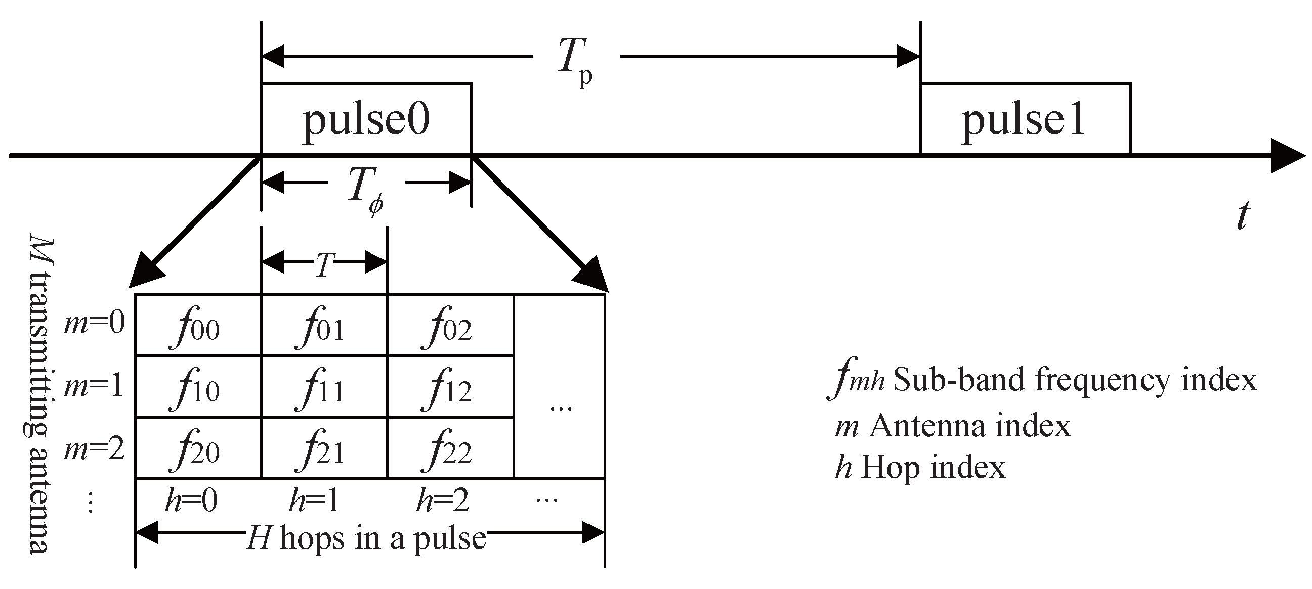
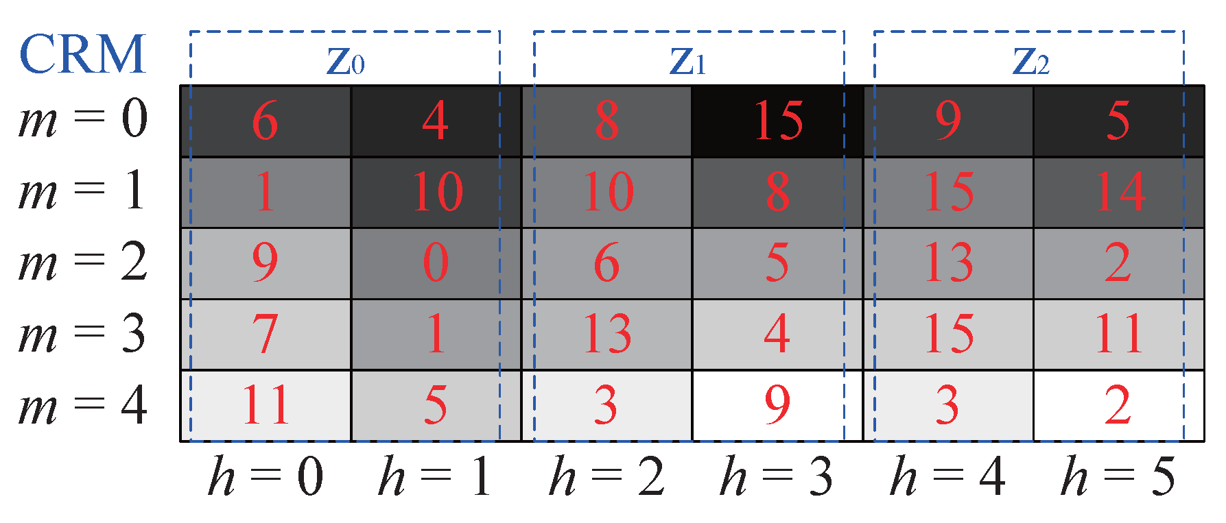
2.1.1. FH-MIMO Radar

In FH-MIMO pulse radars, each pulse is divided into multiple sub-pulses, and each transmitting antenna emits sub-pulses at different frequency codes simultaneously, enabling parallel transmission. The structure of the transmitted waveform is illustrated in Figure 1.

Here, $T_{\mathrm{p}}$ represents the Pulse Repetition Time (PRT) of the FH-MIMO waveform. The system employs M transmitting antennas, with each radar pulse consisting of H sub-pulses, each of duration T, so the total pulse duration is $T_{\varphi }=HT$. The signal bandwidth B is divided into K sub-carriers, meaning there are K available frequency codes. The baseband frequency of the kth sub-carrier is given by the following:

$$\begin{array}{c}\hfill f_k={\displaystyle \frac{\left(⌊-\frac{K}{2}⌋+k\right)B}{K}},(k=0,1,\cdots ,K-1),\end{array}$$

(1)

where $⌊·⌋$ denotes the floor function.

The frequency spacing between sub-carriers is

$$\begin{array}{c}\hfill {\mathrm{\Delta }}_f={\displaystyle \frac{B}{K}},BT/K\in {\mathbb{I}}_{+},\end{array}$$

(2)

where $\mathbb{I}+$ represents the set of positive integers, and the condition $BT/K=T{\mathrm{\Delta }}_f\in {\mathbb{I}}_{+}$ ensures that the product of sub-carrier spacing and sub-pulse duration is an integer. From a spectral resolution perspective, the sub-pulse duration T provides a resolution of $1/T$, and the frequency hopping rate is an integer multiple of this resolution to avoid spectral leakage. To maximize the communication rate, ${\mathbb{I}}_{+}$ is typically set to 1, ensuring that the sub-carrier spacing equals the reciprocal of the sub-pulse duration, which is similar to the requirements in Orthogonal Frequency Division Multiplexing (OFDM). For M transmitting antennas, each radar pulse requires a frequency hopping matrix of size $M\times H$. To maintain orthogonality across antennas at any given time—i.e., ensuring that different antennas use distinct frequency codes within the same hop—the number of antennas M and the number of sub-carrier frequencies K must satisfy $M\le K$.

Let the transmission frequency of antenna m in the hth sub-hop be denoted by $f_{hm}$, where $f_{hm}\in f_k$ and $k\in [0,K-1]$. The FH waveform for the m-th transmitting antenna is then

$$\begin{array}{c}\hfill s_m\left(t\right)=\sum _{h=1}^H{e}^{\mathrm{j}2\pi f_{hm}t}u(t-hT),m=0,1,\cdots ,M-1,\end{array}$$

(3)

where $u\left(t\right)$ is a rectangular function with a duration T:

$$u\left(t\right)=\left\{\begin{array}{ccc}\hfill 1& ,\hfill & \hfill 0<t<T\\ \hfill 0& ,\hfill & \hfill \mathrm{otherwise}\end{array}\right..$$

(4)

To ensure orthogonality between the antennas in the same sub-hop, the signals transmitted by different antennas must satisfy the orthogonality condition:

$$\begin{array}{c}\hfill \int s_m\left(t\right)s_{m^{\prime }}^{*}\left(t\right)\mathrm{d}t=0,m\ne m^{\prime }.\end{array}$$

(5)

where ${(·)}^{*}$ denotes the complex conjugate.

2.1.2. FHCS-MIMO DFRC

To achieve information embedding in the FHCS-MIMO DFRC system, each transmission sub-hop embeds communication information by selecting different combinations of frequency-hopping codes. This allows simultaneous radar and communication functionality. Let i represent the pulse index. The transmitted signal for each sub-hop is the superposition of signals from M transmitting antennas, and the waveform for sub-hop h can then be expressed as

$$\begin{array}{c}\hfill s_{hi}\left(t\right)=\sum _{m=0}^{M-1}{e}^{\mathrm{j}2\pi f_{hmi}t}u(t-hT).\end{array}$$

(6)

For a system with K available frequency codes, M distinct codes were selected for each sub-hop, which can be understood as a combination problem. Specifically, M frequency codes were chosen from K, yielding $C_K^M$ unique combinations. These combinations formed the FHCS communication symbol set. Without loss of generality, it was assumed that the frequency codes transmitted by different antennas within each sub-hop were sorted as follows:

$$\begin{array}{c}\hfill f_{h0}<f_{h1}<\cdots <f_{h(M-1)}.\end{array}$$

(7)

Each combination corresponds to an FHCS communication symbol, representing one or more bits of information. The total number of unique FHCS communication symbols is

$$\begin{array}{c}\hfill L_{\mathrm{FHCS}}=C_K^M={\displaystyle \frac{K!}{M!(K-M)!}}.\end{array}$$

(8)

Since $L_{\mathrm{FHCS}}$ is not necessarily a power of 2, the communication symbol dictionary is usually truncated to the nearest integer power of 2. Thus, the maximum number of bits that each FHCS communication symbol (i.e., each sub-hop) can represent is

$$\begin{array}{c}\hfill N_{\mathrm{FHCS}}=⌊{log}_2\left(C_K^M\right)⌋.\end{array}$$

(9)

2.1.3. QAM-FHCS-MIMO DFRC

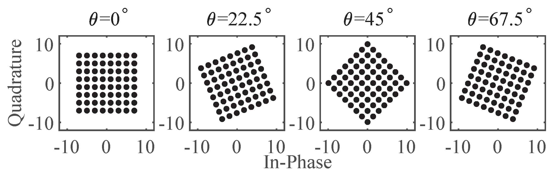
QAM can be viewed as a combination of ASK and PSK modulation [31]. By leveraging both the phase and amplitude of the signal, QAM increases the amount of information transmitted per unit of bandwidth. Let ${\mathcal{Q}}_{hmi}$ represent the transmission signal of the m-th transmitting antenna using $\mathcal{M}$-QAM modulation in the h-th sub-hop of the ith pulse. The transmission signal for QAM-FHCS-MIMO DFRC in sub-hop h is then expressed as

$$\begin{array}{c}\hfill s_{hi}\left(t\right)=\sum _{m=0}^{M-1}{\mathcal{Q}}_{hmi}{e}^{-\mathrm{j}2\pi f_{hmi}t}u(t-hT).\end{array}$$

(10)

For $\mathcal{M}$-QAM modulation, the maximum number of bits that can theoretically be transmitted by each sub-pulse is

$$\begin{array}{c}\hfill N_{\mathrm{QAM}}=M{log}_2\mathcal{M}.\end{array}$$

(11)

2.2. CRM Principles

As illustrated in Figure 2, the 64-QAM constellation can be rotated at four distinct angles, resulting in four unique constellation diagrams. By using these four states, two bits of information can be represented.

The number of possible rotation states determines the order of CRM. Figure 2 shows the constellation diagram with four rotation states corresponds to four CRM symbols. Each CRM symbol consists of multiple QAM constellation point samples. Demodulation of CRM relies on estimating the rotation state of the constellation from these samples. To simplify the description, assume that each CRM symbol contains $L=M{H}_{\mathrm{c}}$ samples, where M is the number of transmitting antennas, and $H_{\mathrm{c}}$ is the number of sub-hops with the same rotation state. Based on this setup, CRM can be viewed as a sub-dimensional modulation technique that can coexist with FHCS and QAM. FHCS transmits information through frequency code combinations of different antennas, while QAM modulates the phase and amplitude in each sub-hop. CRM utilizes the rotated constellation diagrams of L QAM symbols for information transmission. Figure 3 illustrates the process of superimposing CRM with FHCS and QAM. In this figure, m and h represent the indices of the transmitting antenna and sub-hop, respectively. Each column shows the frequency code sorting of FHCS modulation, with numbers 0∼15 indicating 16-QAM symbols, while $z_0$∼$z_2$ above each sub-hop represents CRM symbol states.

Assuming there are Y possible rotation states for the constellation diagram, which corresponds to the CRM modulation order, the symbol set for CRM is $\mathrm{\Theta }={[{\theta }_0,{\theta }_1,\cdots ,{\theta }_{(Y-1)}]}^{\mathrm{T}}$. The total number of sub-hops per pulse H and the number of sub-hops per CRM symbol $H_{\mathrm{c}}$ must be an integer multiple, i.e., $H/H_{\mathrm{c}}=Z$, where Z is a positive integer. According to the signal model described in [32], the CRM-QAM-FHCS-MIMO DFRC signal model for each pulse is given by

$$\begin{array}{c}\hfill s\left(t\right)=\sum _{z=0}^{Z-1}{e}^{\mathrm{j}{\theta }_z}\sum _{h=0}^{H-1}\sum _{m=0}^{M-1}{\beta }_{hm}{\mathcal{Q}}_{hm}{e}^{\mathrm{j}2\pi f_{hm}t}u(t-hT)+w\left(t\right),\end{array}$$

(12)

where $z=\lfloor h/H_{\mathrm{c}}\rfloor$ is the CRM symbol index, $e^{\mathrm{j}{\theta }_z}({\theta }_z\in \mathrm{\Theta })$ is the CRM modulation term, ${\beta }_{hm}$ is the channel coefficient, $\mathcal{Q}hm$ is the QAM symbol, $e^{\mathrm{j}2\pi fhmt}$ is the FHCS modulation term, $u\left(t\right)$ is a rectangular function of duration T, and $w\left(t\right)$ is the noise term.

Each CRM symbol state ${\theta }_z$ has Y possible values. For a pulse with $H=Z{H}_{\mathrm{c}}$ sub-hops, CRM can represent Z bits of Y-ary data, yielding $Y^Z$ combinations of rotation states. Therefore, the number of bits that CRM modulation can carry per pulse is

$$\begin{array}{c}\hfill N_{\mathrm{CRM}}=⌊{log}_2{Y}^Z⌋=⌊Z{log}_{2}Y⌋.\end{array}$$

(13)

When CRM, $\mathcal{M}$-QAM, and FHCS modulations coexist, the maximum number of bits that each pulse can carry, according to Equations (9), (11) and (13), is

$$\begin{array}{c}\hfill N_{\mathrm{data}}=\underset{\mathrm{CRM}}{\underbrace{⌊Z{log}_{2}Y⌋}}+\underset{\mathrm{QAM}}{\underbrace{HM{log}_2\mathcal{M}}}+\underset{\mathrm{FHCS}}{\underbrace{H⌊{log}_2\left(C_K^M\right)⌋}}.\end{array}$$

(14)

where $\mathcal{M}$ is the order of QAM, and K is the number of sub-carrier frequencies.

2.3. Principles of Demodulation

During demodulation, the parameters of different modulation schemes are interdependent, requiring a specific order to accurately extract the information embedded in each dimension. A step-by-step demodulation approach is employed, progressing from the simplest to the most complex. Assuming that channel errors have been accurately estimated and compensated (refer to [32] for channel correction methods), we first perform FHCS demodulation as it mainly relies on frequency and is less affected by amplitude, phase, or rotation angles. Next, the constellation’s rotation state is estimated using amplitude and phase information from each sub-hop to demodulate the CRM information. Finally, after compensating for the CRM rotation, QAM demodulation is performed to retrieve the transmitted symbols. Therefore, the process consists of three levels of demodulation, where each level depends on the accurate demodulation of the preceding one.

2.3.1. FHCS Demodulation

From the concept of FHCS, it can be seen that its demodulation is relatively simple. It involves performing a Discrete Fourier Transform (DFT) on the echo data, extracting the M peaks with the largest amplitudes and arranging the corresponding frequency codes according to the sorting rule in (7). This provides the frequency code combination $D_{\mathrm{FHCS}}$ for the M transmitting antennas.

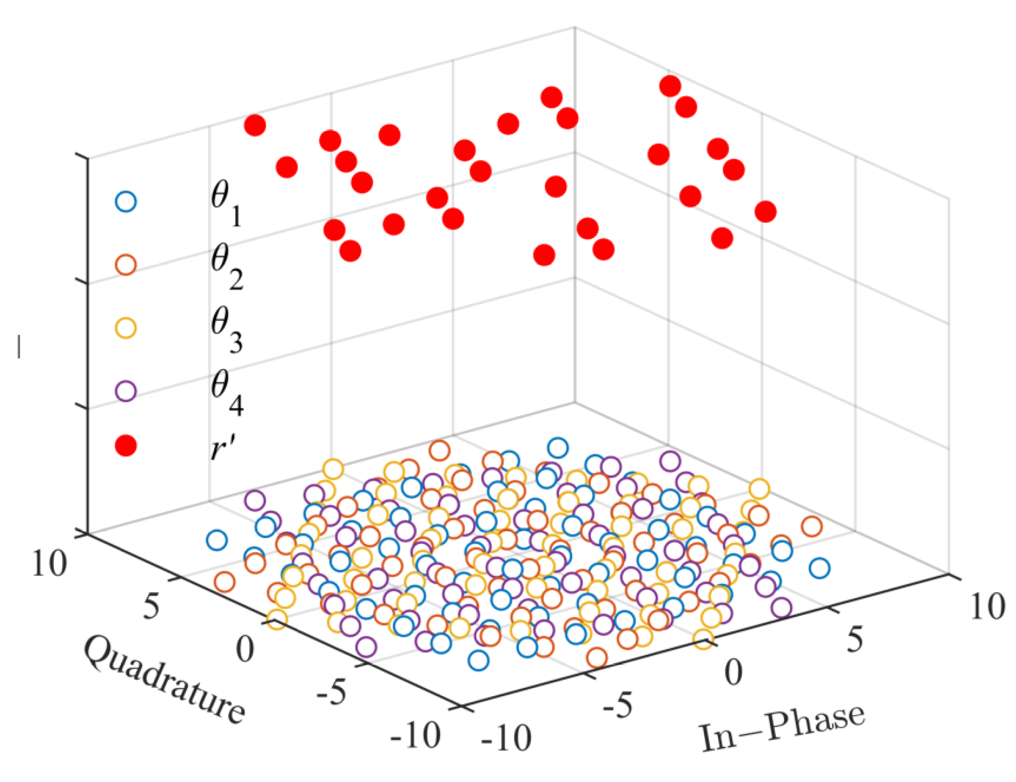
2.3.2. CRM Demodulation

CRM demodulation involves estimating the rotation state of the constellation diagram based on L observed samples. In the process of communication error analysis, we often use the normal distribution model, so we can use the least squares method to estimate the CRM rotation angle $\theta$. In typical QAM modulation (where noise is uncorrelated and all symbols are equally likely), let the transmitted $\mathcal{M}$-QAM symbol set be $\mathbf{s}={[s_0,s_1,\cdots ,s_{\mathcal{M}-1}]}^{\mathrm{T}}$, which corresponds to $\mathcal{M}$ constellation points. If the CRM rotation angle is ${\theta }_y$, the sample subset of the CRM symbol is expressed as

$$\begin{array}{c}\hfill {\mathbf{s}}^{\prime }\left({\theta }_y\right)=e^{\mathrm{j}{\theta }_y}\mathbf{s},{\theta }_y\in \mathrm{\Theta }.\end{array}$$

(15)

The total CRM symbol set, including all rotation states, is

$$\begin{array}{c}\hfill {\mathcal{S}}^{\prime }=\left[{\mathbf{s}}^{\prime }\left({\theta }_0\right),{\mathbf{s}}^{\prime }\left({\theta }_1\right),\cdots ,{\mathbf{s}}^{\prime }\left({\theta }_{(Y-1)}\right)\right].\end{array}$$

(16)

Considering noise, a CRM symbol, represented as the vector of L QAM symbols under the same rotation, is

$$\begin{array}{c}\hfill {\mathbf{r}}^{\prime }={\mathbf{s}}_L^{\prime }\left({\theta }_y\right)+{\mathbf{w}}_L,{\theta }_y\in \mathrm{\Theta },\end{array}$$

(17)

where the vector ${\mathbf{s}}_L^{\prime }\left({\theta }_y\right)$ represents L elements received from the symbol subset ${\mathbf{s}}^{\prime }\left({\theta }_y\right)$, and $\mathbf{w}L$ is the noise vector of length L.

To determine the most likely rotation state $\theta$ from the L observed symbols ${\mathbf{r}}^{\prime }={\left[r_0^{\prime },r_1^{\prime },\cdots ,r_{(L-1)}^{\prime }\right]}^{\mathrm{T}}$, we calculated the Euclidean distance between each received symbol $r_l^{\prime }$ and the corresponding symbols in all possible rotated constellations:

$$\begin{array}{c}\hfill d_l\left(\theta \right)=min\{\parallel r_l^{\prime }-{\mathbf{s}}^{\prime }\left(\theta \right)\parallel \},{\mathbf{s}}^{\prime }\left(\theta \right)\in {\mathcal{S}}^{\prime },r_l^{\prime }\in {\mathbf{r}}^{\prime },\end{array}$$

(18)

where $\parallel ·\parallel$ denotes the minimum Euclidean distance. Using the least squares method, we combined the distances for all samples to estimate the most likely rotation state. Substituting $d_l\left(\theta \right)$ into the least squares cost function $\mathcal{L}\left(\theta \right)$, we solved the following:

$$\begin{array}{c}\hfill \begin{array}{cc}\hfill \widehat{\theta }& =arg\underset{\theta }{min}\mathcal{L}\left(\theta \right)\iff arg\underset{\theta \in \mathrm{\Theta }}{min}\sum _{l=0}^{L-1}{\parallel d_l\left(\theta \right)\parallel }^2.\hfill \end{array}\end{array}$$

(19)

Since the possible rotation angles $\theta \in \mathrm{\Theta }$ are finite, a simple exhaustive search can be used to find the optimal estimate $\widehat{\theta }$, which corresponds to the CRM modulation result.

2.3.3. QAM Demodulation

Once the CRM rotation angle $\theta$ is estimated, we compensate for this rotation to obtain the original QAM symbols. The compensated QAM symbols are given by

$$\begin{array}{c}\hfill \widehat{\mathbf{s}}=e^{-\mathrm{j}\widehat{\theta }}{\mathbf{r}}^{\prime }.\end{array}$$

(20)

QAM demodulation then involves finding the closest symbol in the QAM constellation $\mathbf{s}$ to each compensated symbol ${\widehat{s}}_{hm}$. This is conducted by minimizing the Euclidean distance:

$$\begin{array}{c}\hfill {\tilde{s}}_{hm}=arg\underset{s\in \mathbf{s}}{min}\{\parallel {\widehat{s}}_{hm}-s\parallel \},\end{array}$$

(21)

where ${\widehat{s}}_{hm}$ is the element at position $hm$ in the compensated symbol matrix.

2.4. Low-Complexity Fast CRM Demodulation

In Section 2.3.2, we introduced a standard CRM demodulation method that requires an exhaustive search over all possible rotation states, leading to high computational complexity. To reduce this complexity, we propose an approach that estimates the rotation state using only the constellation points in the first quadrant. Additionally, by taking the modulus of the real and imaginary parts of the CRM symbol samples, we can effectively fold the constellation diagram into the first quadrant. For example, folding the four symbols from Figure 2 into the first quadrant yields the results shown in Figure 4. In this folded constellation, the projection positions of the constellation points in the first quadrant on the x-axis and y-axis have significant differences. The projection coordinates of the unrotated constellation points have only a few fixed values. For example, after folding the 64QAM constellation diagram, there are only four fixed values (1, 3, 5, and 7). In contrast, the projection coordinates after rotation are more dispersed. Therefore, based on the discrete characteristics of the projection points on the coordinate axes, the rotation state of the constellation points can be quickly determined.

After the constellation diagram is folded, let the projection coordinates of L CRM symbol samples ${\mathbf{r}}^{\prime }$ on the x-axis be ${\mathbf{r}}_x^{\prime }$. Using the known set of CRM rotation angles $\mathrm{\Theta }$, compensate ${\mathbf{r}}_x^{\prime }$ to obtain Y sets of compensated results ${\mathbf{r}}_x^{\prime }\left({\theta }_y\right)$, where ${\theta }_y\in \mathrm{\Theta }$. Let the fixed positions corresponding to the projection coordinates of the unrotated constellation points be $\mathbf{p}$. Similar to (18), we can obtain

$$\begin{array}{c}\hfill d_{lx}\left(\theta \right)=min\{\parallel r_x^{\prime }\left({\theta }_y\right)-\mathbf{p}\parallel \},r_x^{\prime }\in {\mathbf{r}}_x^{\prime },{\theta }_y\in \mathrm{\Theta }.\end{array}$$

(22)

Then, based on the minimum cumulative Euclidean distance of the L samples from the reference position $\mathbf{p}$, the final constellation rotation angle is estimated.

$$\begin{array}{c}\hfill \begin{array}{c}\hfill \widehat{{\theta }_x}=arg\underset{\theta \in \mathrm{\Theta }}{min}\sum _{l=0}^{L-1}{\parallel d_{lx}\left(\theta \right)\parallel }^2.\end{array}\end{array}$$

(23)

Unlike (18), in (22), the projection position vector $\mathbf{p}$ is used to replace the constellation diagram ${\mathbf{s}}^{\prime }\left(\theta \right)$ under the rotation of angle $\theta$. As a result, the matching range is greatly reduced, and the computational complexity is lowered. Compared with (19), the number of summations in (23) remains unchanged. Therefore, the computational load of this step is the same under both methods. Moreover, the summation of squares here can be further simplified to the summation of magnitudes, which can further simplify the computation.

Lemma 1.

Let $\mathcal{K}=\mathcal{M}/4$ represent the number of unique points in the first quadrant of an $\mathcal{M}$-QAM constellation. The probability $P\left(L\right)$ that all $\mathcal{K}$ points are sampled at least once in L independent trials is

$$\begin{array}{c}\hfill P\left(L\right)={\left(1-{\left(1-{\displaystyle \frac{1}{\mathcal{K}}}\right)}^L\right)}^{\mathcal{K}}.\end{array}$$

(24)

Proof. 

The probability of selecting a specific point in one trial is ${\displaystyle \frac{1}{\mathcal{K}}}$. The probability of not selecting that point in one trial is $1-{\displaystyle \frac{1}{\mathcal{K}}}$. Over L trials, the probability of never selecting that point is ${\left(1-{\displaystyle \frac{1}{\mathcal{K}}}\right)}^L$. The complement of this probability gives the chance of selecting the point, at least once, $1-{\left(1-{\displaystyle \frac{1}{\mathcal{K}}}\right)}^L$. To ensure that all $\mathcal{K}$ points are sampled at least once, this must happen independently for each point. Therefore, the probability of sampling all $\mathcal{K}$ points at least once in L trials is (24). □

Based on the description of (24) in the Lemma 1, after folding the constellation diagram, the number of constellation points in the first quadrant is $\mathcal{K}$. As L increases, the probability that each constellation point is sampled will tend to 1. Consequently, the reliability of estimating the rotation angle of the CRM based on the complete shape of the constellation diagram is significantly enhanced.

Compare the differences in steps and computational complexity between these two methods. Each CRM symbol has L samples. In the method described in Section 2.3.2, based on (18), each sample requires the calculation of $\mathcal{M}Y$ Euclidean distances, with a computational complexity of $\mathcal{O}\left(\mathcal{M}YL\right)$ resulting in a three-dimensional data array of size $\mathcal{M}YL$. For each constellation rotation state, among the $\mathcal{M}$ constellation points, the minimum Euclidean distance is found, resulting in a two-dimensional data array of size $YL$. Let the computational complexity for sorting be $\mathcal{O}({\mathcal{O}}_{\mathcal{S}}\left(\mathcal{M}\right)·YL)$, where ${\mathcal{O}}_{\mathcal{S}}\left(\mathcal{M}\right)$ represents the computational complexity for sorting a data array of length $\mathcal{M}$ once, and this process is repeated $YL$ times. After sorting, based on (19), the L minimum Euclidean distances for each rotation state are summed to obtain a vector of size Y with a computational complexity of $\mathcal{O}\left(L\right)$. Finally, the Y rotation states are sorted to find the minimum value, which is the demodulation result. The computational complexity for this part is ${\mathcal{O}}_{\mathcal{S}}\left(Y\right)$.

Table 1. Comparison of computational complexity.

Step	Traditional Method	Folding Method
Calculating Euclidean Distance	$\mathcal{O}\left(\mathcal{M}YL\right)$	$\mathcal{O}\left(pYL\right)$
Finding the Minimum Value	$\mathcal{O}({\mathcal{O}}_{\mathcal{S}}\left(\mathcal{M}\right)·YL)$	$\mathcal{O}({\mathcal{O}}_{\mathcal{S}}\left(p\right)·YL)$
Accumulating Euclidean Distances	$\mathcal{O}\left(L\right)$	$\mathcal{O}\left(L\right)$
Sorting	${\mathcal{O}}_{\mathcal{S}}\left(Y\right)$	${\mathcal{O}}_{\mathcal{S}}\left(Y\right)$

Note: M, p, Y, and L correspond to different variables in the main text, respectively. ${\mathcal{O}}_S$ denotes the sorting complexity. The above steps of these two methods correspond to Equations (18), (19), (22), and (23), respectively.

lists the differences in computational complexity for the various steps between the two methods. In fact, the proposed Low-Complexity Fast CRM Demodulation method is similar in steps to the first method. However, after folding the constellation diagram and projecting, the Euclidean distance calculation space can be reduced from the number of constellation points $\mathcal{M}$ to the number of projection points $\mathbf{p}$, thus significantly reducing the computational complexity in subsequent steps. For example, following the application of the folding technique to 64QAM, the computation is reduced from 64 constellation points to 4 projection points, as depicted in the leftmost illustration of Figure 4. Under these circumstances, the computational speed can be enhanced by approximately a factor of 16. Moreover, the cache size of data blocks at each stage can also be correspondingly reduced.

3. Radar Performance Analysis

Although CRM based on QAM can improve communication bandwidth, it disrupts the constant modulus property of the transmitted signal, which can impact radar detection capability. It is essential to evaluate how the proposed method affects radar performance. Radar detection capability and ambiguity function performance are two critical indicators for assessing radar system performance. Detection capability determines the radar’s ability to identify targets, while the ambiguity function influences target resolution and anti-interference performance. Therefore, we will analyze the effects of the proposed modulation method on both of these aspects.

3.1. Detection Capability

Compared to PSK modulation, QAM generally provides better communication performance at the same signal-to-noise ratio (SNR). However, the non-constant modulus property of QAM increases the Peak-to-Average Power Ratio (PAPR) as the modulation order increases:

$$\begin{array}{c}\hfill \mathrm{PAPR}={\displaystyle \frac{\mathrm{Peak}\mathrm{Power}}{\mathrm{Average}\mathrm{Power}}}.\end{array}$$

(25)

With a fixed maximum output power, the average power of the QAM-modulated signal is lower than that of a constant modulus signal, leading to a reduction in radar detection range. According to the radar range equation [33], the maximum radar detection range is proportional to the fourth root of the transmitted power:

$$\begin{array}{c}\hfill R_{max}\propto P_{\mathrm{t}}^{{\displaystyle \frac{1}{4}}}.\end{array}$$

(26)

By normalizing the transmitted power and detection range, Figure 5 illustrate how the transmitted power $P_{\mathrm{t}}$ and detection range $R_{max}$ vary with changes in the QAM modulation order. It can be seen that the maximum detection range is approximately $R_{max}\propto {\left[{\displaystyle \frac{1}{\mathrm{PAPR}}}\right]}^{{\displaystyle \frac{1}{4}}}$. As the order of QAM modulation increases, the normalized detection distance gradually decreases and eventually stabilizes. When the QAM modulation order M is an odd power of 2, the constellation diagram of QAM takes on a “cross” shape, with a normalized detection distance of 0.8. When the QAM modulation order M is an even power of 2, the constellation diagram of QAM is square-shaped, with a normalized detection distance of 0.76. The difference in constellation diagram shapes due to odd and even powers leads to a fluctuating decrease in normalized transmission power. When the QAM modulation order is $M\le 4$, the radar supports saturated power transmission, which does not affect the radar’s detection capability. When $4<M<1024$, the radar’s detection capability significantly decreases, and when $M>1024$, the impact on radar detection performance becomes less sensitive. In contrast, the communication data rate increases linearly with the modulation order, carrying more bits. Therefore, in practical applications, a balance should be struck between radar detection capability and communication performance requirements.

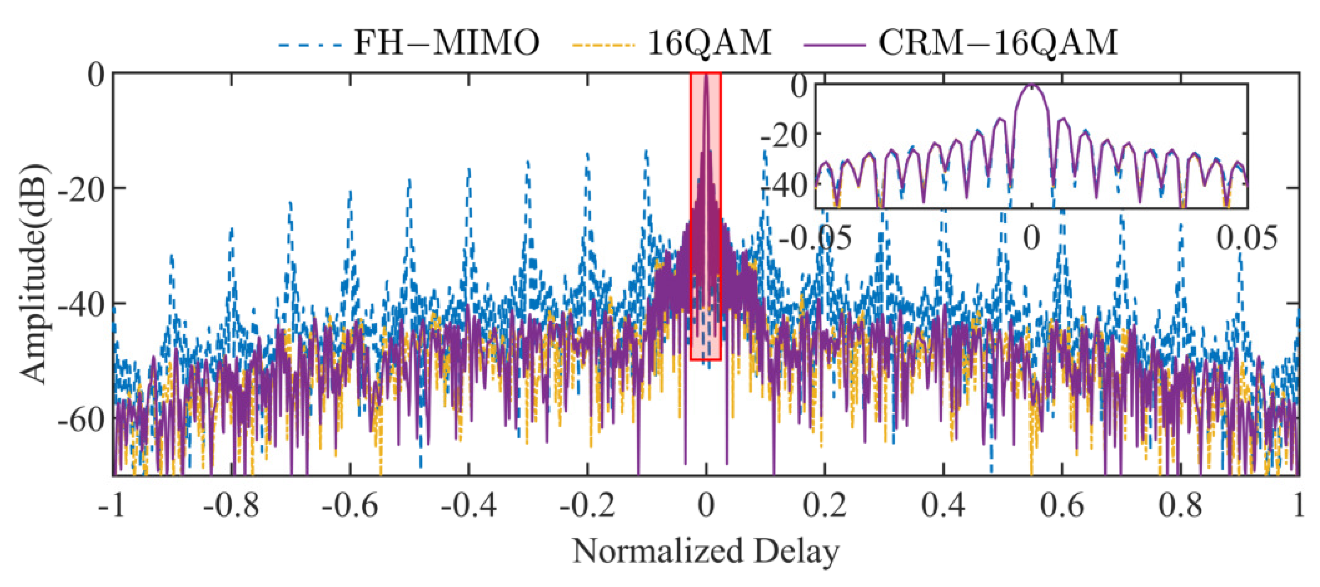
3.2. Ambiguity Function

For Single-Input Multiple-Output (SIMO) radar systems, the ambiguity function [34] is defined as

$$\begin{array}{c}\hfill \chi (\tau ,v)\stackrel{\mathrm{\Delta }}{=}\left|\int s\left(t\right)s^{*}(t-\tau )e^{-j2\pi vt}dt\right|,\end{array}$$

(27)

where $s\left(t\right)$ represents the radar transmission waveform and v denotes the Doppler frequency. This two-dimensional function can be understood as the output of the matched filter in the receiver when there are varying degrees of mismatch in delay $\tau$ and Doppler frequency v.

In MIMO radar systems, the multi-antenna configuration introduces the impact of spatial resolution. Consequently, the radar ambiguity function must consider not only time and frequency matching, but also spatial frequency matching for target identification and resolution. To illustrate this, we considered a uniform linear array. Let M represent the number of transmitting antennas with element spacing $d_{\mathrm{t}}$, and let N represent the number of receiving antennas with spacing $d_{\mathrm{r}}$. For a target at angle $\theta$, the transmitted waveform is

$$\begin{array}{c}\hfill s_{\mathrm{t}}\left(t\right)=\sum _{m=0}^{M-1}{s}_m\left(t\right)e^{j{\displaystyle \frac{2\pi m{d}_{\mathrm{t}}sin\left(\theta \right)}{\lambda }}},\end{array}$$

(28)

where $s_m\left(t\right)$ is the signal transmitted by the m-th antenna. The echo received by the n-th antenna is

$$\begin{array}{c}\hfill s_n\left(t\right)=\sum _{m=0}^{M-1}{s}_m(t-\tau )e^{2\pi vt}{e}^{j{\displaystyle \frac{2\pi m{d}_{\mathrm{t}}sin\left(\theta \right)}{\lambda }}}{e}^{j{\displaystyle \frac{2\pi n{d}_{\mathrm{r}}sin\left(\theta \right)}{\lambda }}}.\end{array}$$

(29)

The three exponential terms in this equation represent the Doppler frequency offset, the phase variation introduced by the transmitting antenna, and the phase variation introduced by the receiving antenna, respectively. Similar to the Nyquist sampling theorem [35], the spatial sampling theorem states that, to sample a signal without aliasing, the sampling frequency must be greater than or equal to twice the input signal. For a uniform linear array, its spatial sampling spacing $d_{\mathrm{r}}$ determines the sampling frequency, i.e., the spatial sampling frequency is $f_{\mathrm{s}}={\displaystyle \frac{c}{d_{\mathrm{r}}}}$, where c is the speed of electromagnetic wave propagation. The projection frequency of the target echo signal on the uniform sampling linear array is $f={\displaystyle \frac{c}{\lambda }}sin\left(\theta \right)$. Normalizing the frequency component of the target along the linear array, the normalized spatial frequency is

$$\begin{array}{c}\hfill f_{\theta }\stackrel{\mathrm{\Delta }}{=}{\displaystyle \frac{f}{f_{\mathrm{s}}}}={\displaystyle \frac{d_{\mathrm{r}}}{\lambda }}sin\left(\theta \right).\end{array}$$

(30)

Substituting the expression for $f_{\theta }$ into the equation for $s_n\left(t\right)$, we can rewrite the received signal as

$$\begin{array}{c}\hfill s_n^{\tau ,v,f_{\theta }}\left(t\right)=\sum _{m=0}^{M-1}{s}_m(t-\tau )e^{2\pi vt}{e}^{j2\pi f_{\theta }(\gamma m+n)},\end{array}$$

(31)

where $\gamma \stackrel{\mathrm{\Delta }}{=}{\displaystyle \frac{d_{\mathrm{t}}}{d_{\mathrm{r}}}}$. Similar to SIMO radar systems, the ambiguity function for MIMO radar systems can be understood as the output of the matched filter in the receiver when there are varying degrees of mismatch in delay ($\tau$), Doppler frequency (v), and spatial frequency ($f_{\theta }$). The specific result is

$$\begin{array}{c}\hfill \begin{array}{cc}\hfill & \sum _{n=0}^{N-1}{\int }_{-\infty }^{+\infty }{s}_n^{\tau ,v,f_{\theta }}\left(t\right)·{\left(s_n^{{\tau }^{\prime },v^{\prime },f_{\theta }^{\prime }}\left(t\right)\right)}^{*}dt\hfill \\ \hfill & =\left(\sum _{n=0}^{N-1}{e}^{j2\pi (f_{\theta }-f_{\theta }^{\prime })n}\right)\left(\sum _{m=0}^{M-1}\sum _{m^{\prime }=0}^{M-1}{\int }_{-\infty }^{+\infty }{s}_m(t-\tau )s_{m^{\prime }}^{*}(t-{\tau }^{\prime })e^{j2\pi (v-v^{\prime })t}dt·e^{j2\pi (m{f}_{\theta }-m^{\prime }{f}_{\theta }^{\prime })\gamma }dt\right).\hfill \end{array}\end{array}$$

(32)

In this equation, the first term on the right represents the spatial beam pointing matching, which is independent of the specific transmitted waveform. The second part describes the impact of delay ($\tau$), Doppler frequency (v), and spatial frequency ($f_{\theta }$) on range resolution, velocity resolution, and spatial angle resolution. Therefore, the ambiguity function of MIMO radar can be defined as

$$\begin{array}{c}\hfill \begin{array}{c}\hfill \chi (\tau ,v,f_{\theta },f_{\theta }^{\prime })\stackrel{\mathrm{\Delta }}{=}\sum _{m=0}^{M-1}\sum _{m^{\prime }=0}^{M-1}{\chi }_{m,m^{\prime }}(\tau ,v)e^{j2\pi (m{f}_{\theta }-m^{\prime }{f}_{\theta }^{\prime })\gamma },\end{array}\end{array}$$

(33)

where

$$\begin{array}{c}\hfill \begin{array}{c}\hfill {\chi }_{m,m^{\prime }}(\tau ,v)\stackrel{\mathrm{\Delta }}{=}{\int }_{-\infty }^{+\infty }{s}_m\left(t\right)s_{m^{\prime }}^{*}(t+\tau )e^{j2\pi vt}dt.\end{array}\end{array}$$

(34)

The exponential term $e^{j2\pi (m{f}_{\theta }-m^{\prime }{f}^{\prime }\theta )\gamma }$ can be interpreted as the variation caused by spatial frequency mismatch between signals from different transmitting antennas. Since this expression does not hold for different transmitting antennas ($m\ne m^{\prime }$), the content of $\chi m,m^{\prime }(\tau ,v)$ is similar to the ambiguity function of SIMO radar. When $m=m^{\prime }$, it reduces to the standard SIMO ambiguity function. The cross-ambiguity function is defined to describe the matching between two waveforms $s_m$ and $s_{m^{\prime }}$. Based on (12), let I be the number of coherent pulse accumulations. Then, the I pulses from each transmitting antenna under CRM-QAM can be expressed as

$$\begin{array}{c}\hfill \begin{array}{c}\hfill s_m\left(t\right)=\sum _{i=0}^{I-1}{\varphi }_{mi}^{\mathrm{CRM}}(t-i{T}_{\mathrm{p}})·\mathrm{rect}\left({\displaystyle \frac{t-i{T}_{\mathrm{p}}}{T_{\varphi }}}\right),\end{array}\end{array}$$

(35)

where i represents the Pulse Repetition Time (PRT) index, and $\mathrm{rect}(·)$ is the rectangular function, which takes a value of 1 when $t\in [0,T_{\varphi }]$ and 0 otherwise. The transmission signal of antenna m in each pulse is

$$\begin{array}{c}\hfill {\varphi }_{mi}^{\mathrm{CRM}}\left(t\right)=\sum _{z=0}^{Z-1}{e}^{\mathrm{j}{\theta }_n}\sum _{h=0}^{H-1}{\mathcal{Q}}_{hmi}{e}^{\mathrm{j}2\pi f_{hmi}t}u(t-hT).\end{array}$$

(36)

Substitute (35) and (36) into (34), respectively. Taking into account the matching of signals between different Pulse Repetition Times (PRTs), the problem becomes complex, especially when there is range ambiguity, and the relevant methods provided in [36] can be referred to. Disregarding the range ambiguity, that is, considering only the matching between the transmitted signal and the echo signal within the current pulse period, the general ambiguity function expression for CRM-QAM-FHCS-MIMO DFRC can be derived as follows:

$$\begin{array}{c}\hfill \begin{array}{cc}\hfill {\chi }^{\mathrm{CRM}}(\tau ,v,f_{\theta },f_{\theta }^{\prime })& =\sum _{l=0}^{I-1}{e}^{j2\pi vl{T}_{\mathrm{p}}}\sum _{z=0}^{Z-1}\sum _{z^{\prime }=0}^{Z-1}{e}^{\mathrm{j}({\theta }_{zl}-{\theta }_{z^{\prime }l})}\hfill \\ \hfill & \times \sum _{m=0}^{M-1}\sum _{m^{\prime }=0}^{M-1}\sum _{h=0}^{H-1}\sum _{h^{\prime }=0}^{H-1}{\mathcal{Q}}_{hml}{\mathcal{Q}}_{h^{\prime }{m}^{\prime }l}^{*}{r}_{h,h^{\prime },m,m^{\prime },l}^{\varphi }\left(\tau \right)e^{j2\pi (m{f}_{\theta }-m^{\prime }{f}_{\theta }^{\prime })\gamma },\hfill \end{array}\end{array}$$

(37)

where $r^{\varphi }$ is the cross-correlation function of the signals transmitted by different antennas. In (37), $e^{\mathrm{j}({\theta }_{zl}-{\theta }_{z^{\prime }l})}$ represents the impact caused by the mismatch condition of CRM.

The ambiguity functions of the waveforms for FHCS-MIMO, 16QAM-FHCS-MIMO, and CRM-16QAM-FHCS-MIMO were simulated, with the zero-Doppler cut results shown in Figure 6. From the local magnified view, it can be observed that these three waveforms exhibited nearly identical ambiguity functions near zero delay. Over the entire range of time delays, the FHCS-MIMO waveform displayed distinct grating lobes, whereas the waveforms with superimposed QAM modulation or CRM-QAM modulation had ambiguity functions that were nearly identical and highly desirable, with virtually no grating lobes. This improvement is attributed to the introduced modulation, which disrupts the coherence of the grating lobes, thereby enhancing the performance of the ambiguity function.

4. Communication Performance Analysis

Based on the understanding of the principles of CRM information embedding and demodulation methods, CRM demodulation essentially involves estimating the rotation angle $\theta$ of the constellation diagram using L constellation point samples. Therefore, the number of samples and the order of CRM (the number of constellation diagram rotation angles) are crucial for the final demodulation estimation. We know that the constellation diagram of QAM modulation is a symmetric figure in all four directions. Thus, the constellation diagram overlaps once every ${90}^{\circ }$ rotation of $\theta$, which can be understood as a fold occurring every ${90}^{\circ }$. Consequently, the range of the rotation angle $\theta$ can only be limited to $-{45}^{\circ }$∼${45}^{\circ }$.

As shown in Figure 7, the constellation diagram of 64QAM modulation was rotated by the angles $\mathrm{\Theta }=[{\theta }_1,{\theta }_2,{\theta }_3,{\theta }_4]$, resulting in the set of four constellation diagrams depicted in the lower layer of the figure, where each are represented by hollow circles of different colors. A set of sample symbols ${\mathbf{r}}^{\prime }$ that were obtained at a particular moment is indicated by the red solid circles in the upper layer of the figure. The CRM demodulation process involves finding the optimal matching constellation diagram for the sample symbol set ${\mathbf{r}}^{\prime }$ under the set $\mathrm{\Theta }$ according to (19), i.e., the angle $\theta$ for which the sum of Euclidean distances is minimized.

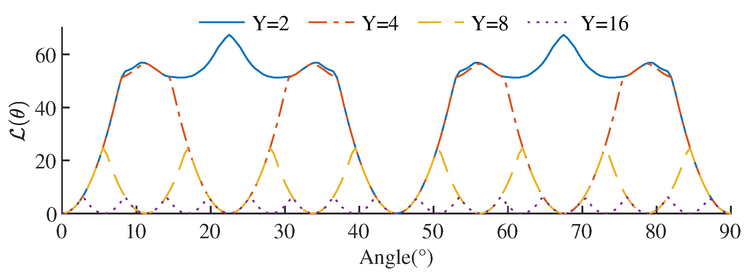
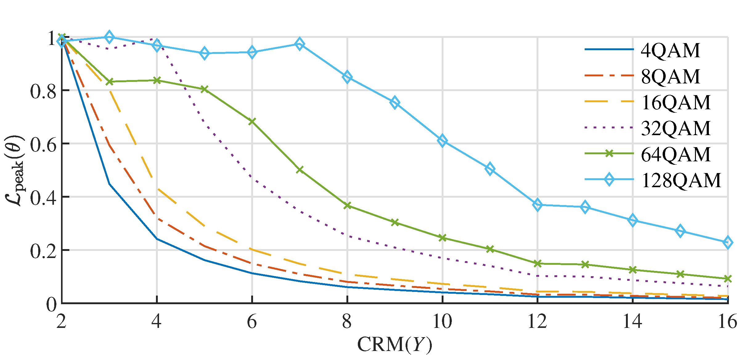
4.1. The Effect of CRM Order on Demodulation Performance

When demodulating the rotation angle $\theta$ of CRM, we aimed to achieve the minimum value (zero point) when the rotation angle matched and a relatively large value (peak) when it did not match. The greater this difference, the better the CRM demodulation performance. Let the number of CRM rotation angles Y be 2, 4, 8, and 16, respectively, with the rotation angles uniformly distributed within a ${90}^{\circ }$ range. Based on (19), CRM demodulation was performed for samples at different rotation angles, yielding the results shown in Figure 8. The x-axis represents the different rotation angles of the received samples, as exemplified in Figure 7. The y-axis represents the cost function $\mathcal{L}\left(\theta \right)$ of the least squares method in (19). From the figure, the following can be observed: (1) when the rotation angle of the sample constellation matches the CRM-set rotation angle, $\mathcal{L}\left(\theta \right)$ tends toward 0, forming a zero point at the CRM-set rotation angle; (2) when the rotation angle of the sample constellation does not match the CRM-set angle, the greater the deviation, and the larger the least squares error $\mathcal{L}\left(\theta \right)$; (3) as the number of rotation angles Y increases, the peak values of $\mathcal{L}\left(\theta \right)$ between each zero point rapidly decrease; and (4) the fewer the number of CRM rotation angles, the more easily identifiable the zero points of $\mathcal{L}\left(\theta \right)$ become.

It can be observed that the modulation order Y of CRM affects the magnitude of the peak value of the cost function $\mathcal{L}\left(\theta \right)$. Figure 9 illustrates the relationship between the normalized ${\mathcal{L}}_{\mathrm{peak}}\left(\theta \right)$ and Y under different QAM modulation orders. The patterns reflected in the curves indicate that the response of ${\mathcal{L}}_{\mathrm{peak}}\left(\theta \right)$ to the superimposed CRM modulation order varies with different QAM modulation orders. For example, under a 64QAM modulation, when $Y>6$, ${\mathcal{L}}_{\mathrm{peak}}\left(\theta \right)$ tends to a smaller value, which implies that the difficulty of CRM demodulation increases. In contrast, under a 4QAM modulation, ${\mathcal{L}}_{\mathrm{peak}}\left(\theta \right)$ tends to a smaller value when the CRM modulation order $Y>4$. Therefore, the optimal CRM modulation order differs when using different QAM modulations.

4.2. The Impact of Sample Size on CRM

Intuitively, as the sample size L increases, the reliability of identifying the rotation state should improve. Therefore, understanding the specific relationship between sample size and the final communication performance is of significant importance for practical engineering applications.

By analyzing the demodulation BER curves under different CRM symbol sample sizes L, a deeper understanding of the impact of various parameters on CRM performance can be achieved. As shown in Figure 10, based on 64QAM modulation, the CRM sample size L starts from 1 and increases stepwise by 5, i.e., $L=[1,6,\cdots ,76]$. It can be observed that, as the number of L increases, the BER tends to stabilize. When $M<10$, the BER is relatively poor and changes dramatically with L. Particularly when $L=1$, accurate identification of the CRM rotation state is only possible under extremely high signal-to-noise ratios (SNR). This is because, after CRM modulation, the constellation points of $\mathcal{M}$ QAM symbols expand to $\mathcal{M}Y$ points, significantly reducing the spacing between each symbol, and this reduction is uneven. Therefore, only under extremely high SNR conditions is it possible to identify the specific rotated constellation point from a single symbol, which is equivalent to $\mathcal{M}Y$-order non-uniform QAM modulation.

5. Simulation Analysis

System simulation of the proposed waveform modulation method enables the emulation of diverse operational conditions and environmental factors, providing a comprehensive analysis of radar performance and communication demodulation performance. This process aids in validating the effectiveness of the proposed method in practical applications. During the radar system simulation, we focused on evaluating the proposed modulation’s capability to resolve target range, velocity, and angle, comparing the radar detection performance differences between the proposed method and existing methods. In the communication system simulation, we analyzed the differences in bit error rate (BER) curves under various demodulation methods.

5.1. Radar System Simulation

System simulation is a crucial validation step prior to experimental testing. The CRM modulation and demodulation methods proposed in this paper theoretically have no fundamental difference in radar performance compared to [32]. To facilitate a more intuitive comparison of radar performance from the simulation aspect with that in [32], as well as by considering the limitations of the number of channels, sampling rate, and data storage size in the experimental platform described in Section 6, the simulation parameters for the FH-MIMO DFRC system were set, as shown in

Table 2. FH-MIMO DFRC simulation parameters.

Variable	Parameter	Value
$f_c$	Center Frequency [GHz]	$5.5$
M	Number of Transmitting Antennas [-]	2
N	Number of Receiving Antennas [-]	12
B	Signal Bandwidth [MHz]	20
$f_k$	Radar Sub-carrier Frequency [MHz]	−10:1:9
T	Sub-Hop Period [$\mathsf{\mu }$s]	1
H	Number of Sub-Hops per Radar Pulse [-]	5
$T_{\mathrm{p}}$	Pulse Repetition Period [$\mathsf{\mu }$s]	40
$N_{\mathrm{c}}$	Number of PRTs in Coherent Processing Interval (CPI) [-]	256
$f_{\mathrm{s}}$	Sampling Frequency [MHz]	40
$N_{\mathrm{p}}$	Number of Samples per PRT ($f_{\mathrm{s}}{T}_{\mathrm{p}}$) [-]	1600
Y	CRM Symbol Angles [$°$]	$[0,22.5,45,67.5]$
L	Number of CRM Symbol Samples [-]	10

. Both the transmitting and receiving antennas employ linear array antennas, with the number of transmitting antennas being 2 and the number of receiving antennas being 12. The receiving antenna element spacing was ${\displaystyle \frac{\lambda }{2}}$, and the spacing between the two transmitting antennas was $6\lambda$, thus forming a virtual linear array of 24 elements. Gaussian noise was used for system noise during the simulation. The system’s signal bandwidth was 20 MHz, divided into 20 sub-carriers, resulting in a frequency interval ${\mathrm{\Delta }}_f=1$ MHz.

Based on the system parameters in Table 2, the radar detection performance of FHCS-MIMO under QAM and CRM-QAM modulation was analyzed through Monte Carlo simulation experiments. The constant false alarm rate (CFAR) parameters [37] were reasonably adjusted to ensure good radar detection performance. The specific experimental parameters for signal and data processing are shown in

Table 3. Radar signal processing simulation parameters.

Variable	Function Description	Value
$N_{\mathrm{G}}$	CFAR Guard Cell [-]	2
$N_{\mathrm{Tra}}$	CFAR Training Cell [-]	6
$N_{\mathrm{tar}}$	Number of Simulated Targets per Trial [-]	50
$SNR$	Signal-to-Noise Ratio (SNR) in [dB]	[−40:1:−25]
$N_{\mathrm{m}}$	Number of Monte Carlo Trials [-]	100

, where the SNR refers to that of the transmitted signal. Each experiment was set with 50 random targets, and the experiment was repeated 100 times for each SNR, resulting in 5000 target samples per set of experiments. Using the parameters outlined in Table 2, we conducted Monte Carlo simulations to analyze the radar detection performance of FHCS-MIMO with QAM and CRM-QAM modulation. The specific signal and data processing parameters are detailed in Table 3. Each simulation trial involved setting up 50 random targets, and each experiment was repeated 100 times for every SNR level. The radar signal processing included pulse compression (PC), moving target detection (MTD), and constant false alarm rate (CFAR) processing. The DBSCAN algorithm [38] was employed for clustering to obtain radar target detection results. These results were then matched with the simulated target information to calculate the radar’s target detection probability under different SNRs. When matching detected targets to simulated ones, we considered a match if the detected target’s parameters (range, velocity, and angle) fell within the system’s resolution limits in all dimensions. To ensure accurate simulation results, the random target generation ensured that at least one dimension’s parameters were distinguishable between two targets, avoiding target clustering errors that might affect the analysis.

Figure 11a shows the non-coherent accumulation results of 24 range-Doppler (RD) maps obtained from radar signal processing under CRM-4QAM modulation with a SNR of −36 dB. It can be observed that, after pulse compression and MTD energy accumulation, the peaks of some targets can be distinctly separated from the background noise, forming bright spots. Figure 11b illustrates the matching situation between the final detection results of the radar and the simulated targets under this result. It can be seen that approximately half of the targets can be accurately detected at this SNR. At this point, the side view of Figure 11a is Figure 11c, where the target SNR is about 7 dB. According to the parameters in Table 2, each pulse had five sub-hops, and the single-channel RDM map obtained from the coherent accumulation of 256 pulses showed an SNR improvement of the target by $10{\log }_{10}(5\times 256)=31$ dB. With a total of 24 virtual channels undergoing non-coherent accumulation, the SNR could only be further increased by no more than $10{\log }_{10}\left(24\right)=13.8$ dB. Therefore, after pulse compression, MTD, and non-coherent accumulation, the target SNR from the original signal of -36 dB would not exceed $31+13.8-36=8.8$ dB. The side view of RDM amplitude with respect to range, as shown in Figure 11c, exactly corroborates this process.

The variation curves of the target detection probability with SNR under PSK, QAM, and CRM-QAM modulations are shown in Figure 12. From the simulation results, it can be observed that the detection probabilities of PSK modulation and 4QAM, as well as CRM-4QAM, were identical since these modes all belonged to constant modulus signal transmissions at that time. As the order of QAM modulation increases, the radar detection performance will decrease. However, under the same order, the radar detection performance curves corresponding to CRM-QAM modulation almost completely coincided with those of QAM modulation, indicating that CRM modulation does not affect the radar performance.

When incorporating the relationship between normalized transmitted power and QAM modulation order, as shown in Figure 5, the normalized transmitted power for 16-QAM was 0.6, while, for 64-QAM, it was 0.43. This implies that the detection performance degraded by $10{log}_{10}\left(0.6\right)=-2.22$ dB and $10{log}_{10}\left(0.43\right)=3.66$ dB, respectively, which is consistent with the trends observed in Figure 12.

5.2. Communication System Simulation

In communication systems, the BER of communication demodulation and the communication data rate determine the practicality of the communication system. Therefore, in this section, we combined the two demodulation methods mentioned in Section 2 and used BER curves to compare and analyze the performance differences between the two methods. Additionally, by comparing and analyzing the communication data rate performance differences between the proposed CRM method and other existing modulation methods, we demonstrated the superiority of the proposed method.

5.2.1. Performance Comparison of Demodulation Methods

As outlined in Section 2.3.2, the number of samples L plays a critical role in the communication performance of CRM. When the CRM symbol sample size L based on 64QAM is set to 10 and 30, the corresponding BER simulation results for the two methods Section 2.3.2 and Section 2.4 were displayed, as shown in Figure 13. In Figure 13a, the CRM demodulation results of both methods are compared. Although the folding method significantly improved the demodulation speed, there was a slight reduction in performance. Figure 13b shows the QAM demodulation results after performing CRM demodulation, revealing that CRM demodulation is not the primary factor limiting QAM performance. The simulation results demonstrate that, even with a small number of samples, it is possible to accurately estimate CRM rotation states with minimal impact on the final QAM demodulation performance. Increasing the number of samples improves demodulation accuracy, but this comes at the cost of reducing the amount of information carried by CRM. Therefore, in practical applications, determining the optimal number of samples requires balancing between QAM modulation order, SNR, and etc.

As described in Section 2.3.2, the sample size L plays a critical role in the communication performance of CRM. Figure 13 presents a comparison of the BER simulation results for the two methods based on CRM-64QAM demodulation under different values of L. Here, “PM0” and “PM1” represent the methods outlined in Section 2.3 and Section 2.4, respectively. “L10” and “L30” denote the cases where the variable L takes values of 10 and 30, respectively. From the curve results in Figure 13a, it can be observed that although the method in Section 2.4 significantly enhances the demodulation speed, there is a performance degradation of approximately 5 dB. Figure 13b illustrates the performance of further QAM demodulation after CRM demodulation, indicating that CRM demodulation is not the primary factor limiting QAM performance. The simulation results demonstrate that, even with a smaller sample size, the CRM rotation state can be estimated relatively accurately, with minimal impact on the final QAM demodulation performance. Increasing the sample size improves demodulation accuracy but comes at the cost of reducing the amount of information carried by CRM. For instance, as shown in Figure 13, when the value of L increases from 10 to 30, the BER performance improves by approximately 2.5 dB. Therefore, in practical applications, determining the optimal sample size requires a trade-off between the QAM modulation order, signal-to-noise ratio, and other factors.

As described in Section 2.3.2, the sample size L plays a crucial role in the communication performance of CRM. Figure 13 compares the BER simulation results of the two methods based on CRM-64QAM for different values of L. Here, “PM0” and “PM1” represent the methods described in Section 2.3 and Section 2.4, respectively. “L10” and “L30” indicate that the variable L takes values of 10 and 30, respectively. The curve results show that, although the method in Section 2.4 significantly improves the demodulation speed, the performance degrades by about 5 dB. Figure 13b illustrates the performance of further QAM demodulation after CRM demodulation, indicating that CRM demodulation is not the primary factor limiting QAM performance. The simulation results demonstrate that even with a small number of samples, the CRM rotation state can be accurately estimated with minimal impact on the final QAM demodulation performance. Increasing the sample size improves demodulation accuracy but comes at the cost of reducing the amount of information carried by CRM. Therefore, in practical applications, determining the optimal sample size requires a trade-off between QAM modulation order, signal-to-noise ratio, and other factors.

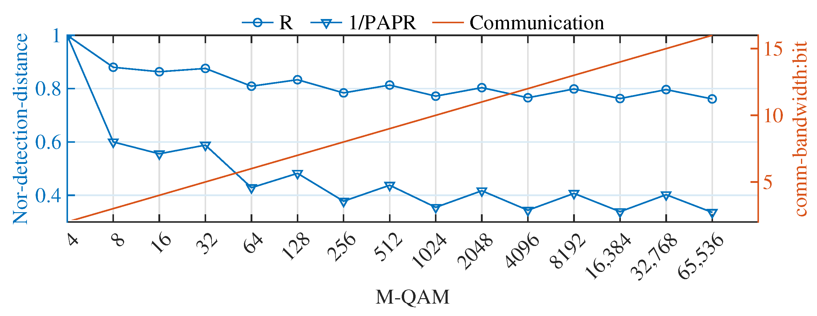
5.2.2. Analysis of Communication Rate

Building upon the traditional QAM-FH-MIMO DFRC implementation of frequency, phase, and amplitude modulation, the proposed CRM introduces a new dimension of constellation diagram rotation. This innovative approach significantly enhances the communication bandwidth. A comparison of the communication data rates under different information embedding modulation methods in FH-MIMO DFRC, as shown in

Table 4. Comparison of communication rates for different information embedding methods.

Modulation Method	Data Rate (bit/s)
FHCS-MIMO	$f_{\mathrm{p}}H⌊{\log }_2\left(C_K^M\right)⌋$
QAM-FHCS-MIMO	$f_{\mathrm{p}}H\left(⌊{\log }_2\left(C_K^M\right)⌋+M{log}_2\mathcal{M}\right)$
CRM-QAM-FHCS-MIMO	$f_{\mathrm{p}}H\left(⌊{\log }_2\left(C_K^M\right)⌋+M{log}_2\mathcal{M}\right)+f_{\mathrm{p}}⌊Z{log}_{2}Y⌋$
OFDM	$f_{\mathrm{p}}KH{log}_2\mathcal{M}$

, revealed that the communication rate increases in an additive manner with an increase in the dimensions of information embedding. For comparison, the communication rate of OFDM modulation under the same hardware constraints is also provided.

Assuming the number of pulse frequency points $K=10$, the range of the number of transmit antennas was $M=3\sim 8$, the number of sub-hops contained in the radar pulse was $H=5\sim 20$, the CRM modulation order was set to 4, the CRM symbol sample size was $L=2$, and 4QAM ($\mathcal{M}=4$) modulation was used. The number of bits that can be carried by each pulse under the different information embedding methods corresponding to Table 4 is shown in Figure 14. It can be observed that FHCS carried the fewest bits, and the introduction of QAM led to a rapid increase in communication bandwidth. Furthermore, the introduction of CRM further enhanced the communication bandwidth. In comparison with traditional OFDM signals, OFDM has an advantage in communication rate when the number of transmit antennas M is small. However, when M increases ($M>4$), both FHCS-MIMO DFRC with QAM and CRM surpass OFDM in terms of communication bandwidth.

6. CRM DFRC Communication Modulation Experiment

To demonstrate the practical feasibility of the CRM-based information embedding strategy, we conducted an indoor communication experiment using two SDR platforms, as illustrated in Figure 15. SDR1, based on the Xilinx Zynq ZC706, serves as the transmitter, while SDR2, using the ZedBoard, acts as the receiver. The transmitter operates with an output power of approximately $-5$ dBm, and the receiver applies a channel gain of around 40 dB. Both the transmitting and receiving antennas are omnidirectional, with a gain of roughly 8 dBi. Each SDR platform connects to a computer via Ethernet, with both platforms compatible with MATLAB [39].

Based on the simulation parameters in Table 2, the communication experiment utilized two transmission channels, i.e., $M=2$, while the reception used only one channel. Considering the need for channel parameter estimation, the waveform structure proposed in [32] was applied, where the first two sub-hops of each pulse were dedicated to channel estimation. Therefore, we set $H=10$, $H_{\mathrm{c}}=8$, and the number of QAM symbols in each CRM symbol as $L=16$. The CRM rotation angles include four distinct states, with their values and other essential parameters consistent with those listed in Table 2.

Figure 16a shows the time-domain signal for a single echo based on CRM-QAM-FHCS-MIMO DFRC. The varying frequency and amplitude across sub-hops due to QAM modulation are clearly visible. Figure 16b illustrates the time-domain waveform over 10,240 PRT echoes. The first two sub-hops of each pulse showed regularity as they were reserved for channel parameter estimation and did not carry CRM information, which is in line with the waveform design in [32]. The observed shift in the echo envelope, as shown in Figure 16b, was due to a significant Carrier Frequency Offset (CFO) between the transmit and receive systems.

Based on the error estimation theory from [32], after completing channel error estimation and compensation, the CRM-16QAM constellation diagram was created, as shown in Figure 17a. Since CRM used four rotation angles in the experiment, the diagram displays the superimposed 16QAM constellations under these four angles. After CRM demodulation, the 16QAM constellation, as shown in Figure 17b, was very close to the ideal, enabling accurate demodulation of the QAM symbols. Similarly, by keeping the four CRM rotation angles fixed and switching from 16QAM to 64QAM (where each CRM symbol still contains 16 QAM symbols), the pre- and post-demodulation CRM-64QAM constellation diagrams were constructed, as shown in Figure 17c,d. The 64QAM constellation was fully recovered after CRM demodulation.

The CRM demodulation results and theoretical predictions are presented in Figure 18. In this figure, “CRM_out” refers to the actual demodulated CRM code from the test, while “CRM_set” is the CRM code set at the transmitter. It is clear that the test results matched the transmitted codes exactly, validating the accuracy of the proposed modulation scheme.

7. Conclusions

This study proposes a method to enhance the communication bandwidth of the FH-MIMO DFRC system by utilizing CRM. Without increasing the system bandwidth or incurring additional overhead, this method significantly improves the communication bandwidth. The main achievements are as follows.

-

Systematically derived the principle of CRM information embedding, proposed a fast demodulation method based on constellation diagram folding and a demodulation method using the traditional least squares method, and compared their computational complexities and performance differences;

-

Analyzed the impact of the proposed method on radar performance from two perspectives: detection capability and ambiguity function performance. System simulation experiments demonstrated that the impact of CRM on radar performance is negligible;

-

Evaluated the theoretical performance of the proposed demodulation methods using BER curves. Simulation analyses confirmed that the method has a minimal impact on the demodulation performance in other dimensions;

-

Tested the CRM modulation and demodulation performance on an SDR experimental platform, verifying the feasibility of the proposed method;

-

Through simulation analyses and experimental validations, analyzed the CRM demodulation performance under different modulation orders, confirming the reliability of the proposed method.

The results indicate that this method can effectively increase the communication data transmission rate while maintaining radar detection performance, thus providing an effective technical approach to address the issue of scarce spectrum resources.

References

1. Wang, X.; Fei, Z.; Zhang, J.A.; Huang, J.; Yuan, J. Constrained Utility Maximization in Dual-Functional Radar-Communication Multi-UAV Networks. IEEE Trans. Commun. 2021, 69, 2660–2672. [Google Scholar] [CrossRef]
2. Wymeersch, H.; Seco-Granados, G.; Destino, G.; Dardari, D.; Tufvesson, F. 5G mmWave positioning for vehicular networks. IEEE Wirel. Commun. 2017, 24, 80–86. [Google Scholar] [CrossRef]
3. Yang, C.; Shao, H.R. WiFi-based indoor positioning. IEEE Commun. Mag. 2015, 53, 150–157. [Google Scholar] [CrossRef]
4. Liu, R.; Li, M.; Liu, Q.; Swindlehurst, A.L. Joint waveform and filter designs for STAP-SLP-based MIMO-DFRC systems. IEEE J. Sel. Areas Commun. 2022, 40, 1918–1931. [Google Scholar] [CrossRef]
5. Chen, L.; Qin, X.; Chen, Y.; Zhao, N. Joint waveform and clustering design for coordinated multi-point DFRC systems. IEEE Trans. Commun. 2023, 71, 1323–1335. [Google Scholar] [CrossRef]
6. Wu, K.; Zhang, J.A.; Huang, X.; Guo, Y.J.; Yuan, J. Reliable Frequency-Hopping MIMO Radar-Based Communications with Multi-Antenna Receiver. IEEE Trans. Commun. 2021, 69, 5502–5513. [Google Scholar] [CrossRef]
7. Hassanien, A.; Amin, M.G.; Aboutanios, E.; Himed, B. Dual-Function Radar Communication Systems: A Solution to the Spectrum Congestion Problem. IEEE Signal Process. Mag. 2019, 36, 115–126. [Google Scholar] [CrossRef]
8. Hassanien, A.; Amin, M.G.; Zhang, Y.D.; Ahmad, F. Dual-Function Radar-Communications: Information Embedding Using Sidelobe Control and Waveform Diversity. IEEE Trans. Signal Process. 2016, 64, 2168–2181. [Google Scholar] [CrossRef]
9. Wang, X.; Hassanien, A.; Amin, M.G. Dual-Function MIMO Radar Communications System Design Via Sparse Array Optimization. IEEE Trans. Aerosp. Electron. Syst. 2019, 55, 1213–1226. [Google Scholar] [CrossRef]
10. Tedesso, T.W.; Romero, R. Code shift keying based joint radar and communications for EMCON applications. Digit. Signal Process. 2018, 80, 48–56. [Google Scholar] [CrossRef]
11. Hassanien, A.; Aboutanios, E.; Amin, M.G.; Fabrizio, G.A. A dual-function MIMO radar-communication system via waveform permutation. Digit. Signal Process. 2018, 83, 118–128. [Google Scholar] [CrossRef]
12. Wu, K.; Zhang, J.A.; Huang, X.; Guo, Y.J. Frequency-hopping MIMO radar-based communications: An overview. IEEE Aerosp. Electron. Syst. Mag. 2021, 37, 42–54. [Google Scholar] [CrossRef]
13. Wang, X.; Hassanien, A. Phase Modulated Communications Embedded in Correlated FH-MIMO Radar Waveforms. In Proceedings of the 2020 IEEE Radar Conference (RadarConf20), Florence, Italy, 21–25 September 2020; pp. 1–6. [Google Scholar]
14. Eedara, I.P.; Amin, M.G.; Hassanien, A. Analysis of Communication Symbol Embedding in FH MIMO Radar Platforms. In Proceedings of the 2019 IEEE Radar Conference (RadarConf), Boston, MA, USA, 22–26 April 2019; pp. 1–6. [Google Scholar]
15. Eedara, I.P.; Amin, M.G.; Hassanien, A. Controlling Clutter Modulation in Frequency Hopping MIMO Dual-Function Radar Communication Systems. In Proceedings of the 2020 IEEE International Radar Conference (RADAR), Washington, DC, USA, 28–30 April 2020; pp. 466–471. [Google Scholar]
16. Yao, X.; Yang, Z.; Qiu, H.; Yu, X.; Cui, G.; Qi, H. DFRC signal design with hybrid index modulation. IEEE Sensors J. 2024, 24, 20855–20867. [Google Scholar] [CrossRef]
17. Ma, D.; Shlezinger, N.; Huang, T.; Shavit, Y.; Namer, M.; Liu, Y.; Eldar, Y.C. Spatial modulation for joint radar-communications systems: Design, analysis, and hardware prototype. IEEE Trans. Veh. Technol. 2021, 70, 2283–2298. [Google Scholar] [CrossRef]
18. Baxter, W.; Aboutanios, E.; Hassanien, A. Joint radar and communications for frequency-hopped MIMO systems. IEEE Trans. Signal Process. 2022, 70, 729–742. [Google Scholar] [CrossRef]
19. Eedara, I.P.; Amin, M.G. Dual Function FH MIMO Radar System with DPSK Signal Embedding. In Proceedings of the 2019 27th European Signal Processing Conference (EUSIPCO), A Coruna, Spain, 2–6 September 2019; pp. 1–5. [Google Scholar]
20. Hassanien, A.; Himed, B.; Rigling, B.D. A Dual-Function MIMO Radar-Communications System Using Frequency-Hopping Waveforms. In Proceedings of the 2017 IEEE Radar Conference (RadarConf), Seattle, WA, USA, 8–12 May 2017; pp. 1721–1725. [Google Scholar]
21. Baxter, W.; Aboutanios, E.; Hassanien, A. Dual-Function MIMO Radar-Communications Via Frequency-Hopping Code Selection. In Proceedings of the 2018 52nd Asilomar Conference on Signals, Systems, and Computers, Pacific Grove, CA, USA, 28–31 October 2018; pp. 1126–1130. [Google Scholar]
22. Qiu, F.; Zhao, M.M.; Li, L.; Zhao, M.J. Improved information embedding for frequency hopping-based mimo dfrc system. IEEE Wirel. Commun. Lett. 2022, 12, 346–350. [Google Scholar] [CrossRef]
23. Castillo-Soria, F.; Cortez, J.; Gutiérrez, C.; Luna-Rivera, M.; Garcia-Barrientos, A. Extended quadrature spatial modulation for MIMO wireless communications. Phys. Commun. 2019, 32, 88–95. [Google Scholar] [CrossRef]
24. Wang, X.; Xu, J.; Hassanien, A.; Aboutanios, E. Joint Communications with FH-MIMO Radar Systems: An Extended Signaling Strategy. In Proceedings of the ICASSP 2021-2021 IEEE International Conference on Acoustics, Speech and Signal Processing (ICASSP), Toronto, ON, Canada, 6–11 June 2021; pp. 8253–8257. [Google Scholar]
25. Eedara, I.P.; Hassanien, A.; Amin, M.G.; Rigling, B.D. Ambiguity Function Analysis for Dual-Function Radar Communications Using PSK Signaling. In Proceedings of the 2018 52nd Asilomar Conference on Signals, Systems, and Computers, Pacific Grove, CA, USA, 28–31 October 2018; pp. 900–904. [Google Scholar]
26. Wu, K.; Zhang, J.A.; Huang, X.; Guo, Y.J.; Heath, R.W. Waveform Design and Accurate Channel Estimation for Frequency-Hopping MIMO Radar-Based Communications. IEEE Trans. Commun. 2021, 69, 1244–1258. [Google Scholar] [CrossRef]
27. Wu, K.; Andrew Zhang, J.; Huang, X.; Jay Guo, Y. Integrating Secure Communications into Frequency Hopping MIMO Radar with Improved Data Rate. IEEE Trans. Wirel. Commun. 2022, 21, 5392–5405. [Google Scholar] [CrossRef]
28. Dash, S.S.; Pythoud, F.; Baeuerle, B.; Josten, A.; Leuchtmann, P.; Hillerkuss, D.; Leuthold, J. Approaching the Shannon Limit Through Constellation Modulation. In Proceedings of the 2016 Optical Fiber Communications Conference and Exhibition (OFC), Anaheim, CA, USA, 20–24 March 2016; pp. 1–3. [Google Scholar]
29. Zhao, Y.; Hu, J.; Ding, Z.; Yang, K. Constellation Rotation Aided Modulation Design for the Multi-User SWIPT-NOMA. In Proceedings of the 2018 IEEE International Conference on Communications (ICC), Kansas City, MO, USA, 20–24 May 2018; pp. 1–6. [Google Scholar] [CrossRef]
30. Gozávez, D.; Giménez, J.J.; Gómez-Barquero, D.; Cardona, N. Rotated Constellations for Improved Time and Frequency Diversity in DVB-NGH. IEEE Trans. Broadcast. 2013, 59, 298–305. [Google Scholar] [CrossRef]
31. Tan, M.; Chen, W. Performance Comparison and Analysis of PSK and QAM. In Proceedings of the 2011 7th International Conference on Wireless Communications, Networking and Mobile Computing, Wuhan, China, 23–25 September 2011; pp. 1–4. [Google Scholar] [CrossRef]
32. Liu, J.; Wu, K.; Su, T.; Zhang, J.A. Practical frequency-hopping MIMO joint radar communications: Design and experiment. Digit. Commun. Networks 2024, 10, 1904–1914. [Google Scholar] [CrossRef]
33. Kang, E.W. Radar System Analysis, Design, and Simulation; Artech House: Washington, DC, USA, 2008. [Google Scholar]
34. Khan, W.; Qureshi, I.M.; Sultan, K. Ambiguity function of phased–MIMO radar with colocated antennas and its properties. IEEE Geosci. Remote Sens. Lett. 2013, 11, 1220–1224. [Google Scholar] [CrossRef]
35. Madisetti, V.K.; Young, I.T. The Digital Signal Processing Handbook-3 Volume Set; CRC Press: Boca Raton, FL, USA, 2018. [Google Scholar]
36. Chang, S.; Deng, Y.; Zhang, Y.; Zhao, Q.; Wang, R.; Zhang, K. An advanced scheme for range ambiguity suppression of spaceborne SAR based on blind source separation. IEEE Trans. Geosci. Remote Sens. 2022, 60, 5230112. [Google Scholar] [CrossRef]
37. Soriano, C.G. Review of Radar Detectors With Constant False Alarm Rate. Telemática 2020, 19, 78–90. [Google Scholar]
38. Tran, T.N.; Drab, K.; Daszykowski, M. Revised DBSCAN algorithm to cluster data with dense adjacent clusters. Chemom. Intell. Lab. Syst. 2013, 120, 92–96. [Google Scholar] [CrossRef]
39. MathWorks. Help Center. Available online: https://www.mathworks.com/help/pdf_doc/supportpkg/xilinxzynqbasedradio/xilinxzynqbasedradio_ug.pdf (accessed on 9 January 2024).
Figure 1. FH-MIMO waveform structure.
Remotesensing 17 01058 g001
Figure 2. CRM symbols.
Remotesensing 17 01058 g002
Figure 3. CRM-QAM-FH-MIMO principle.
Remotesensing 17 01058 g003
Figure 4. CRM symbol folding.
Remotesensing 17 01058 g004
Figure 5. The impact of the QAM modulation order M on detection range and communication bandwidth.
Remotesensing 17 01058 g005
Figure 6. Comparison of the ambiguity function performance at zero Doppler cut for different modulations.
Remotesensing 17 01058 g006
Figure 7. CRM-matched demodulation.
Remotesensing 17 01058 g007
Figure 8. Cost function distribution under different CRM orders.
Remotesensing 17 01058 g008
Figure 9. The relationship between the peak value of the cost function L peak ( θ ) and Y.
Remotesensing 17 01058 g009
Figure 10. BER curves of CRM−64QAM with different CRM symbol sample lengths (L).
Remotesensing 17 01058 g010
Figure 11. (a) Radar range−Doppler map (RDM); (b) radar detection results matched with simulated targets; and (c) side view of RDM amplitude with respect to range.
Remotesensing 17 01058 g011
Figure 12. The impact of different communication waveforms on radar detection performance.
Remotesensing 17 01058 g012
Figure 13. 64QAM -CRM BER curves. (a) BER curves of CRM demodulation under different L values. (b) BER curves of QAM demodulation under different L values based on CRM demodulation.
Remotesensing 17 01058 g013
Figure 14. Comparison of communication data rates under different information embedding modulation methods.
Remotesensing 17 01058 g014
Figure 15. Experiment scenario based on SDR platforms.
Remotesensing 17 01058 g015
Figure 16. CRM time-domain echo.
Remotesensing 17 01058 g016
Figure 17. CRM -16QAM test results. (a) CRM-16QAM constellation diagram; (b) 16QAM constellation diagram after CRM demodulation; (c) CRM-64QAM constellation diagram; and (d) 64QAM constellation diagram after CRM demodulation.
Remotesensing 17 01058 g017
Figure 18. CRM demodulation results.
Remotesensing 17 01058 g018