Abstract
As the climate continues to warm, the thawing of ice-rich permafrost leads to changes in the polygonal patterned ground (PPG) landscape, exhibiting an array of spatial heterogeneity in trough patterns, governing permafrost stability and hydrological and ecosystem dynamics. Developing accurate methods for detecting trough areas will allow us to better understand where the degradation of PPG occurs. The Geomorphon approach is proven to be a computationally efficient method that utilizes digital elevation models (DEMs) for terrain classification across multiple scales. In this study, we firstly evaluate the appliance of the Geomorphon algorithm in trough mapping in Prudhoe Bay (PB) in Alaska and the Wudaoliang region (WDL) on the central Qinghai–Tibet Plateau. We used the optimized DEM resolution, flatness threshold (t), and search radius (L) as input parameters for Geomorphon. The accuracy of trough recognition was evaluated against that of hand-digitized troughs and field measurements, using the mean intersection over union (mIOU) and the F1 Score. By setting a classification threshold, the troughs were detected where the Geomorphon values were larger than 6. The results show that (i) the lowest t value (0°) captured the microtopograhy of the troughs, while the larger L values paired with a DEM resolution of 50 cm diminished the impact of minor noise, improving the accuracy of trough detection; (ii) the optimized Geomorphon model produced trough maps with a high accuracy, achieving mIOU and F1 Scores of 0.89 and 0.90 in PB and 0.84 and 0.87 in WDL, respectively; and (iii) compared with the polygonal boundaries, the trough maps can derive the heterogeneous features to quantify the degradation of PPG. By comparing with the traditional terrain indices for trough classification, Geomorphon provides a direct classification of troughs, thus advancing the scientific reproducibility of comparisons in PB and WDL. This work provides a valuable method that may propel future pan-Arctic studies of trough mapping.
1. Introduction
In Northern Hemisphere permafrost environments, polygonal patterned ground (PPG) is a widely distributed periglacial landform, commonly known as ice wedge and sand wedge polygons [1]. These features evolve from thermal contraction cracks, formed by repeated freeze–thaw cycles and soil condition fluctuations, which fill with ice, sand, soil, or a combination thereof [2,3]. Over decades and centuries, these polygons interact and integrate to form PPG landscapes. Such formations are observed not only in circumarctic regions (such as European Russia, Alaska, Siberia, and northern Canada), Greenland, and Antarctica, but are also well developed in the high-altitude permafrost regions of the Qinghai–Tibet Plateau (QTP) [4,5,6].
In recent years, the increasing global temperature has led to the rapid degradation of PPG [7], evident at individual field sites [8,9] and through repeated InSAR mapping [10], which has identified degradation-induced subsidence. The melting of ice wedges results in the deepening and broadening of troughs at the meter scale, creating high spatial heterogeneity as the ground transitions from low-centered to high-centered polygons [11]. Rigorous field surveys have verified that troughs deepen and widen with PPG degradation [7]. Therefore, the variation in trough features is a critical indicator for monitoring PPG evolution. The decimeter-scale variability in troughs can drive significant heterogeneity in surface and soil hydrology [12,13], snow distribution [14], biogeochemical fluxes [15], ground temperatures [16,17], vegetation niches [18], permafrost stability [19,20], and carbon budget [21]. Deeper troughs can trap more snow, providing insulation and affecting the thermal conditions of the underlying active layer and ice wedge, which, in turn, influences the potential for further cracking and degradation of PPG [16,22]. The CryoGrid 3 permafrost modeling results also demonstrated that incorporating the heterogeneity of troughs can provide valuable insights into the pathways of PPG degradation [23,24,25]. In order to provide a more mechanistic explanation of why Geomorphon is well suited to identifying troughs, integrating permafrost thermal processes (e.g., thermal contraction cracking leading to trough formation) with trough heterogeneity will be a focus of our future work. This trough heterogeneity in width and depth was verified to be effective for qualifying the development of PPG degradation and permafrost thawing [26,27,28]. Therefore, high-resolution inventories of troughs are of significant hydrologic and ecologic interest in cold regions. This is especially crucial for understanding the complex and non-linear responses of permafrost landscapes to continued global warming on a landscape scale.
Given the importance of trough heterogeneity in restructuring surface hydrology and ecosystems, numerous studies have focused on high-precision trough mapping [29,30,31]. The average size of PPG typically ranges from 3 to 50 m, with mean trough widths of less than 5 m and mean depths of less than 1 m [1]. Consequently, high-resolution unmanned aerial vehicle (UAV) multi-source remote sensing data have made it possible to accurately extract troughs [32]. Based on this, various deep learning techniques, such as convolutional neural networks (CNNs), have been employed to delineate the boundaries of PPG in UAV optimal imagery and DEM data [33,34,35]. Overall, these studies mainly focus on delineating the polygon-level boundaries of PPG. However, considerable challenges remain in accurately extracting troughs, as opposed to delineating boundaries [31]. Witharana et al. [36] introduced an object-based image analysis method for extracting troughs using Worldview-2 satellite imagery. Braun and Andresen [28] delineated troughs using a CNN model. However, the classification accuracy of optical image-based trough extraction methods is often limited by the mixed pixels between troughs and centers, especially under similar vegetation coverage.
While remote sensing methods can extract trough areas with high accuracy, their reliance on surface reflectance might be misled by vegetation cover, shadows, and sensor resolution. A distinctive microtopography is exhibited in troughs with specific widths and depths. Therefore, high-resolution digital elevation model (DEM)-based landform classification methods offer promising opportunities for effectively identifying trough distributions [31]. For example, terrain analysis indices, such as the topographic wetness index (TWI) and Topographic Position Index (TPI), have proven effective in characterizing troughs in PPG landscapes [37]. However, these indices often have limitations in representing the complexity of landforms and may lack a direct classification of landform types [38,39]. Some existing statistical methods rely on local terrain derivatives like the slope, aspect, and curvature. However, these methods usually analyze these factors in isolation and do not consider the overall spatial pattern of the terrain.
The Geomorphon method for terrain classification represents a recent advancement at multiscales. This tool utilizes pattern recognition technology to identify the overall shape of the terrain [40]. The Geomorphon method can categorize 498 unique terrain types using simple ternary patterns to represent various forms of terrain. In practice, this method simplifies this classification into ten primary Geomorphons: fat, peak or summit, ridge, shoulder, spur, slope, hollow, footslope, valley, and pit or depression [41]. These categories effectively encompass all possible terrain forms within PPG landscapes [1]. Additionally, the Geomorphon method can determine local elementary forms at an optimal spatial scale. By adjusting the scale parameter, it can adapt to the complexity of the terrain and the user’s specific research question. Moreover, Geomorphon is less affected by noise in the elevation data compared to some other methods to reduce the impact of vegetation cover on landform classification. Thus, it has been widely used for geomorphological process and formation mechanism simulations [42] and landform recognition and classification [43,44] on both a large scale and meter scale. For example, Lou et al. [45] successfully applied the Geomorphon index to deep learning models for thermokarst terrain mapping; Cignetti et al. [46] proved this approach demonstrated an exceptional capability in identifying runoff-associated landforms; and Coria et al. [47] effectively employed this method for automated ecological site classification. However, up until now, this approach has mostly been used in microtopograhy clarification.
In this study, we utilized the Geomorphon algorithm to predict the trough distribution in two different permafrost environments. The objectives of this study were to (1) determine the optimal scale and parameters for the Geomorphon algorithm to accurately detect trough areas; (2) map the trough areas of PPG across both study areas using Geomorphon; and (3) assess the classification accuracy of the Geomorphon method for trough extraction by comparing it with hand-digitized trough and field measurements. This study aims to advance the development of high-resolution trough mapping, enhancing our ability to monitor and predict PPG evolution and its associated land–atmosphere carbon–climate interactions.
2. Materials and Methods
2.1. Study Area
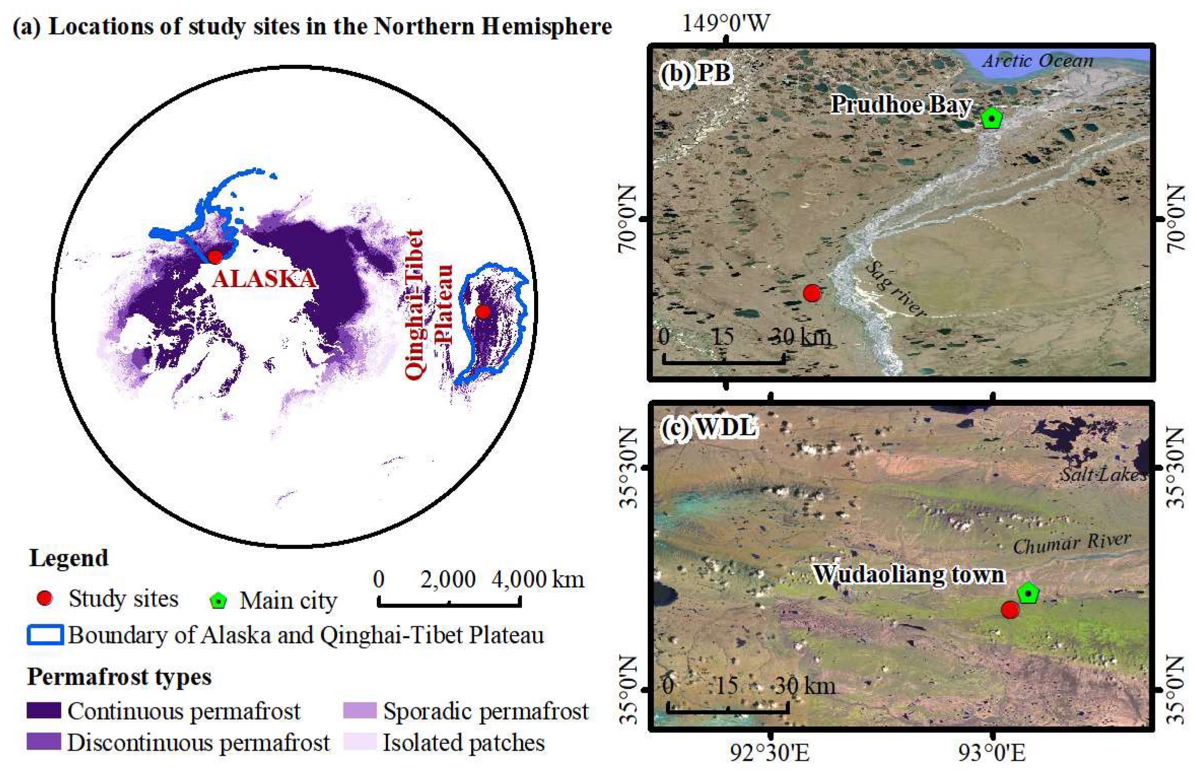
Two independent sites were selected to test the application of the Geomorphon method for extracting troughs (Figure 1). The first site was located approximately 40 km south of Prudhoe Bay (PB), Alaska, in the Arctic. The mesoscale topography is generally flat, with a slight dip (<4%) toward the northwest. Climatic data from the National Oceanic and Atmospheric Administration for the period 1981–2010 indicate a mean annual air temperature (MAAT) of −11.1 °C, a mean annual precipitation (MAP) of 102.6 mm, and an annual snowfall of 85.6 cm in PB (Table 1). EAR5 reanalysis data indicate that from 1957 to 2021, the MAAT in the region increased at a rate exceeding 5.3 °C/decade, and MAP increased at the rate of 3.22%/decade. Moreover, PB is underlain by cold continuous permafrost [48,49]. The freezing index (calculated by summing the daily deviations of ground temperatures below 0 °C) at PB averaged −4637.6 °C·day for the period between 1981 and 2010, whereas the thawing index (calculated by summing daily temperature deviations above 0 °C) averaged 593.3 °C·day.
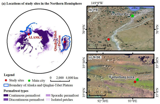
Figure 1.
The study sites: (a) locations of the two study sites in the Northern Hemisphere permafrost regions; (b) PB, south of Prudhoe Bay, Alaska, Arctic; (c) WDL, south of Wudaoliang town, near the source of the Yangtze River, central Qinghai–Tibet Plateau.

Table 1.
Summary of information regarding the two study sites.
The second site is located in the Wudaoliang region (WDL) of the central QTP. The mesoscale terrain is characterized by a basin, being relatively flat (slope < 5°). Climate records from the WDL station between 2010 and 2022 indicate a MAP of 314.3 mm and a MAAT of −4.82 °C (Table 1). Both MAAT and MAP showed a significant increasing trend, with rates of 4.6 °C/decade and 29.7 mm/decade, respectively. The freezing index at WDL averaged 1694 °C·day over the period from 1981 to 2013, whereas the thawing index averaged 1454.9 °C·day [50]. Additionally, this site is in a low-temperature continuous stage, with an active layer thickness of approximately 200 cm [51].
The sites were selected because (i) they present the typical PPG landscape in the Arctic and the QTP (Figure 2), respectively, and most importantly, (ii) these regions have traditionally been the focus of study for PPG mapping and permafrost thawing, allowing for comparison with previous studies.
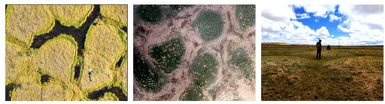
Figure 2.
Polygonal patterned ground at the two study sites: PB ((left), shown in UAV orthoimage) and WDL ((middle), shown in UAV orthoimage; (right), RTK field measurement for trough boundaries).
2.2. Drone DEM Data Acquisition and Pre-Processing
DEMs derived from airborne surveys conducted in PB and WDL were utilized for extracting troughs. For PB, airborne LiDAR data were downloaded from Abolt et al. [29]. The vertical accuracy of DEM was estimated to be 0.10 m. For WDL, DEM data were acquired using a FEIMA V300 fixed-wing drone (Feima Robotics Co. Ltd., Shenzhen, China) equipped with a Sony DSC-RX1RM2 digital RGB camera in April and August 2021. Before the flights, eight ground control points (GCPs) were uniformly arranged on the ground. The vertical and horizontal accuracy of the GCPs were measured using a Hi-Target iRTK2 differential GNSS device (Hi-Target Surveying Instrument Co. Ltd., Guangzhou, China), achieving approximately 0.01 m accuracy. The DSM imagery was produced using the Structure from Motion (SfM) workflow, implemented with Pix4D 4.7.0 software (Pix4D SA, Lausanne, Switzerland). Finally, 25 cm spatial resolution digital surface model (DSM) and orthomosaic imagery was generated.
To capture the fine-scale microtopography, DSM data in WDL needed to be converted into a digital elevation model (DEM). To generate a high-precision DEM, Cloth Simulation Filtering was used to remove non-ground points from the DSM data. Two-dimensional Delaunay Triangulation was used to generate TIN and fill holes left by point cloud filling. Then, the corresponding height value could be sampled from the triangular network for each DEM pixel one by one. DEM data at both sites were further refined by a Gaussian filter of 5 × 5 pixel kernel and a 1-pixel standard deviation (SD) to remove high-frequency noise using ArcGIS 10.0 software (ESRI, Redlands, CA, USA). The pre-processed DEM data were then processed into 25 cm, 50 cm, 100 cm, and 300 cm resolution, and subsequently projected to the World Geodetic System 1984 (WGS84) projection. The filtered and resampled DEMs were subsequently utilized to perform trough classification based on Geomorphon method.
2.3. Trough Classification Mapping Based on Geomorphon and Traditional Methods
To extract troughs of PPG, the Geomorphon algorithm was applied to all resolution DEMs using the ‘r.Geomorphon’ module in GRASS GIS 9.7.2 version (GRASS Development Team). Geomorphon utilizes the Local Binary Pattern (LBP) recognition approach, employing 8-tuple patterns from the visibility neighborhood [40]. The D∆L value is determined by the differences between the zenith and nadir angles, as described by Formula (1):
where and represent the nadir and zenith angles, respectively; D represents the eight compass directions; and t represents the flatness threshold.The results of the Geomorphon algorithm depend on two parameters: the search radius (L) and flatness threshold (t). A larger L is used for broader terrain classification, while a smaller L is suitable for local terrain identification. t represents the minimum difference between the zenith and nadir angles that is considered significantly different from the horizon. In this method, if the elevations of adjacent cells within a given line of sight are lower than that of the focus cell, the pixels are assigned a value of −1 (Figure 3). If there is no elevation change from the focus cell within the line of sight, the landform is considered flat, and the pixels are assigned a value of 0. Conversely, if the elevations of the surrounding cells are higher than that of the focus cell, the pixels are given a value of +1.
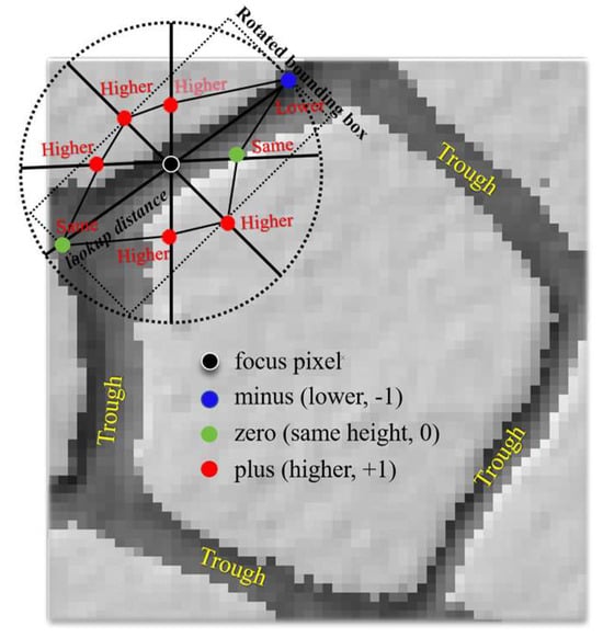
Figure 3.
Recognition of troughs in polygonal patterned ground based on the ‘r.geomorphon’ module GRASS GIS manual (revised from Jasiewicz & Stepinski [40]).
In this study, L values of 1, 5, 10, 20, 50, 100, 500, 1000, and 2000 pixels (ranging from 0.5 m to 1000 m), and t values of 0°, 1°, 3°, and 6°, were tested to evaluate their effectiveness in detecting troughs in PPG at both sites. Ten common Geomorphons were identified (see in Section 3.2), including fat, peak or summit, ridge, shoulder, spur, slope, hollow, footslope, valley, and pit or depression (the class labels for these Geomorphons are 1, 2, 3, 4, 5, 6, 7, 8, 9, and 10, respectively). The analysis was first conducted using topographic data at a 50 cm resolution and then repeated at 25 cm, 100 cm, and 300 cm resolutions. To extract the troughs of PPG, we further reclassified the 10 terrain landforms into two types based on a threshold: Class I (value ≤ 6) and Class II (value > 6) (see Section 3.2). Class II, which includes all pits or depressions, valleys, footslopes, and hollows, corresponded well to the distribution areas of troughs. However, the reclassified trough maps also included some noise, such as pits or depressions in the center or adjacent to rims. Consequently, we conducted a minority analysis using ENVI 5.6 software (Exelis, Boulder, Colorado) to clean up the majority of these noises. The post-classification maps were then converted into a shapefile. Hollows generated from raster to shapefile within trough areas were further filled using ArcGIS 10.0 software. The trough maps were further smoothed and high-precision trough maps were produced.
In order to assess the superiority of Geomorphon in trough extraction, this method was compared with polygon-level methods and three commonly used terrain indices, including a convolutional neural network (CNN) method, Topographic Position Index (TPI), System for Automated Geoscientific Analyses (SAGA) wetness index (SWI), and closed depressions. To operate CNN classification, the labels were designated as “Boundary” and “Not Boundary”, derived from a manually labeled UAV imagery. The training procedure was performed based on DEMs using the code written by Abolt et al. [29] in MATLAB (version R2017). The polygonal boundaries of PPG were generated and then compared with trough maps in this paper. Additionally, the TPI, SWI, and closed depressions were calculated based on DEMs using SAGA GIS v.2.12 [52]. TPI expressed the ratio of elevation difference between each cell to the mean elevation of a specified radius. According to the field survey and high-resolution UAV imagery, a radius of 200 m was selected. The trough classification also used a threshold approach. The setting of thresholds for three terrain indices refers to the manually digitized trough map. After acquiring the polygon boundaries and trough areas of PPG using these methods in both PB and WDL, we compared them with those generated using the Geomorphon method.
To identify the trough heterogeneity, two key geomorphological features—trough depth and trough width—were calculated based on the final generated trough maps. Observations at PB and WDL showed that a single trough could exhibit varying depths and widths over even short distances. Therefore, in this study, each multipart trough was divided into separate 1 m (length) segments, and the depth and width for each segment were measured individually. The trough widths and depths were then evaluated using the method proposed by Rettelbach et al. [53].
2.4. Accuracy Assessment
To evaluate the performance of the Geomorphon method, various error metrics were applied in the validation experiment. The mean intersection over union (mIOU) between the predicted and ground truth troughs was calculated using the formula:
where Ao represents the area of overlap between the predicted segmentation and the ground truth, and Au is the area of union between the predicted segmentation and the ground truth. An mIOU value greater than 0.5 is considered a “good” prediction, indicating successful delineation. In this study, mIOU values were calculated by comparing the predicted trough areas with those obtained from hand-digitization and filed measurements (as described in Section 2.2 and summarized in Table 2). Validation data were derived in two parts: the manual photointerpretation based on high-resolution UAV optical imagery, as well as ground truth measurements acquired using an RTK-GPS device (Figure 2). The optical imagery had resolutions of 0.2 m for PB and 0.25 m for WDL. Troughs were hand-digitized at scales ranging from 1:25 to 1:100 using ArcGIS software. Overall, a total of 1260 labeled troughs (approximately 20% of total polygons used to test the accuracy metrics of the Geomorphon algorithm) were collected. The validation dataset was randomly distributed across both study sites to represent various trough features and ensure the accuracy of the digitized data. To further enhance the accuracy of photointerpretation, we calibrated the hand-digitized troughs using ground truth data acquired from RTK-GPS at WDL, as well as field photos provided by the NWT Centre for Geomatics (www.geomatics.gov.nt.ca) and previous studies at the PB site.
Table 2.
Statistics of troughs in polygonal patterned ground based on degradation stages.
Additionally, the F1 score was used to measure the accuracy of the trough predictions, with a score of 1 indicating a perfect prediction. The metrics of correctness and completeness were also evaluated, where correctness reflects the proportion of predicted positives that are true positives, and completeness indicates the percentage of actual positives detected. Accurate predictions are indicated by all metric values being close to 1. The formulae for calculating these metrics are as follows:
Here, true positives (TP) represent the number of polygons correctly identified, false positives (FP) represent the number of polygons identified by the model that were not actually true, and false negatives (FN) represent the number of true polygons that were not detected by the model. We utilized the polygon boundaries generated by CNN method in Section 2.3 at PB and WDL to calculate the correctness, completeness, and F1 Score in Equations (3)–(5). The workflow of image preparation, trough mapping, accuracy assessment and further analysis was shown in Figure 4.
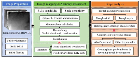
Figure 4.
Flowchart of datasets, processing methods, accuracy assessments, and graphical analyses conducted in this study.
3. Results
3.1. Influence of L, t Parameters, and DEM Resolution on Geomorphon Models
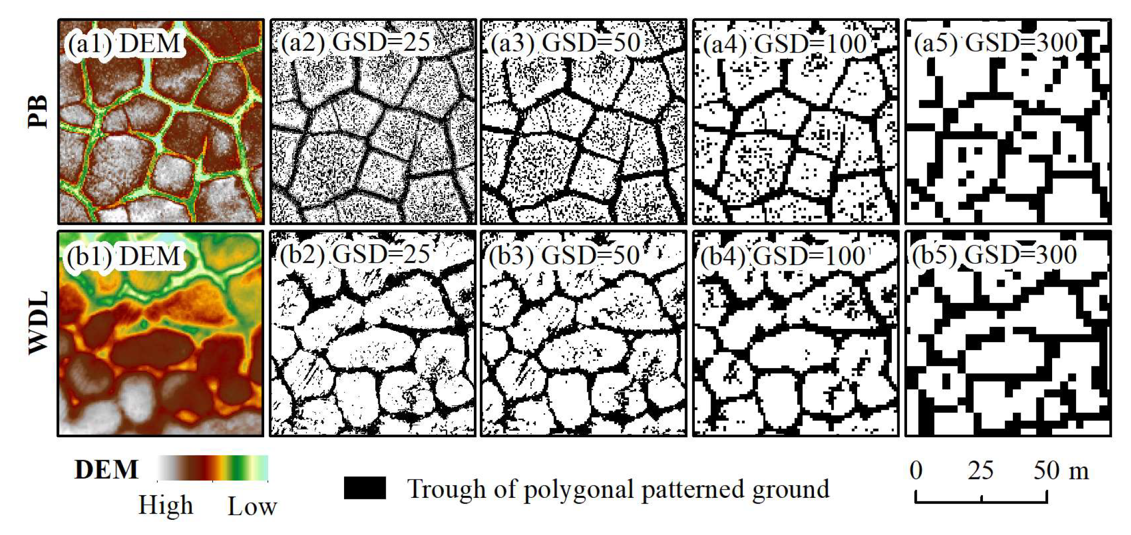
Permafrost and cryogenic processes can produce complexly polygonal landscapes. At the beginning, trough networks only a meter or two wide and less than a half-meter deep are established, while continued degradation will lead to variation in the trough width and depth. Therefore, to effectively detect the spatial heterogeneity of the trough areas, micro-landform classification for troughs using Geomorphon approach mapping must accurately capture the meter-scale topography variation. To evaluate how the DEM resolution influences the accuracy of trough identification, the DEM was resampled to 25 cm, 50 cm, 100 cm, and 300 cm. The Geomorphon algorithm was then applied, and the computational time was recorded for each resolution. Spatially, the impact of DEM resolutions on trough recognition is shown in Figure 5. When the delineation algorithm was repeated using the DEMs at 100 cm and 300 cm resolution, the delineation speeds increased somewhat, but the performance dropped significantly. This decline was more pronounced in trough areas with smaller widths, such as those less than 1 m. Additionally, the trough areas were successfully identified when using the DEM at 25 cm resolution, while larger fractions of fragmentary and false noise increased. Compared to 25 cm, 100 cm, and 300 cm resolutions, the completeness of trough recognition and computational efficiency showed the best performance at 50 cm resolution. Therefore, 50 cm DEM was used for the experiments conducted at PB and WDL, aligning with the conclusions of Abolt et al. [29].

Figure 5.
Performance of Geomorphon method on troughs at different resolutions: 25 cm, 50 cm, 100 cm, and 300 cm in PB ((a1)–(a5)) and WDL ((b1)–(b5)), respectively.
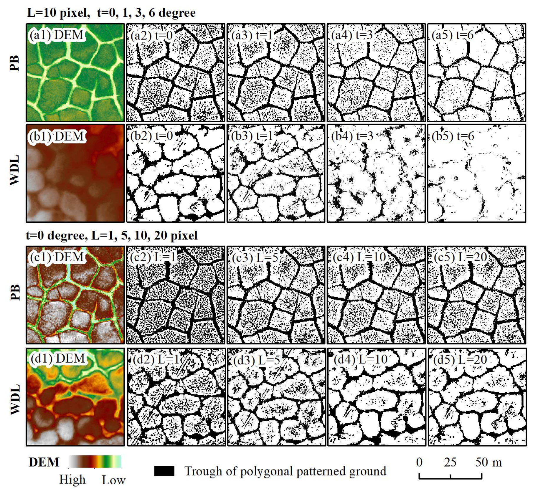
The sensitivity of the Geomorphon algorithm to the L and t values was investigated to determine their effects on the accuracy of trough pattern predictions (Figure 6). To determine the optimal L value, the t value was set to the default (0 degree). As L increased from 1 to 10, small pixels and noise details within the troughs gradually diminished, enhancing the completeness and connectivity of the troughs, especially when L reached 20 pixels. Smaller L values resulted in correct trough identification but also produced excessive redundant information. A comparison between the different L values at both PB and WDL indicated that 20 pixels (approximately 10 m) was optimal for trough extraction. Additionally, for t ranging from 0 to 6 degrees, higher values led to less detailed information, resulting in flatter maps and the loss of trough information, particularly at trough joints. Given the relatively flat topography of the two study areas (slope < 5°; maximum elevation relief of 3 m and 11 m at PB and WDL, respectively), a t value of 0 degrees was selected. Finally, after testing various configurations, an L value of 20 pixels and a t value of 0 degrees were selected for mapping the troughs.
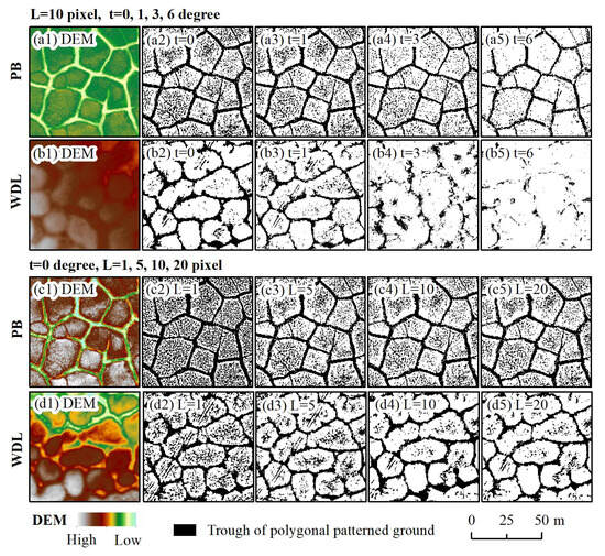
Figure 6.
Sensitivity analysis of L and t values on trough delineation. ((a2)–(a5)) and ((b2)–(b5)) represent t = 0 degrees, with L ranging from 1 to 5, 10, and 20 pixels at PB and WDL, respectively; ((c2)–(c5)) and ((d2)–(d5)) represent L = 10 pixels, with t ranging from 0 to 1, 3, and 6 degrees at PB and WDL, respectively.
3.2. Trough Recognition Using Geomorphon Method
Using the optimal parameters (L = 20 pixels, t = 0 degree, and DEM resolution = 50 cm) as input for the Geomorphon method, we generated the landform pattern recognition maps for PB and WDL, as shown in Figure 7(a2,b2). These maps effectively depict the distribution of troughs at both sites. To extract trough areas from these maps, a reclassification was necessary. We determined the reclassification threshold by randomly selecting two regions of interest, each measuring 80 m × 80 m, in both study areas. The histograms representing the Geomorphon values in these trough areas were then analyzed (Figure 7(a3,b3)), revealing statistically discernible troughs. This indicated that pixels with Geomorphon values greater than 6 accounted for 96.2% and 91.9% of the total trough areas at PB and WDL, respectively. Therefore, pixel values above 6 m were classified as troughs, while those below this threshold were assigned to a different class.
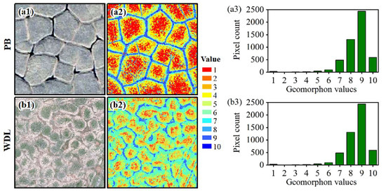
Figure 7.
Histograms of Geomorphon pixel values in trough areas at two sites: (a1) orthoimage at PB with a 0.2 m resolution; (a2) Geomorphon-based landform patterns at PB; (a3) histogram distribution of Geomorphon values in trough areas at PB. (b1)–(b3) correspond to WDL, with similar meanings.
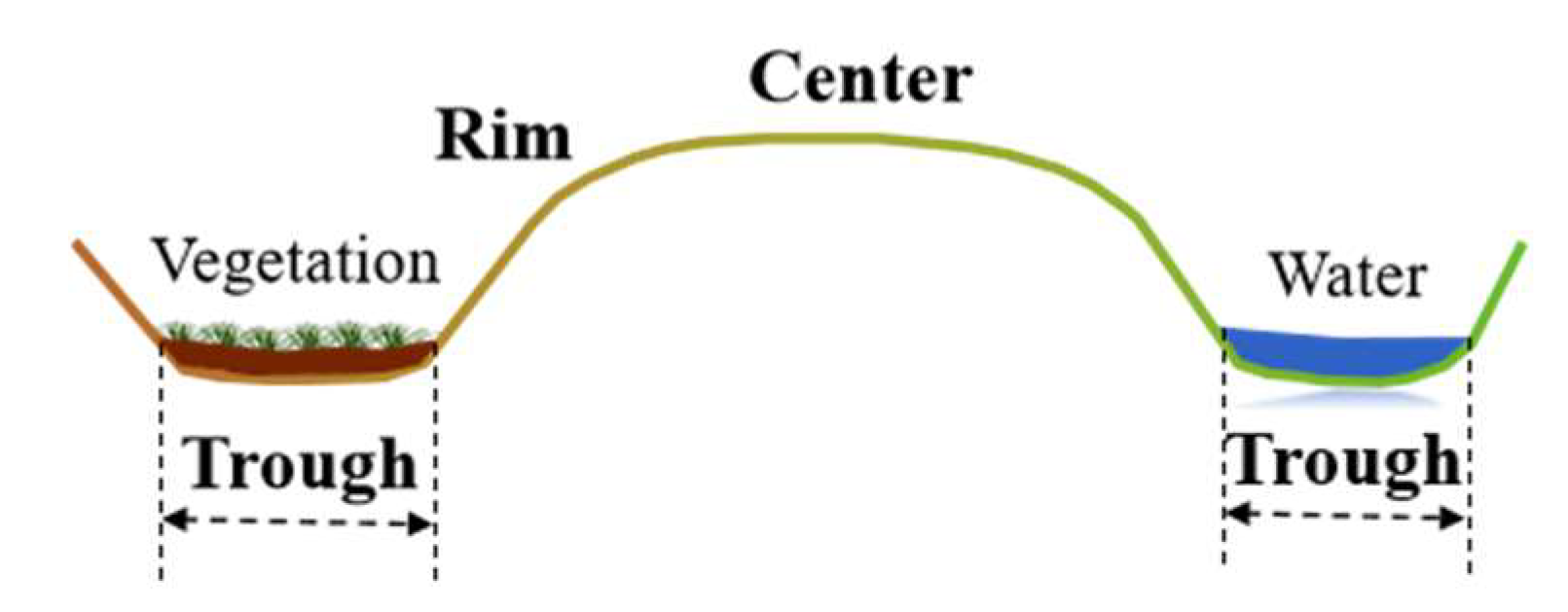
In the default labels for the Geomorphon outputs, values greater than 6 represent four landforms: hollow, footslope, valley, and pit or depression. The normal distribution paradigm for PPG troughs is shown in Figure 8. Notably, regardless of whether the troughs are water-filled or vegetated, they present the bottom regions of bowl-shaped landforms, excluding the rim slope regions. The trough area corresponded to Geomorphon landforms with values larger than 6. Therefore, the Geomorphon method can effectively depict the trough distribution across varying terrain conditions.
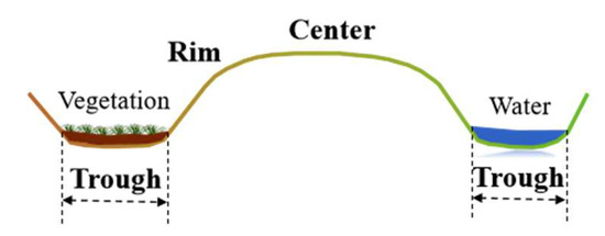
Figure 8.
Distribution paradigm for trough of high-centered polygon.
3.3. Trough Maps and Heterogeneous Trough Features
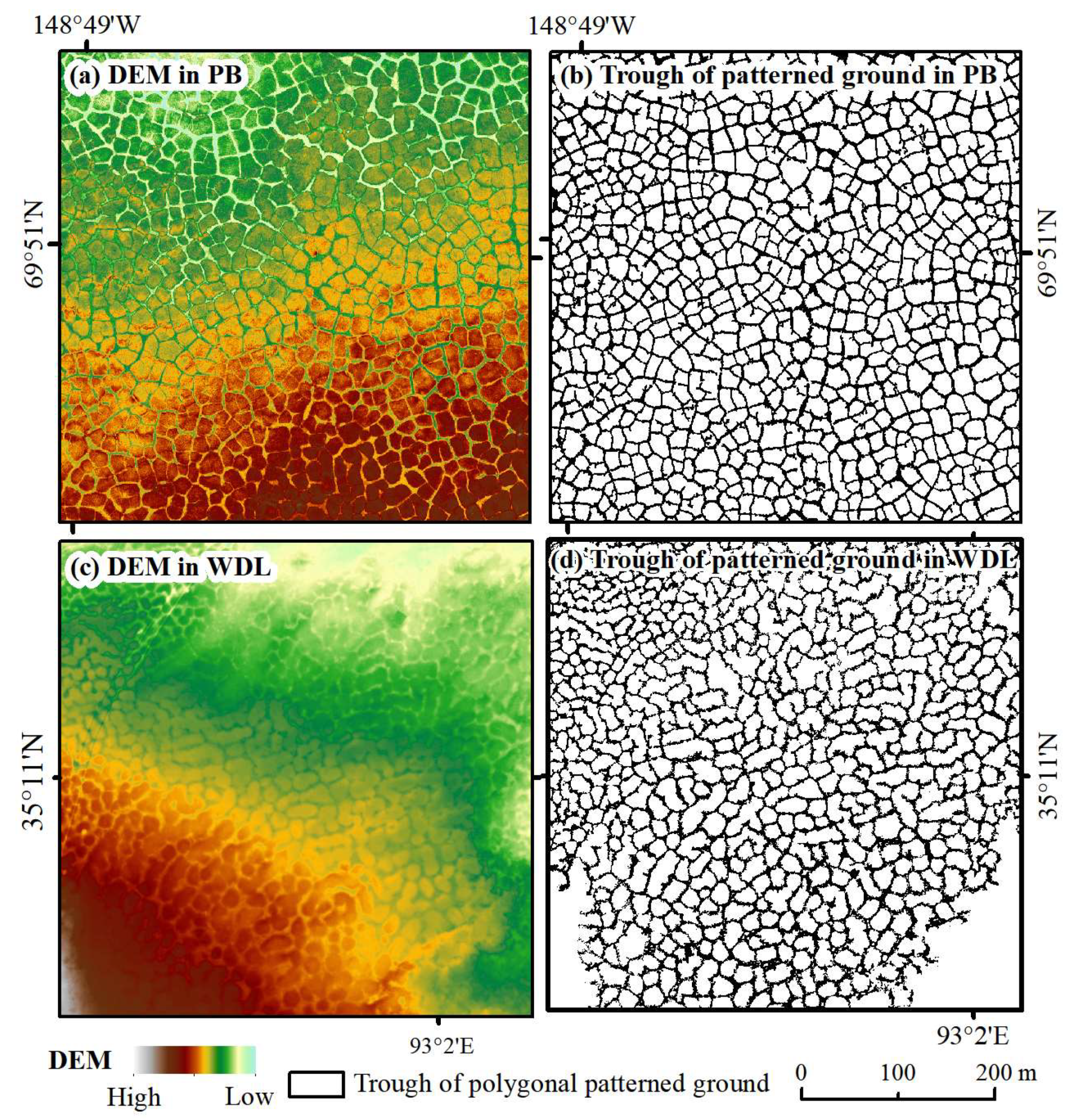
The extraction results of the troughs at the PB and WDL sites are illustrated in Figure 9. After quantifying the trough width and depth, the results indicate that at the PB site, the trough area covered approximately 0.18 km2, representing 18% of the total area of the PPG, with 3341 individual polygons identified. The trough width ranged from 0.5 to 7.8 m (mean = 3.7 m, SD = 1.6 m). Specifically, troughs less than 1 m wide accounted for 17.8% of the total, those between 1 and 2 m accounted for 30.83%, and those greater than 2 m accounted for 51.34%. Additionally, the trough depth ranged from 0.03 to 0.71 m (mean = 0.33 m, SD = 0.14 m), with depths greater than 0.05 m comprising 96.15% of the troughs. At the WDL site, the trough area was approximately 0.16 km2, accounting for 15.7% of the total study area, with 3218 individual polygons. The trough width ranged from 0.5 to 6.14 m (mean = 3.06, SD = 1.5). Specifically, troughs less than 1 m wide made up 11.75% of the total, those between 1 and 2 m accounted for 17.86%, and those greater than 2 m accounted for 70.37%. Additionally, the trough depth ranged from 0.01 to 1.09 m (mean = 0.49 m, SD = 0.22 m), with depths greater than 0.05 m accounting for 96.4%. These findings suggest that both sites are predominantly characterized by high-centered polygons. The statistical results of the trough properties (Table 3) confirm significant spatial heterogeneity in the troughs, particularly in terms of the width and depth (p < 0.05).
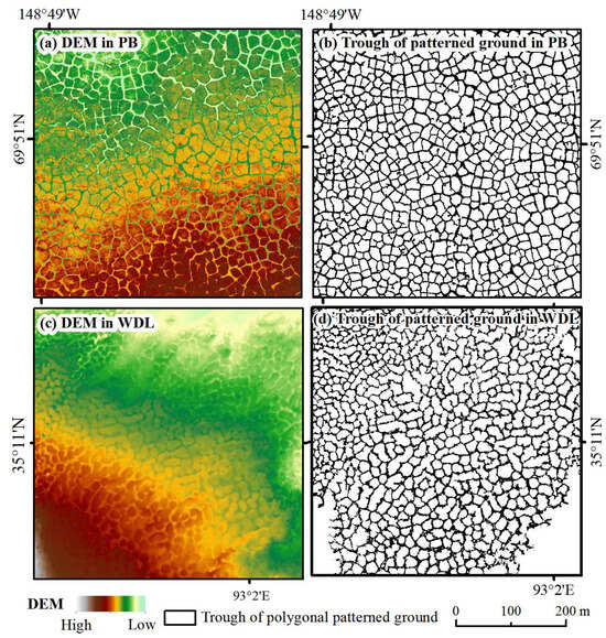
Figure 9.
Spatial distribution of troughs based on DEM data using the Geomorphon method at the two study areas: (a,b) PB and (c,d) WDL. Panels (a,b) display the DEM and trough patterns in PB, respectively, while panels (c,d) present the DEM and trough patterns in WDL.
Table 3.
Ratio (%) of troughs with heterogeneous properties to total troughs at each site.
3.4. Accuracy Assessment for Trough Extraction
To evaluate the effectiveness of the Geomorphon method for delineating troughs, we randomly selected 1260 ground truth and hand-digitized troughs (20% of the total polygons) and used metrics such as the mIOU, correctness, completeness, and F1 Score to assess the performance. The results are summarized in Table 4. Overall, the mIOU values reached 0.89 and 0.84 at PB and WDL, and the F1 Score varied between 0.87 and 0.90, respectively, indicating strong agreement between ground truth. To further assess the accuracy, we categorized the troughs into three classes, following the method proposed by Braun and Andresen [28]: undegraded (TW ≤ 1 m), degraded (1 m < TW ≤ 2 m), and stabilized (TW > 2 m). We calculated the mIOU values and F1 Score for each class at both PB and WDL sites (Table 4). The F1 Scores for all classes exceeded 0.82, with a maximum value of 0.93, indicating successful trough delineation in the permafrost environments of both PB and WDL. The Geomorphon method showed particularly strong performance for predicting the degraded and stabilized troughs (TW > 1 m), with the mIOU and F1 Scores ranging from 0.87 to 0.91 and 0.89 to 0.93, respectively. However, the Geomorphon method performed less effectively for the undegraded troughs. To investigate this, we further classified the troughs into high-centered polygons (TD > 0.05 m) and flat-centered polygons (TD ≤ 0.05 m) and calculated the corresponding F1 Scores and mIOU values. The analysis revealed that the Geomorphon method was less effective for delineating the flat-centered polygons, but it performed well for the high-centered polygons.
Table 4.
Accuracy assessment for trough delineation (n = 1260).
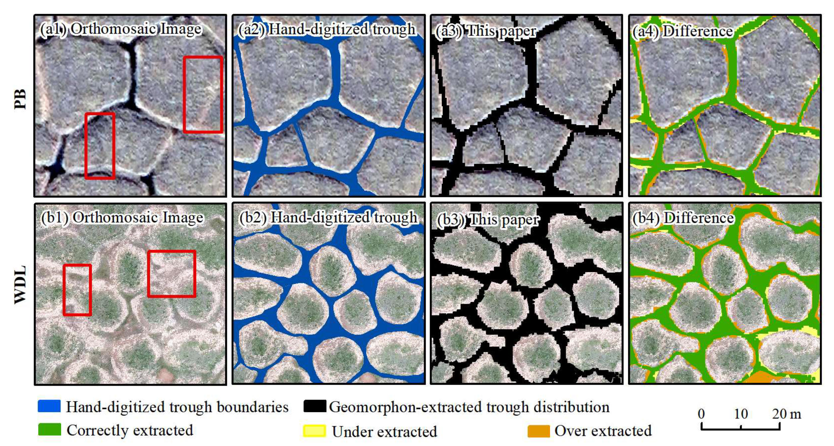
To further verify the spatial consistency between the predicted results and the manually delineated trough, we calculated their spatial differences at two sites (Figure 10). In the PB, the Geomorphon algorithm effectively predicted the patterns of troughs, including water-filled, moist, dry, or non-vegetated troughs. This was especially true for troughs without obvious spectral feature differences between the trough and the rim of the PPG (indicated by red rectangles in Figure 10(a1,b1)). The results were consistent at the WDL site as well. However, some over-extracted regions were observed along the trough boundaries (Figure 10(a4,b4)). Overall, the predicted trough closely matched the ground truth spatially. The DEM-based Geomorphon performed ideally in trough mapping to reveal the fine-scale heterogeneity of the troughs.

Figure 10.
Differences between predicted troughs and ground truth troughs. (a1) Orthomosaic imagery at PB; (a2) hand-digitized troughs based on UAV orthomosaic in (a1); (a3) trough areas from Geomorphon method in this paper; (a4) The spatial difference between Geomorphon based trough and hand-digitized trough. Panels ((b1)–(b4)) correspond to the same categories as ((a1)–(a4)) at the WDL site.
4. Discussions
4.1. Potential Influencing Factors Associated with Trough Classification Accuracy
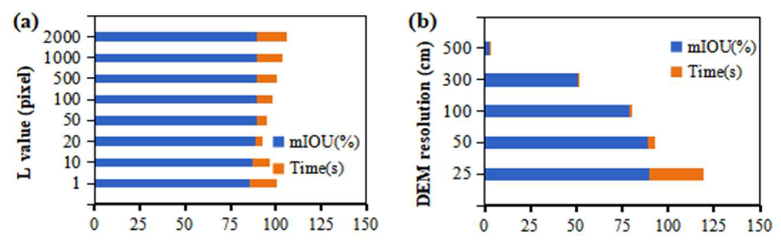
The distributions and characteristics of PPG have been proven to be scale-specific [23]. To determine the optimal scale for trough recognition, we examined how the L value and DEM resolution influence the classification accuracy and training speed in the Geomorphon model. The results, presented in Figure 11, show that the accuracy of trough delineation increased as the L value increased from 1 (minimum) to 20 pixels, accompanied by a noticeable decrease in the computation time (the Pearson correlation coefficient of R = −0.99) (Figure 11a). Generally, larger L values result in more accurate terrain classification outcomes, because smaller L values divide the landform into finer elements [54]. However, we observed that increasing the L value from 20 to 2000 pixels (default) did not significantly improve the accuracy, while computation time increased fourfold. This likely occurs because larger L values provide a broader and more generalized perspective on terrain classification. Given that the study areas each cover only 1 km2, the impact of L on the computation time was not substantial. However, for larger study areas, the increased DEM data volume can cause the computation time to rise exponentially. Therefore, we recommend that the range of L values should be determined based on the local terrain and the specific landform characteristics.

Figure 11.
Effects of different (a) L values and (b) DEM resolutions on the trough classification accuracy and training speed.
We also explored the scale effect of the DEM resolution on the classification accuracy of troughs; the results are presented in Figure 11b. The analysis of the accuracy and computation time across different DEM resolutions revealed a significant impact on trough extraction. As the DEM resolution decreased from 25 cm to 500 cm, the computation time also decreased, but the extraction accuracy of the troughs showed a decreasing trend. This decline in performance is attributed to the obscuration of finer polygonal boundaries at lower resolutions and the reduced amount of contextual information available from the neighborhood of any given pixel [55]. These factors diminish the algorithm’s ability to distinguish between polygonal troughs and other microtopographic depressions. Furthermore, while the highest classification accuracy for troughs was achieved at a 25 cm DEM resolution, surpassing even the performance at a 50 cm resolution, this resolution also resulted in longer computation times (30 s/km2). Therefore, a 50 cm resolution was deemed optimal for trough extraction, aligning with the conclusions of Abolt et al. [29].
Apart from the influence of Geomorphon parameters and DEM resolutions on trough classification, the acquisition time of the drone DEM cannot be neglected. Once snow filled the low-lying areas of the troughs [12,56], this resulted in the same elevation between the troughs and centers in the DEM imagery. The amount of troughs is likely be underestimated and the accuracy of trough classification will be unreliable [34]. Therefore, given the influence of snow cover on the DEM, the drone campaign was recommended to be conducted in a period of no snow cover.
4.2. Comparison to Polygon-Level Delineation Method
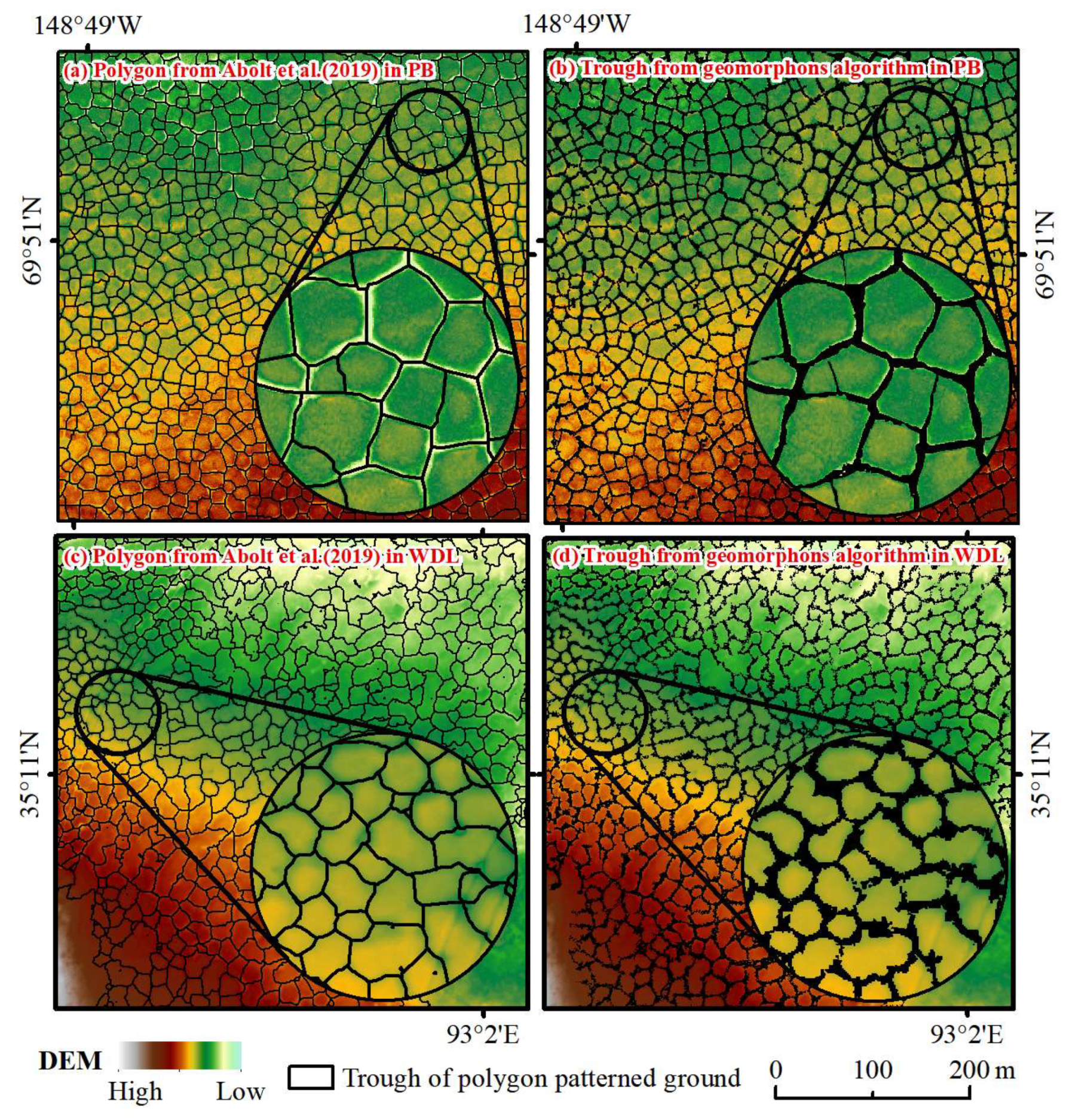
By comparing the trough maps derived from the CNN method [29] at PB and WDL, significant spatial differences in the troughs were observed visually on the meter scale (Figure 12). By using the semi-automatic Geomorphon algorithm, we detected the individual troughs with high performance across two sites at the meter-scale applied to a 0.5 m DEM. Over 3341 polygons were outlined, accounting for 18% of the total area of the PPG. Each had its own identification number and statistics, such as trough width and depth. In contrast, the CNN method provides well-defined polygon boundaries, while the trough features cannot be represented by a geomorphology map (Figure 12a,c).

Figure 12.
Differences between extracted troughs and boundaries: (a,c) Polygon boundaries determined using the method proposed by Abolt et al. [29]; (b,d) troughs determined using the Geomorphon method in this paper. Panels (a,b) correspond to work performed at the PB site, while panels (c,d) correspond to the WDL site.
Previous studies have also attempted to use deep learning or machine learning methods to identify trough areas based on optical images [36], relying on spectral differences between the trough and center. For example, Bhuiyan et al. [34] utilized the WorldView-2 imagery and mask R-CNN model to automatically map troughs across four different tundra landscapes, and the result showed that the mIoU values varied between 0.85 and 0.91; Witharana et al. [6] demonstrated that the overall accuracy of the CNN model’s predictions with respect to the fused products from multiple high-resolution commercial optical images was also less than 80%. When compared to the results obtained from the high-resolution optical images using other methods, our DEM-based trough detection method demonstrates a superior overall accuracy. The trough classification accuracy using optical imagery was influenced by mixed pixels between the troughs and center in the PPG, hindering the detection of troughs with minimal spectral differences. In conclusion, we strongly suggest that the DEM-based Geomorphon method has a greater value in extracting troughs and capturing their heterogeneous characteristics.
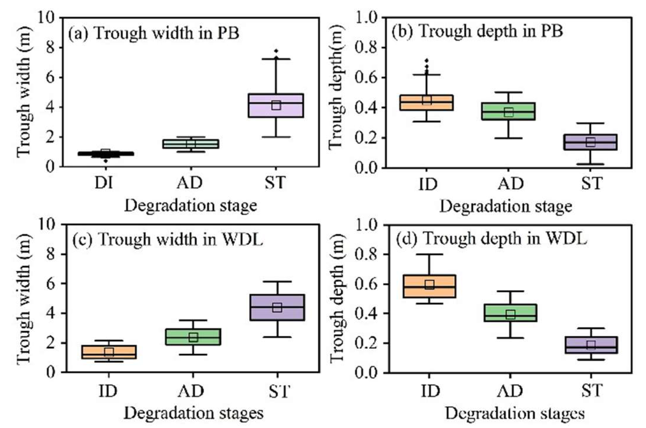
According to the study of Braun and Andresen [28], we further reclassified gradating PPG into three stages: initial degradation (ID), advanced degradation (AD), and stabilization (ST). The spatial variations in the trough properties are illustrated in Figure 13. The results reveal that the trough width and depth vary significantly between different degradation stages in both PB and WDL. The regression analysis showed that the significance level in all cases was <0.05. Each degradation stage exhibits discernibly different trough widths and depths. Overall, in the PB and WDL sites, the trough width increased as the degradation progressed. However, the trough depth decreased, which indicated that polygons were more likely to be shallow and flatter with accelerating climate warming. Therefore, high-resolution trough mapping is necessary for quantifying the dynamics of PPG evolution at a finer scale.
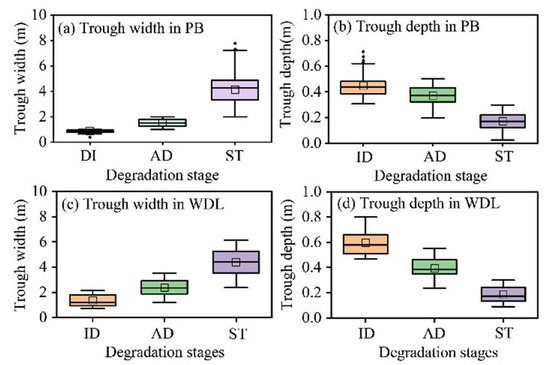
Figure 13.
Characteristics of troughs (based on classification map and elevation data): (a) trough width in PB; (b) trough depth in PB; (c) trough width in WDL; (d) trough depth in WDL; initial degradation (ID), advanced degradation (AD), and stabilization (ST).
4.3. Comparison to Other Terrain Classification Indices
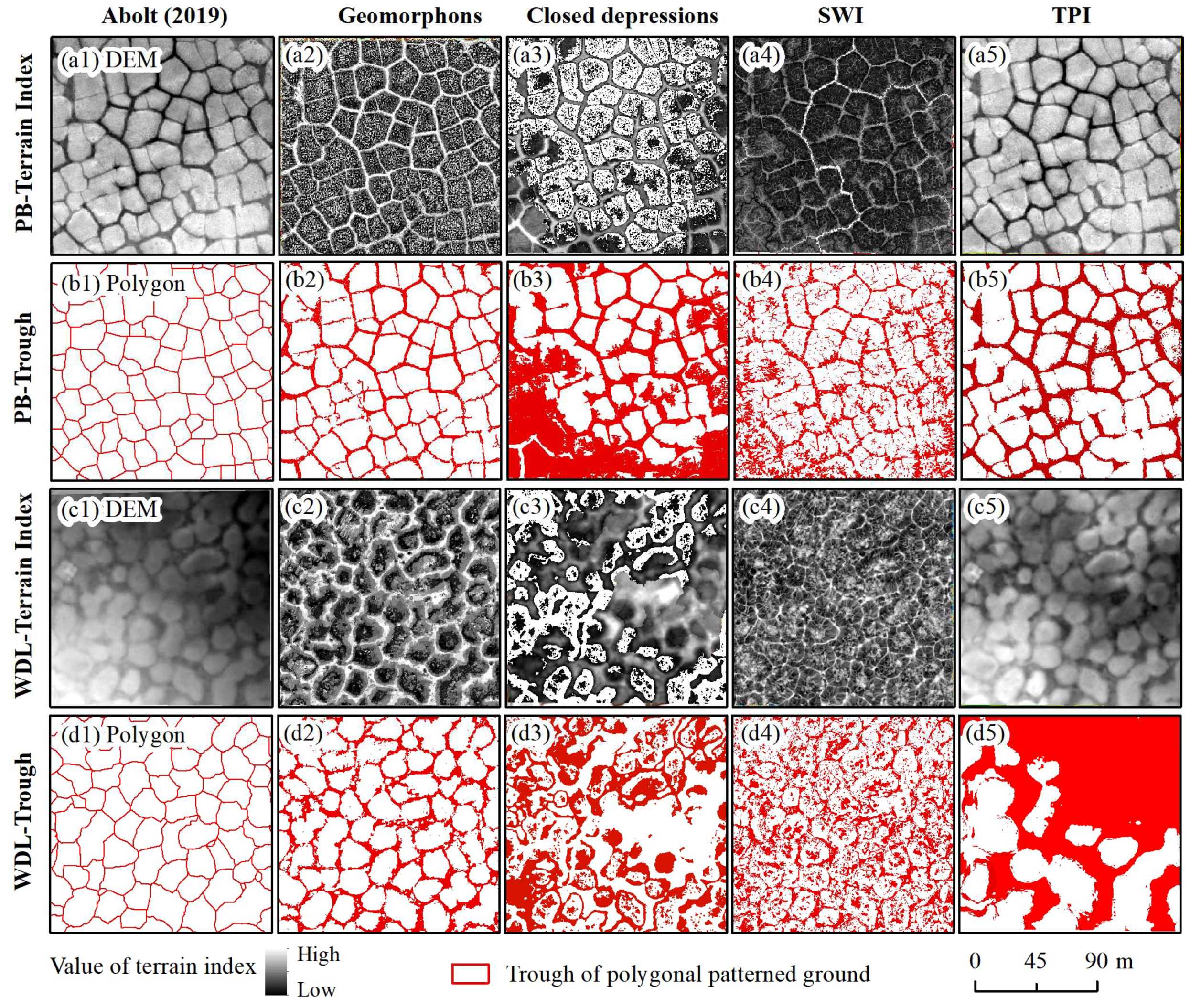
To assess the superiority of Geomorphon over other terrain classification indices in identifying PPG, the two most used terrain classification indices, including TPI and SWI, were calculated (Figure 14, Table 5). Previous studies have indicated that they were effective in identifying polygons in the Arctic tundra landscape [28,31]. Moreover, the closed depression index was also calculated because it can represent the area of depressions [16]. After comparison, the results indicated that, spatially, at the PB site, the origin raster maps of the SWI and TPI (Figure 14(a4,a5,c4,c5)) were effective at characterizing troughs in the flat regions We further reclassified the SWI and TPI maps into two classes according to the natural breaks to extract the trough maps (Figure 14(b4,b5)). This indicated that the TPI (completeness of 95.2%) performs better than the SWI (completeness of 51.8%), and both indices are more effective than the closed depression index (completeness of 43.4%). At the WDL site, the same terrain indices were calculated and reclassified using the same method. We found that the maps of the SWI and TPI aligned well with the spatial distribution of the troughs, compared to the closed depression index. These maps were also reclassified into two classes: trough and others (Figure 14(d3–d5)). The results show that the SWI (completeness of 41.7%) performs better than the TPI (completeness of 14.1%) and the closed depression index (completeness of 20.5%) in the slope regions (Figure 14(c4,c5)). Overall, in both PB and WDL, the original Geomorphon approach (Figure 14(a2,c2)), as well as the trough patterns (Figure 14(b2,d2)), match well with the ground truth (Figure 14(b1,d1)), with completeness of 98.5% and 98.0% in PB and WDL, respectively.
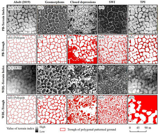
Figure 14.
Comparison of the Geomorphon method with closed depression index, SAGA wetness index (SWI), and Topographic Position Index (TPI) for identifying trough patterns [29]. ((a2)–(a5)) show the original raster maps of the four terrain indices at PB sites; ((b2)–(b5)) show troughs reclassified from corresponding terrain indices; ((c2)–(c5)) and ((d2)–(d5)) correspond to WDL, with similar meanings.
Table 5.
Comparison of the number and correctness ratio (%) of troughs classified by Geomorphon and other three terrain indices relative to in situ measurements.
It can be concluded that the Geomorphon can recognize microtopography variations and distinguish micro-landform units in both flat and slope regions. Although the recognized landform boundaries were mixed in landform superimposed areas (thermal erosion gullies, rivers, lakes, ponds and PPG), there was no difficulties when separating the “mixed types” from the classification results, because the size and shape of them were distinctive [1]. The recognition accuracy of the Geomorphon approach was not limited by the terrain complexity, land cover patterns, and climate condition, while it correlated with the quality of the DEM data and parameters of the Geomorphon model [43,44]. Therefore, we demonstrated that the Geomorphon method may exhibit a comparable accuracy in the regions with similar DEM and parameters to PB/WDL. In conclusion, as previously stated, the Geomorphon method outperforms the other three terrain indices in identifying troughs of PPG, demonstrating a better convergence and generalization ability.
The differences in trough identification among the terrain indices can be attributed to two main factors. Firstly, the TPI compares the elevation of each cell in a DEM to the mean elevation of a specified neighborhood around that cell, thereby identifying and categorizing the landform elements [57]. In contrast, the SWI implements a multiple-direction flow algorithm that iteratively modifies the catchment area based on the local slope and the flow accumulation of neighboring pixels. It quantifies the influence of topography on hydrological processes and can elucidate the general hydrological state [54]. Closed depressions on the land surface are identified by ‘filling’ a DEM and subtracting the filled model from the original DEM. Secondly, the flexibility and adaptability of these methods differ. The aforementioned terrain indices typically use a fixed-size neighborhood or object-based image analysis for landform classification, which can limit their ability to depict a comprehensive range of significant landform elements. In contrast, the Geomorphon technique, utilizing local ternary patterns—a concept adapted from image analysis—has proven effective in describing the texture of the land surface and delineating landform elements [58]. This method produces maps that provide a complete and satisfactory classification of landform elements at a relatively low computational cost. Moreover, unlike the fixed-size approaches, the Geomorphon method allows the size and shape of the neighborhood to adjust automatically according to the geometry of the local terrain. This flexibility makes the Geomorphon-based semi-automated classification method an effective approach for trough mapping.
4.4. Limitations and Future Research
PPG is an indicator of existing permafrost, and the formation and evolution of troughs in PPG can reflect the changes in permafrost to some extent [23,59]; terming the high-resolution mapping of trough patterns is of great importance. The performance of the Geomorphon method in extracting the distribution of troughs in both the Arctic and QTP permafrost environments was evaluated based on different aspects, such as predicting the trough patterns and addressing the spatial heterogeneity of the troughs. These evaluations were made by comparing the Geomorphon method with the commonly used CNN method, as well as terrain indexes, hand-digitized data, and ground truth measurements. Overall, the Geomorphon method demonstrated a good performance in trough extraction, achieving mIOU scores of 0.89 and 0.84 and F1 Scores of 0.90 and 0.87 for the PB and WDL sites, respectively. Compared with an object-based approach for trough mapping [36], the Geomorphon model improved the classification accuracy of the troughs; for example, the F1 score increased from 0.92 to 0.95. However, there are still limitations to this study.
By using the Geomorphon algorithm, the individual troughs of the polygons were identified with their own number and statistics. The total area and features of the troughs are likely an underestimate because the presence of PPG is not always evident on the ground surface. For example, the results for the undegraded troughs showed relatively lower mIOU and F1 scores. This is because of the flatter topography (<0.05 m) in the polygons, maintaining the detection of DEMs over the PPG or limited trough widths (<1 m). To increase the computational efficiency of the Geomorphon approach, the DEM resolution was resampled to 50 cm. When the 50 cm DEM imagery was set as the input data of the Geomorphon model, these shallow troughs or narrow troughs typically occupied fewer than two pixels at a 50 cm resolution. Additionally, under conditions where troughs are subject to interference from vegetation or other objects, or when troughs exhibit irregular geometric shapes, the pixels in the Geomorphon’s results may manifest as fragmented or discontinuous. These situations make them vulnerable in post-classification processes, such as smoothing, processing, and small patch removal. Recent advancements in deep learning for remote sensing classification, such as the CNN model [29,60] and Swin Transformer model [61,62,63,64], show greater potential in polygon or trough mapping. Future work should explore the potential of combining deep learning methods, such as the CNN model, with Geomorphon to enhance the performance of trough classification, and allow for applications over broader regions (potentially covering the entire Arctic and QTP).
Additionally, the overlapping accuracy (mIOU) of the trough maps was assessed against manually delineated trough boundaries. Hand-digitized troughs were derived by multiple trained operators through repeated digitization trials. The average positional discrepancies between the operators were quantified, yielding a mean deviation of ≤1 pixel, which aligns with the established tolerance error for manual digitization [65,66]. RTK measurements are highly accurate under clear spectral differences and texture features (e.g., pond-filled troughs), making them reliable for validation. However, their accuracy may decrease in areas with poor satellite visibility or signal interference. The variability in RTK data is generally low but can increase if measurement points are sparse or unevenly distributed. Overall, combining both methods helps balance their limitations: RTK provides a precise ground truth, while hand-digitized data offer continuous trough features [28]. To minimize variability, multiple measurements or cross-validation was used in this paper. However, due to the absence of measured data in the PB area, the reliability of the mIOU evaluation is somewhat compromised and requires improvement in future studies.
Furthermore, the fragmentation in Geomorphon outputs remains a significant limitation in the identification of flat-centered polygons. In the Geomorphon algorithm, landform types are identified based on the elevation relief of the surrounding areas. Minor elevation differences between the trough and the center of the PPG can lead to misidentifications of trough areas [67,68], sometimes confusing them with rims. To mitigate fragmentation in the Geomorphon method, we adjusted the search distance L and the flatness threshold t to minimize excessive fragmentation. Subsequently, we conducted strict post-classification processes to enhance the precision of trough mapping. Although it remains a significant challenge in the field, the area of the flat-centered polygons account for a relatively small proportion, and, thus, overall, the method produced promising classification accuracies. In future work, developing a hybrid model integrating object-oriented post-processing with deep learning will be necessary, thereby eliminating fragmented patches and optimizing boundary continuity [40]. Moreover, while two typical sites were selected to validate the suitability of Geomorphon for mapping troughs in flat- and high-centered polygons, the method’s effectiveness for low-centered PPG was not tested. Future studies should consider including more sites representing all types of PPG.
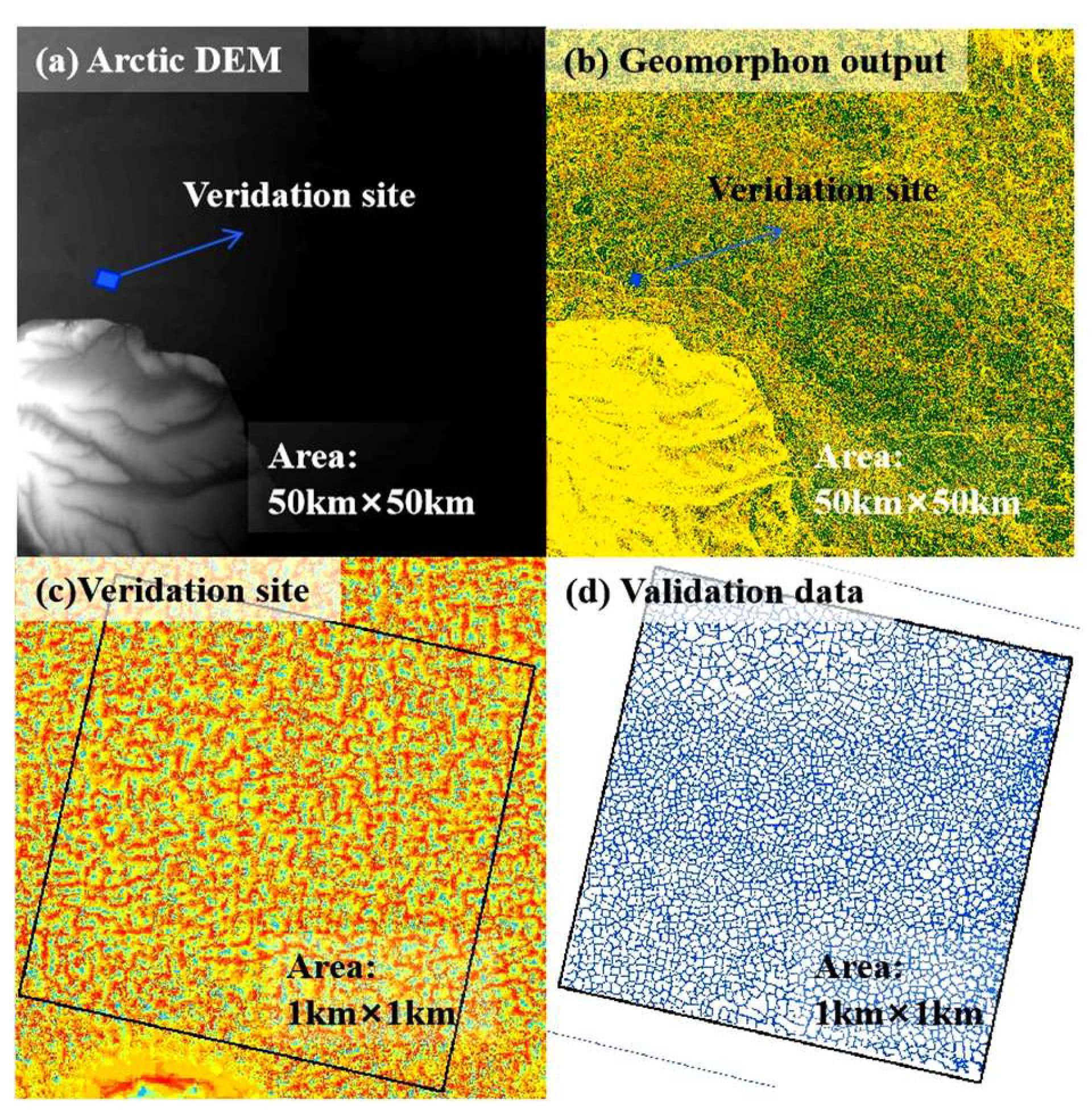
Moreover, detecting trough areas is inherently more challenging than identifying polygon boundaries but is crucial for understanding PPG in different degradation stages [69]. The variations in trough properties can significantly influence hydrological processes, the carbon and nitrogen content, soil microbial ecology, vegetation biomass, and soil water and heat dynamics in permafrost regions [70,71,72]. High-resolution DEM data are essential for the Geomorphon method [73]. However, acquiring such data on a large scale, especially in the QTP, is challenging. Considering the difficulty of UAV data acquisition, large-scale DEM products (e.g., ArcticDEM) have greater experimental value, allowing for applications over broader regions (potentially covering the entire Arctic). Merchant et al. [31] explored the combination of ArcticDEM (2 m) and SAR imagery (5 m) in a CNN model to map PPG. ArcticDEM was used to calculate the topographic wetness index (TWI), incorporating this into a CNN classification workflow. The results showed that the optimized CNN achieved a high classification accuracy (0.931 mean intersection over union; mIOU). Therefore, we agree that leveraging ArcticDEM could significantly broaden the applicability of our methodology across the Arctic region. In response to this, we conducted a preliminary evaluation of ArcticDEM’s compatibility in PB with the Geomorphon algorithm, covering an area of 50 km × 50 km; the result is shown in Figure 15. Compared with the polygon distribution from Abolt et al. [29] in Figure 15d, the results from Figure 15c indicate that while ArcticDEM marginally underestimates the trough complexity due to its coarser resolution, it effectively identifies PPG. Therefore, it can be demonstrated that ArcticDEM is suitable for supporting the Geomorphon algorithm and assessing its potential for large-scale trough mapping.
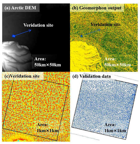
Figure 15.
Geomorphon outputs based on ArcticDEM data in PB: (a) ArcticDEM; (b) Geomorphon outputs (t = 0 degree, L = 20 pixel); (c) Geomorphon output in the validation site; and (d) validation data of polygon boundaries from Abolt et al. [29].
To address resolution limitations, a sensitivity analysis of the Geomorphon algorithm on a large scale should be conducted, improving the trough detection accuracy [74,75,76,77]. These modifications, coupled with ArcticDEM’s pan-Arctic coverage, suggest a strong potential for large-scale PPG mapping. Future research should explore combining the Geomorphon method with deep learning or multiscale segmentation methods using multi-source remote sensing imagery to achieve the high-resolution and large-scale mapping of PPG.
5. Conclusions
To advance high-precision trough mapping, we recommend a Geomorphon-based method using high-resolution DEM data. Overall, the results suggest that the trough modeling workflow exhibits substantial interoperability across different permafrost environments in PB in the Arctic and the WDL on the QTP, while achieving a promising classification accuracy. The main conclusions of this study are as follows:
- (1)
- We represents a novel technique that allows for high-precision trough mapping. We found that the Geomorphon model with a DEM resolution of 50 cm, t value of 0°, and L value of 20 produced the trough classification maps with the highest accuracy, achieving mIOU scores of 0.89 and 0.84 and F1 Scores of 0.90 and 0.87 for the PB and WDL sites, respectively.
- (2)
- At least 18.0% of the PPG landscape in PB and 15.7% of that in WDL is covered by troughs, respectively. The statistical analysis indicated that the trough width and depth exhibited significant spatial heterogeneity at the meter scale. In addition, this study highlights how the spatial variability in PPG degradation is associated with trough features, propelling future pan-Arctic studies of PPG evolution.
- (3)
- Compared to the polygon-level delineation method, the spatial heterogeneity in troughs produced by the Geomorphon method can quantify the degradation states of PPG. In addition, traditional terrain indices for trough classification have limitations in representing the complexity of landforms, while the Geomorphon approach provides a direct trough classification map. This shows improvements in the scientific reproducibility when compared with different permafrost environments in PB in the Arctic and the WDL on the QTP.
Author Contributions
Conceptualization, A.W. and T.W.; methodology, A.W. and J.C.; software, A.W.; validation, P.L., J.C. and A.W.; formal analysis, X.M.; investigation, A.W., P.L., X.Z. and J.S.; resources, T.W. and X.W.; data curation, A.W.; writing—original draft preparation, A.W.; writing—review and editing, D.W. and X.M.; visualization, A.W.; supervision, T.W.; project administration, T.W.; funding acquisition, T.W. and X.W. All authors have read and agreed to the published version of the manuscript.
Funding
This work was supported by the National Key Research and Development Program of China (2020YFA0608500 and 2022YFF0801903), the Gansu Provincial Science and Technology Program (22ZD6FA005), the Program of the State Key Laboratory of Cryospheric Science and Frozen Soil Engineering, CAS (No. CSFSE-TZ-2402), and the CAS “Light of West China” program (xbzg-zdsys-202304).
Data Availability Statement
The data will be made available on request.
Acknowledgments
The logistical support from the Cryosphere Research Station on the Qinghai–Tibet Plateau is especially appreciated.
Conflicts of Interest
The authors declare that they have no known competing financial interests or personal relationships that could have appeared to influence the work reported in this paper.
References
- French, H.M. The Periglacial Environment; John Wiley & Sons: Hoboken, NJ, USA, 2017. [Google Scholar]
- Romanovskij, N.N. Distribution of recently active ice and soil wedges in the USSR. In Field and Theory; University of British Columbia Press: Vancouver, BC, Canada, 1985; pp. 154–165. [Google Scholar] [CrossRef]
- Mackay, J.R.; Burn, C.R. The first 20 years (1978–1979 to 1998–1999) of ice-wedge growth at the Illisarvik experimental drained lake site, western Arctic coast, Canada. Can. J. Earth Sci. 2002, 39, 95–111. [Google Scholar] [CrossRef]
- Jin, H.; Vandenberghe, J.; Luo, D.; Harris, S.A.; He, R.; Chen, X.; Jin, X.; Wang, Q.; Zhang, Z.; Spektor, V.; et al. Quaternary Permafrost in China: Framework and Discussions. Quaternary 2020, 3, 32. [Google Scholar] [CrossRef]
- Karjalainen, O.; Luoto, M.; Aalto, J.; Etzelmüller, B.; Grosse, G.; Jones, B.M.; Lilleøren, K.S.; Hjort, J. High potential for loss of permafrost landforms in a changing climate. Environ. Res. Lett. 2020, 15, 104065. [Google Scholar] [CrossRef]
- Olefeldt, D.; Goswami, S.; Grosse, G.; Hayes, D.; Hugelius, G.; Kuhry, P.; McGuire, A.D.; Romanovsky, V.E.; Sannel, A.B.K.; Schuur, E.A.G.; et al. Circumpolar distribution and carbon storage of thermokarst landscapes. Nat. Comm. 2016, 7, 13043. [Google Scholar] [CrossRef]
- Lewkowicz, A.G.; Way, R.G. Extremes of summer climate trigger thousands of thermokarst landslides in a High Arctic environment. Nat. Comm. 2019, 10, 1329. [Google Scholar] [CrossRef]
- Walker, D.A.; Raynolds, M.K.; Kanevskiy, M.Z.; Shur, Y.S.; Romanovsky, V.E.; Jones, B.M.; Buchhorn, M.; Jorgenson, M.T.; Sibík, J.; Breen, A.L.; et al. Cumulative Impacts of a Gravel Road and Climate Change in an Ice-Wedge Polygon Landscape, Prudhoe Bay, AK. Arctic Sci. 2022, 8, 1040–1066. [Google Scholar] [CrossRef]
- Nitzbon, J.; Westermann, S.; Langer, M.; Martin, L.C.; Strauss, J.; Laboor, S.; Boike, J. Fast response of cold ice-rich permafrost in northeast Siberia to a warming climate. Nat. Commun. 2020, 11, 2201. [Google Scholar] [CrossRef]
- Deng, H.; Zhang, Z.; Wu, Y. Accelerated permafrost degradation in thermokarst landforms in Qilian Mountains from 2007 to 2020 observed by SBAS-InSAR. Ecol. Indic. 2024, 159, 111724. [Google Scholar] [CrossRef]
- Godin, E.; Fortier, D.; Lévesque, E. Nonlinear thermal and moisture response of ice-wedge polygons to permafrost disturbance increases heterogeneity of high Arctic wetland. Biogeosciences 2016, 13, 1439–1452. [Google Scholar] [CrossRef]
- Liljedahl, A.K.; Boike, J.; Daanen, R.P.; Fedorov, A.N.; Frost, G.V.; Grosse, G.; Hinzman, L.D.; Iijma, Y.; Jorgenson, J.C.; Matveyeva, N.; et al. Pan-Arctic ice-wedge degradation in warming permafrost and its influence on tundra hydrology. Nat. Geosci. 2016, 9, 312–318. [Google Scholar] [CrossRef]
- Speetjens, N.J.; Berghuijs, W.R.; Wagner, J.; Vonk, J.E. Degradation of ice-wedge polygons leads to increased fluxes of water and DOC. Sci. Total Environ. 2024, 920, 170931. [Google Scholar] [CrossRef] [PubMed]
- Mackay, J.R. Air temperature, snow cover, creep of frozen ground, and the time of ice-wedge cracking, western Arctic coast. Can. J. Earth Sci. 1993, 30, 1720–1729. [Google Scholar] [CrossRef]
- Jones, E.L.; Hodson, A.J.; Redeker, K.R.; Christiansen, H.H.; Thornton, S.F.; Rogers, J. Biogeochemistry of low- and high-centered ice-wedge polygons in wetlands in Svalbard. Permafr. Periglac. Process 2023, 34, 35–369. [Google Scholar] [CrossRef]
- Abolt, C.J.; Young, M.H.; Atchley, A.L.; Brown, C.J. CNN-watershed: A machine-learning based tool for delineation and measurement of ice wedge polygons in high-resolution digital elevation models. Zenodo Repos. 2018, 25, 237–245. [Google Scholar]
- Ward Jones, M.K.; Pollard, W.H.; Amyot, F. Impacts of degrading ice-wedges on ground temperatures in a high Arctic polar desert system. J. Geophys. Res-Earth. 2020, 125, e2019JF005173. [Google Scholar] [CrossRef]
- Higgins, S.I.; Conradi, T.; Muhoko, E. Shifts in vegetation activity of terrestrial ecosystems attributable to climate trends. Nat. Geosci. 2023, 16, 147–153. [Google Scholar] [CrossRef]
- Painter, S.L.; Coon, E.T.; Khattak, A.J.; Jastrow, J.D. Drying of tundra landscapes will limit subsidence-induced acceleration of permafrost thaw. Proc. Natl. Acad. Sci. USA 2023, 120, e2212171120. [Google Scholar] [CrossRef]
- O’Neill, H.B.; Wolfe, S.A.; Duchesne, C.; Parker, R.J. Effect of surficial geology mapping scale on modelled ground ice in Canadian Shield terrain. Cryosphere 2024, 18, 2979–2990. [Google Scholar] [CrossRef]
- Lara, M.J.; McGuire, A.D.; Euskirchen, E.S.; Genet, H.; Yi, S.; Rutter, R.; Iversen, C.; Sloan, V.; Wullschleger, S.D. Local-scale Arctic tundra heterogeneity affects regional-scale carbon dynamics. Nat. Commun. 2020, 11, 1–10. [Google Scholar] [CrossRef]
- Nitzbon, J.; Langer, M.; Martin, L.C.; Westermann, S.; Schneider von Deimling, T.; Boike, J. Effects of multi-scale heterogeneity on the simulated evolution of ice-rich permafrost lowlands under a warming climate. Cryosphere 2021, 15, 1399–1422. [Google Scholar] [CrossRef]
- Nitzbon, J.; Schneider von Deimling, T.; Aliyeva, M.; Chadburn, S.E.; Grosse, G.; Laboor, S.; Lee, H.; Lohmann, G.; Steinert, N.J.; Stuenzi, S.M.; et al. No respite from permafrost-thaw impacts in the absence of a global tipping point. Nat. Clim. Change 2024, 14, 573–585. [Google Scholar] [CrossRef]
- Liljedahl, A.K.; Witharana, C.; Manos, E. The capillaries of the Arctic tundra. Nat. Water 2024, 2, 611–614. [Google Scholar] [CrossRef]
- Chartrand, S.M.; Jellinek, A.M.; Kukko, A.; Galofre, A.G.; Osinski, G.R.; Hinnard, S. High Arctic channel incision modulated by climate change and the emergence of polygonal ground. Nat. Commun. 2023, 14, 5297. [Google Scholar] [CrossRef]
- Wainwright, H.M.; Oktem, R.; Dafflon, B.; Dengel, S.; Curtis, J.B.; Torn, M.S.; Cherry, J.; Hubbard, S.S. High-Resolution Spatio-Temporal Estimation of Net Ecosystem Exchange in Ice-Wedge Polygon Tundra Using In Situ Sensors and Remote Sensing Data. Land 2021, 10, 722. [Google Scholar] [CrossRef]
- Jorgenson, M.T.; Kanevskiy, M.Z.; Jorgenson, J.C.; Liljedahl, A.; Shur, Y.; Epstein, H.; Kent, K.; Griffin, C.G.; Daanen, R.; Boldenow, M.; et al. Rapid transformation of tundra ecosystems from ice-wedge degradation. Glob. Planet. Change 2022, 216, 103921. [Google Scholar] [CrossRef]
- Braun, K.N.; Andresen, C.G. Heterogeneity in ice-wedge permafrost degradation revealed across spatial scales. Remote Sens. Environ. 2024, 311, 114299. [Google Scholar] [CrossRef]
- Abolt, C.J.; Young, M.H.; Atchley, A.L.; Harp, D.R.; Coon, E.T. Feedbacks between surface deformation and permafrost degradation in ice wedge polygons, Arctic Coastal Plain, Alaska. J. Geophys. Res-Earth 2020, 125, e2019JF005349. [Google Scholar] [CrossRef]
- Witharana, C.; Bhuiyan, M.A.E.; Liljedahl, A.K.; Kanevskiy, M.; Epstein, H.E.; Jones, B.M.; Dannen, R.; Griffin, C.G.; Kent, K.; Ward Jones, M.K. Understanding the synergies of deep learning and data fusion of multispectral and panchromatic high resolution commercial satellite imagery for automated ice-wedge polygon detection. ISPRS J. Photogramm. Remote Sens. 2020, 170, 174–191. [Google Scholar] [CrossRef]
- Merchant, M.; Bourgeau-Chavez, L.; Mahdianpari, M.; Brisco, B.; Obadia, M.; DeVries, B.; Berg, A. Arctic ice-wedge landscape mapping by CNN using a fusion of Radarsat constellation Mission and ArcticDEM. Remote Sens. Environ. 2024, 304, 114052. [Google Scholar] [CrossRef]
- Nitze, I.; Grosse, G.; Jones, B.M.; Romanovsky, V.E.; Boike, J. Remote sensing quantifies widespread abundance of permafrost region disturbances across the Arctic and Subarctic. Nat. Commun. 2018, 9, 5423. [Google Scholar] [CrossRef]
- Zhang, W.; Witharana, C.; Liljedahl, A.K.; Kanevskiy, M. Deep Convolutional Neural Networks for Automated Characterization of Arctic Ice-Wedge Polygons in Very High Spatial Resolution Aerial Imagery. Remote Sens. 2018, 10, 1487. [Google Scholar] [CrossRef]
- Bhuiyan, M.A.E.; Witharana, C.; Liljedahl, A.K. Use of Very High Spatial Resolution Commercial Satellite Imagery and Deep Learning to Automatically Map Ice-Wedge Polygons across Tundra Vegetation Types. J. Imaging 2020, 6, 137. [Google Scholar] [CrossRef] [PubMed]
- Kartoziia, A. Assessment of the Ice Wedge Polygon Current State by Means of UAV Imagery Analysis (Samoylov Island, the Lena Delta). Remote Sens. 2019, 11, 1627. [Google Scholar] [CrossRef]
- Witharana, C.; Bhuiyan, M.A.E.; Liljedahl, A.K.; Kanevskiy, M.; Jorgenson, T.; Jones, B.M.; Daanen, R.; Epstein, H.E.; Griffin, C.G.; Kent, K.; et al. An Object-Based Approach for Mapping Tundra Ice-Wedge Polygon Troughs from Very High Spatial Resolution Optical Satellite Imagery. Remote Sens. 2021, 13, 558. [Google Scholar] [CrossRef]
- Riihimäki, H.; Kemppinen, J.; Kopecký, M.; Luoto, M. Topographic wetness index as a proxy for soil moisture: The importance of flow-routing algorithm and grid resolution. Water Resour. Res. 2021, 57, e2021WR029871. [Google Scholar] [CrossRef]
- Huang, L.; Luo, J.; Lin, Z.; Niu, F.; Liu, L. Using deep learning to map retrogressive thaw slumps in the Beiluhe region (Tibetan Plateau) from CubeSat images. Remote Sens. Environ. 2020, 237, 111534. [Google Scholar] [CrossRef]
- Shukla, T.; Tang, W.; Trettin, C.C.; Chen, G.; Chen, S.; Allan, C. Quantification of microtopography in natural ecosystems using close-range remote sensing. Remote Sens. 2023, 15, 2387. [Google Scholar] [CrossRef]
- Jasiewicz, J.; Stepinski, T.F. Geomorphon—A pattern recognition approach to classification and mapping of landforms. Geomorphology 2013, 182, 147–156. [Google Scholar] [CrossRef]
- Maxwell, A.E.; Shobe, C.M. Land-surface parameters for spatial predictive mapping and modeling. Earth-Sci. Rev. 2022, 226, 103944. [Google Scholar] [CrossRef]
- Ngunjiri, M.W.; Libohova, Z.; Owens, P.R.; Schulze, D.G. Landform pattern recognition and classification for predicting soil types of the Uasin Gishu Plateau, Kenya. Catena 2020, 188, 104390. [Google Scholar] [CrossRef]
- Flynn, T.; Rozanov., A.; Ellis, F.; de Clercq, W.; Clarke, C. Farm-scale soil patterns derived from automated terrain classification. Catena 2020, 185, 104311. [Google Scholar] [CrossRef]
- Gioia, D.; Danese, M.; Corrado, G.; Di Leo, P.; Minervino Amodio, A.; Schiattarella, M. Assessing the prediction accuracy of geomorphon-based automated landform classification: An example from the ionian coastal belt of southern Italy. ISPRS Int. J. Geo-Inf. 2021, 10, 725. [Google Scholar] [CrossRef]
- Lou, P.; Wu, T.; Yin, G.; Chen, J.; Zhu, X.; Wu, X.; Li, R.; Yang, S. A novel framework for multiple thermokarst hazards risk assessment and controlling environmental factors analysis on the Qinghai-Tibet Plateau. CATENA 2024, 246, 108367. [Google Scholar] [CrossRef]
- Cignetti, M.; Godone, D.; Ferrari Trecate, D.; Baldo, M. New Paradigms for Geomorphological Mapping: A Multi-Source Approach for Landscape Characterization. Remote Sens. 2025, 17, 581. [Google Scholar] [CrossRef]
- Coria, R.D.; Brungard, C.; Vizgarra, A.L.; Moretti, L.M.; Schulz, G.A.; Rodríguez, D.M. Accuracy assessment of the geomorphon approach to detect ecological sites in the Dry Chaco region of Argentina. CATENA 2024, 246, 108409. [Google Scholar] [CrossRef]
- Kanevskiy, M.; Shur, Y.; Walker, D.A.; Jorgenson, T.; Raynolds, M.K.; Peirce, J.L.; Buchhorn, M.; Matyshak, G.; Bergstedt, H.; Breen, A.L.; et al. The shifting mosaic of ice-wedge degradation and stabilization in response to infrastructure and climate change, Prudhoe Bay Oilfield, Alaska, USA. Arctic Sci. 2022, 8, 498–530. [Google Scholar] [CrossRef]
- Jorgenson, M.T.; Kanevskiy, M.; Shur, Y.; Moskalenko, N.; Brown, D.R.N.; Wickland, K.; Striegl, R.; Koch, J. Role of ground ice dynamics and ecological feedbacks in recent ice wedge degradation and stabilization. J. Geophys. Res-Earth 2015, 120, 2280–2297. [Google Scholar] [CrossRef]
- Zhu, X.; Wu, T.; Chen, J.; Wu, X.; Wang, P.; Zou, D.; Yue, G.; Yan, X.; Ma, X.; Wang, D.; et al. Summer heat wave in 2022 led to rapid warming of permafrost in the central Qinghai-Tibet Plateau. NPJ. Clim. Atmos. Sci. 2024, 7, 216. [Google Scholar] [CrossRef]
- Zhao, L.; Zou, D.; Hu, G.; Wu, T.; Du, E.; Liu, G.; Xiao, Y.; Li, R.; Pang, Q.; Qiao, Y.; et al. A synthesis dataset of permafrost thermal state for the Qinghai-Tibet (Xizang) Plateau, China. Earth Syst. Sci. Data 2021, 13, 4207–4218. [Google Scholar] [CrossRef]
- Wang, L.; Liu, H. An efficient method for identifying and filling surface depressions in digital elevation models for hydrologic analysis and modelling. Int. J. Geogr. Inf. Sci. 2006, 20, 193–213. [Google Scholar] [CrossRef]
- Rettelbach, T.; Langer, M.; Nitze, I.; Jones, B.; Helm, V.; Freytag, J.C.; Grosse, G. A quantitative graph-based approach to monitoring ice-wedge trough dynamics in polygonal permafrost landscapes. Remote Sens. 2021, 13, 3098. [Google Scholar] [CrossRef]
- Al-Sababhah, N. Topographic Position Index to Landform Classification and Spatial Planning, Using GIS, for Wadi Araba, South West Jordan. Environ. Ecol. Res. 2023, 11, 79–101. [Google Scholar] [CrossRef]
- Goulden, T.; Hopkinson, C.; Jamieson, R.; Sterling, S. Sensitivity of DEM, slope, aspect and watershed attributes to LiDAR measurement uncertainty. Remote Sen. Environ. 2016, 179, 23–35. [Google Scholar] [CrossRef]
- Bühler, Y.; Christen, M.; Kowalski, J.; Bartelt, P. Sensitivity of snow avalanche simulations to digital elevation model quality and resolution. Ann. Glaciol. 2011, 52, 72–80. [Google Scholar] [CrossRef]
- Tuominen, S.; Pekkarinen, A. Performance of different spectral and textural aerial photograph features in multi-source forest inventory. Remote Sens. Environ. 2005, 94, 256–268. [Google Scholar] [CrossRef]
- Wickland, K.P.; Jorgenson, M.T.; Koch, J.C.; Kanevskiy, M.; Striegl, R. Carbon Dioxide and Methane Flux in a Dynamic Arctic Tundra Landscape: Decadal-Scale Impacts of Ice Wedge Degradation and Stabilization. Geophys. Res. Lett. 2020, 47, e2020GL089894. [Google Scholar] [CrossRef]
- Wolter, J.; Jones, B.M.; Fuchs, M.; Breen, A.; Bussmann, I.; Koch, B.; Lenz, J.; Myers-Smith, I.H.; Sachs, T.; Strauss, J.; et al. Post-drainage vegetation, microtopography and organic matter in Arctic drained lake basins. Environ. Res. Lett. 2024, 19, 045001. [Google Scholar] [CrossRef]
- Zhang, W.; Liljedahl, A.K.; Kanevskiy, M.; Epstein, H.E.; Jones, B.M.; Jorgenson, M.T.; Kent, K. Transferability of the Deep Learning Mask R-CNN Model for Automated Mapping of Ice-Wedge Polygons in High-Resolution Satellite and UAV Images. Remote Sens. 2020, 12, 1085. [Google Scholar] [CrossRef]
- Sun, Z.; Hu, Y.; Racoviteanu, A.; Liu, L.; Harrison, S.; Wang, X.; Cai, J.; Guo, X.; He, Y.; Yuan, H. TPRoGI: A comprehensive rock glacier inventory for the Tibetan Plateau using deep learning. Earth Syst. Sci. Data 2024, 16, 5703–5721. [Google Scholar] [CrossRef]
- Liu, B.; Wang, W.; Wu, Y.; Gao, X. Attention Swin Transformer UNet for Landslide Segmentation in Remotely Sensed Images. Remote Sens. 2024, 16, 4464. [Google Scholar] [CrossRef]
- Wang, X.; Wang, D.; Liu, C.; Zhang, M.; Xu, L.; Sun, T.; Li, W.; Cheng, S.; Dong, J. Refined Intelligent Landslide Identification Based on Multi-Source Information Fusion. Remote Sens. 2024, 16, 3119. [Google Scholar] [CrossRef]
- Marjani, M.; Mahdianpari, M.; Mohammadimanesh, F.; Gill, E.W. CVTNet: A Fusion of Convolutional Neural Networks and Vision Transformer for Wetland Mapping Using Sentinel-1 and Sentinel-2 Satellite Data. Remote Sens. 2024, 16, 2427. [Google Scholar] [CrossRef]
- Martínez-Carricondo, P.; Agüera-Vega, F.; Carvajal-Ramírez, F.; Mesas-Carrascosa, F.J.; García-Ferrer, A.; Pérez-Porras, F.J. Assessment of UAV-photogrammetric mapping accuracy based on variation of ground control points. Int. J. Appl. Earth Obs. 2018, 72, 1–10. [Google Scholar] [CrossRef]
- Schultz-Fellenz, E.S.; Swanson, E.M.; Sussman, A.J.; Coppersmith, R.T.; Kelley, R.E.; Miller, E.D.; Brandon, M.C.; Lavadie-Bulnes, A.F.; Cooley, J.R.; Vigil, S.R. High-resolution surface topographic change analyses to characterize a series of underground explosions. Remote Sens. Environ. 2020, 246, 111871. [Google Scholar] [CrossRef]
- Syzdykbayev, M.; Karimi, B.; Karimi, H.A. A Method for Extracting Some Key Terrain Features from Shaded Relief of Digital Terrain Models. Remote Sens. 2020, 12, 2809. [Google Scholar] [CrossRef]
- Nitze, I.; Van der Sluijs, J.; Barth, S.; Bernhard, P.; Huang, L.; Kizyakov, A.; Lara, L.M.; Nesterova, N.; Runge, A.; Veremeeva, A.; et al. A labeling intercomparison of retrogressive thaw slumps by a diverse group of domain experts. Permafr. Periglac. Process 2025, 36, 83–92. [Google Scholar] [CrossRef]
- Lousada, M.; Pina, P.; Vieira, G.; Bandeira, L.; Mora, C. Evaluation of the use of very high resolution aerial imagery for accurate ice-wedge polygon mapping (Adventdalen, Svalbard). Sci. Total Environ. 2018, 615, 1574–1583. [Google Scholar] [CrossRef]
- Taş, N.; Prestat, E.; Wang, S.; Wu, Y.; Ulrich, C.; Kneafsey, T.; Tringe, S.G.; Torn, M.S.; Hubbard, S.S.; Jansson, J.K. Landscape topography structures the soil microbiome in arctic polygonal tundra. Nat. Comm. 2018, 9, 777. [Google Scholar] [CrossRef]
- Kumar, J.; Collier, N.; Bisht, G.; Mills, R.T.; Thornton, P.E.; Iversen, C.M.; Romanovsky, V. Modeling the spatiotemporal variability in subsurface thermal regimes across a low-relief polygonal tundra landscape. Cryosphere 2016, 10, 2241–2274. [Google Scholar] [CrossRef]
- Gao, Z.; Zhang, C.; Liu, W.; Niu, F.; Wang, Y.; Lin, Z.; Yin, G.; Ding, Z.; Shang, Y.; Luo, J. Extreme degradation of alpine wet meadow decelerates soil heat transfer by preserving soil organic matter on the Qinghai-Tibet Plateau. J. Hydrol. 2025, 653, 132748. [Google Scholar] [CrossRef]
- Rettelbach, T.; Nitze, I.; Grünberg, I.; Hammar, J.; Schäffler, S.; Hein, D.; Gessner, M.; Bucher, T.; Brauchle, J.; Hartmann, J.; et al. Very high resolution aerial image orthomosaics, point clouds, and elevation datasets of select permafrost landscapes in Alaska and northwestern Canada. Earth Syst. Sci. Data 2024, 16, 5767–5798. [Google Scholar] [CrossRef]
- Jones, B.M.; Kanevskiy, M.Z.; Shur, Y.; Gaglioti, B.V.; Jorgenson, M.T.; Ward Jones, M.K.; Veremeeva, A.; Miller, E.A.; Jandt, R. Post-fire stabilization of thaw-affected permafrost terrain in northern Alaska. Sci. Rep. 2024, 14, 8499. [Google Scholar] [CrossRef] [PubMed]
- Pokharel, B.; Alvioli, M.; Lim, S. Assessment of earthquake-induced landslide inventories and susceptibility maps using slope unit-based logistic regression and geospatial statistics. Sci. Rep. 2021, 11, 21333. [Google Scholar] [CrossRef] [PubMed]
- Amatulli, G.; Domisch, S.; Tuanmu, M.N. A suite of global, cross-scale topographic variables for environmental and biodiversity modeling. Sci. Data. 2018, 5, 180040. [Google Scholar] [CrossRef] [PubMed]
- Lara, M.J.; Nitze, I.; Grosse, G.; Martin, P.; McGuire, A.D. Reduced arctic tundra productivity linked with landform and climate change interactions. Sci. Rep. 2018, 8, 2345. [Google Scholar] [CrossRef]


Disclaimer/Publisher’s Note: The statements, opinions and data contained in all publications are solely those of the individual author(s) and contributor(s) and not of MDPI and/or the editor(s). MDPI and/or the editor(s) disclaim responsibility for any injury to people or property resulting from any ideas, methods, instructions or products referred to in the content. |
© 2025 by the authors. Licensee MDPI, Basel, Switzerland. This article is an open access article distributed under the terms and conditions of the Creative Commons Attribution (CC BY) license (https://creativecommons.org/licenses/by/4.0/).