Enhancing the Prediction of Dam Deformations: A Novel Data-Driven Approach

Abstract

Deformation monitoring is a critical task for dam operators to guarantee safe operation. Given an increasing number of extreme weather events caused by climate change, the precise prediction of dam deformations has become increasingly important. Traditionally, multiple linear regression models have been employed, utilizing in situ data from pendulum systems or trigonometric measurements. These methods sometimes suffer from sparse data, which typically represent deformations only at specific points on the dam, if such data are available at all. Technical advances in multi-temporal synthetic aperture radar interferometry (MT-InSAR), particularly Persistent Scatterer Interferometry (PSI), address these limitations by enabling monitoring in high spatial and temporal resolution, capturing dam deformations with millimeter precision, and providing extensive spatial coverage. This study advances traditional methods of dam monitoring by employing data-driven techniques and integrating Sentinel-1 C-band Persistent Scatterer (PS) time series alongside in situ data. Through a comprehensive evaluation of advanced data-driven approaches, we demonstrated considerable improvements in predicting dam deformations and evaluating their drivers. The analysis provided evidence for the following insights: First, the accuracy of current modeling approaches can be greatly improved by utilizing advanced feature engineering and data-driven model selection. The prediction performance of the pendulum data was improved by utilizing data-driven algorithms, reducing the mean absolute error from 0.51 mm in the baseline model (R² = 0.92) to as low as 0.05 mm using the full model search space (R² = 0.99). Although the model accuracy for the PS datasets (MAE_max: 0.81 mm) was about one order of magnitude lower than that for pendulum data, the mean absolute errors could be reduced by up to 0.25 mm. Second, by incorporating freely available PS time series into deformation prediction, dams can be monitored in higher spatial resolution, making PSI a valuable tool for dam operators. This requires adequate dataset filtering to eliminate noisy PS points. Third, extended representations of water level and temperature, including interaction effects, can improve model accuracy and reduce prediction errors. With these insights, we recommend incorporating the proposed methodology into the monitoring program of gravity dams to enhance the accuracy in predicting their expected deformations.

1. Introduction

The deformation behavior of dams is essentially dependent on exogenous factors, such as the air temperature and water level (i.e., water pressure) of the reservoir, as well as long-term trend components (i.e., time or the static of the structure) [1]. The monitoring program of dams often comprises a variety of procedures to guarantee their safe operation. These procedures, among others, are based on the expected deformation behavior of the dam and include pendulum systems and trigonometric measurements [2]. To test the reliability of the measurements, predictions are made regarding the expected deformation. For pendulum data, this is usually performed on a daily or weekly basis, while trigonometric field campaigns are only conducted a few times a year. Current methods utilize multiple linear regression (MLR) models to predict the expected deformation of a dam based on the aforementioned variables [1,3,4,5]. However, these methods may encounter challenges in adequately predicting the deformation since they rely only on a linear combination of temperature and water level daily means. Furthermore, deformation data collected through pendulum systems or trigonometry represent only a specific point on the dam or are measured infrequently due to time-consuming field campaigns, which limits their availability in space or time [6,7,8,9].

By utilizing satellite-based methods such as Persistent Scatterer Interferometry (PSI), dam deformations can be monitored with millimeter precision in extensive spatial and temporal coverage. Freely available multi-temporal synthetic aperture radar interferometry (MT-InSAR) data provided by ESA’s Copernicus Sentinel-1 (S-1) mission constitute a considerable advancement. The implementation of S-1 PS time series into nationwide ground motion services, such as the German Ground Motion Service (Bodenbewegungsdienst Deutschland, BBD), opens up new possibilities for deformation monitoring on a large scale.

1.1. MT-InSAR Employed for Dam Monitoring in Scientific Studies

Recent studies have investigated the potential of MT-InSAR for dam monitoring.

Table 1. Selection of recent studies on dam monitoring using MT-InSAR.

Dam Type	Study	Research Focus
Embankment Dam	Milillo et al., 2017 [10]	Deformation Monitoring, Dam Modeling
Embankment Dam	Corsetti et al., 2018 [7]	Deformation Monitoring, Dam Modeling
Embankment Dam	Abo et al., 2021 [13]	Deformation Monitoring
Embankment Dam	Bayik et al., 2021 [8]	Deformation Monitoring
Embankment Dam	Marchamalo-Sacristán et al., 2023 [14]	Deformation Monitoring, Dam Modeling
Embankment Dam	Marchamalo-Sacristán et al., 2024 [15]	Deformation Monitoring, API
Arch-Gravity Dam	Milillo et al., 2016 [6]	Deformation Monitoring, Dam Modeling
Gravity Dam	Jänichen et al., 2022 [19]	Deformation Monitoring
Gravity Dam	Dubois et al., 2024 [20]	Deformation Monitoring
Gravity Dam	Stein et al., 2024 [21]	Deformation Prediction
Tailings Dam	Grebby et al., 2021 [9]	Deformation Monitoring, Failure Prediction
Tailings Dam	Rana et al., 2024 [22]	Deformation Monitoring, Failure Prediction

presents an overview of selected works analyzing ongoing deformations on embankment dams [7,8,10,11,12,13,14,15], gravity dams [16,17,18,19,20,21], arch-gravity dams [6], and tailings dams [9,22]. Milillo et al. [6] combined multiple X-band acquisitions from different sensors to examine the spatial and temporal deformation characteristics of an arch-gravity dam in Italy. Marchamalo-Sacristán et al. [15] investigated the integration of MT-InSAR with other monitoring techniques in a monitoring system for embankment dams in Spain. These studies focused primarily on long-term time series to assess past deformations influenced by seasonal variations in water levels and temperature [5]. However, in the context of potential extreme weather events, predicting future deformations is far more critical for dam operators than analyzing past deformation patterns, as it allows the forecasting of structural trends and anomalies, thereby supporting decision-making.

To date, only a few studies have concentrated on predicting dam deformations [9,22], underscoring the need for further research in this field. This study aims to address this research gap by introducing a novel approach that integrates freely available, analysis-ready PS time series as a complementary data source to in situ pendulum measurements for predictive dam deformation analysis.

1.2. Research Approach

This study introduces a fully data-driven prediction of dam deformations, which also evaluates nonlinear model classes to improve traditional methods. The main objective is to minimize the total prediction error by investigating two key aspects: First, while current models rely on multiple linear regression, this study tests an alternative data-driven approach that could allow for more accurate predictions and identification of the drivers of deformation. Second, incorporating PS time series into the novel monitoring approach is intended to increase the number of deformation measurements, enabling deformation monitoring across multiple sections of the dam, which is particularly beneficial for dams where pendulum systems are not installed.

2. Study Site and Data

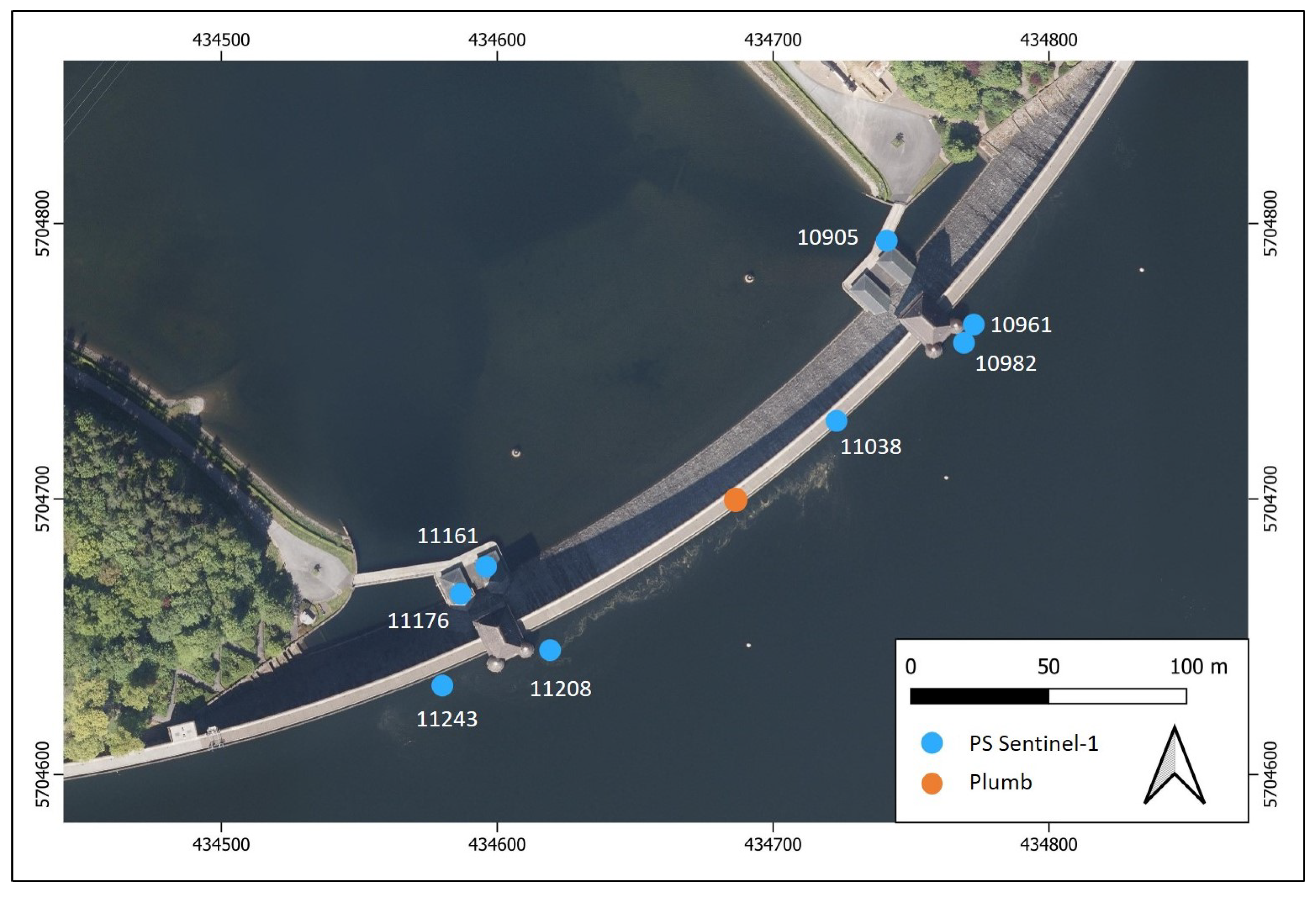
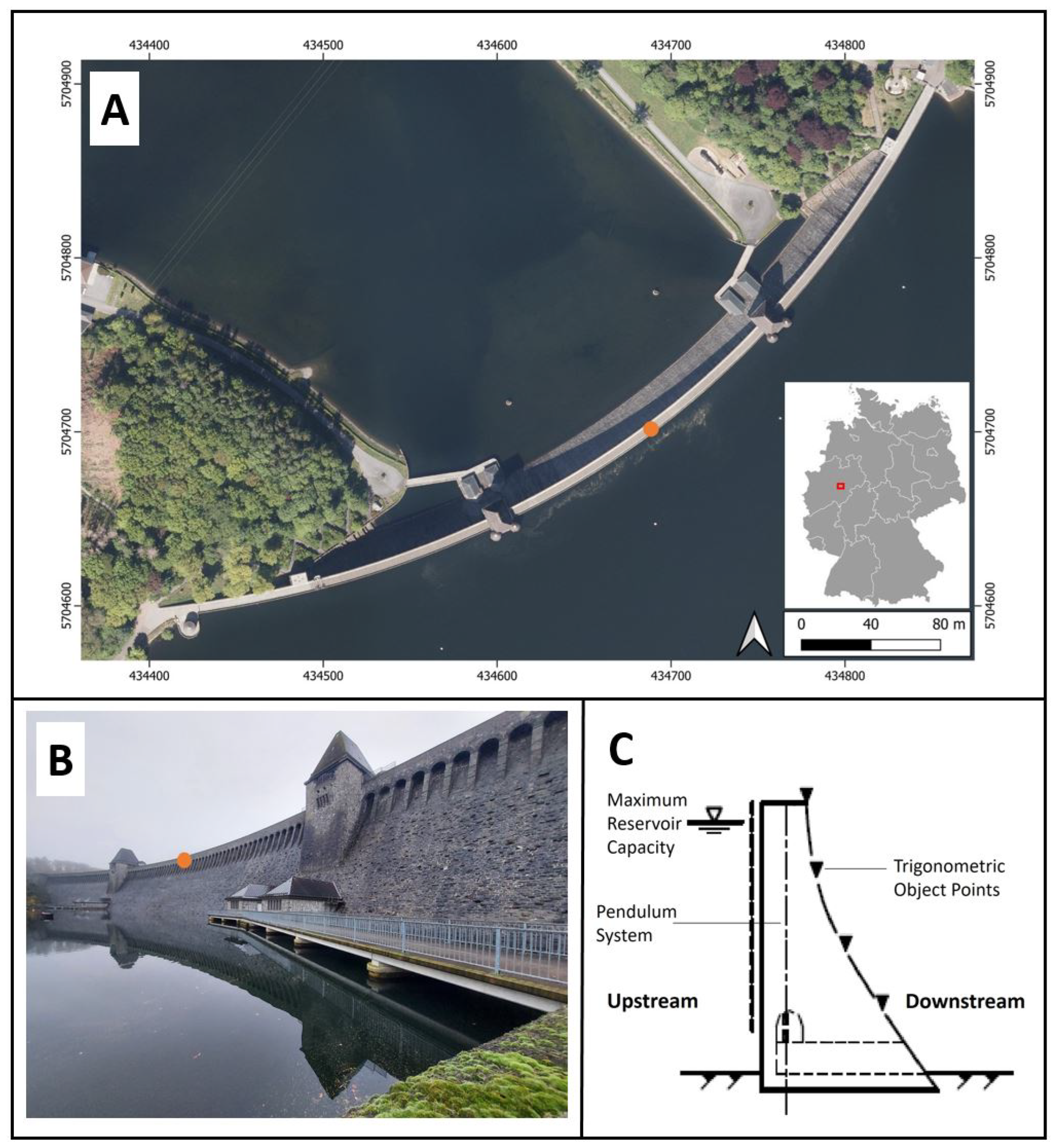
2.1. Study Site

This study was conducted on the Möhne Dam located in the east of North Rhine-Westphalia, western Germany. The dam impounds the Möhne reservoir, which has a total capacity of 134.5 million m³ [23]. The Möhne Dam is a 40 m high arched gravity dam with a crest length of 650 m. The center of its downstream side is oriented towards northwest (320°). Its characteristics are summarized in Figure 1. Built between 1908 and 1912, the Möhne Dam primarily serves as a water supply for the Ruhr area. Additionally, it plays a vital role in energy generation and provides crucial contributions to flood protection and low-water elevation [23]. The dam is operated by the Ruhrverband, a non-profit-oriented water management company. It is equipped with several measuring instruments, such as water level and temperature monitors, trigonometric measurements, and a pendulum system. The pendulum system is located in the center of the dam (see Figure 1A,B).

2.2. Data

2.2.1. In Situ Data

In this study, Sentinel-1 PS time series were utilized for the analysis in addition to in situ data. The timeline of this study spanned from April 2015 to December 2020, with the last 12 months of the time series used as validation data for the prediction. A list of all available in situ data is shown in

Table 2. In situ data used for the analysis, with their corresponding measuring intervals [25].

Data	Temporal Resolution
Pendulum Data (mm)	daily
Water Level (m)	daily
Temperature (°C)	daily

. All variables were provided by the Ruhrverband as daily means.

2.2.2. BBD Data

In situ data were complemented by Sentinel-1 PS time series provided by the BBD, which is operated by the Federal Institute for Geosciences and Natural Resources (BGR). The BBD platform was developed as a WebGIS and provides freely available nationwide deformation information acquired by the Copernicus Sentinel-1 satellites, utilizing the PSI technique [26]. The nationwide PS dataset for Germany is updated on a yearly basis [27]. A dataset spanning from April 2015 to December 2020 was used in the descending line-of-sight direction (LOS) due to its favorable alignment with the dam crest (i.e., S-1 look angle: 276°; radial alignment of the center of the dam crest: 320°) [28]. The time series comprised a total of 287 S-1 interferometric wide-swath (IW) scenes, acquired with a temporal resolution of 12 days. Table 3 summarizes the key characteristics of the dataset. Figure 2 presents the spatio-temporal baseline, with the reference scene indicated by a red dot. The perpendicular baseline for all interferograms in the dataset ranged between −139 m and +167 m, which is well below the critical perpendicular baseline requirement for the C-band [29]. In total, the dataset contained eight PS points associated with the dam, whose locations are shown in Figure 3. Their signal-to-noise ratio (SNR), as provided by BGR, is specified in

Table A1. Signal-to-noise ratio for the PS points of the descending data stack #066 used in this study. SNR values less than 5.0 are not specified by BGR and marked as N/A [30].

Point-ID	SNR
10905	5.8
10961	10.6
10982	5.2
11038	N/A
11161	N/A
11176	16.2
11208	5.9
11243	N/A

.

Table 3. Characteristics of the S-1 IW dataset used in this study [30].

	DESC #066
Start Date	8 April 2015
End Date	31 December 2020
Reference Scene	19 September 2018
No. of Scenes	287
Temporal Resolution	12 days
Incidence Angle	46°
Look Angle	276°
Max. Perpendicular Baseline	+167 m
Min. Perpendicular Baseline	−139 m

Table 3. Characteristics of the S-1 IW dataset used in this study [30].

	DESC #066
Start Date	8 April 2015
End Date	31 December 2020
Reference Scene	19 September 2018
No. of Scenes	287
Temporal Resolution	12 days
Incidence Angle	46°
Look Angle	276°
Max. Perpendicular Baseline	+167 m
Min. Perpendicular Baseline	−139 m

Figure 2. Spatio-temporal baseline plot of the descending S-1 data stack #066 used in this study [31]. A reference scene in the middle of the dataset was selected by BGR for PS processing (i.e., 19 September 2018) [30] and is highlighted with a red dot.

Figure 2. Spatio-temporal baseline plot of the descending S-1 data stack #066 used in this study [31]. A reference scene in the middle of the dataset was selected by BGR for PS processing (i.e., 19 September 2018) [30] and is highlighted with a red dot.

Figure 3. Distribution of PS points of the descending S-1 dataset #066 on the Möhne Dam with their corresponding ID (blue) and the location of the pendulum system in the middle of the dam (orange). Orthophoto: GDI-NRW [24], EPSG: 25832.

Figure 3. Distribution of PS points of the descending S-1 dataset #066 on the Möhne Dam with their corresponding ID (blue) and the location of the pendulum system in the middle of the dam (orange). Orthophoto: GDI-NRW [24], EPSG: 25832.

3. Methods

As previously mentioned, the standard approach to predicting the expected deformation of a dam involves fitting a multiple linear regression with exogenous regressors and trend components. However, the complex deformation behavior of a dam may not be adequately described by such a model. To demonstrate how to enhance this conventional method, a comparison with a more sophisticated model pipeline was conducted. To facilitate this comparison, the standard approach is first described in more detail. Second, the evaluated data-driven approaches are introduced, encompassing advanced model classes and additional feature engineering techniques (e.g., ensemble methods and deep learning approaches). The results of both approaches were analyzed utilizing data acquired from a pendulum system, with a reported accuracy of 0.05 mm [32]. Additionally, PS data from the descending orbit were incorporated into the advanced model pipeline to increase the spatial and temporal resolution of predictions. For monitoring the long-term changes, it is generally advisable to employ a time series spanning several years. To predict the expected deformations of the Möhne Dam for the year 2020 (test data), the period from April 2015 to December 2018 was chosen as the training data to determine the regression coefficients for all models. The year 2019 was selected as the validation period for the trained model. The accuracy of the models was evaluated utilizing descriptive statistics ($R^2$, Mean Absolute Error (MAE)), which are commonly used by dam operators [1,3,25].

3.1. Baseline Model: Multiple Linear Regression Using Pendulum Data

The deformation of a gravity dam is particularly influenced by its exogenous variables and a trend component, (i.e., a linear function of time). For the Möhne Dam, daily means of water level and temperature have been identified by the Ruhrverband as the most dominant factors affecting deformation and were included in the baseline model [25]. In mathematical terms, this is represented by the following Equation (1):

$$Y_t\left[\mathrm{mm}\right]={\beta }_{water}·{water}_t+{\beta }_{temp}·{temp}_t+{\beta }_t·t+{\beta }_0$$

(1)

where Y_t represents the deformation in millimeters, ${\mathit{water}}_t$, ${\mathit{temp}}_t$, and t denote the daily means of water level (m), temperature (°C), and time (days), respectively, with their corresponding slope coefficients ${\beta }_{water}$, ${\beta }_{temp}$, and ${\beta }_t$. ${\beta }_0$ indicates the intercept of the regression model.

3.2. Data-Driven Approach

To improve the deformation prediction, an extensive model search was conducted, which included other model classes, preprocessing of variables, and additional regressors in addition to the results obtained through the baseline model.

Importantly, as a model selection criterion, the time series was split into three subsets. For model selection, we first optimized model parameters on the first split (training; 44 months). We then used this model to predict the second split (validation; 12 months, i.e., the year 2019) to evaluate how well a specific model could extrapolate to new data. This approach also prevented the selection of models that overfit the training data, as such models were unlikely to extrapolate correctly. Finally, we selected the model specification with the highest validation accuracy (MAE) as the final candidate. This model was then retrained on both the training and validation splits and used to predict the entirety of the third split (test), which covered the complete year of 2020. By doing so, we avoided overfitting, as the final performance was reported on a test split that was neither involved in model estimation nor selection.

3.2.1. Model Classes

To achieve an extensive comparison, we leveraged five additional model classes alongside linear regression, which included well-established linear time series prediction techniques, two ensemble methods from the machine learning literature, and novel deep learning approaches.

Concerning time series prediction techniques, we evaluated the following general form of VARMAX (Equation (2)):

$$Y_t\left[\mathrm{mm}\right]=\sum _{i=1}^p{\Phi }_i{Y}_{t-i}+\sum _{j=1}^q{\Theta }_j{ϵ}_{t-j}+A{X}_t+{\mu }_t+{ϵ}_t$$

(2)

Here, $ϵ$ specifies error terms, X holds all exogenous variables considered, and ${\mu }_t$ specifies a trend. $\Phi$, $\Theta$, and A are parameters that are estimated (referenced as “ari” in ARIMAX). $Y_{t-i}$ marks the past deformation value in millimeters i days ago. Importantly, while this is often not relevant for pendulum measurements, previous studies have shown that interactions between PS points are possible, depending on where they are located on the dam [21]. Therefore, we also evaluated a vectorized form of this model, in which each vector held all PS points in one direction (referenced as “var” in VARMAX). In both cases, implementations provided by statsmodels [33] were utilized. Notably, in the special case where p and q are zero, the model class converges to a simple linear regression in its non-vectorized form, as the only regressors that remain are the influences specified in Equation (2).

Regarding the ensemble methods, we deployed random forests (rf) [34] and AdaBoost (ada) [35]. Both strategies rely on fitting multiple weak learners (e.g., simple regression trees) and combining them into a more robust model. Notably, due to their compositional nature, both methods can represent nonlinear relationships between regressors and the target variable. In both cases, the implementation provided by Pedregosa et al. [36] was used.

Finally, to cover recent trends in the machine learning literature, we deployed two deep learning approaches, tfm and Chronos [37]. Since the time series data were limited, fitting neural networks from scratch was deemed infeasible for now. Further information on the functionality of foundational time series models can be found in Liang et al. [38].

As a general idea, we aimed to evaluate model classes with various levels of complexity and capabilities, as we did not want to make assumptions about what works for the presented data distribution. While VARMAX models are inherently unable to model nonlinear interactions between regressors and target time series, they are robust against overfitting. On the other hand, ensemble methods might catch potential nonlinear interactions and thus improve predictions, while being more likely to overfit. By also including foundational models, which somehow exist outside of the classic bias–variance tradeoff, we attempted to sample from the full spectrum of potential forecasting techniques.

3.2.2. Exogenous Variables

While it is expected that the air temperature and the water level of the current day explain a considerable amount of the variance in dam deformation, additional regressors may further improve prediction accuracy. To test this, the following potential candidates were evaluated: First, past values of air temperature and water level, either as daily means or weekly means, were considered. Given that the movement of dams under normal conditions is generally slow, these additional regressors have the potential to further improve prediction accuracy by representing the historical environmental context. Consequently, they provide a beneficial constraint on predicting the next step, especially if the values of an exogenous variable differ considerably between consecutive time steps. Thus, we considered past values as additional regressors.

Second, interaction effects were evaluated to account for potential multiplicative effects of air temperature and water level on dam movement. The following two interaction effects were tested (Equations (3) and (4)):

$${water}_t·{temp}_t$$

(3)

$${\displaystyle \frac{{water}_t-{water}_{min}}{{water}_{max}-{water}_{min}}}·{\displaystyle \frac{{temp}_t-{temp}_{min}}{{temp}_{max}-{temp}_{min}}}$$

(4)

Here, ${water}_{min}$, ${temp}_{min}$, and ${water}_{max}$, ${temp}_{max}$ represent the minimum and maximum values for water level and temperature over the entire time series. In particular, Equation (3) represents the simplest form of interaction effect that can be defined. However, temperature, and consequently the interaction effect, can assume negative values. To address this, Equation (4) was also considered, where both water level and temperature are scaled between 0 and 1, thereby eliminating this potentially disruptive yet informative sign change.

Third, we evaluated a strategy in which the regressors, as well as the target time series, were detrended and deseasoned (annual cycle). The intuition behind this approach is to abstract long-term patterns from the time series, allowing models to focus solely on deviations from these long-term trends, which could be an indicator of anomalous deformations. This step involved first fitting a linear regression with time for each variable and removing the regressions’s prediction from the time series. Subsequently, a sinusoid with a frequency of one year was fitted to the data and subtracted.

Finally, a set of preprocessing steps was performed independently of model specifications. First, a data split into training and testing sets was conducted to prevent information flow from the training data into the testing data. Parameters for min–max normalization were calculated based on the training data and then applied to both the training and testing sets. For the training data, outlier filtering was performed by detrending and applying boxplot filtering. Additionally, missing values in the training data were linearly interpolated.

3.2.3. Model Search

To identify the best model for describing a specific time series of dam deformation, we evaluated a comprehensive set of potential model classes in conjunction with all possible combinations of additional regressors, including models that omit certain features down to the baseline model. Additionally, AdaBoost and random forests both have multiple hyperparameters, which we evaluated as follows: maximum depth of the decision trees (random forest), learning rate (ada), baseline estimator (ada), and the number of base models (ada and random forest). In total, we evaluated over 20,000 models for each time series and selected those yielding the highest validation performance, as described in Section 3.2. The detailed model search space is specified in

Table 4. Evaluated model search space to identify the most suitable model. A “-” indicates that the corresponding variable was not utilized. “DT” represents a decision tree model, while “Lin” denotes a simple linear regression model. All possible variable combinations were assessed. No hyperparameter tuning was performed for the foundational models, as the target time series was analyzed in its raw form.

	Linear	Arimax	VARMAX	Random Forest	AdaBoost
$T{S}_{t-n}$ (P, Equation (2))	-, 1, 2	-, 1, 2	-, 1, 2	-, 1, 2	-, 1, 2
$W_{t-n}$	-, 0, 1, 2	-, 0, 1, 2	-, 0, 1, 2	-, 0, 1, 2	-, 0, 1, 2
$T_{t-n}$	-, 0, 1, 2	-, 0, 1, 2	-, 0, 1, 2	-, 0, 1, 2	-, 0, 1, 2
$W^M$	-, 7	-, 7	-, 7	-, 7	-, 7
$T^M$	-, 7	-, 7	-, 7	-, 7	-, 7
Decomposition	Y, N	Y, N	Y, N	Y, N	Y, N
Interaction Effect	-, (3), (4)	-, (3), (4)	-, (3), (4)	-, (3), (4)	-, (3), (4)
Estimator	-	-	-	-	DT, Lin
N Estimators	-	-	-	50, 250	50, 250
Learning Rate	-	-	-	-	1, 0.1
Max Depth	-	-	-	-, 3, 7	-
D (Equation (2))	-	0, 1	-	-	-
Q (Equation (2))	-	0, 1, 2	0, 1, 2	-	-

. While the full model search incurred some computational overhead that could be parallelized, individual model estimations and inference entailed only minimal computational costs—typically within single-digit seconds on an Intel^® Core™ i7 CPU.

4. Results

This section presents the results of this study and is divided into two parts: First, the model output of the data-driven algorithms is presented for the pendulum data, along with an evaluation of the obtained accuracies compared to the linear regression model. Second, the model outputs of the data-driven approaches for the PS data are presented, along with the identification of the drivers of deformation.

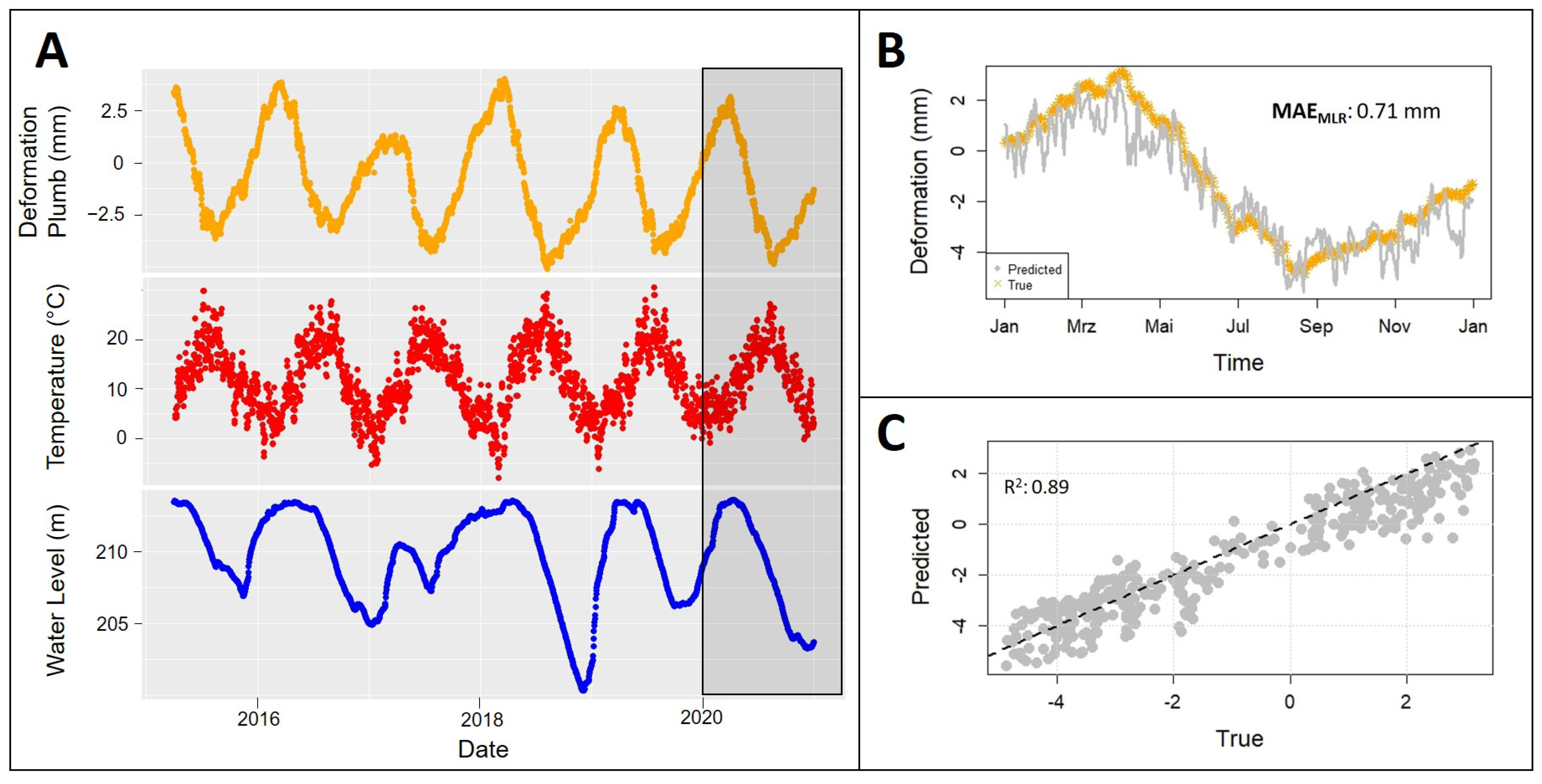
4.1. Deformation Prediction Obtained Through In Situ Data and Pendulum Measurements

As shown in Figure 4, the baseline model indicated a strong relationship between the predicted deformation values and the pendulum data ($R^2$ = 0.89). The MAE was 0.71 mm, with extreme values ranging from −3.30 mm (underprediction) to +1.58 mm (overprediction). For the Möhne Dam, the fit of the linear model resulted in the following regression coefficients, as shown in Equation (5):

$$Y_t\left[\mathrm{mm}\right]=0.45·{water}_t-0.24·{temp}_t-0.0005·t-9.28$$

(5)

As evident from this model parametrization, daily changes in water level and temperature had the strongest influence on dam deformation, manifesting as a downstream deformation of 0.45 mm for every 1 m rise in water level. Conversely, temperature counteracted the effect of water level by inducing an upstream deformation of −0.24 mm for every 1 °C increase in temperature. This relationship is well known and extensively described in the literature [1,3,5]. Although the trend component appeared considerably smaller at −0.0005 mm per day, it resulted in an annual deformation towards the upstream side of −0.18 mm.

To disentangle the effects of various potential upgrades on the baseline model’s prediction accuracy, multiple subsets of additional regressors were evaluated. Alongside the baseline, which only used the current air temperature and water level along with some trend components, models that utilized all possible additional regressors except the autoregressive information (i.e., information connected to historic values) of the target time series are displayed in Figure 5. Subsequently, models treating the target time series as univariate (i.e., with no exogenous regressors) are presented. Finally, the model resulting from the full model search space is reported, where all possible regressors are evaluated.

As observed in Figure 5, the prediction performance of the baseline model could be enhanced by utilizing data-driven algorithms, reducing the mean absolute prediction error from 0.51 mm to as low as 0.05 mm with the full model search space. However, considerable differences exist among the various algorithms and search spaces. The accuracy of the baseline model ($MA{E}_{best}$: 0.51 mm) could be improved by incorporating additional exogenous variables ($MA{E}_{best}$: 0.38 mm), as well as utilizing the full search space ($MA{E}_{best}$: 0.05 mm). $R^2$ was maximized from 0.92 in the baseline model to 0.99 when utilizing the full model search space.

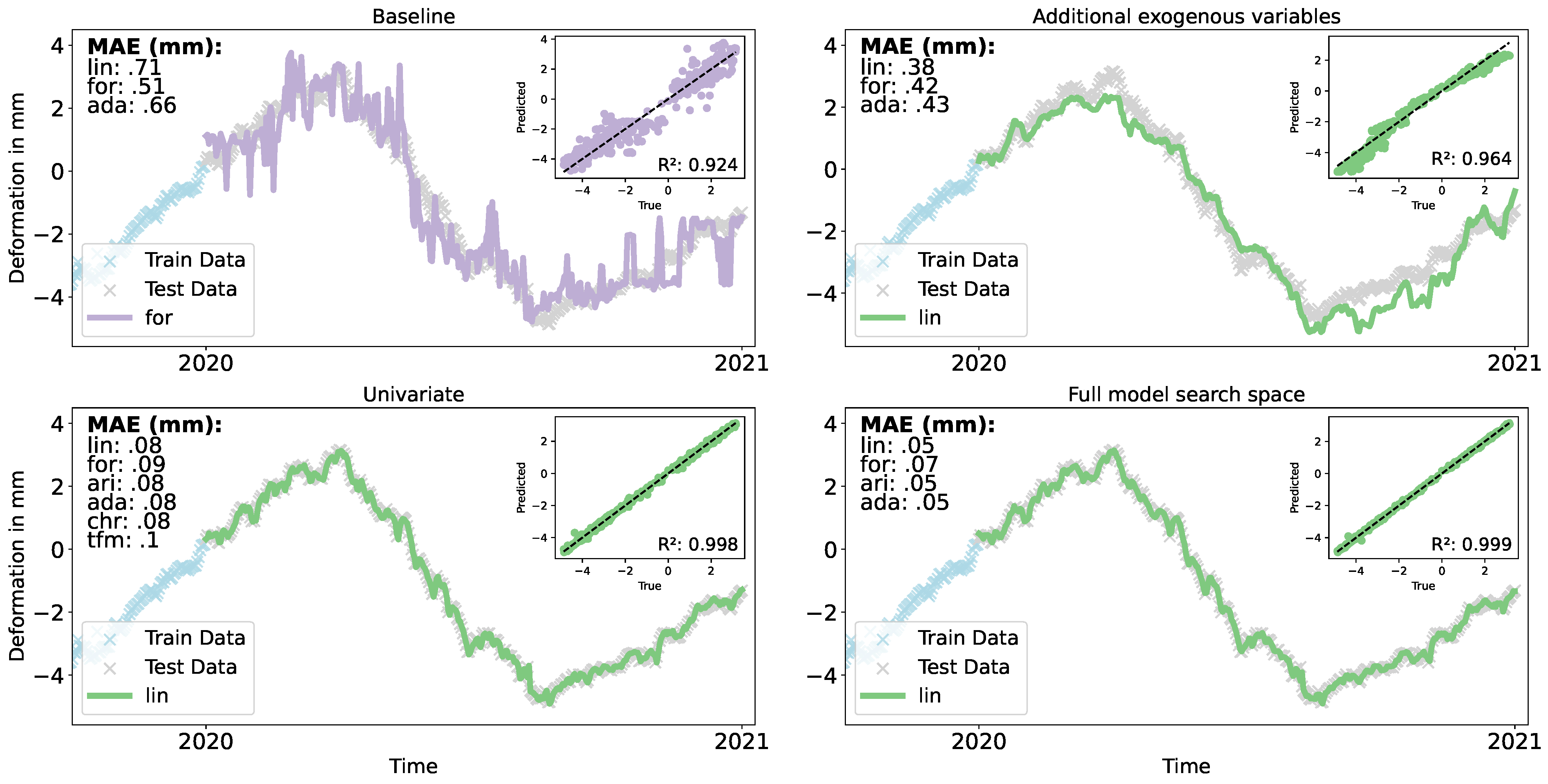
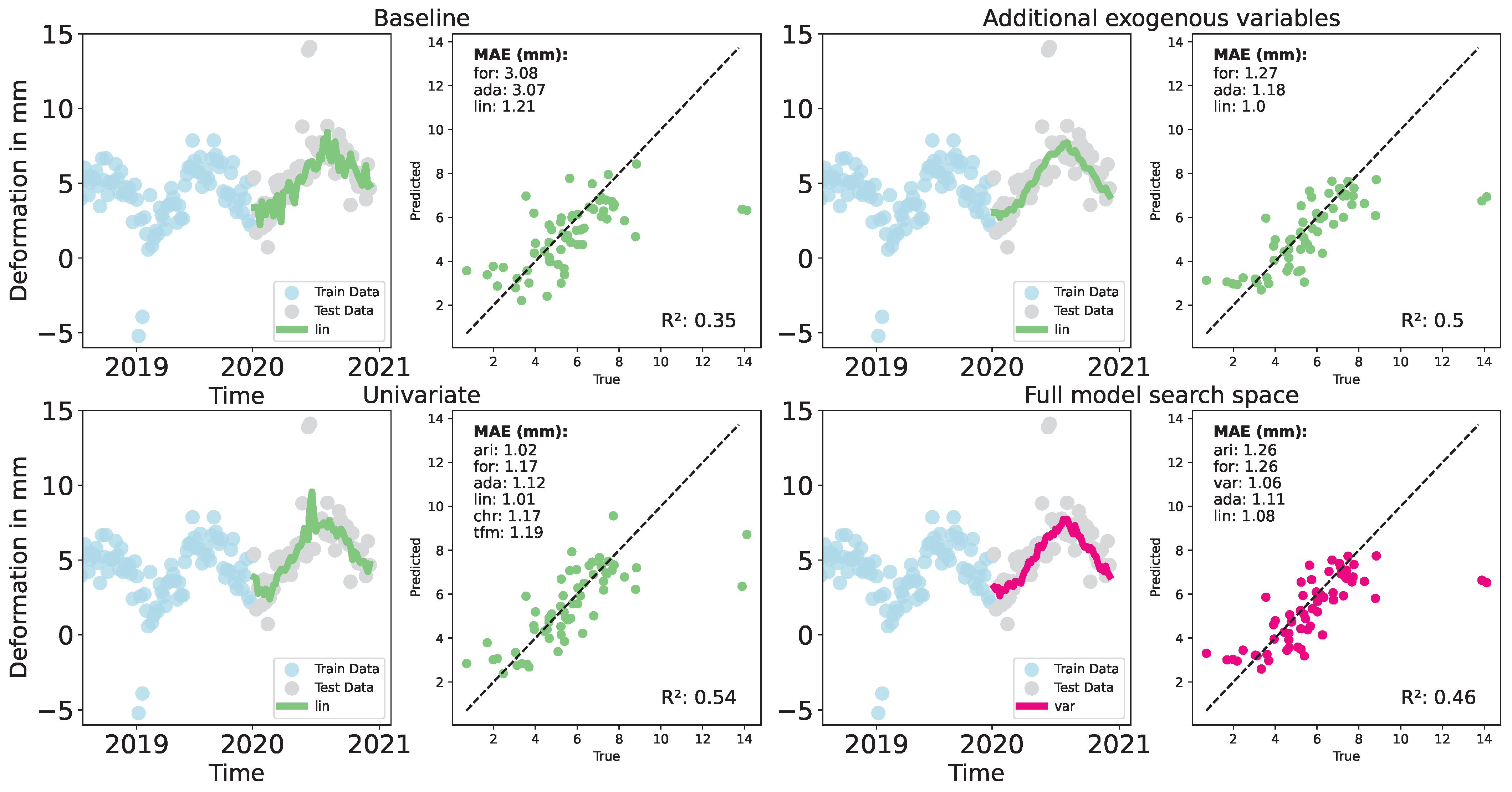
4.2. Deformation Prediction Obtained Through In Situ Data and Sentinel-1 PS Time Series

Considering the Sentinel-1 PS time series, the exact model specifications, particularly the model classes, differed for each PS point. While this is less straightforward, differences in deformation patterns were expected since the PS points lie on different sections of the dam (see Figure 3). Gains in prediction accuracy were generally smaller compared to pendulum data, because the signal-to-noise ratio was much lower. As evident in

Table 5. Prediction accuracy (MAE in mm) per search space for all PS points of the descending LOS direction. Model classes are denoted in the following way: linear (lin), ARIMAX (ari), AdaBoost (ada), time series foundational model (tfm), Chronos (chr), random forest (for), and VARMAX (var).

Search Space	Model Class	10905	10961	10982	11038	11161	11176	11208	11243
Baseline	lin	1.52	1.02	1.18	3.85	2.05	1.21	1.56	3.16
	for	3.41	3.03	3.71	5.01	3.03	3.08	2.76	4.18
	ada	3.48	3.06	3.62	4.84	2.83	3.07	2.53	3.93
Baseline + Exogenous	lin	1.56	0.98	1.12	3.64	2.09	1.00	1.42	3.26
	for	1.72	1.39	1.24	4.18	2.23	1.27	1.49	3.27
	ada	1.57	1.81	1.34	4.66	2.19	1.18	1.57	3.51
Univariate	lin	1.50	0.81	1.06	3.72	2.06	1.01	1.40	3.25
	ari	1.34	0.94	1.06	3.73	2.05	1.02	1.39	3.26
	for	1.64	1.02	1.50	4.09	2.22	1.17	1.76	3.27
	ada	1.40	0.84	0.97	3.68	2.10	1.12	1.65	3.11
	tfm	1.50	0.88	1.16	4.18	2.16	1.19	1.54	3.34
	chr	1.55	0.87	1.17	4.22	2.28	1.17	1.69	3.40
Full	lin	1.51	0.98	1.08	3.59	2.04	1.08	1.42	3.26
	ari	1.86	1.05	1.44	3.71	2.74	1.26	1.61	4.26
	var	1.56	1.09	1.13	3.64	2.11	1.06	1.42	3.37
	for	1.72	0.95	1.24	4.21	2.04	1.26	1.49	3.27
	ada	1.57	0.93	1.34	4.55	2.19	1.11	1.57	3.21
	tfm	1.50	0.88	1.16	4.18	2.16	1.19	1.54	3.34
	chr	1.55	0.87	1.17	4.22	2.28	1.17	1.69	3.40

, the accuracy of all predictions could be improved compared to the baseline model. Interestingly, the full search space yielded the lowest prediction errors for only two of the eight PS points (ID #11038, #11161). It is suspected that the comparatively low resolution and low signal-to-noise ratio of the time series might favor such phenomena as more model search increases the probability of a model overfitting on training data. These phenomena should be noted when deploying such search strategies in the future.

Table 6. Feature usage of the selected and displayed models for each PS point of the descending line of sight. Notably, no clear trends could be determined. W denotes water level, and T denotes temperature. Time lags are specified with t-n. Mean values of specified periods (here seven days) are specified with M. Multiplicative effects are denoted as Interaction. Furthermore, $Decompose$ specifies if the data were detrended and deseasoned before predictions. Notably, MAE is calculated for the original data values by adding trend and season to the predictions.

	10905	10961	10982	11038	11161	11176	11208	11243
$W_t$	✗	✗	✓	✓	✗	✗	✓	✓
$T_t$	✗	✗	✗	✓	✓	✓	✓	✓
$W_{t-n}$	✗	✗	✗	✗	✗	✗	✓	✓
$T_{t-n}$	✗	✗	✗	✓	✓	✗	✓	✓
$W_7^M$	✗	✗	✓	✗	✗	✗	✗	✗
$T_7^M$	✗	✗	✓	✓	✗	✓	✗	✓
Interaction	✗	✗	✓	✓	✓	✗	✓	✗
Decompose	✗	✗	✓	✓	✓	✓	✓	✓

summarizes the feature usage of the selected models for each PS point of the descending line of sight, identifying the models’ main drivers. Importantly, the final specifications varied for each PS point, with the air temperature of the current day ($T_t$) identified as the most frequently used parameter. Furthermore, interaction effects played a major role, suggesting that the effects of water level and temperature on dam deformation are indeed multiplicative. Regarding decomposition, all PS points—except for the two best predicted by a foundational model (i.e., #10905, #10961)—utilized decomposition, highlighting its usefulness for non-foundational approaches. For foundational models, only the raw time series was provided without further processing. Finally, additional influences differed from model to model. Given that the PS points lie in different dam sections (see Figure 3), this variation was considered a valid phenomenon. Therefore, selecting the regressors for each model individually proved highly beneficial.

Figure 6 compares the baseline model and the best-performing model from the full search space for all PS points. Since the model search space deployed depends on the specific needs of experts and dam operators, we refrain from making more interpretations concerning appropriate model search spaces here. However, we state that the baseline approach could be improved in all cases, positioning the approach as useful, regardless of the specified model search space. Furthermore, the fact that almost no improvement was possible for PS points #11243 and #11161 (as shown in Table 5) might indicate that not all points are suitable for inclusion in a valid monitoring strategy. For these two points, this could most likely be attributed to a very poor signal-to-noise ratio. They can be filtered a priori.

In summary, this extended model pipeline improved prediction accuracy in both pendulum measurements and PS time series, making it highly recommended, regardless of the monitoring strategy.

5. Discussion

The proposed approach enabled a considerable improvement in deformation predictions for a gravity dam through data-driven approaches, utilizing both pendulum and PS data. While we evaluated a wide range of time series prediction techniques, it is possible that additional model classes could provide further improvements over the current accuracy. However, this study provided evidence that the introduction of large model searches is promising, especially when autoregressive components and exogenous variables are available for prediction.

The findings of this study indicated that the deformation behavior of the Möhne Dam follows a seasonal cycle, characterized by movements towards both the upstream and downstream sides, as previously reported in the literature [1,3,19]. Similar improvements in deformation prediction accuracy are likely achievable for other gravity dams, as demonstrated by Stein et al. [21]. Furthermore, while our methodology is expected to be applicable to different dam types, such as embankment dams, predicting specific effects, such as the permanent settlement of the dam body due to the consolidation of fill material [4], may be more challenging. Consequently, the prediction accuracy for these types of dams may be lower compared to gravity dams. Nevertheless, it is important to emphasize that the proposed methodology was designed to identify the baseline model as the optimal choice when no further enhancements are feasible, making its application advantageous regardless of the dam type.

A notable observation was made where reducing the model search space resulted in the identification of better models for six out of the eight PS points (see Table 5). Figure 7 illustrates this phenomenon for PS point #11176, demonstrating the variations in prediction accuracy as a function of the model search space. Although several factors, including signal-to-noise ratio, overfitting, and the interaction between sample size and search space, may have contributed to this outcome, a detailed interpretation lies beyond the scope of this study. It is important to emphasize, however, that the selection of PS points and model classes for dam monitoring ultimately lies with the operators. Furthermore, PS points that are more robustly predicted using univariate models (i.e., models that exclude exogenous influences) should be approached with caution, as it is well established that exogenous factors account for the majority of typical movements on a gravity dam. In such cases, filtering these points should be considered as a preprocessing step prior to analysis.

While we evaluated the potential of newly released foundational models, their current univariate structure limits their capacity to account for the interactions among multiple variables, thereby constraining their utility. Given that multivariate foundational models will become a reality in the future, they should be integrated into the model search space.

For PS-based deformation prediction, we utilized analysis-ready Sentinel-1 datasets provided by the German Ground Motion Service (BBD). While BBD data are updated only annually, which may not fulfill the critical requirements for operational dam monitoring, our approach remained independent of the data source used for analysis. As an alternative, data provided by the European Ground Motion Service (EGMS), now including LOS measurements in its recent update, can be considered. In contrast to BBD data, EGMS performs multi-temporal interferometric processing using both persistent scatterers and distributed scatterers (DSs) [39,40]. While the PS technique relies on single dominant scatterers with a high-quality interferometric phase [41], the DS approach focuses on areas of moderate coherence, where multiple neighboring pixels exhibit similar reflectivity values, as they belong to the same object [42]. Unlike PS, distributed scatterers lack a single dominant reflector, making the technique particularly useful in rural areas with lower coherence. On the one hand, combining both techniques, as implemented in EGMS, increases the number of measurement points available for deformation monitoring. On the other hand, filtering points with low temporal coherence or a poor signal-to-noise ratio is crucial. Otherwise, several dozen PS points on a dam may be far less effective for decision-making than a smaller number of high-quality points. The BBD datasets used in this study were provided by the BGR as analysis-ready, pre-filtered PS time series based on their temporal coherence to ensure quality standards. However, if the data quality by either BBD or EGMS does not meet the requirements of dam operators, independent processing of PS time series remains an option. This approach entails considerable time and cost investments.

Filtering PS points is crucial, as decision-making is based on the reliable detection of ongoing deformations on the dam. Various methods have been implemented for phase denoising, including traditional local filters, transformed-domain filters, and nonlocal filters [43]. Additionally, outliers in the PS time series can be filtered, as they may disturb model estimation. In our experiments, we applied boxplot filtering to the time series, removing values that fall outside the 2.25 interquartile range of the dataset’s distribution. As a result, in the case of PS point #11176, all outliers with deviations exceeding 5 mm were removed. We retained these filtered values in the visualizations of the time series to illustrate their frequency of occurrence (see Figure 7). Importantly, more advanced filtering techniques that account for seasonal anomalies could be implemented in future research. Ultimately, the preselection of PS points should be considered for effective decision-making. In this study, three of the eight PS points exhibited an SNR below 5.0 (ID #11038, #11161, #11243), making the interpretation of ongoing deformations on the dam more challenging.

Finally, it should be noted that the PS data and pendulum measurements were treated separately in this work. These monitoring strategies measure different movement directions (i.e., LOS and radial deformations) and exhibited vastly different signal-to-noise ratios. By utilizing data-driven approaches, the accuracy of predictions obtained through pendulum data could be considerably enhanced. For PS data predictions, these novel approaches also proved valuable, even if performance gain in comparison to established approaches depends on the specific PS point (see Table 5). It is important to note that the aim of this study was not to achieve the same model accuracies with PS data as with pendulum data. Unsurprisingly, the model accuracy for pendulum measurements was about an order of magnitude higher ($MA{E}_{max}$: 0.05 mm) than that for PS data ($MA{E}_{max}$: 0.81 mm). Normalization allows comparing LOS deformations with those of the pendulum system [4]. This requires the absence of significant vertical deformations and an optimal alignment of the dam with the sensor’s look direction [28]. In this study, we used a dataset in the descending direction; however, the approach can also be applied to datasets from the ascending direction. It is important to emphasize that our methodology provided increased model accuracy regardless of the data used for prediction.

Although PS-based techniques are still novel and not yet integrated into operational services, they can be highly beneficial for dam monitoring. This is not only due to their higher spatial density, which allows for more comprehensive monitoring of all dam sections, but also because of their feasible temporal resolution, which enables monitoring every 12 days. Recent studies have shown that utilizing PS data for deformation monitoring can be highly beneficial for dam operators [6,15]. This is particularly the case on dams where no pendulum data are available. Therefore, we recommend incorporating the proposed methodology into the monitoring program of gravity dams, utilizing freely available PS datasets as a complement to in situ measurements.

6. Conclusions

This study investigated the potential of utilizing advanced data-driven techniques and additional feature engineering to improve the prediction of dam deformations, as represented through pendulum measurements or PS datasets. By conducting an extensive model search, we provide evidence for the following insights: First, we found that additional feature engineering can considerably enhance model accuracy, although the improvement is substantially greater for pendulum data, reducing the mean absolute error from 0.51 mm in the baseline model ($R^2$ = 0.92) to as low as 0.05 mm using the full model search space ($R^2$ = 0.99). Second, integrating freely available PS datasets with spatially and temporally confined in situ measurements could considerably enhance dam monitoring, establishing MT-InSAR as a valuable tool for dam operators—particularly on dams where no pendulum systems are installed. Although the model accuracy for PS datasets ($MA{E}_{max}$: 0.81 mm) was approximately one order of magnitude lower than that for pendulum data, the mean absolute prediction error could be reduced by up to 0.25 mm using the proposed approach. For implementation into operational monitoring programs, adequate dataset filtering is essential to eliminate noisy PS points. Third, incorporating extended representations of water level and temperature, including the interaction effects between both of them, could further improve model accuracy and reduce prediction errors. With these insights, we recommend incorporating the proposed approach into the monitoring program of gravity dams to accurately predict expected deformations.

Regarding future work, incorporating additional exogenous variables, such as frost and groundwater levels, is expected to further increase accuracy. Additionally, expanding the analysis of gravity dam deformations to consider actual physical mechanisms, rather than merely correlational patterns, may be of great interest. This also applies to other dam types, such as embankment dams.

References

1. Böcker, D.; Schumann, A.; Bettzieche, V. Analysis of Shifts and Trends of Monitoring Data at Dams with Consideration of the Influence of Variables Measured Externally. JOT-Int. Surf. Technol. 2010, 3, 8–11. [Google Scholar] [CrossRef]
2. German Association for Water and Waste (DWA). Mess- und Kontrolleinrichtungen zur Überprüfung der Standsicherheit von Staumauern und Staudämmen. In DVWK-Merkblätter zur Wasserwirtschaft; Parey-Verlag Hamburg: Hamburg, Germany, 1991; Volume Heft 222. [Google Scholar]
3. Bettzieche, V. Mathematical-Statistical Analysis of Measurements from Dam Monitoring. Wasserwirtschaft 2004, 94, 30–34. [Google Scholar] [CrossRef]
4. Bettzieche, V. Satellite monitoring of the deformations of dams. Wasserwirtschaft 2020, 110, 48–51. [Google Scholar] [CrossRef]
5. Fleischer, H. Load-bearing behaviour of old dams and conclusions for structural monitoring. Wasserwirtschaft 2022, 112, 12–18. [Google Scholar] [CrossRef]
6. Milillo, P.; Perissin, D.; Salzer, J.T.; Lundgren, P.; Lacava, G.; Milillo, G.; Serio, C. Monitoring dam structural health from space: Insights from novel InSAR techniques and multi-parametric modeling applied to the Pertusillo dam Basilicata, Italy. Int. J. Appl. Earth Obs. Geoinf. 2016, 52, 221–229. [Google Scholar] [CrossRef]
7. Corsetti, M.; Fossati, F.; Manunta, M.; Marsella, M. Advanced SBAS-DInSAR technique for controlling large civil infrastructures: An application to the Genzano di Lucania dam. Sensors 2018, 18, 2371. [Google Scholar] [CrossRef]
8. Bayik, C.; Abdikan, S.; Arıkan, M. Long term displacement observation of the Atatürk Dam, Turkey by multi-temporal InSAR analysis. Acta Astronaut. 2021, 189, 483–491. [Google Scholar] [CrossRef]
9. Grebby, S.; Sowter, A.; Gluyas, J.; Toll, D.; Gee, D.; Athab, A.; Girindran, R. Advanced analysis of satellite data reveals ground deformation precursors to the Brumadinho Tailings Dam collapse. Commun. Earth Environ. 2021, 2, 2. [Google Scholar] [CrossRef]
10. Milillo, P.; Porcu, M.C.; Lundgren, P.; Soccodato, F.; Salzer, J.; Fielding, E.; Bürgmann, R.; Milillo, G.; Perissin, D.; Biondi, F. The ongoing destabilization of the Mosul dam as observed by synthetic aperture radar interferometry. In Proceedings of the 2017 IEEE International Geoscience and Remote Sensing Symposium (IGARSS), Fort Worth, TX, USA, 23–28 July 2017; pp. 6279–6282. [Google Scholar] [CrossRef]
11. Ruiz-Armenteros, A.M.; Lazecky, M.; Hlaváčová, I.; Bakoň, M.; Delgado, J.M.; Sousa, J.J.; Lamas-Fernández, F.; Marchamalo, M.; Caro-Cuenca, M.; Papco, J.; et al. Deformation monitoring of dam infrastructures via spaceborne MT-InSAR. The case of La Viñuela (Málaga, southern Spain). Procedia Comput. Sci. 2018, 138, 346–353. [Google Scholar] [CrossRef]
12. Othman, A.A.; Al-Maamar, A.F.; Al-Manmi, D.A.M.; Liesenberg, V.; Hasan, S.E.; Al-Saady, Y.I.; Shihab, A.T.; Khwedim, K. Application of DInSAR-PSI technology for deformation monitoring of the Mosul Dam, Iraq. Remote Sens. 2019, 11, 2632. [Google Scholar] [CrossRef]
13. Abo, H.; Osawa, T.; Ge, P.; Takahashi, A.; Yamagishi, K. Deformation Monitoring of Large-Scale Rockfill Dam Applying Persistent Scatterer Interferometry (PSI) Using Sentinel-1 SAR Data. In Proceedings of the IEEE 2021 7th Asia-Pacific Conference on Synthetic Aperture Radar (APSAR), Virtual, 1–3 November 2021; pp. 1–6. [Google Scholar] [CrossRef]
14. Marchamalo-Sacristán, M.; Ruiz-Armenteros, A.M.; Lamas-Fernández, F.; González-Rodrigo, B.; Martínez-Marín, R.; Delgado-Blasco, J.M.; Bakon, M.; Lazecky, M.; Perissin, D.; Papco, J.; et al. MT-InSAR and dam modeling for the comprehensive monitoring of an Earth-fill dam: The case of the Benínar dam (Almería, Spain). Remote Sens. 2023, 15, 2802. [Google Scholar] [CrossRef]
15. Marchamalo-Sacristán, M.; Fernández-Landa, A.; Sancho, C.; Hernández-Cabezudo, A.; Krishnakumar, V.; García-Lanchares, C.; Sánchez, J.; Rubén, M.M.; Rejas-Ayuga, J.; González-Tejada, I.; et al. EyeRADAR-Dam: Integration of MT-InSAR with monitoring technologies in a pilot monitoring system for embankment dams. Procedia Comput. Sci. 2024, 239, 2286–2292. [Google Scholar] [CrossRef]
16. Wang, Z.; Perissin, D. Cosmo SkyMed AO projects-3D reconstruction and stability monitoring of the Three Gorges Dam. In Proceedings of the 2012 IEEE International Geoscience and Remote Sensing Symposium, Munich, Germany, 22–27 July 2012; pp. 3831–3834. [Google Scholar] [CrossRef]
17. Lazecky, M.; Perissin, D.; Lei, L.; Qin, Y.; Scaioni, M. Plover Cove dam monitoring with spaceborne InSAR technique in Hong Kong. In Proceedings of the 2nd Joint International Symposium on Deformation Monitoring, Nottingham, UK, 9–11 September 2013; pp. 9–11. Available online: http://www.sarproz.com/wp-content/papercite-data/pdf/lazecky-pcdmwsitihk2013.pdf (accessed on 11 October 2024).
18. Tomás, R.; Cano, M.; Garcia-Barba, J.; Vicente, F.; Herrera, G.; Lopez-Sanchez, J.M.; Mallorquí, J. Monitoring an earthfill dam using differential SAR interferometry: La Pedrera dam, Alicante, Spain. Eng. Geol. 2013, 157, 21–32. [Google Scholar] [CrossRef]
19. Jänichen, J.; Schmullius, C.; Baade, J.; Last, K.; Bettzieche, V.; Dubois, C. Monitoring of Radial Deformations of a Gravity Dam Using Sentinel-1 Persistent Scatterer Interferometry. Remote Sens. 2022, 14, 1112. [Google Scholar] [CrossRef]
20. Dubois, C.; Ziemer, J.; Jänichen, J.; Stumpf, N.; Liedel, C.; Sabrowski, M.; Schmullius, C. Dam Monitoring with Ground Motion Services—A Case Study of a Gravity Dam with the German Ground Motion Service. In Proceedings of the IGARSS 2024-2024 IEEE International Geoscience and Remote Sensing Symposium, Athens, Greece, 7–12 July 2024; pp. 4670–4673. [Google Scholar] [CrossRef]
21. Stein, G.; Ziemer, J.; Wicker, C.; Jänichen, J.; Demisch, G.; Klöpper, D.; Last, K.; Denzler, J.; Schmullius, C.; Shadaydeh, M.; et al. Data-Driven Prediction of Large Infrastructure Movements Through Persistent Scatterer Time Series Modeling. In Proceedings of the IGARSS 2024-2024 IEEE International Geoscience and Remote Sensing Symposium, Athens, Greece, 7–12 July 2024; pp. 8669–8673. [Google Scholar] [CrossRef]
22. Rana, N.M.; Delaney, K.B.; Evans, S.G.; Deane, E.; Small, A.; Adria, D.A.; McDougall, S.; Ghahramani, N.; Take, W.A. Application of Sentinel-1 InSAR to monitor tailings dams and predict geotechnical instability: Practical considerations based on case study insights. Bull. Eng. Geol. Environ. 2024, 83, 204. [Google Scholar] [CrossRef]
23. Ruhrverband. Möhnetalsperre. Sicherheitsbericht. Teil A. Unpublished Security Report. 2013. [Google Scholar]
24. GDI-NRW. Geodateninfrastruktur Nordrhein-Westfalen. Geoportal NRW. 2021. Available online: https://www.gdi.nrw (accessed on 11 October 2024).
25. Ruhrverband. Möhnetalsperre. Vertiefte Überprüfung. Analyse der Messdaten. Unpublished Security Report. 2018. [Google Scholar]
26. Kalia, A.; Frei, M.; Lege, T. A Copernicus downstream-service for the nationwide monitoring of surface displacements in Germany. Remote Sens. Environ. 2017, 202, 234–249. [Google Scholar] [CrossRef]
27. Kalia, A.C.; Frei, M.; Lege, T. BodenBewegungsdienst Deutschland (BBD): Konzept, Umsetzung und Service-Plattform. ZfV-Z. Geod. Geoinf. Landmanag. 2021, 4. [Google Scholar] [CrossRef]
28. Ziemer, J.; Jänichen, J.; Wicker, C.; Klöpper, D.; Last, K.; Kalia, A.; Lege, T.; Schmullius, C.; Dubois, C. Assessing the Feasibility of Persistent Scatterer Data for Operational Dam Monitoring in Germany: A Case Study (submitted). Remote Sens. 2025. [Google Scholar]
29. Kumar, H.; Syed, T.H.; Amelung, F.; Agrawal, R.; Venkatesh, A. Space-time evolution of land subsidence in the National Capital Region of India using ALOS-1 and Sentinel-1 SAR data: Evidence for groundwater overexploitation. J. Hydrol. 2022, 605, 127329. [Google Scholar] [CrossRef]
30. BGR. Federal Institute for Geosciences and Natural Resources. BodenBewegungsdienst Deutschland (BBD). 2020. Available online: https://bodenbewegungsdienst.bgr.de/mapapps/resources/apps/bbd/index.html?lang=de (accessed on 11 October 2024).
31. Alaska Satellite Facility. ASF DAAC Vertex Data Search. 2025. Available online: https://search.asf.alaska.edu/#/ (accessed on 17 February 2025).
32. Glötzl. Vektorlotsystem, Zweiachsig. Product Sheet. 2005. Available online: http://www.gloetzl.de/fileadmin/produkte/1%20Messwertaufnehmer/4%20Neigung%20und%20Deformation/P%20082.50%20Vektorlot%20de.pdf (accessed on 11 October 2024).
33. Seabold, S.; Perktold, J. Statsmodels: Econometric and statistical modeling with python. SciPy 2010, 7, 92–96. [Google Scholar] [CrossRef]
34. Ho, T.K. Random decision forests. In Proceedings of the IEEE 3rd International Conference on Document Analysis and Recognition, Montreal, QC, Canada, 14–15 August 1995; Volume 1, pp. 278–282. [Google Scholar] [CrossRef]
35. Freund, Y.; Schapire, R.E. A decision-theoretic generalization of on-line learning and an application to boosting. J. Comput. Syst. Sci. 1997, 55, 119–139. [Google Scholar] [CrossRef]
36. Pedregosa, F.; Varoquaux, G.; Gramfort, A.; Michel, V.; Thirion, B.; Grisel, O.; Blondel, M.; Prettenhofer, P.; Weiss, R.; Dubourg, V.; et al. Scikit-learn: Machine learning in Python. J. Mach. Learn. Res. 2011, 12, 2825–2830. [Google Scholar]
37. Ansari, A.F.; Stella, L.; Turkmen, C.; Zhang, X.; Mercado, P.; Shen, H.; Shchur, O.; Rangapuram, S.S.; Arango, S.P.; Kapoor, S.; et al. Chronos: Learning the language of time series. arXiv 2024, arXiv:2403.07815. [Google Scholar] [CrossRef]
38. Liang, Y.; Wen, H.; Nie, Y.; Jiang, Y.; Jin, M.; Song, D.; Pan, S.; Wen, Q. Foundation models for time series analysis: A tutorial and survey. In Proceedings of the 30th ACM SIGKDD Conference on Knowledge Discovery and Data Mining, Barcelona, Spain, 25–29 August 2024; pp. 6555–6565. [Google Scholar] [CrossRef]
39. Mele, A.; Crosetto, M.; Miano, A.; Prota, A. Adafinder tool applied to EGMS data for the structural health monitoring of urban settlements. Remote Sens. 2023, 15, 324. [Google Scholar] [CrossRef]
40. Even, M.; Westerhaus, M.; Kutterer, H. German and European Ground Motion Service: A Comparison. PFG—J. Photogramm. Remote Sens. Geoinf. Sci. 2024, 92, 253–270. [Google Scholar] [CrossRef]
41. Shen, P.; Wang, C.; An, B. AdpPL: An adaptive phase linking-based distributed scatterer interferometry with emphasis on interferometric pair selection optimization and adaptive regularization. Remote Sens. Environ. 2023, 295, 113687. [Google Scholar] [CrossRef]
42. Ferretti, A.; Fumagalli, A.; Novali, F.; Prati, C.; Rocca, F.; Rucci, A. A new algorithm for processing interferometric data-stacks: SqueeSAR. IEEE Trans. Geosci. Remote Sens. 2011, 49, 3460–3470. [Google Scholar] [CrossRef]
43. Xu, G.; Gao, Y.; Li, J.; Xing, M. InSAR phase denoising: A review of current technologies and future directions. IEEE Geosci. Remote Sens. Mag. 2020, 8, 64–82. [Google Scholar] [CrossRef]
Figure 1. Characteristics of the Möhne Dam. (A) Dam wall with its location in western Germany on a digital orthophoto [24], EPSG: 25832. (B) The dam’s downstream side as seen from the compensatory pond. The location of the pendulum system is marked with an orange dot. (C) Cross section of the gravity dam [25].
Remotesensing 17 01026 g001
Figure 4. (A) Deformation of the Möhne Dam as recorded by the pendulum system (orange), presented with seasonal fluctuations in temperature (red) and water level (blue). The gray rectangle indicates the prediction period. (B) Deformation prediction for the year 2020 obtained through the baseline model (gray). Orange dots represent the true data values recorded by the pendulum system. The MAE is given in millimeters. (C) Linear correlation plot between the true pendulum deformation and the predicted deformation values in mm. The dashed black line represents the 1:1 line.
Remotesensing 17 01026 g004
Figure 5. Deformation prediction (in mm) for the year 2020 on the Möhne Dam obtained through an extensive model search. Cyan dots indicate the training data, and gray dots represent the test data provided by the pendulum system. Colored lines depict the predicted deformation of the best-performing model per search space. The MAE is given in mm. The dashed black line represents the 1:1 line.
Remotesensing 17 01026 g005
Figure 6. Comparison between the best model selected based on the full search space and the baseline model for each PS point of the descending line of sight. Deformation is given in millimeters. Notably, a consistent improvement in accuracy for all points except #11243 and #11161 could be achieved.
Remotesensing 17 01026 g006
Figure 7. Deformation prediction (in mm) for the year 2020 on the Möhne Dam obtained through the extensive model search for PS point #11176. Cyan dots represent the training data, and gray dots depict the test data of the descending line of sight. Colored lines represent the predicted deformation of the best-performing model for each search space. The MAE is given in millimeters. The dashed line represents the 1:1 line.
Remotesensing 17 01026 g007