
Spatiotemporal Responses and Vulnerability of Vegetation to Drought in the Ili River Transboundary Basin: A Comprehensive Analysis Based on Copula Theory, SPEI, and NDVI

 ,
,
Abstract
1. Introduction
2. Study Area and Data Sources
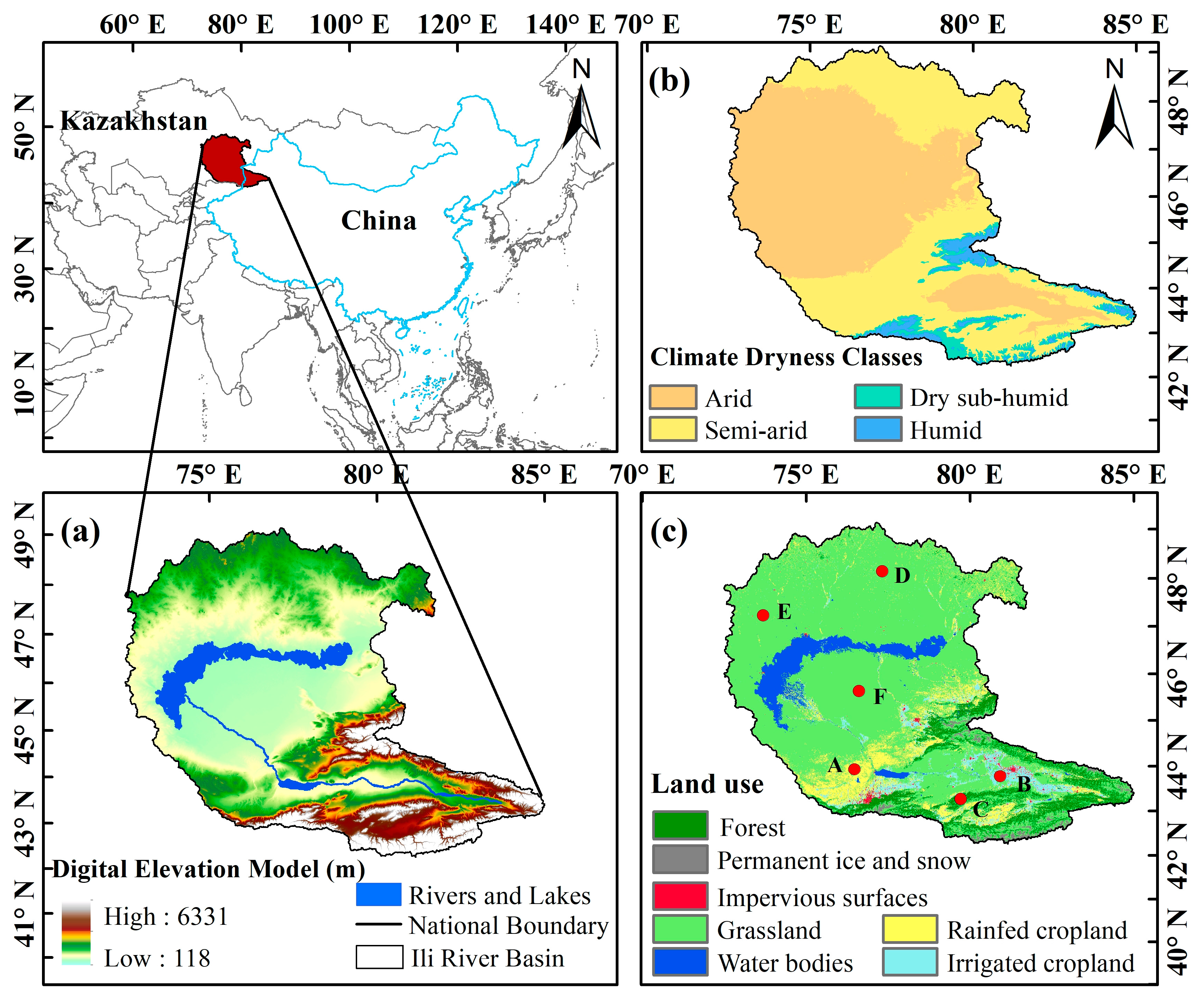
2.1. Study Area Description
2.2. Data Sources
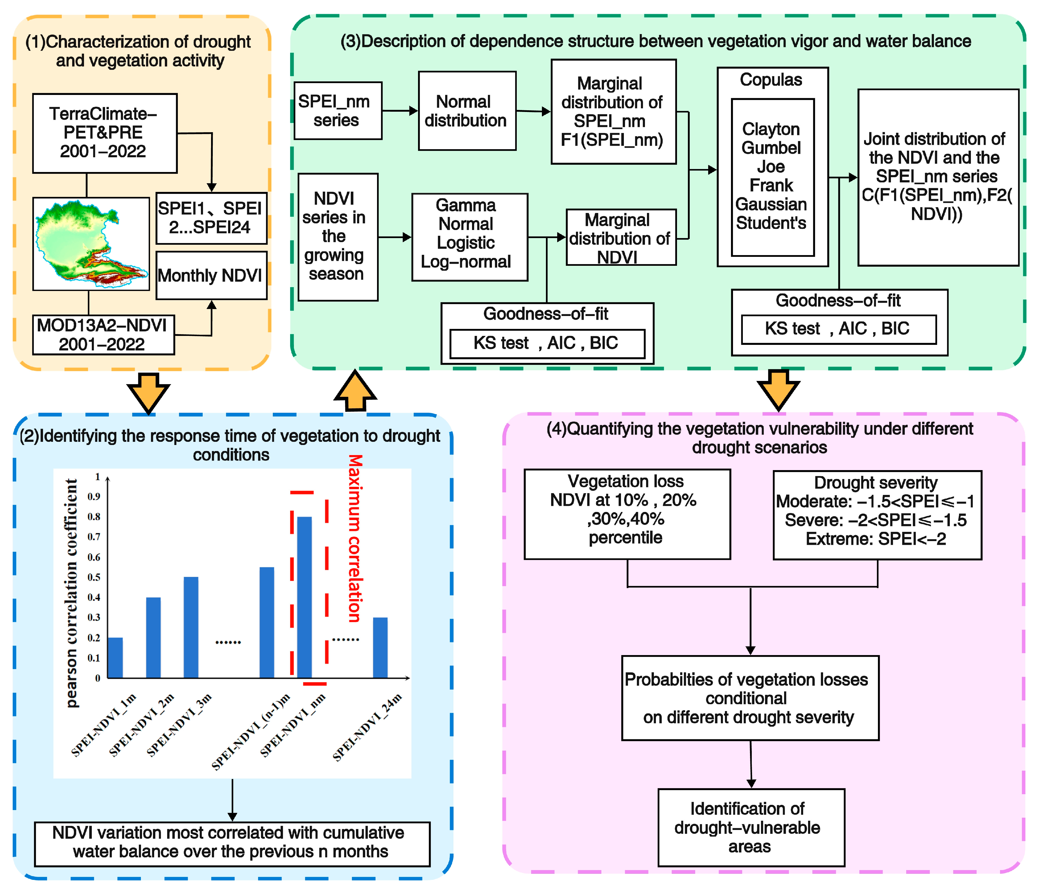
3. Methods
3.1. Standardized Precipitation Evapotranspiration Index
3.2. Correlation Among NDVI and SPEI
3.3. Copula Method to Quantify Vegetation Vulnerability
3.3.1. Copula
3.3.2. Assessment of Vegetation Loss Probability
4. Results
4.1. Sensitivity of Vegetation Dynamics to Water Deficits
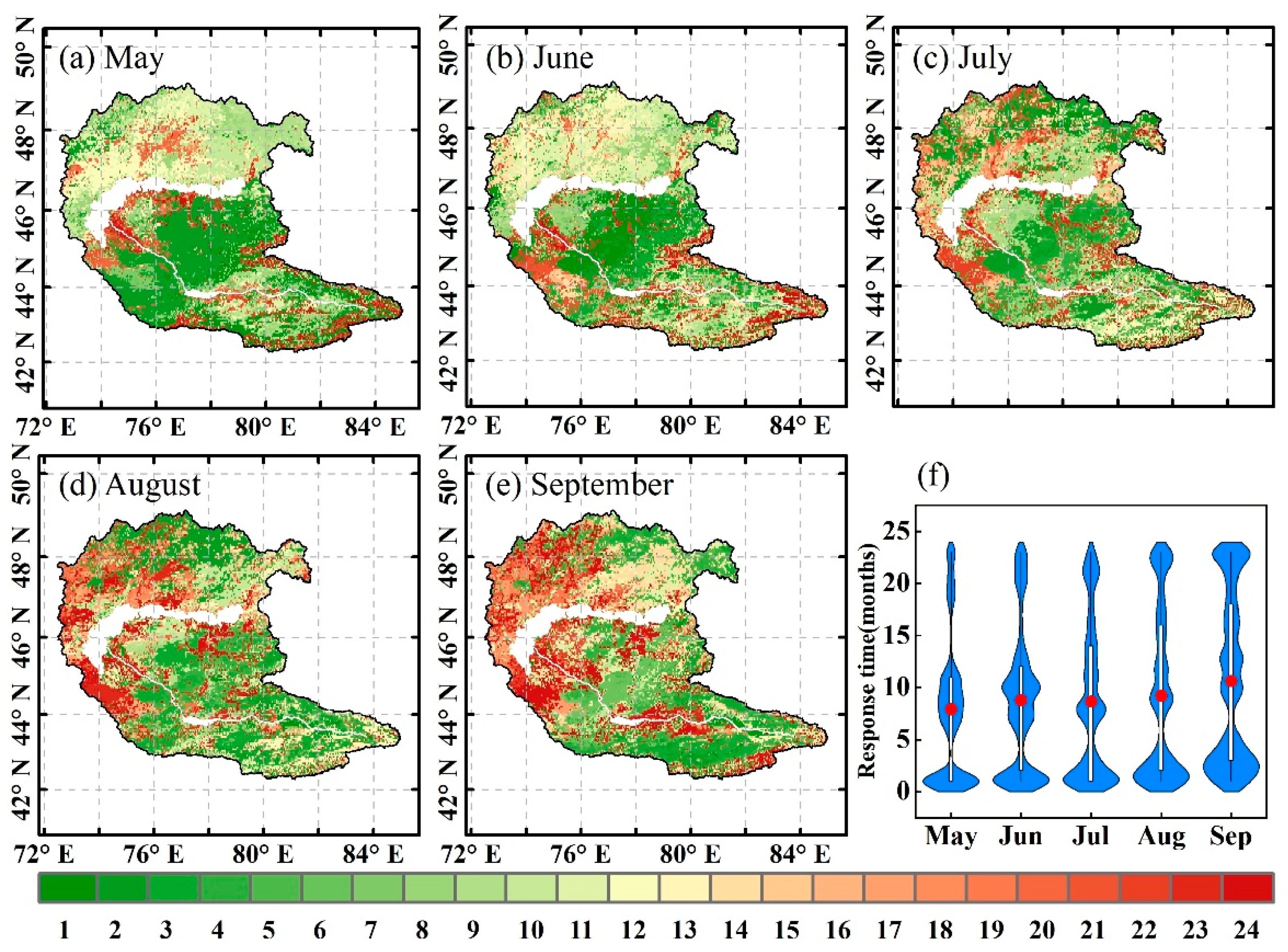
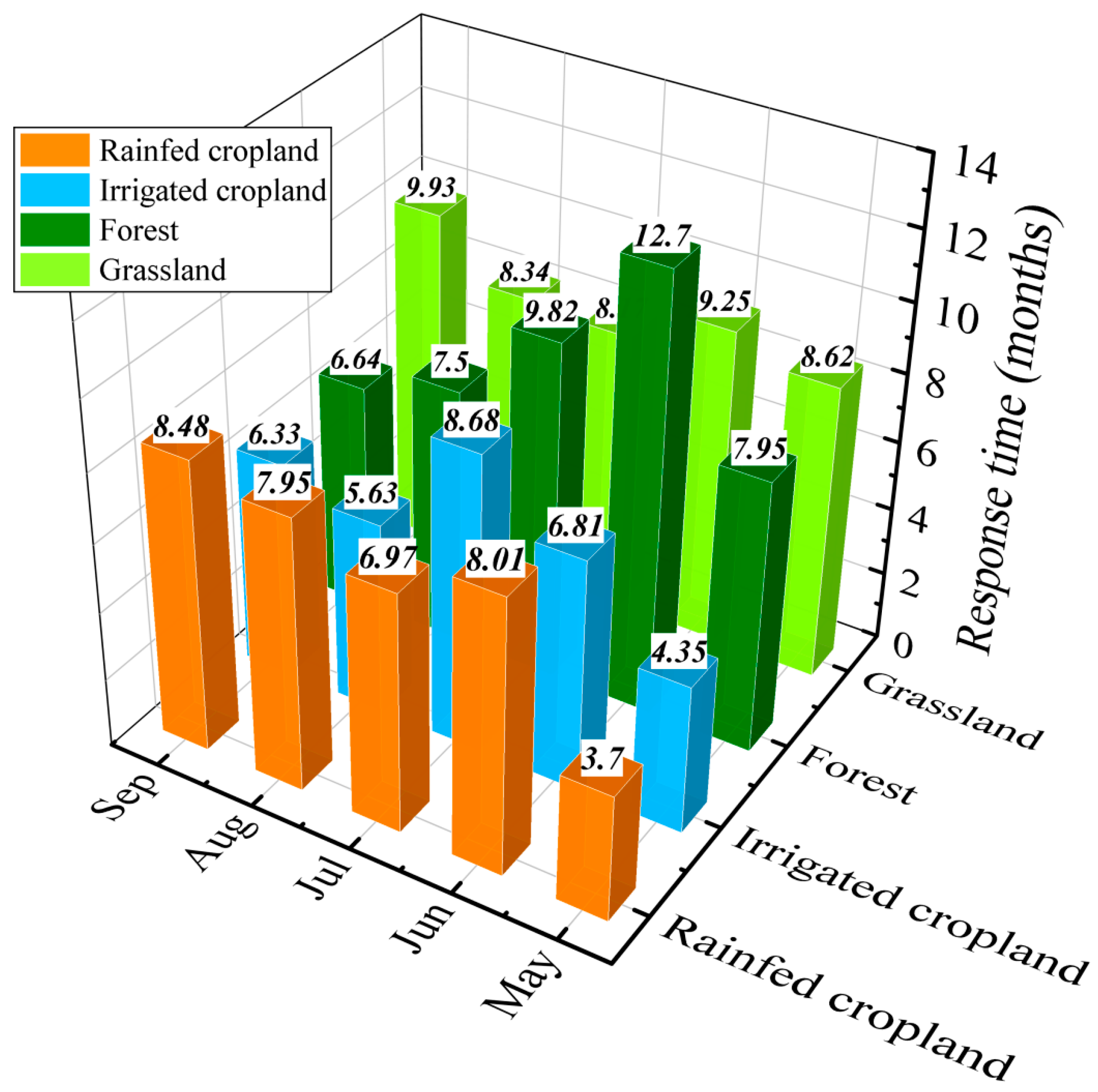
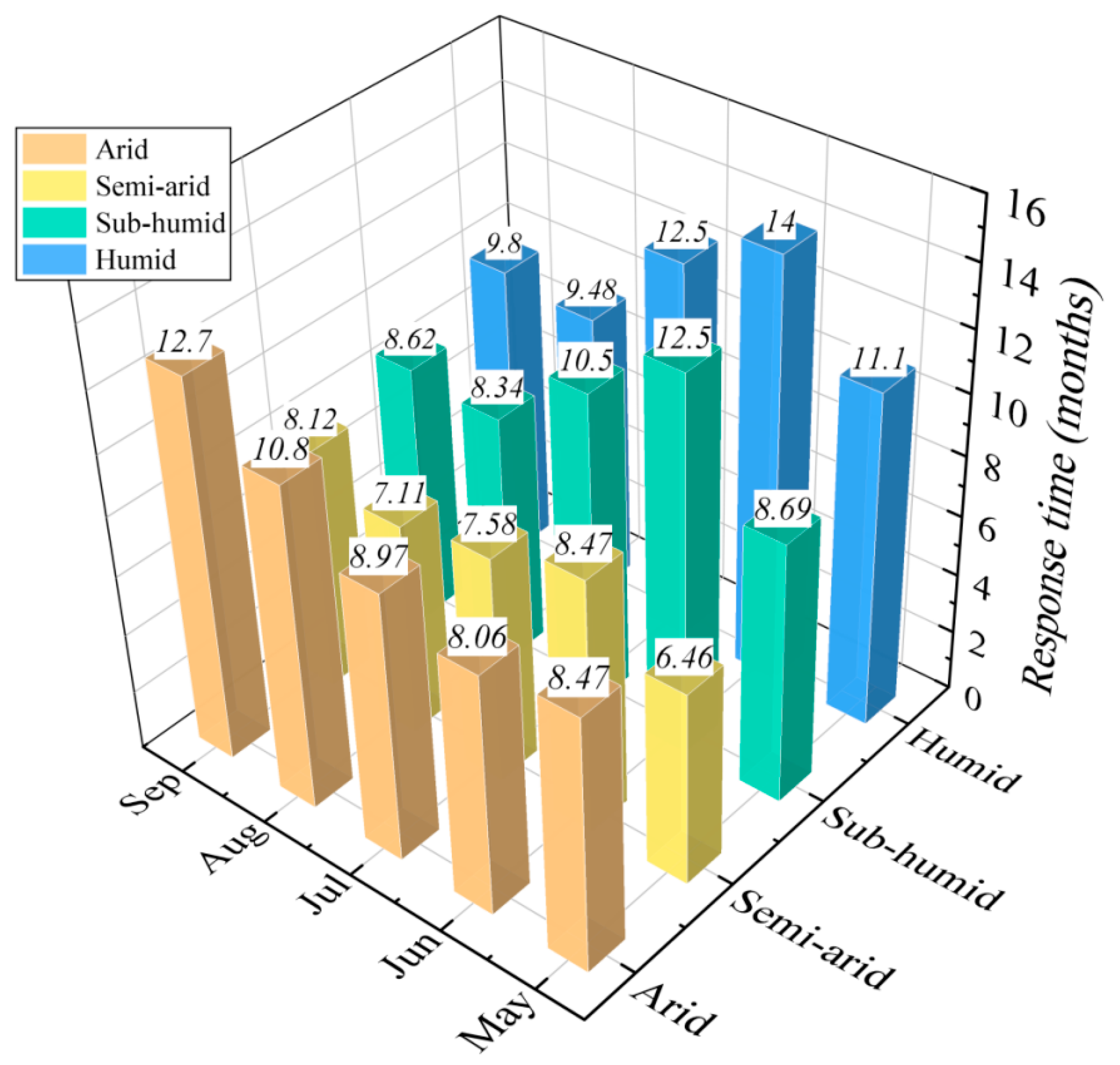
4.2. Response Time of Vegetation Dynamics to Water Deficits
4.3. Assessment of Vegetation Vulnerability
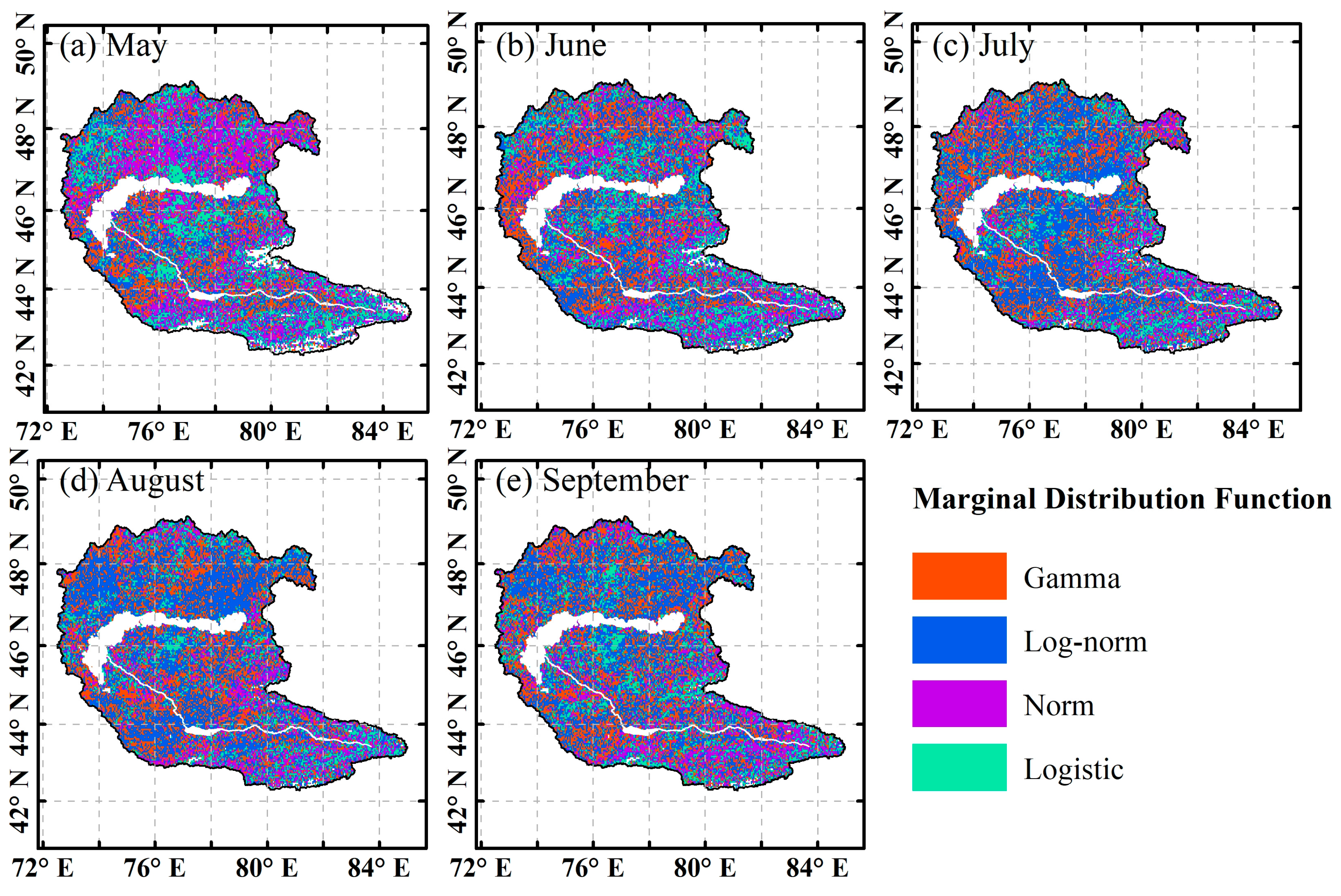
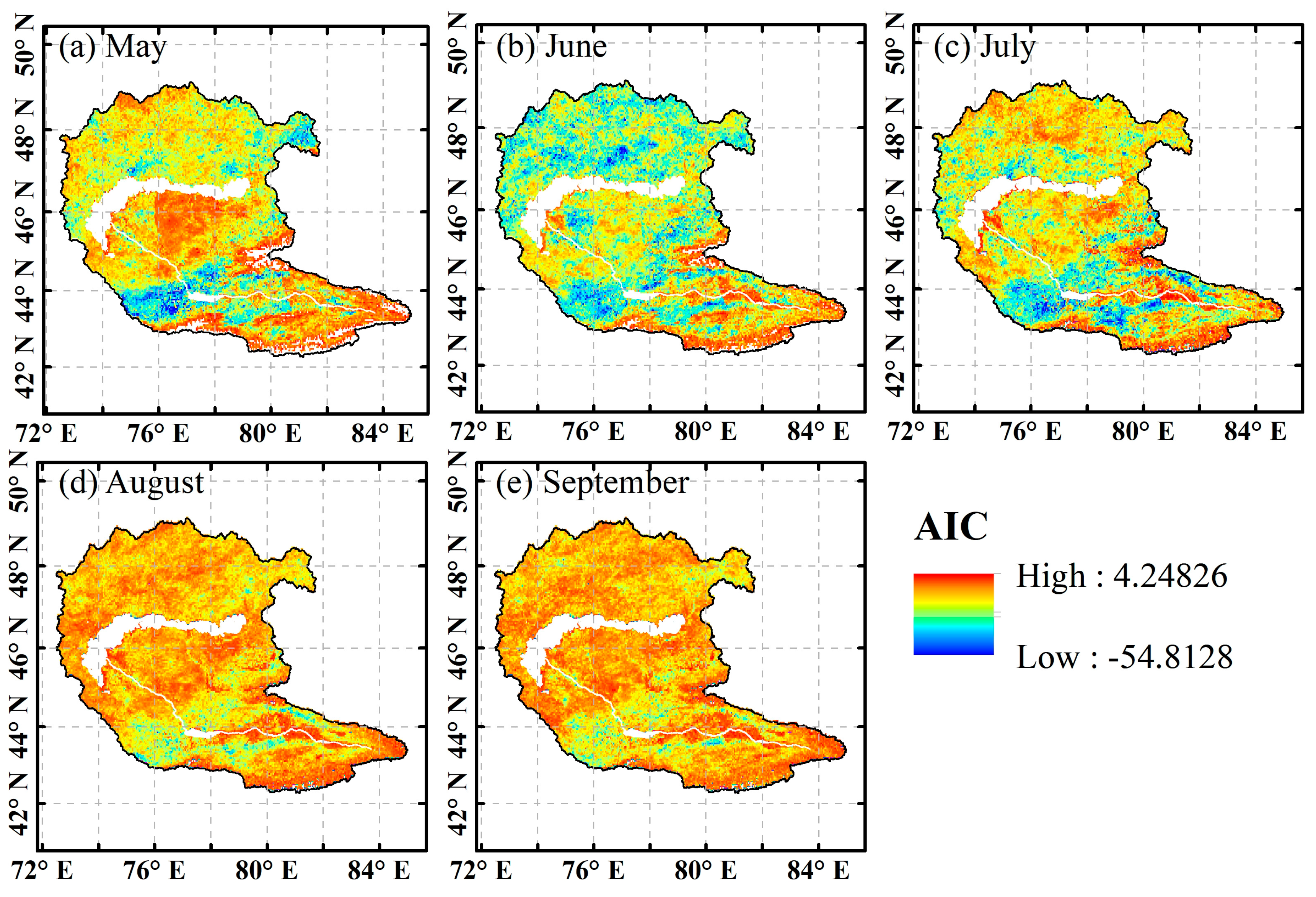
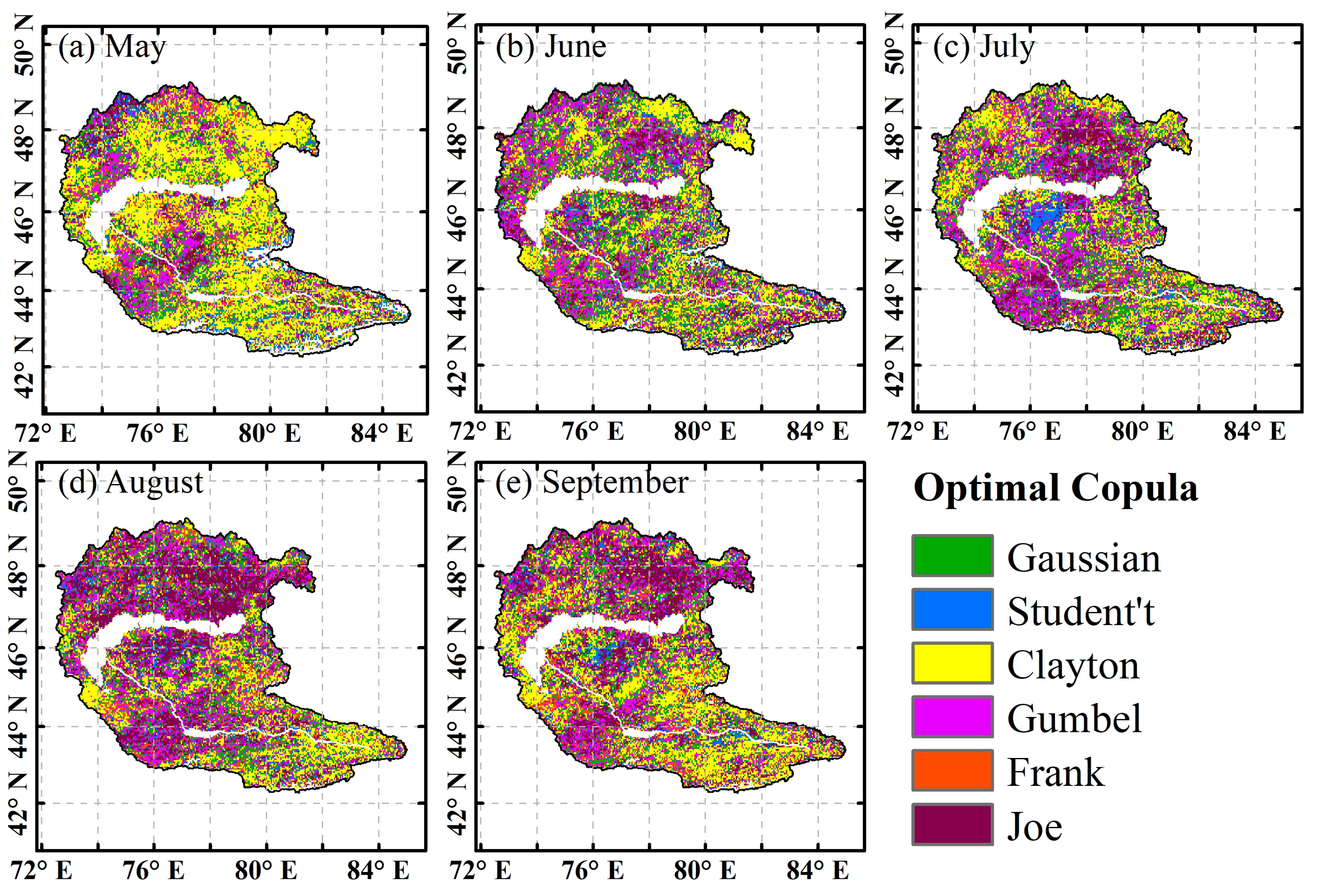
4.3.1. Reliability Validation of the Copula Model
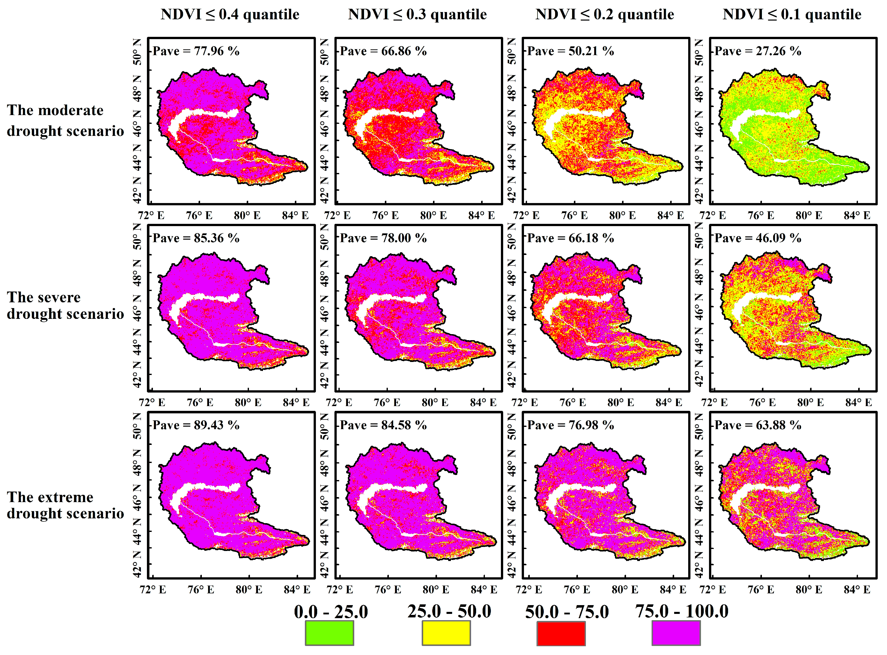
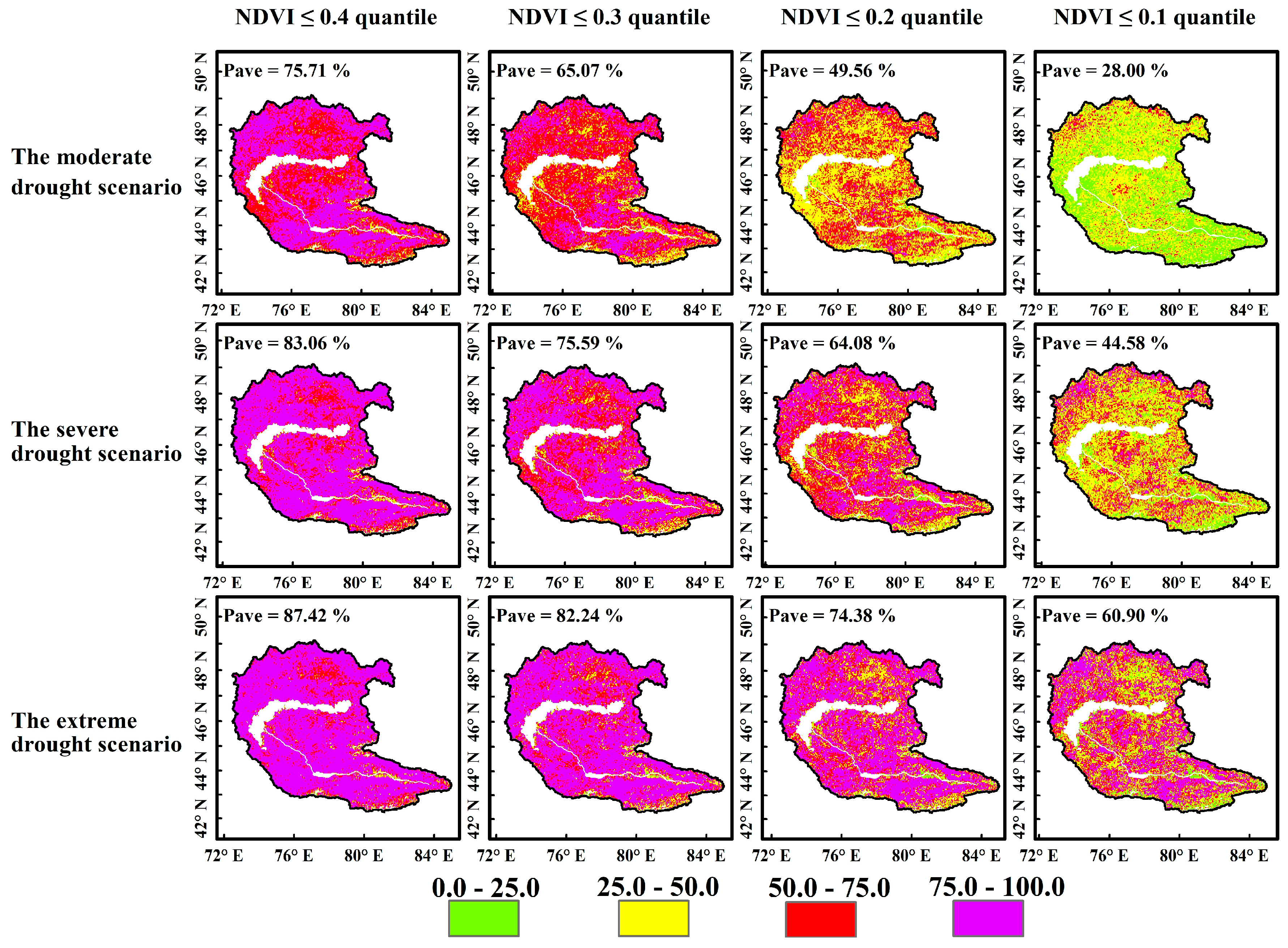
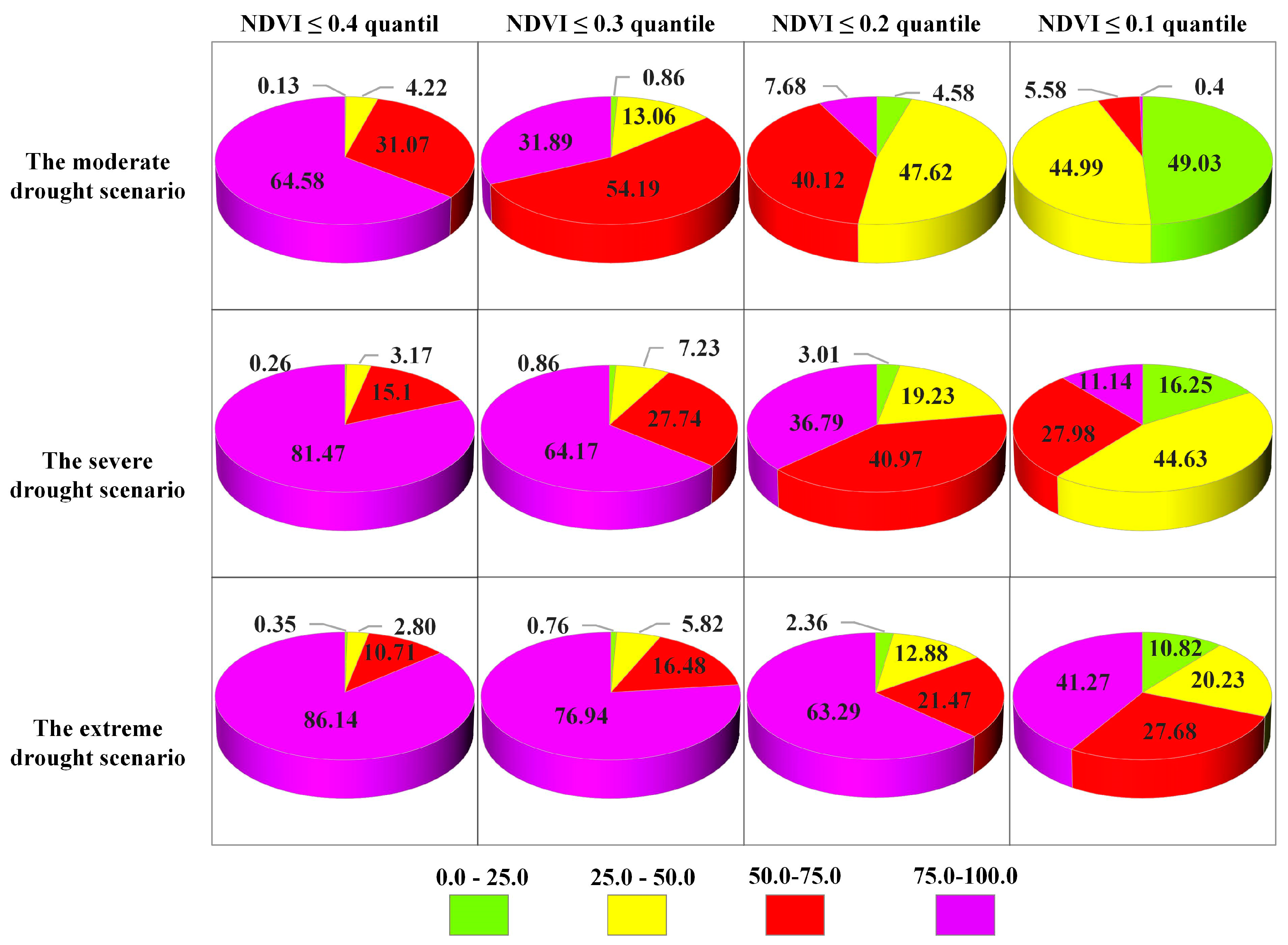
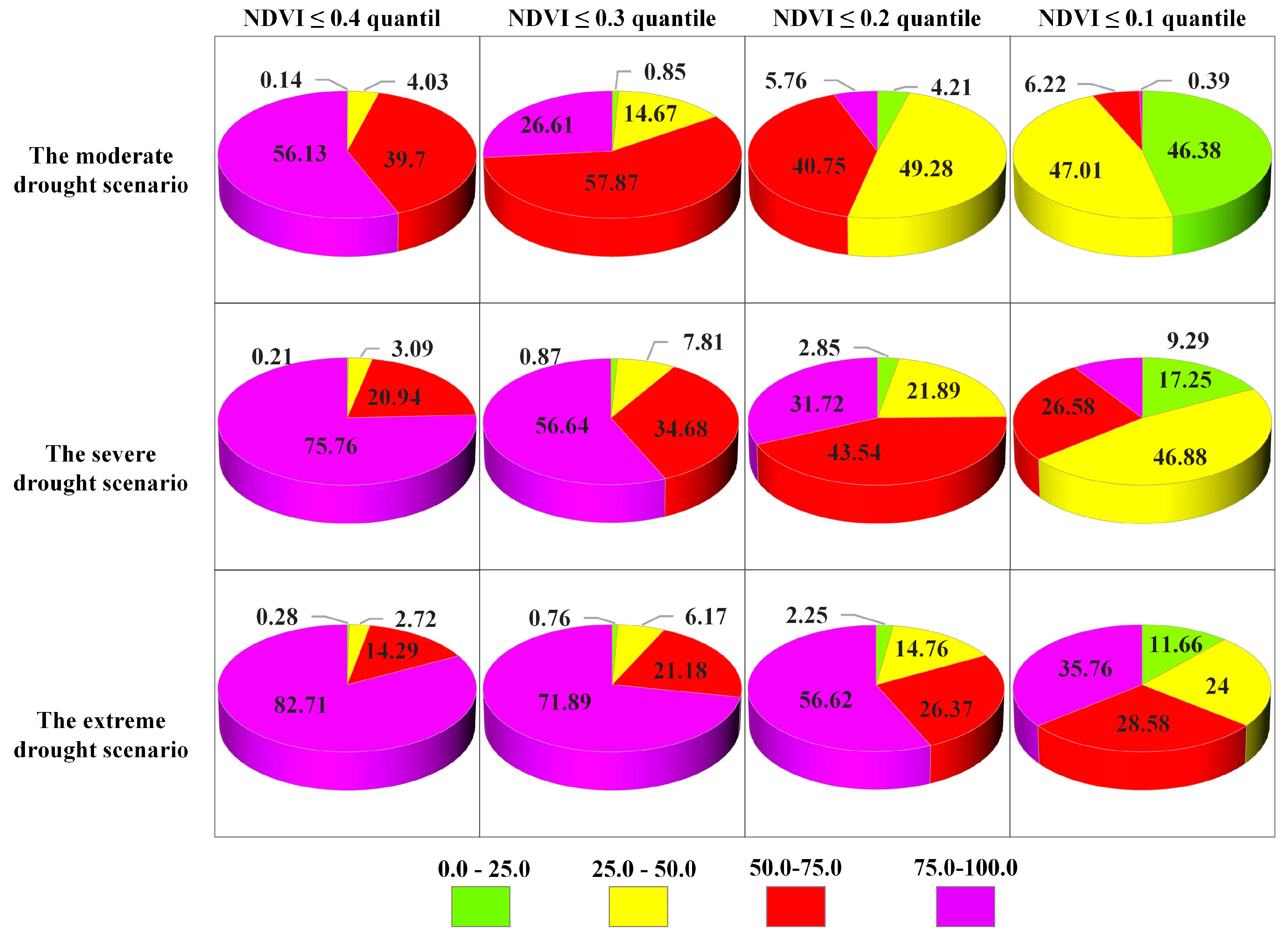
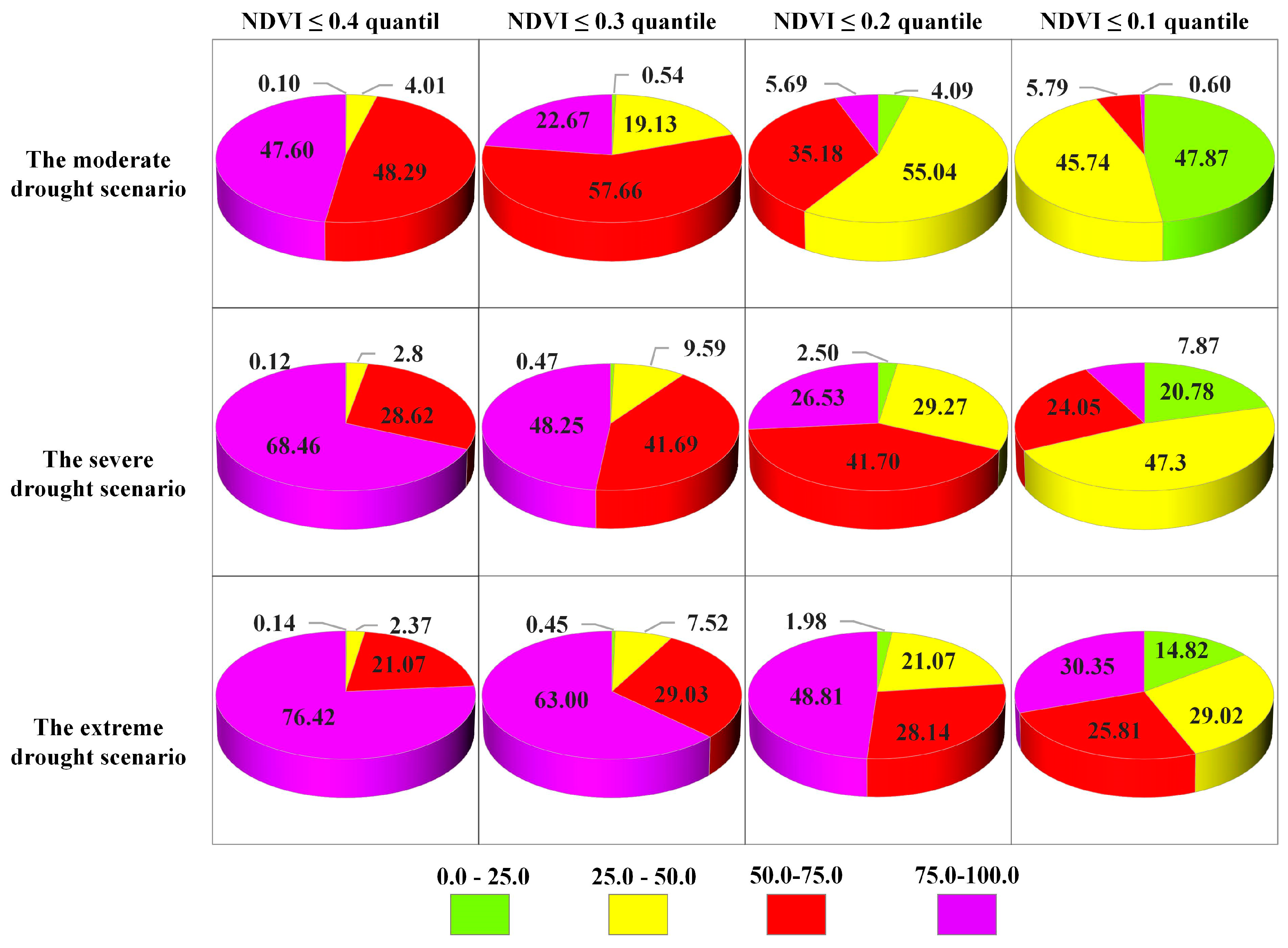
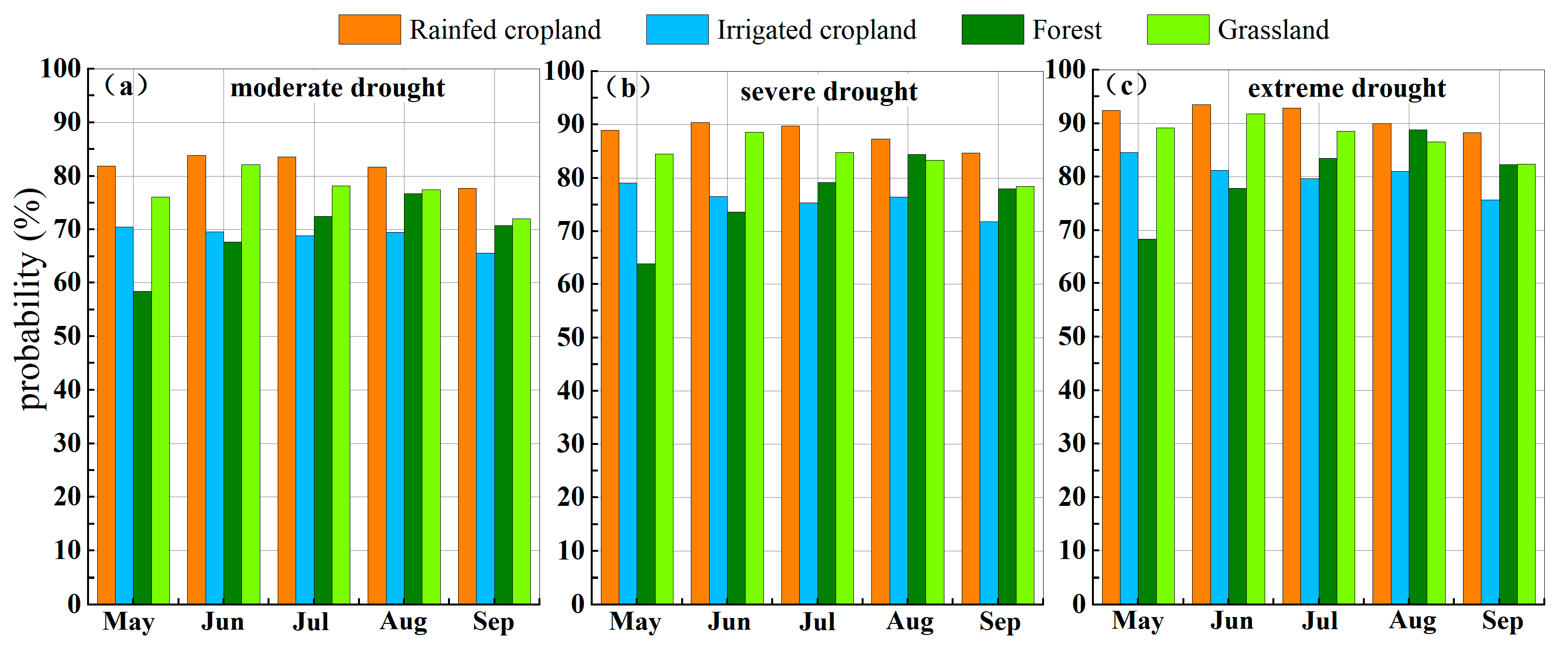
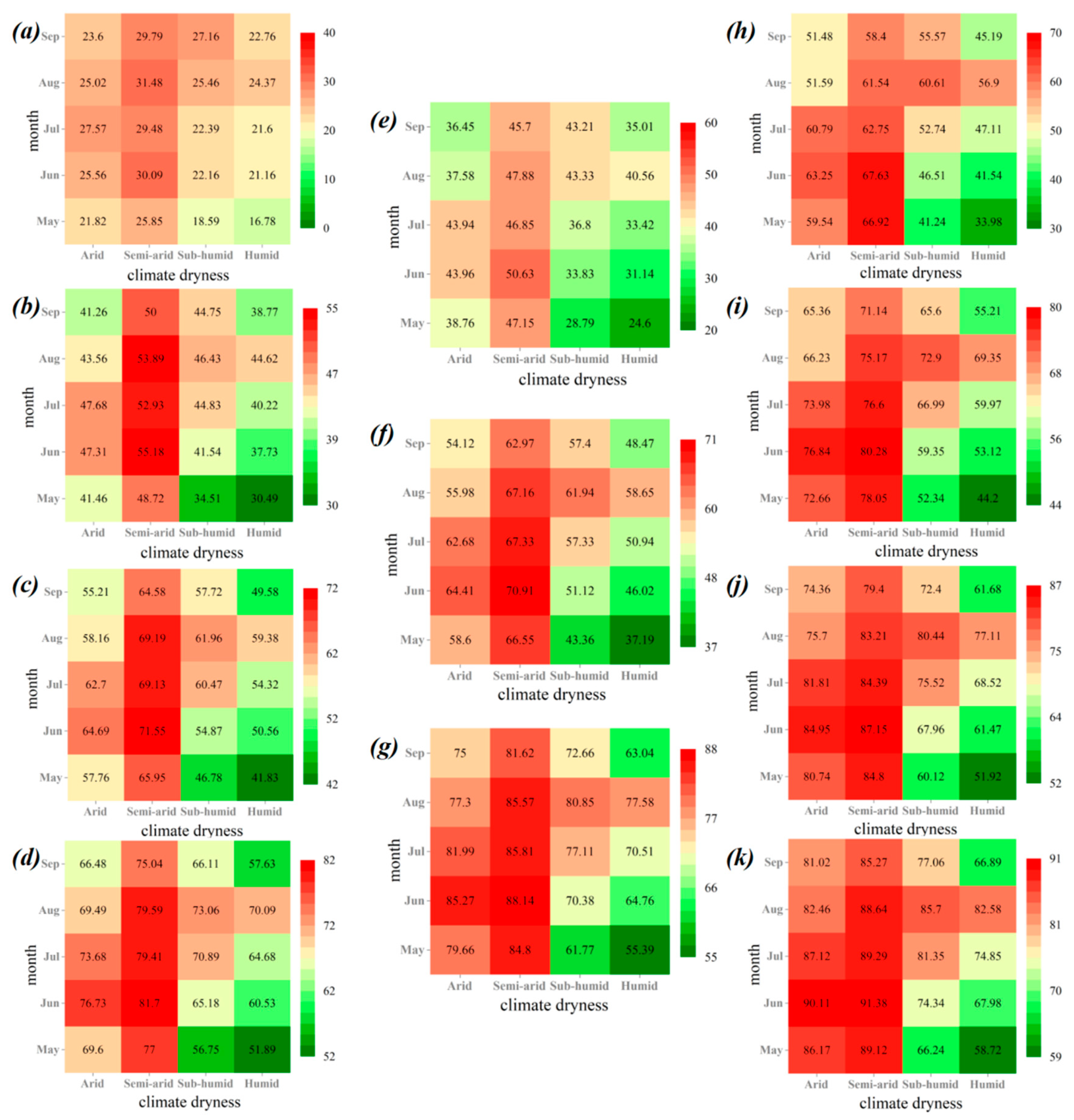
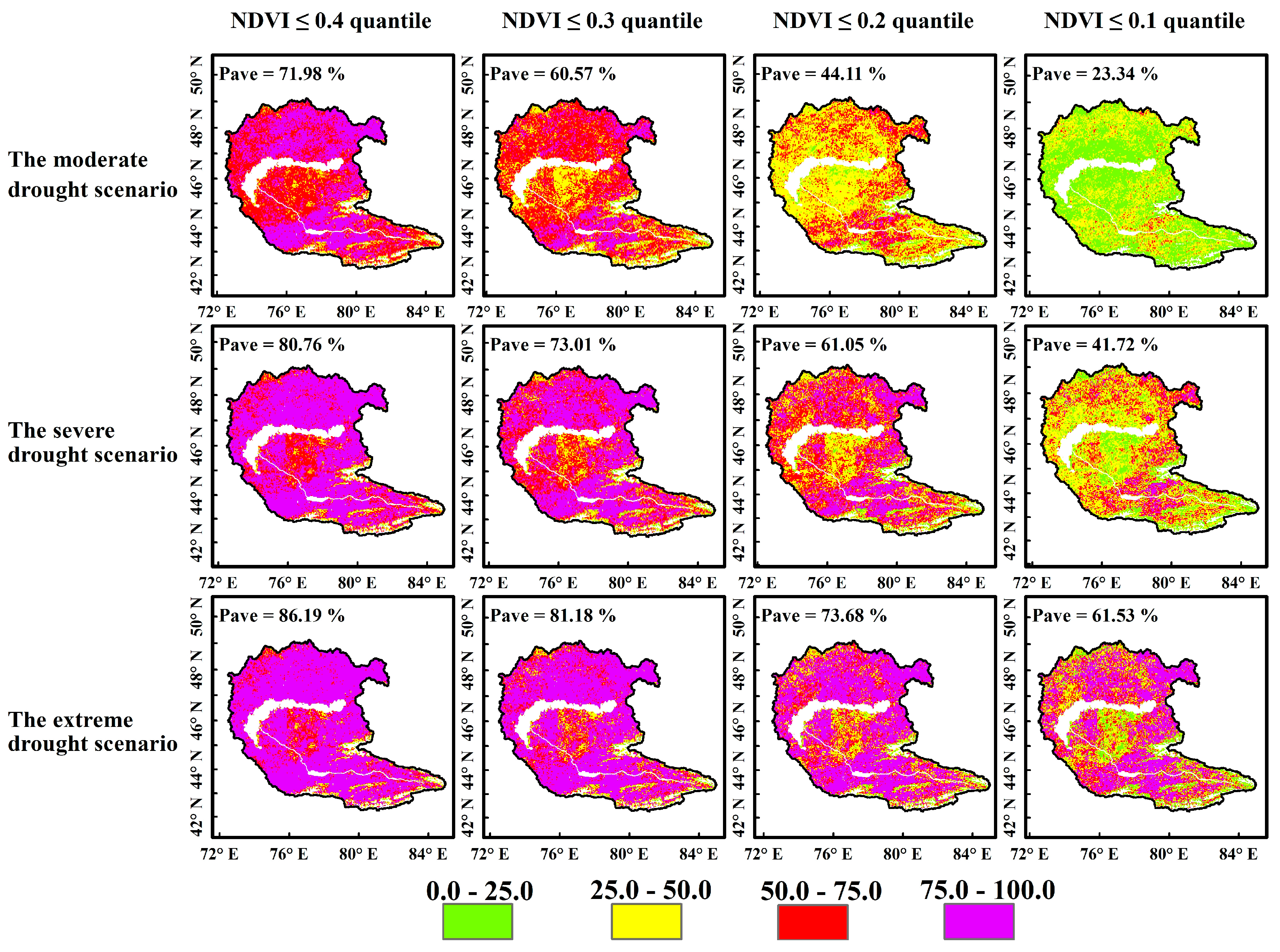
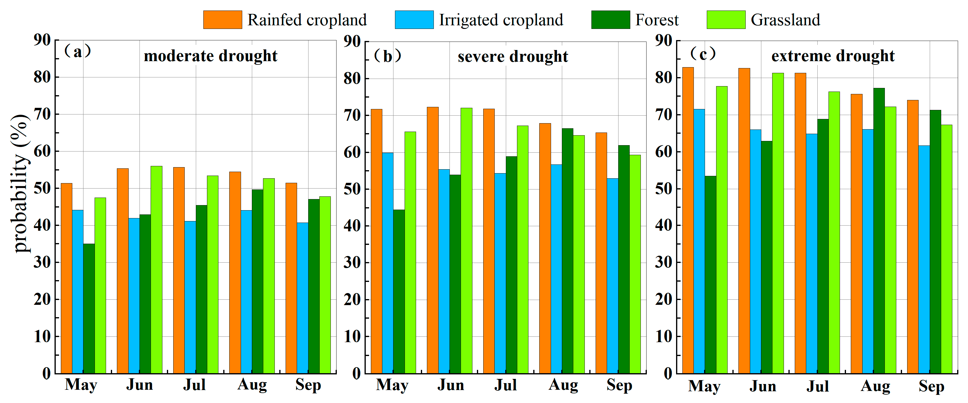
4.3.2. Probability of Vegetation Loss Under Different Drought Scenarios
5. Discussion
6. Conclusions
Author Contributions
Funding
Data Availability Statement
Conflicts of Interest
Appendix A


References
- IPCC. Climate Change 2021: The Physical Science Basis (Contribution of Working Group I to the Sixth Assessment Report of the Intergovernmental Panel on Climate Change); IPCC: Geneve, Switzerland, 2021. [Google Scholar]
- Li, H.; Li, Z.; Chen, Y.; Xiang, Y.; Liu, Y.; Kayumba, P.M.; Li, X. Drylands face potential threat of robust drought in the CMIP6 SSPs scenarios. Environ. Res. Lett. 2021, 16, 114004. [Google Scholar] [CrossRef]
- Guo, W.; Huang, S.; Huang, Q.; Leng, G.; Mu, Z.; Han, Z.; Wei, X.; She, D.; Wang, H.; Wang, Z. Drought trigger thresholds for different levels of vegetation loss in China and their dynamics. Agric. For. Meteorol. 2023, 331, 109349. [Google Scholar] [CrossRef]
- Lesk, C.; Anderson, W.; Rigden, A.; Coast, O.; Jägermeyr, J.; McDermid, S.; Davis, K.F.; Konar, M. Compound heat and moisture extreme impacts on global crop yields under climate change. Nat. Rev. Earth Environ. 2022, 3, 872–889. [Google Scholar] [CrossRef]
- Lindner, M.; Maroschek, M.; Netherer, S.; Kremer, A.; Barbati, A.; Garcia-Gonzalo, J.; Seidl, R.; Delzon, S.; Corona, P. Climate change impacts, adaptive capacity, and vulnerability of European forest ecosystems. For. Ecol. Manag. 2010, 259, 698–709. [Google Scholar] [CrossRef]
- Fang, W.; Huang, S.; Huang, Q.; Huang, G.; Wang, H.; Leng, G.; Wang, L.; Li, P.; Ma, L. Bivariate probabilistic quantification of drought impacts on terrestrial vegetation dynamics in mainland China. J. Hydrol. 2019, 577, 123980. [Google Scholar] [CrossRef]
- Yang, J.; Wu, J.; Liu, L.; Zhou, H.; Gong, A.; Han, X.; Zhao, W. Responses of winter wheat yield to drought in the North China Plain: Spatial–temporal patterns and climatic drivers. Water 2020, 12, 3094. [Google Scholar] [CrossRef]
- Liu, S.; Li, T.; Liu, B.; Xu, C.; Zhu, Y.; Xiao, L. Grassland vegetation decline is exacerbated by drought and can be mitigated by soil improvement in Inner Mongolia, China. Sci. Total Environ. 2024, 15, 168464. [Google Scholar] [CrossRef] [PubMed]
- Yang, J.; Li, Y.; Zhou, L.; Zhang, Z.; Zhou, H.; Wu, J. Effects of temperature and precipitation on drought trends in Xinjiang, China. J. Arid Land 2024, 16, 1098–1117. [Google Scholar] [CrossRef]
- Ding, Y.; Xu, J.; Wang, X.; Peng, X.; Cai, H. Spatial and temporal effects of drought on Chinese vegetation under different coverage levels. Sci. Total Environ. 2020, 716, 137166. [Google Scholar] [CrossRef]
- Liu, X.; Zhu, X.; Li, S.; Liu, Y.; Pan, Y. Changes in Growing Season Vegetation and Their Associated Driving Forces in China during 2001–2012. Remote Sens. 2015, 7, 15517–15535. [Google Scholar] [CrossRef]
- Jiang, L.; Jiapaer, G.; Bao, A.; Guo, H.; Ndayisaba, F. Vegetation dynamics and responses to climate change and human activities in Central Asia. Sci. Total Environ. 2017, 599–600, 967–980. [Google Scholar] [CrossRef] [PubMed]
- Qi, X.; Jia, J.; Liu, H.; Lin, Z. Relative importance of climate change and human activities for vegetation changes on China’s silk road economic belt over multiple timescales—ScienceDirect. Catena 2019, 180, 224–237. [Google Scholar] [CrossRef]
- Jin, H.; Vicente-Serrano, S.M.; Tian, F.; Cai, Z.; Conradt, T.; Boincean, B.; Murphy, C.; Farizo, B.A.; Grainger, S.; López-Moreno, J.I. Higher vegetation sensitivity to meteorological drought in autumn than spring across European biomes. Commun. Earth Environ. 2023, 4, 299. [Google Scholar] [CrossRef]
- Li, Y.; Dong, G.; Xue, H.; Zheng, Y.; Lian, Y. Effects of Multi-time Scale Meteorological Drought on Vegetation in the Yellow River Basin from 1982 to 2020. J. Soil Water Conserv. 2024, 38, 187–196. [Google Scholar]
- Poonia, V.; Jha, S.; Goyal, M.K. Copula based analysis of meteorological, hydrological and agricultural drought characteristics across Indian river basins. Int. J. Climatol. 2021, 41, 4637–4652. [Google Scholar] [CrossRef]
- Goswami, P.; Hazra, B.; Kumar, G. Copula-based probabilistic characterization of precipitation extremes over North Sikkim Himalaya. Atmos. Res. 2018, 212, 273–284. [Google Scholar] [CrossRef]
- Uttarwar, S.B.; Barma, S.D.; Mahesha, A. Bivariate Modeling of Hydroclimatic Variables in Humid Tropical Coastal Region Using Archimedean Copulas. J. Hydrol. Eng. 2020, 25, 05020026. [Google Scholar] [CrossRef]
- Nelsen Roger, B.; Quesada-Molina, J.J.; Rodríguez-Lallena, J.A.; Úbeda-Flores, M. Distribution functions of copulas: A class of bivariate probability integral transforms. Stat. Probab. Lett. 2001, 54, 277–282. [Google Scholar] [CrossRef]
- Kao, S.C.; Govindaraju, R.S. A copula-based joint deficit index for droughts. J. Hydrol. 2010, 380, 121–134. [Google Scholar] [CrossRef]
- Chen, L.; Singh, V.P.; Guo, S.L.; Mishra, A.K.; Guo, J. Drought Analysis Using Copulas. J. Hydrol. Eng. 2013, 18, 797–808. [Google Scholar] [CrossRef]
- Huang, S.; Hou, B.; Chang, J.; Huang, Q.; Chen, Y. Copulas-based probabilistic characterization of the combination of dry and wet conditions in the Guanzhong Plain, China. J. Hydrol. 2014, 519, 3204–3213. [Google Scholar] [CrossRef]
- Mirabbasi, R.; Fakheri-Fard, A.; Dinpashoh, Y. Bivariate drought frequency analysis using the copula method. Theor. Appl. Climatol. 2012, 108, 191–206. [Google Scholar] [CrossRef]
- Madadgar, S.; Aghakouchak, A.; Farahmand, A.; Davis, S.J. Probabilistic estimates of drought impacts on agricultural production. Geophys. Res. Lett. 2017, 44, 7799–7807. [Google Scholar] [CrossRef]
- Jha, S.; Das, J.; Sharma, A.; Hazra, B.; Goyal, M.K. Probabilistic evaluation of vegetation drought likelihood and its implications to resilience across India. Glob. Planet. Change 2019, 176, 23–25. [Google Scholar] [CrossRef]
- Han, F.; Ling, H.; Yan, J.; Deng, M.; Deng, X.; Gong, Y.; Wang, W. Shift in the migration trajectory of the green biomass loss barycenter in Central Asia. Sci. Total Environ. 2022, 847, 157656. [Google Scholar] [CrossRef] [PubMed]
- Muthuvel, D.; Sivakumar, B.; Mahesha, A. Future global concurrent droughts and their effects on maize yield. Sci. Total Environ. 2023, 855, 158860. [Google Scholar] [CrossRef] [PubMed]
- Wang, L.; Good, S.P.; Caylor, K.K. Global synthesis of vegetation control on evapotranspiration partitioning. Geophys. Res. Lett. 2014, 41, 6753–6757. [Google Scholar] [CrossRef]
- Yuan, W.; Piao, S.; Qin, D.; Dong, W.; Xia, J.; Lin, H.; Chen, M. Influence of vegetation growth on the enhanced seasonality of atmospheric CO2. Glob. Biogeochem. Cycle 2018, 32, 32–41. [Google Scholar] [CrossRef]
- Li, H.; Li, Y.; Huang, G.; Sun, J. Quantifying effects of compound dry-hot extremes on vegetation in Xinjiang (China) using a vine-copula conditional probability model. Agric. For. Meteorol. 2021, 311, 108658. [Google Scholar] [CrossRef]
- Li, H.; Li, Y.; Huang, G.; Sun, J. Probabilistic assessment of crop yield loss to drought time-scales in Xinjiang, China. Int. J. Climatol. 2021, 41, 4077–4094. [Google Scholar] [CrossRef]
- Han, W.; Guan, J.; Zheng, J.; Liu, Y.; Ju, X.; Liu, L.; Li, J.; Mao, X.; Li, C. Probabilistic assessment of drought stress vulnerability in grasslands of Xinjiang, China. Front. Plant Sci. 2023, 14, 1143863. [Google Scholar] [CrossRef]
- Li, Z.; Zheng, F.; Liu, W.; Flanagan, D.C. Spatial distribution and temporal trends of extreme temperature and precipitation events on the Loess Plateau of China during 1961–2007. Quat. Int. 2010, 226, 92–100. [Google Scholar] [CrossRef]
- Trabucco, A.; Zomer, R. Global aridity index and potential evapotranspiration (ET0) climate database v2. CGIAR Consort. Spat. Inf. 2018, 10, m9. [Google Scholar]
- Monteith; Lennox, J. Evaporation and environment. Symp. Soc. Exp. Biol. 1965, 19, 205–234. [Google Scholar] [PubMed]
- Borgomeo, E.; Pflug, G.; Hall, J.W.; Hochrainer-Stigler, S. Assessing water resource system vulnerability to unprecedented hydrological drought using copulas to characterize drought duration and deficit. Water Resour. Res. 2015, 51, 8927–8948. [Google Scholar] [CrossRef] [PubMed]
- Campos-Taberner, M.; Moreno-Martínez, Á.; García-Haro, F.J.; Camps-Valls, G.; Robinson, N.P.; Kattge, J.; Running, S.W. Global Estimation of Biophysical Variables from Google Earth Engine Platform. Remote Sens. 2018, 10, 1167. [Google Scholar] [CrossRef]
- Guo, Y.; Huang, S.; Huang, Q.; Wang, H.; Fang, W. Copulas-based bivariate socioeconomic drought dynamic risk assessment in a changing environment. J. Hydrol. 2019, 575, 1052–1064. [Google Scholar] [CrossRef]
- Sadegh, M.; Ragno, E.; Aghakouchak, A. Multivariate Copula Analysis Toolbox (MvCAT): Describing dependence and underlying uncertainty using a Bayesian framework. Water Resour. Res. 2017, 53, 5166–5183. [Google Scholar] [CrossRef]
- Fang, W.; Huang, S.; Huang, Q.; Huang, G.; Wang, H.; Leng, G.; Wang, L.; Li, P.; Ma, L. Probabilistic assessment of remote sensing-based terrestrial vegetation vulnerability to drought stress of the Loess Plateau in China. Remote Sens. Environ. 2019, 232, 111290. [Google Scholar] [CrossRef]
- Chen, T.; Tang, G.; Yuan, Y.; Guo, H.; Xu, Z.; Jiang, G.; Chen, X. Unraveling the relative impacts of climate change and human activities on grassland productivity in Central Asia over last three decades. Sci. Total Environ. 2020, 743, 140649. [Google Scholar] [CrossRef]
- Anderegg, W.R.L.; Schwalm, C.; Biondi, F.; Camarero, J.J.; Koch, G.; Litvak, M.; Ogle, K.; Shaw, J.D.; Shevliakova, E.; Williams, A.P. Pervasive drought legacies in forest ecosystems and their implications for carbon cycle models. Science 2015, 349, 528–532. [Google Scholar] [CrossRef] [PubMed]
- Wen, Y.; Liu, X.; Xin, Q.; Wu, J.; Xu, X.; Pei, F.; Li, X.; Du, G.; Cai, Y.; Lin, K. Cumulative Effects of Climatic Factors on Terrestrial Vegetation Growth. J. Geophys. Res.-Biogeosci. 2019, 124, 789–806. [Google Scholar] [CrossRef]
- Zhu, S.; Xiao, Z.; Luo, X.; Zhang, H.; Huo, Z. Multidimensional Response Evaluation of Remote-Sensing Vegetation Change to Drought Stress in the Three-River Headwaters, China. IEEE J. Sel. Top. Appl. Earth Observ. Remote Sens. 2020, 13, 6249–6259. [Google Scholar] [CrossRef]
- Zou, J.; Ding, J.; Welp, M.; Huang, S.; Liu, B. Using MODIS data to analyse the ecosystem water use efficiency spatial-temporal variations across Central Asia from 2000 to 2014. Environ. Res. 2020, 182, 108985. [Google Scholar] [CrossRef]
- Yang, Y.; Guan, H.; Batelaan, O.; Simmons, C. Contrasting response of water use efficiency to drought across global terrestrial ecosystems. Sci. Rep. 2016, 6, 23284. [Google Scholar] [CrossRef]
- Lundholm, B. Adaptations in arid ecosystems. Ecol. Bull. 1976, 24, 19–27. [Google Scholar]
- Schwinning, S.; Sala, O.E. Hierarchy of responses to resource pulses in arid and semi-arid ecosystems. Oecologia 2004, 141, 211–220. [Google Scholar] [CrossRef] [PubMed]
- Van der Molen, M.K.; Dolman, A.J.; Ciais, P.; Eglin, T.; Gobron, N.; Law, B.E.; Meir, P.; Peters, W.; Phillips, O.L.; Reichstein, M. Drought and ecosystem carbon cycling. Agric. For. Meteorol. 2011, 151, 765–773. [Google Scholar] [CrossRef]
- Li, F.; Zhang, M.; Zhao, Y.; Jiang, R. Influence of irrigation and groundwater on the propagation of meteorological drought to agricultural drought. Agric. Water Manag. 2023, 277, 108099. [Google Scholar]
- Sperry, J.S. Hydraulic constraints on plant gas exchange. Agric. For. Meteorol. 2000, 104, 13–23. [Google Scholar] [CrossRef]
- Shi, M.; Yuan, Z.; Shi, X.; Li, M.; Chen, F.; Li, Y. Drought assessment of terrestrial ecosystems in the Yangtze River Basin, China. J. Clean. Prod. 2022, 362, 132234. [Google Scholar] [CrossRef]
- Abatzoglou, J.T.; Dobrowski, S.Z.; Parks, S.A.; Hegewisch, K.C. Data Descriptor: TerraClimate, a high-resolution global dataset ofmonthly climate and climatic water balance from 1958–2015. Sci. Data 2018, 5, 170191. [Google Scholar] [CrossRef]
- Alimaev, I.; Kerven, C.; Torekhanov, A.; Behnke, R.; Smailov, K.; Yurchenko, V.; Sisatov, Z.; Shanbaev, K. The Impact of Livestock Grazing on Soils and Vegetation Around Settlements in Southeast Kazakhstan: South Kazakhstan Pasture Use Results; Springer: Berlin/Heidelberg, Germany, 2008; pp. 81–112. [Google Scholar]
- Guan, X.; Shen, H.; Li, X.; Gan, W.; Zhang, L. A long-term and comprehensive assessment of the urbanization-induced impacts on vegetation net primary productivity. Sci. Total Environ. 2019, 669, 342–352. [Google Scholar] [CrossRef]
- Bowman, D.M.J.S.; Kolden, C.A.; Abatzoglou, J.T.; Johnston, F.H.; Van Der Werf, G.R.; Flannigan, M. Vegetation fires in the Anthropocene. Nat. Rev. Earth Environ. 2020, 1, 500–515. [Google Scholar] [CrossRef]
- Hao, Y.; Hao, Z.; Fu, Y.; Feng, S.; Zhang, X.; Wu, X.; Hao, F. Probabilistic assessments of the impacts of compound dry and hot events on global vegetation during growing seasons. Environ. Res. Lett. 2021, 16, 074055. [Google Scholar] [CrossRef]
- Heimann, M.; Reichstein, M. Terrestrial ecosystem carbon dynamics and climate feedbacks. Nature 2008, 451, 289–292. [Google Scholar] [CrossRef] [PubMed]
- Jiang, J.; Zhou, T.; Chen, X.; Zhang, L. Future changes in precipitation over Central Asia based on CMIP6 projections. Environ. Res. Lett. 2020, 15, 054009. [Google Scholar] [CrossRef]


| Drought Level | SPEI Value |
|---|---|
| No drought | SPEI > −0.5 |
| Light drought | −1.0 < SPEI ≤ −0.5 |
| Moderate drought | −1.5 < SPEI ≤ −1.0 |
| Severe drought | −2.0 < SPEI ≤ −1.5 |
| Extreme drought | SPEI ≤ −2.0 |
Disclaimer/Publisher’s Note: The statements, opinions and data contained in all publications are solely those of the individual author(s) and contributor(s) and not of MDPI and/or the editor(s). MDPI and/or the editor(s) disclaim responsibility for any injury to people or property resulting from any ideas, methods, instructions or products referred to in the content. |
© 2025 by the authors. Licensee MDPI, Basel, Switzerland. This article is an open access article distributed under the terms and conditions of the Creative Commons Attribution (CC BY) license (https://creativecommons.org/licenses/by/4.0/).
Share and Cite
Li, Y.; Yang, J.; Wu, J.; Zhang, Z.; Xia, H.; Ma, Z.; Gao, L. Spatiotemporal Responses and Vulnerability of Vegetation to Drought in the Ili River Transboundary Basin: A Comprehensive Analysis Based on Copula Theory, SPEI, and NDVI. Remote Sens. 2025, 17, 801. https://doi.org/10.3390/rs17050801
Li Y, Yang J, Wu J, Zhang Z, Xia H, Ma Z, Gao L. Spatiotemporal Responses and Vulnerability of Vegetation to Drought in the Ili River Transboundary Basin: A Comprehensive Analysis Based on Copula Theory, SPEI, and NDVI. Remote Sensing. 2025; 17(5):801. https://doi.org/10.3390/rs17050801
Chicago/Turabian StyleLi, Yaqian, Jianhua Yang, Jianjun Wu, Zhenqing Zhang, Haobing Xia, Zhuoran Ma, and Liang Gao. 2025. "Spatiotemporal Responses and Vulnerability of Vegetation to Drought in the Ili River Transboundary Basin: A Comprehensive Analysis Based on Copula Theory, SPEI, and NDVI" Remote Sensing 17, no. 5: 801. https://doi.org/10.3390/rs17050801
APA StyleLi, Y., Yang, J., Wu, J., Zhang, Z., Xia, H., Ma, Z., & Gao, L. (2025). Spatiotemporal Responses and Vulnerability of Vegetation to Drought in the Ili River Transboundary Basin: A Comprehensive Analysis Based on Copula Theory, SPEI, and NDVI. Remote Sensing, 17(5), 801. https://doi.org/10.3390/rs17050801