An Extension of Ozone Profile Retrievals from TROPOMI Based on the SAO2024 Algorithm

Abstract

We investigate the retrieval of ozone (O₃) profiles, with a particular focus on tropospheric O₃, from backscattered ultraviolet radiances measured by the TROPOspheric Monitoring Instrument (TROPOMI), using the UV2 (300–332 nm) and UV3 (305–400 nm) channels independently. An optimal estimation retrieval algorithm, originally developed for the Ozone Monitoring Instrument (OMI), was extended as a preliminary step toward integrating multiple satellite ozone profile datasets. The UV2 and UV3 channels exhibit distinct radiometric and wavelength calibration uncertainties, leading to inconsistencies in retrieval accuracy and convergence stability. A yearly “soft” calibration mitigates overestimation and cross-track-dependent biases (“stripes”) in tropospheric ozone retrievals, enhancing retrieval consistency between UV2 and UV3. Convergence stability is ensured by optimizing the measurement error constraints for each channel. It is shown that our research product outperforms the standard product (UV1 and UV2 combined) in capturing the seasonal and long-term variabilities of tropospheric ozone. An agreement between the retrieved tropospheric ozone and ozonesonde measurements is observed within 0–3 DU ± 5.5 DU (R = 0.75), which is better than that of the standard product by a factor of two. Despite lacking Hartley ozone information in UV2 and UV3, the retrieved stratospheric ozone columns have good agreement with ozonesondes (R = 0.96).

1. Introduction

Ozone plays a crucial role in protecting and influencing the environment depending on its location in the atmosphere. The ozone layer in the stratosphere protects life from the sun’s harmful ultraviolet (UV) radiation, whereas ground-level ozone has detrimental effects on living organisms, including humans, animals, and plants [1,2,3]. In the middle and upper troposphere, ozone is the third most important anthropogenic greenhouse gas, after carbon dioxide and methane [4].

Satellite measurements of backscattered ultraviolet (BUV) radiance have been regularly used to measure the global total column ozone and vertical profiles of ozone in the Earth’s atmosphere for half a century since NASA’s Nimbus-7 satellite was launched in 1978 with Total Ozone Monitoring Spectrometer (TOMS) and Solar Backscatter Ultraviolet Radiometer (SBUV) instruments [5]. Since Bhartia et al. (1985) [6] showed the first satellite image confirming the Antarctic ozone hole phenomenon, continuous ozone layer monitoring has been one of the primary objectives of satellite missions. The first space-borne observation of ozone profiles down to the troposphere was made using the Global Ozone Monitoring Experiment (GOME) instrument, thanks to its hyperspectral capability of capturing the fine absorption features of ozone over a wide range of the spectrum [7]. Inverse schemes have been robustly developed and established to retrieve ozone profiles using GOME hyperspectral measurements [8,9,10,11,12]. Significant progress has been made in instrument design, from the GOME to its successor, the Ozone Monitoring Instrument (OMI), launched in July 2004 onboard the Aura spacecraft, with the capability of detecting urban-scale variations with daily global coverage [13]. In particular, OMI exhibits unprecedented long-term stability in radiometric and wavelength calibrations but is approaching the end of its mission. By focusing on the ozone layer, the measurement series of the total ozone column is continued by the Ozone Mapping and Profiler Suite (OMPS) instruments onboard the joint NASA/NOAA Suomi National Polar-orbiting Partnership (Suomi NPP) and Joint Polar Satellite System (JPSS) satellites [14,15]. Launched in October 2017 by the European Space Agency (ESA), the Sentinel-5 Precursor (S5P) spacecraft plays a crucial role in monitoring trace gases and aerosols related to air quality and climate [16]. Onboard, the TROPOspheric Monitoring Instrument (TROPOMI) follows the heritage of OMI in instrument design but has advantages such as finer spatial resolution, higher signal-to-noise ratio, and wider spectral coverage. The TROPOMI observations have shown good agreement with OMI, demonstrating better performance in detecting localized hotspots of trace gases and aerosols [17,18]. The 5 years of operational TROPOMI ozone profile data were evaluated against ozonesonde and lidar measurements, reporting a 5–10% agreement in the troposphere and −5% in the upper stratosphere with ±2% drifts per year [19]. In addition, ozone profile retrieval was independently investigated by An et al. (2024), Mettig et al. (2021), and Zhao et al. (2021) [20,21,22]. These retrievals involve the iterative fitting of spectral observations to their forward model simulation with either a priori constraints or regularization to stabilize the retrieval state. The optimal estimation (OE) approach [23], which relies on a priori constraints based on ozone profile climatology, has been incorporated into most of the aforementioned studies. The first-order Tikhonov regularization approach [24], which combines an a priori constraint with an altitude-independent smoothness constraint, was employed by Mettig et al. (2021) [21].

This study aims to adapt and extend the OE-based Smithsonian Astrophysical Observatory (SAO) ozone profile algorithm [10,25,26] as a primary step toward the synergistic integration of reliable ozone profiles from OMI and TROPOMI measurements. OMI Collection 3 L1B data were processed to create the OMI ozone profile product using an earlier version of the SAO algorithm, referred to as the SAO2010 algorithm. This OMI research product is publicly available, along with the OMI standard product [27]. The SAO2010 algorithm was improved to reprocess the OMI Collection 4 data, with updates improving the calibration model, forward model, and auxiliary datasets, and is referred to as the SAO2024 algorithm [25]. Zhao et al. (2021) [22] examined Version 1 of the L1B TROPOMI data using the SAO2010 algorithm for ozone profile retrieval. In this study, the SAO2024 algorithm is employed with improved L1B version 2.1 TROPOMI data in bands 1–3 (UV1, UV2, and UV3) (See

Table 1. Characteristics of TROPOMI spectral bands 1 and 2 in UV and band 3 in UVN.

Band ID	1	2	3
Spectral range (nm)	267–300	300–332	305–400
Spectral resolution (nm)	0.45–0.5		0.45–0.65
Spectral sampling (nm)	0.065		0.195
Along-track ground pixel size (km) +	5.5	5.5	5.5
Across-track ground pixel size (km) @	28···60	3.5···15	3.5···15
Binning factor *	4···16	1···2	1···2
Spatial dimension #	77	448	450
Minimal Signal-to-noise ratio	50	50–600	100–1200

⁺ Along-track pixel size: Initially 7 km, improved to 5.5 km as of 6 August 2019. ^@ Across-track pixel size: varies significantly from the center (smaller) and the edges (larger). * Higher binning factors are used at the center and reduced by half at the edges to obtain a more constant ground pixel size across-track. ^# The given value represents the number of cross-track pixels (detector rows). The number of wavelengths is 497 for all the bands (detector columns).

). The UV1 band contains the Hartley ozone band, whereas the spectral coverage of the UV1 and UV2 bands overlaps with that of the Huggins ozone band. Most of the aforementioned studies combined UV1 and UV2 to complete the fitting window of 270–330 nm, which allows for ozone profiling in both the troposphere and stratosphere without exploring the use of UV3 [19,20,21]. On the other hand, Zhao et al. (2021) [22] recommended using UV3 with version 1 spectral products for the best-quality tropospheric ozone products, owing to radiometric offsets in UV1 and radiometric noise in UV2.

The remainder of this paper is organized as follows. Section 2 describes the data used to retrieve and evaluate the ozone profiles. Section 3 details the retrieval methodology, focusing on re-calibrating radiometric and wavelength measurements. Section 4 compares ozone profile retrievals due to different radiometric accuracies in UV2 and UV3 bands. Moreover, retrieved ozone profiles are validated using ozonesonde soundings, with a cross-evaluation of the TROPOMI standard product (Section 5). Section 6 summarizes our conclusions.

2. Data

2.1. TROPOMI L1B Product

The S5P satellite is in a Sun-synchronous polar orbit at an altitude of 824 km, with an equatorial crossing at 13:30 local solar time on the ascending node. The single-payload TROPOMI is a nadir-viewing passive-grating imaging spectrometer. It operates in push-broom mode with a wide swath of approximately 2600 km on the Earth’s surface, achieving global coverage each day at a spatial resolution of 3.5 × 5.5 km². This instrument is equipped with four different spectrometers that measure both solar irradiance and the Earth’s radiance in the ultraviolet (UV 270–330 nm), visible (VIS 310–500 nm), near-infrared (NIR 675–775 nm), and shortwave infrared (SWIR 2305–2385 nm) regions. UV, VIS, and NIR spectrometers employ a two-dimensional charge-coupled device (CCD), with one dimension for wavelength and the other dimension for cross-track spatial coverage. Each detector is divided into two halves, resulting in a total of eight spectral bands. Spectral bands 1–3, summarized in Table 1, were used to retrieve the ozone profiles. We refer to bands 1–3 as UV1, UV2, and UV3. By correcting for temporal (degradation) effects in radiance and irradiance, as well as UVN gain drifts in the earlier data, version 2.1 of the L0-1B processor also introduces new flagging for “transient”, “blooming”, and “thermal instability” [28]. The reprocessed L1B data products used in this paper are available for the full operational phase (30 April 2018, until the present).

2.2. TROPOMI Standard Ozone Profile Product

The ESA/Copernicus Atmospheric Mission Performance Cluster (ATM-MPC) officially produces the ozone profile product through the processing chain of the L0 to L1B processor (version 2.1) and the optimal estimation-based L1B to L2 processor (version 2.4.0 and higher), as documented at https://sentiwiki.copernicus.eu/web/s5p-products (accessed on 12 February 2025). The retrieval processor uses bands 1 and 2, which are both recorded by the same UV detector but at different spatial resolutions [19]. To merge the data into a continuous spectrum of 270–330 nm, the 450 across-track pixels of the band 2 data are binned into 77 pixels to match the band 1 ground pixels. Merged UV spectra are averaged over five consecutive scan lines. The resulting product has a spatial resolution of 28 × 28 km (across-track × along-track) at the nadir after 6 August 2019 and 28 × 35 km² before that date, which is an improvement over the OMI standard ozone profile product (48 × 65 km²) [27]. To account for the remaining calibration uncertainties, the irradiance wavelength registration is corrected for a shift relative to the Fraunhofer lines, and a yearly radiometric correction is applied to the Sun-normalized radiance. The spectral simulation is based on the DISAMAR software [29]. The a priori ozone profiles are taken from the climatology of [30], which consists of the average ozone profiles as a function of the total ozone for six 30° latitude bands. The a priori error is primarily based on the standard deviations (20–50%) of the ozone profile climatology but is fixed at 50% in the troposphere below 250 hPa. The retrieved ozone profiles are provided as number densities at 33 levels (mole/m³). In this study, TROPOMI standard ozone profiles were used for cross-evaluation along with our research ozone profiles.

2.3. Ozonesondes

The satellite retrievals were evaluated using electrochemical concentration cell (ECC) ozonesonde observations collected at the five stations listed in

Table 2. Lists of ozonesonde stations.

Station	Country	Lon, Lat (°)	Elevation (m)	Launch time (LT) #	Provider
Ascension Island	UK	14.22W, 7.56S	85	12:30	SHADOZ 1
King’s Park	Hong Kong	114.17E, 22.31N	66	13:30	WOUDC 2
Pohang	South Korea	129.37E, 36.03N	2.5	14:00	KMA 3
Tsukuba	Japan	140.13E, 36.06N	31	14:30	WOUDC
Lindenberg	Germany	14.1E, 52.2N	112	12:00	WOUDC

^# The median local time of balloon launches. ¹ Southern Hemisphere ADditional OZonesondes (SHADOZ) project. ² World Ozone and Ultraviolet Radiation Data Centre (WOUDC). ³ Korea Meteorological Administration (KMA).

. At these stations, ozonesondes were routinely launched weekly without major interruptions during the validation period from 2018 to 2023. These launches typically occurred in the afternoon (12:00–14:30 LT). In this study, individual ozonesonde soundings were spatiotemporally co-located to the TROPOMI ozone profiles within a 100 km radius and a 6 h window, after which the spatially closest pair was selected. As a result, the collocated pairs were identified within a distance of 14.8 ± 10 km and a time difference of 1–3 h. To enhance validation accuracy, ozonesonde measurements were excluded if the tropospheric ozone column was abnormally high (>80 DU), the stratospheric ozone column was abnormally low (<100 DU), the balloon burst prematurely before reaching 200 hPa, or gaps exceeding 3 km were present in the profile data. The TROPOMI standard profiles were rejected if the quality flag (qa value) was less than 0.5, which typically occurs when the cost function is large or when the retrieved ozone significantly deviates from the a priori ozone [31]. The ozone profiles presented in this paper were validated if the retrieval converges within 10 iterations and the retrieved value is positive across all layers.

3. Retrieval Methodology

The SAO2024 algorithm was extended to retrieve ozone profiles from TROPOMI satellite observations. The algorithm implementation details remain unchanged from OMI to TROPOMI, which are briefly described in this section but are explained in great detail in Bak et al. (2024) [25]. Section 3.1 describes the general elements of the ozone profile algorithm. The rest of this section gives full details of the new features implemented to make the best use of TROPOMI measurements.

3.1. Heritage from SAO Ozone Profile Algorithm

The algorithm iteratively estimates the state vector variables ($\widehat{\mathit{X}}$) with the goal of minimizing the spectral residuals between the measured ($\mathit{Y}$) and simulated ($\mathit{R}$) radiances. Simultaneously, a priori (${\mathit{X}}_a$) is incorporated to constrain the retrieval state, depending on the a priori covariance matrix (${\mathbf{S}}_a$) and measurement error covariance matrix (${\mathbf{S}}_y)$. The a posteriori solution and cost function are expressed as

$${\widehat{\mathit{X}}}_{\mathrm{i}+1}={\widehat{\mathit{X}}}_i+{\left({\mathit{K}}_i^T{\mathbf{S}}_y^{-1}{\mathbf{K}}_i{+\mathbf{S}}_a^{-1}\right)}^{-1}\left[{\mathbf{K}}_i^T{\mathbf{S}}_y^{-1}\right(\mathit{Y}-\mathit{R}\left({\widehat{\mathit{X}}}_{\mathrm{i}}\right))-{\mathbf{S}}_a^{-1}({\widehat{\mathit{X}}}_i-{\mathit{X}}_a\left)\right]$$

(1)

$${\chi }^2={‖{\mathbf{S}}_y^{-\frac{1}{2}}\{{\mathbf{K}}_i\left({\widehat{\mathit{X}}}_{\mathrm{i}+1}-{\widehat{\mathit{X}}}_{\mathrm{i}}\right)-[\mathit{Y}-\mathit{R}({\widehat{\mathit{X}}}_{\mathrm{i}})]\})‖}_2^2+{‖{\mathbf{S}}_a^{-\frac{1}{2}}({\widehat{\mathit{X}}}_{\mathrm{i}+1}-{\mathit{X}}_a)‖}_2^2$$

(2)

where K is the weighing function matrix (∂R/∂$\widehat{\mathit{X}}$), composed of derivatives of the forward model with respect to an element of the state vector. The convergence criterion remains the same as in the OMI algorithm, ensuring that the relative change in the cost function value between consecutive iterations is less than 1.0%. To prevent divergence, the maximum number of iterations was set to 10.

The state vector consists of 33 elements, including three types of geophysical variables: partial ozone columns in 24 layers, wavelength-dependent surface albedo (first-order polynomial), and cloud fraction. It also includes two wavelength-shift variables (radiance/irradiance and radiance/ozone cross-section) and four other pseudo-absorbers to account for the ring effect, intensity offset, and changes in slit parameter (slit width and shape factor used to determine the super Gaussian shape). Note that common modes are fitted as pseudo-absorbers to account for the remaining residuals in OMI spectral fitting. However, including common modes was not effective in addressing TROPOMI spectral residuals and has therefore been excluded.

An a priori ozone profile is sampled from tropopause-based ozone profile climatology [32]. The a priori error covariance matrix is constructed with a correlation length of 6 km for the ozone profile. The measurement vector is composed of Sun-normalized radiances (ratio of radiance to irradiance). The forward model simulation was performed using principal component analysis (PCA)-vector linearized discrete ordinate radiative transfer (VLIDORT) with a lower-accuracy configuration for acceleration [33]. The decreased accuracy is compensated for by lookup table correction up to the level attainable from simulations using a vector model with 12 streams and 72 layers.

Each diagonal element of ${\mathbf{S}}_y$ is the sum of the squared random noise errors obtained from the L1B radiance and irradiance products. However, the resulting measurement constraints are typically underestimated. Therefore, the floor noise level is imposed to maintain a balance between the information content and retrieval stability. The retrieval experiment is presented in Section 3.2.4 to suggest floor values for UV2 and UV3. The cloud parameters are taken from the operational cloud product Optical Cloud Recognition Algorithm/Retrieval of Cloud Information using Neural Networks) [34]. This includes cloud top pressure, based on absorption by the O₂ A-band at 760 nm (in NIR) and effective cloud fraction, based on the radiative effect of clouds in the 350–390 nm (in UV3). We note that the discrepancy in cloud information at wavelengths used in the cloud and ozone retrieval algorithms is partly accounted for by including cloud fraction as a state vector, fitted along with ozone profile during the iterative retrieval process.

3.2. Optimization of TROPOMI Measurements

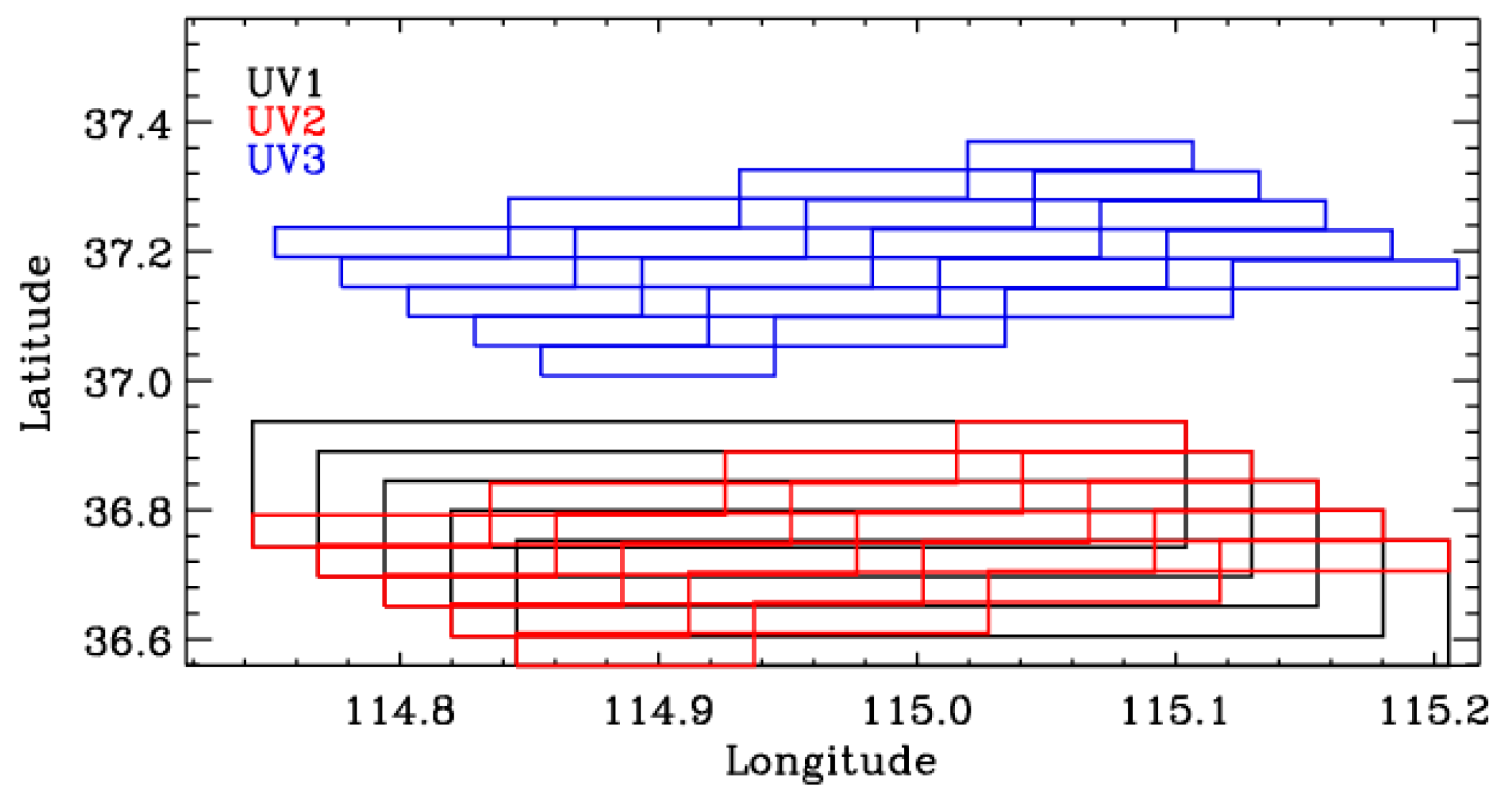
3.2.1. Spatial and Spectral Co-Adding

All three UV channels (bands 1–3) have different spatial samples. The cross-track pixels of UV1 are much coarser than those of UV2 and UV3 by a factor of four to eight, as specified in Table 1. By applying spatial bunning, UV2 can be matched exactly to UV1. The geolocations and geometries of UV2 and UV3 are slightly different (Figure 1) because they are measured by independent spectrometers.

To reduce the computational burden and compare the ozone profile retrievals with different UV channels, the ground pixels of both UV2 and UV3 were spatially binned into 77 cross-track pixels, matching the spatial resolution of UV1. In addition, all three channels were binned into five scan lines along the flight direction. The resulting spatial resolution is 28 km (across-track) × 28/35 km (along-track, before/after 6 August 2019) in the nadir, which matches that of the TROPOMI standard ozone profile product.

The spectral resolution in the UV channels ranges from 0.45 to 0.65 nm. However, the spectra are unnecessarily oversampled at intervals of 0.065 nm in UV1 and UV2. According to the Nyquist theorem, the information content can be mostly preserved with a sampling rate equal to half the spectral resolution. To address this, three consecutive wavelengths were averaged, resulting in a sampling rate of 0.195 nm, which is similar to that of UV3.

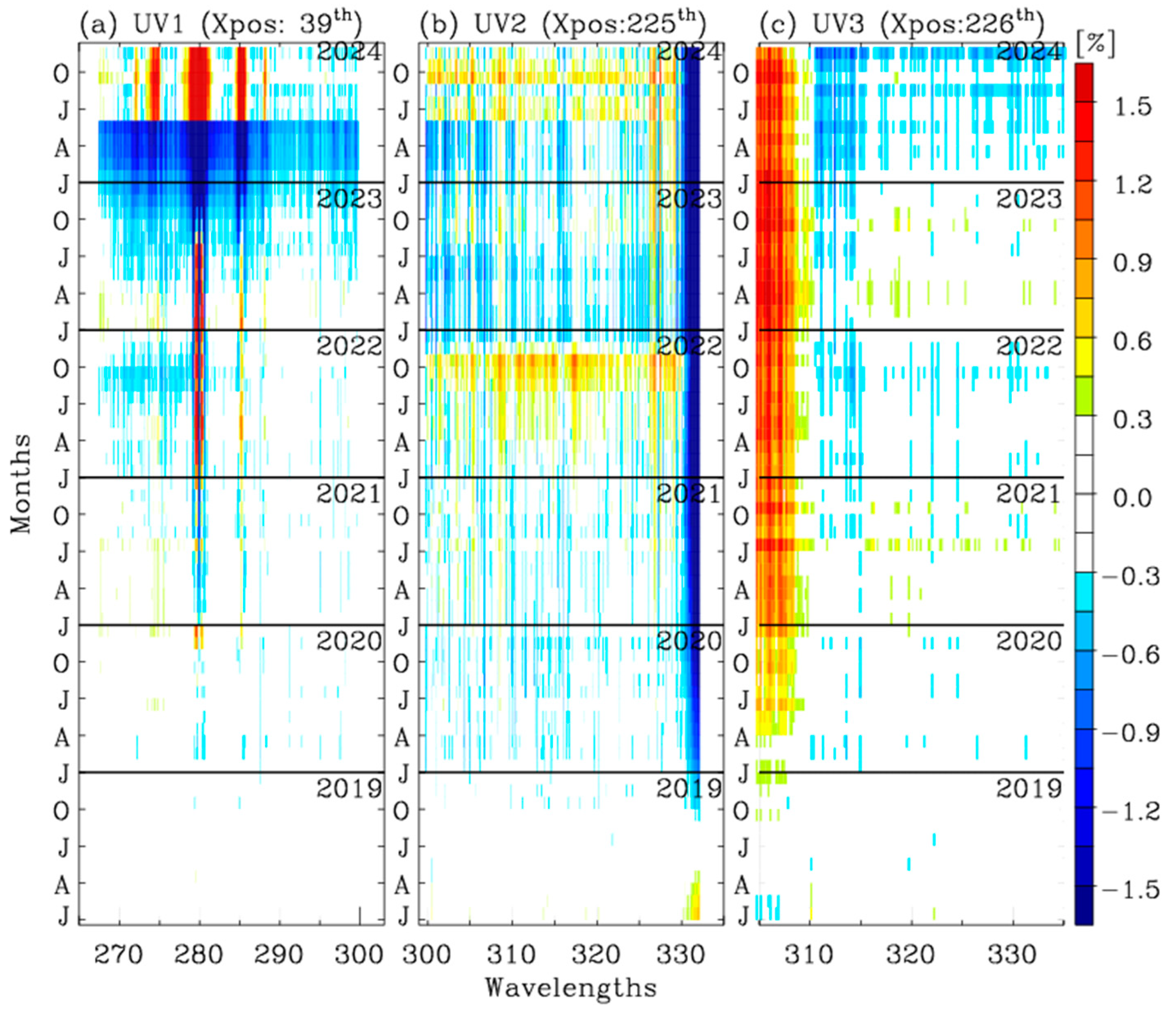
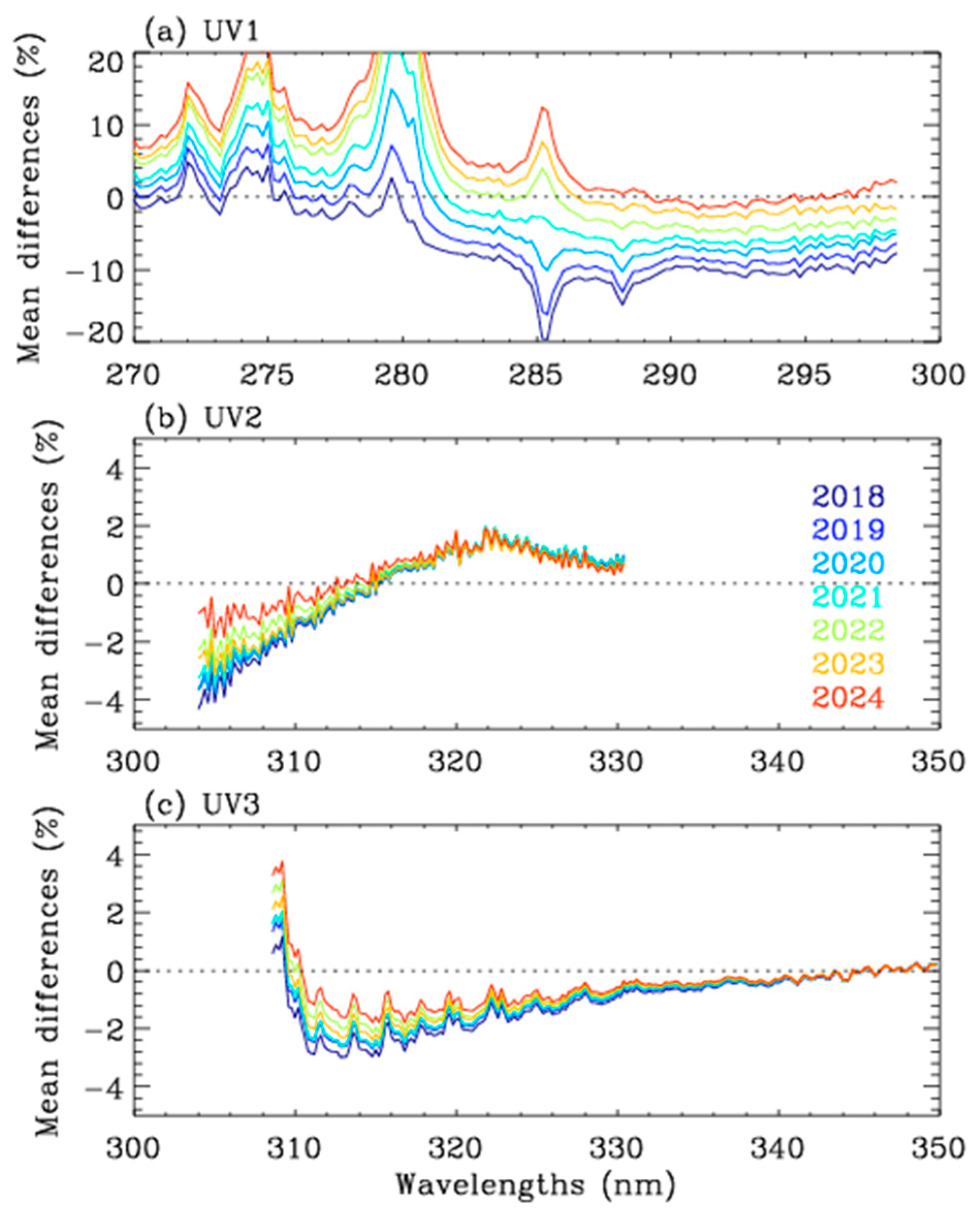
3.2.2. Irradiance Calibrations

The L1B irradiance products provide daily averaged solar irradiance measurements as a function of the CCD dimensions in normalized units to a Sun-Earth distance of 1 AU. To mitigate short-term noise, we followed the SAO2024 approach by using monthly averages of these daily irradiance spectra. Long-term changes in the irradiance measurements could indicate optical degradation, while seasonal changes may be attributed to the angular dependence of radiometric uncertainties as well as the temperature fluctuations of the optical bench. Figure 2 illustrates the temporal changes in the six years of monthly mean irradiance relative to the 2019 average for each UV band. In the UV1 band, the Mg⁺ lines (279.6 and 280.4 nm) and the Mg line (285.2 nm), which are linked to solar activity, showed a progressively increasing intensity. Aside from this trend, the UV1 irradiances remained stable within ±0.5%, except for an unusual 10% decrease in late 2023 and early 2024—an alteration that exceeds the solar activity-induced enhancement. By comparison, the UV2 and UV3 bands demonstrated strong radiometric stability throughout the mission. The UV2 irradiances varied by ±0.8% over the past six years, with the exception of the long-wavelength edges (>330 nm). The UV3 irradiance decreased within 0.3–0.5%, except at the short wavelength edges (<310 nm).

The on-orbit Instrument Spectral Response Functions (ISRFs) are parameterized as a super-Gaussian S = exp [$-{\left|{\displaystyle \frac{∆\mathsf{\lambda }}{\mathrm{w}}}\right|}^{\mathrm{k}}$], where w and k determine the width and shape of S, respectively. The slit parameters are iteratively estimated by fitting the measured solar spectrum to a high-resolution solar reference spectrum (I_o) convolved with the slit function. To improve the fitting accuracy, additional parameters―scaling factor (A), wavelength shift ($∆\mathsf{\lambda }$), scaling polynomial term (${\mathrm{P}}_{\mathrm{s}}^m$), and baseline polynomial term (${\mathrm{P}}_{\mathrm{b}}^m)$―are fitted along with the slit parameters. The simulated solar spectrum is expressed as

$${\mathit{I}}_{\mathrm{s}}\left(\lambda \right)=A\times {\mathit{I}}_o\left(\mathsf{\lambda }+\Delta \mathsf{\lambda }\right)\otimes \mathrm{S}\times {\mathrm{P}}_{\mathrm{s}}^m\left(\mathsf{\lambda }\right)+{\mathrm{P}}_{\mathrm{b}}^m\left(\mathsf{\lambda }\right)$$

(3)

where $\otimes$ denotes the convolution of the spectrum with the ISRF, and m represents the order of polynomials (3 in this study). Figure 3 evaluates the wavelength shifts ($∆\mathsf{\lambda }$) that are fitted during the derivation of the slit functions for each UV band. Here, the wavelength ranges used are 270–300 nm for UV1, 305–330 nm for UV2, and 310–335 nm for UV3, excluding the edges of irradiances due to their poor radiometric stability (see Figure 2). Since the UV1 and UV2 bands are measured using identical optics, their wavelength stability is expected to be similar. As shown in Figure 3a, the wavelength registration of the UV1 and UV2 bands is fitted to within 1.0 × 10⁻³ nm, showing no significant dependence on cross-track pixels. The adjacent pixel-to-pixel variations are smoother in the UV1 band, benefiting from the binning of the cross-track pixels. In the UV3 band, the irradiance wavelength needs to be fitted by −0.01 nm over the western cross-track pixels and by −0.018 nm over the eastern pixels. Figure 3b shows the seasonal drifts in the wavelength registration observed from all three bands, likely due to the temperature fluctuations of the optical bench. This figure also indicates that the wavelength registration gradually drifts by 0.0022 nm in UV3 over the 6.5-year span, while the UV1/UV2 band demonstrates remarkable long-term stability.

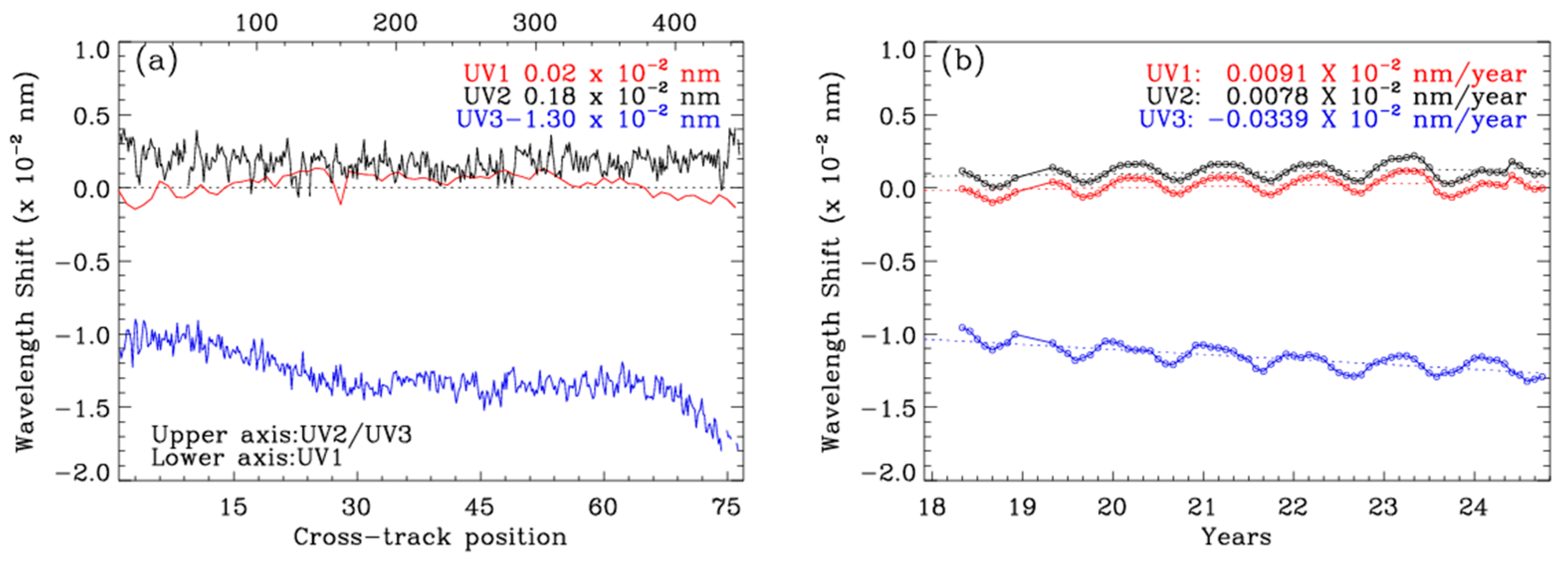
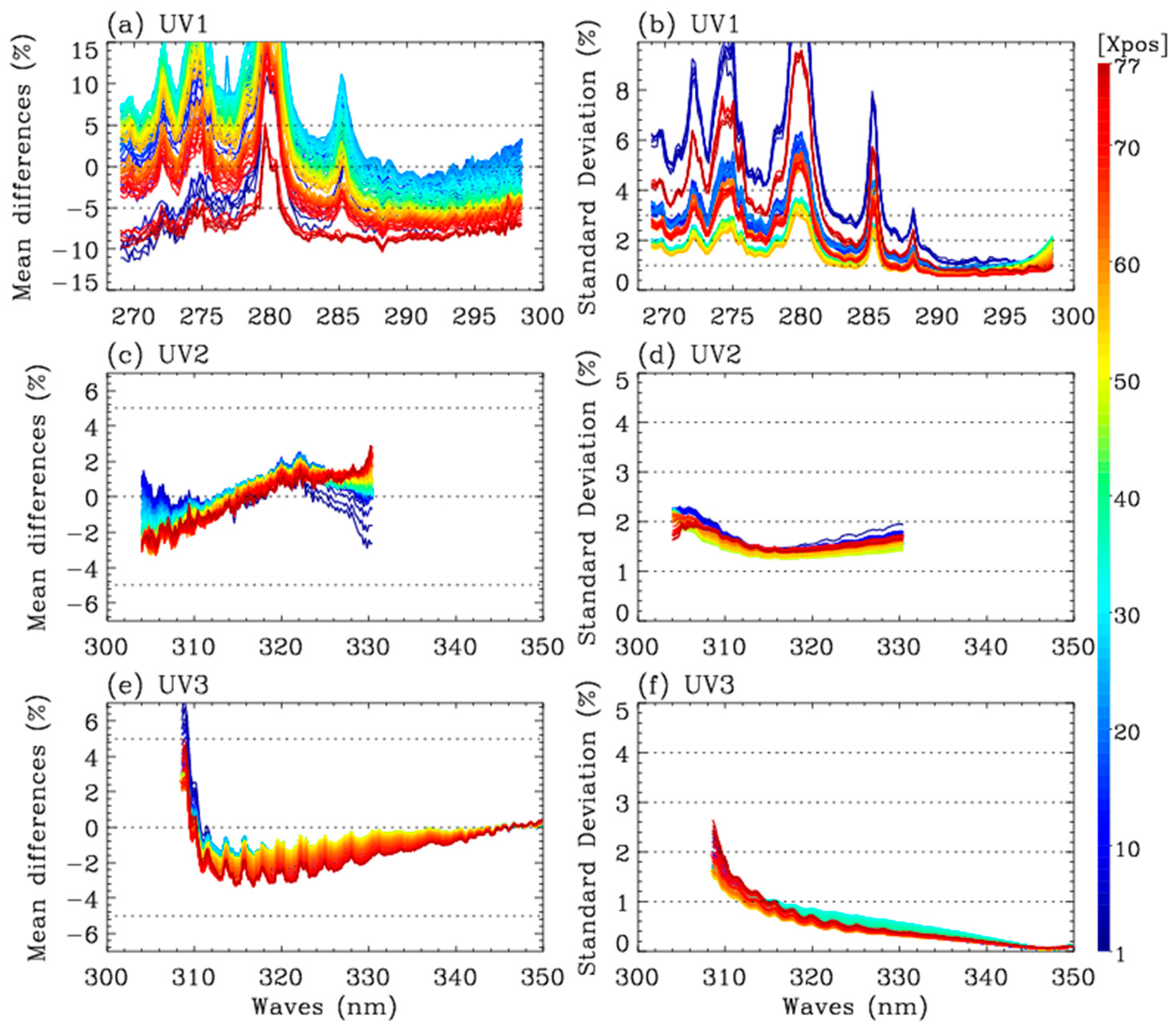
3.2.3. Radiance Calibrations

Soft calibration is an empirical method used to identify and correct radiometric biases in normalized radiance (reflectance) using forward model simulations as a baseline. The correction spectra can provide useful insights into the radiometric calibration stability for optimizing the recalibration process. As mentioned in Section 3.2.1, the TROPOMI measurements were spatially binned before performing the ozone profile retrievals for easy comparison and computational efficiency. Consequently, both UV2 and UV3 spectra were spatially binned at 77 cross-track pixels as UV1. The stability of the soft spectrum depends primarily on the ozone profile input used in the forward model calculation. To mitigate the impact of forward model input errors, we examine a tropical summer region where stratospheric ozone exhibits relatively small longitudinal variations within only a few Dobson units. According to the SAO2024 approach, the Microwave Limb Sounder (MLS) ozone profiles [35] are zonally averaged by latitude in 10° bins above 215 hPa and combined with the climatological profiles from McPeters and Labow (2012) [36]. The profile shape is subsequently adjusted to align with the zonal mean of the OMI total ozone column. Normalized radiance residuals are then calculated for three days, from 14 July to 16 July each year, in order to derive soft calibration spectra as a function of the detector arrays (wavelength and cross-track position). Figure 4 shows the derived soft spectra for each band alongside the corresponding random components of the spectral residuals. In the UV1 band, the mean residuals fluctuate significantly over the wavelengths, with pronounced offsets across cross-track positions. Even excluding the notable spikes below 285 nm, the residuals still exceed ±5%. Compared to the UV1 band, the longer UV bands exhibit less fluctuation in systematic residuals with wavelengths and cross-track pixels. The UV2 residuals range from −2% to 2%. The standard deviations of residual spectra are similar to those observed in the longer wavelengths of UV1 above 285 nm (1–2%). In the UV3 band, the normalized radiances are likely to be biased by up to −3% at 315 nm. The standard deviations remain relatively small (<1.5%).

Figure 5 shows the temporal change in the soft spectra from 2018 to 2024, which is important for addressing long-term drifts in the normalized radiances. The UV1 soft spectrum reveals a temporal drift in the radiometric errors, ranging from −10% above 290 nm to 10% below 280 nm. However, the long-term changes are less pronounced for the UV2 and UV3 normalized radiances.

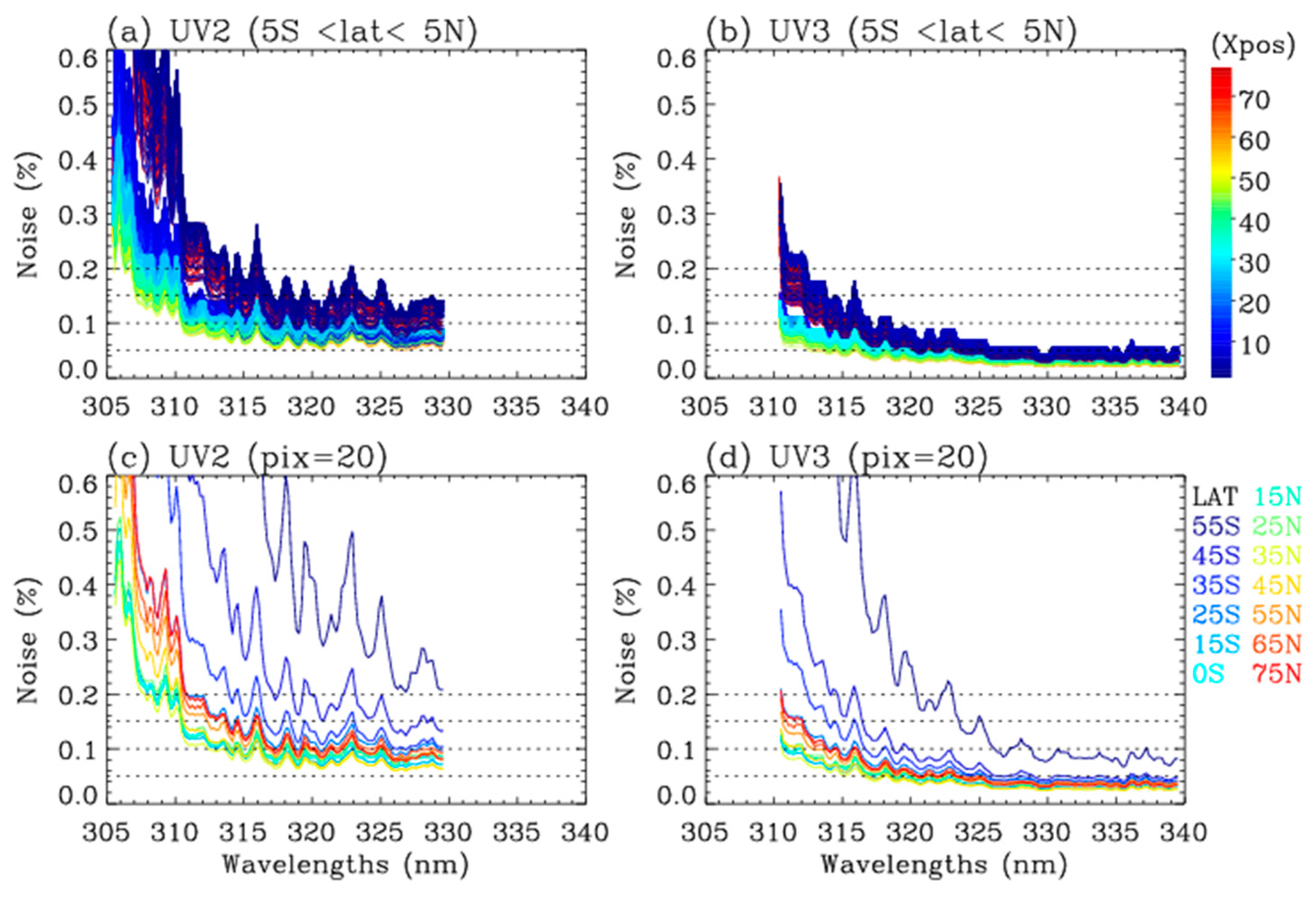
3.2.4. Measurement Error

According to Rodgers’ optimal estimation theory, measurement noise and a priori uncertainty play a crucial role in determining the weighting between a priori information and measurement data to achieve a well-behaved inversion. The L1B products provide error estimates for radiance and irradiance, each consisting of shot noise and read-out noise. When averaging a set of repeated measurements, the signal-to-noise ratio (SNR) ideally improves by a factor of √N. Accordingly, the radiance error is scaled by the square root of the number of along-track pixels, and the monthly irradiance error is scaled by the square root of the number of days before combining them as a root mean square for a normalized radiance error. Figure 6 presents the combined noise (%) from one measurement orbit. As shown, the noise level remains relatively constant at approximately 0.05% for UV3, whereas for UV2, it ranges from 0.05–0.15% for wavelengths longer than 315 nm. At shorter wavelengths, it exceeds 0.3% for UV3 and 1% for UV2. The noise is generally smaller for nadir pixels than for off-nadir pixels at lower latitudes, whereas it is enhanced at higher latitudes (larger solar zenith angles). When using a measurement constraint based on error estimates from the L1B product, many inverse processes fail either by exceeding the maximum iteration limit of 10 (‘divergence’) or by retrieving negative values in the ozone profiles (‘overfitting’). As a result, only 65% of UV2 and 36% of UV3 achieve valid convergence. To improve measurement constraints, a set of floor noise values (0.01%, 0.15%, and 0.2%) was tested, and the resulting tropospheric ozone retrievals are presented in Figure 7. It is evident that increasing the minimum noise level enhances the number of valid convergences. The valid retrieval rate rises to 97.4% when a floor noise level of 0.15% is applied to the UV3 band fitting. However, excessively loose constraints can reduce the information content in the inverse process, making it more dependent on a priori information. Considering the balance between stability and information content, the floor noise level is determined as 0.2% for UV2 and 0.1–0.15% for UV3 (0.1% for solar zenith angle < 45°).

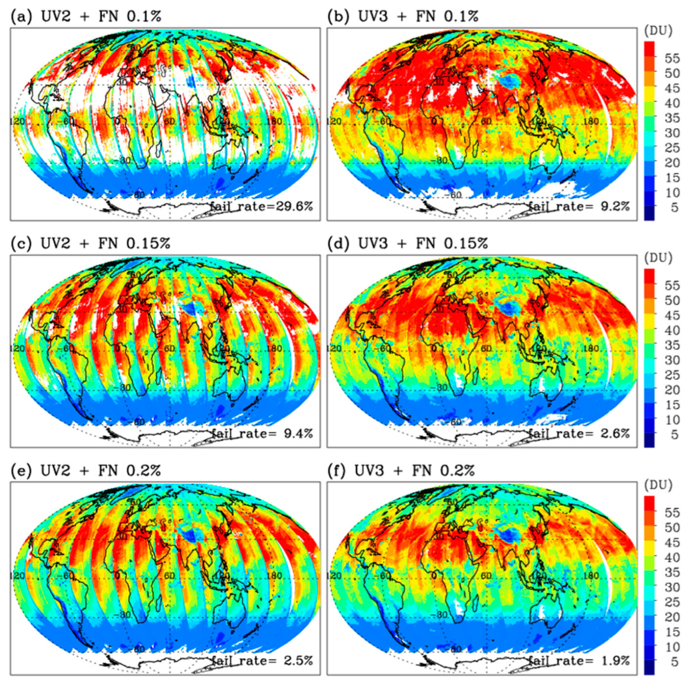
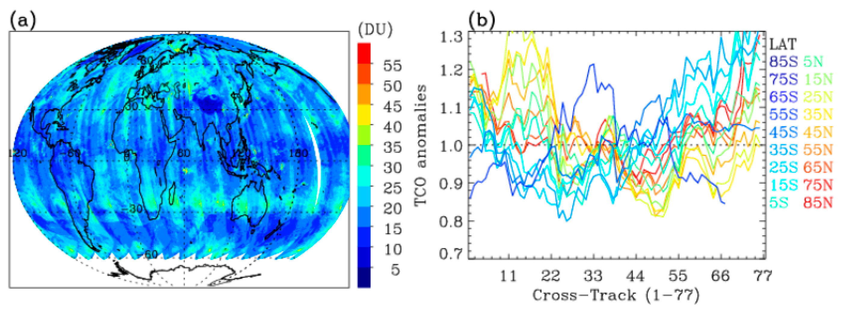
4. Comparison of Retrieval Characteristics from UV2 and UV3

Spectral range and resolution are essential for determining information content. The standard S5P product provides ozone profiles by exploiting the merged 270–330 nm spectra from the UV1 and UV2 bands. However, the UV1 band is excluded from our retrieval experiments because of dynamic radiometric uncertainties along both temporal and cross-track dimensions. Therefore, we evaluate two sets of ozone profile retrievals from the UV2 band (305–330 nm) with a 0.2% noise floor and the UV3 band (310–335 nm) with a 0.1–0.15% noise floor, respectively.

Figure 8a,b demonstrate the improved consistency of tropospheric ozone distributions between the UV2- and UV3-based retrievals by addressing radiometric biases through soft calibrations. Both retrieval outcomes depict several features, including a wave−1 structure in the tropics (with minimum values in the Pacific dominated by the Pacific Walker Circulation), elevated ozone over much of the Atlantic Ocean south of the Equator (transported by easterlies from adjacent land areas), and enhanced ozone in the northern mid-latitudes due to ozone pollution and stratospheric contributions. However, along-track stripes persist in UV2 tropospheric ozone retrievals, likely due to uncorrected radiometric uncertainties or overcorrection from soft calibration. The remaining along-track stripes were further examined by treating them as anomalies relative to the mean column across central positions. The UV2 anomalies reach approximately +10% at the 55th pixel and −20% at the rightmost pixels (Figure 8c), whereas UV3 stripes fluctuate within ±0.2–0.3%, except in the northern high-latitude bands (Figure 8d). Figure 9 presents the TROPOMI standard product, projected similarly to Figure 8, revealing substantial underestimation and pronounced along-track stripes in tropospheric ozone retrievals.

The degrees of freedom for the signal (DFS) represent the independent pieces of information available from the measurements corresponding to the trace elements of the averaging kernel matrix. A high DFS indicates that the retrieval derives most of its information from measurements, whereas a low DFS implies heavy dependence on a priori information. Here, the DFS profiles were averaged by latitude in 1° bins (Figure 10a,b) and integrated for the whole atmosphere, troposphere, and stratosphere (Figure 10c,d). The DFS profiles shows peaks in the free troposphere and just above the tropopause, with no spectral information available for retrieval above ~35 km. The integrated amount of DFS is 1.5–3 in the whole atmosphere, with 0–1.2 in the troposphere. At lower latitudes, the tropospheric UV3 retrievals contain 0.1–0.3 more DFS than the tropospheric UV2 retrievals due to the lower noise level and additional spectral information above 330 nm. On the other hand, the UV2 retrieval contains 0.1–0.3 more DFS in the stratospheric ozone due to the additional spectral information of the UV2 band below 310 nm. Note that the average DFS in the troposphere is similar (~0.5) between our research and standard products, reflecting a balance between the a priori and measurement error constraints. The measurement error constraint in our algorithm is looser (0.1–0.2%) than in the standard algorithm (0.66%/SNR = 150), but the tropospheric state is more tightly constrained by the a priori state, with climatological error values of 10–40% in our algorithm compared to a fixed 50% in the standard algorithm. Additionally, the stratospheric DFS is much higher in the standard product, benefiting from sufficient spectral information extending up to 270 nm, yielding 5–6 DFS for the full profile.

In Figure 10e,f, the fitting residuals are evaluated by normalizing them to the simulated and noise spectra, respectively. The mean measurement errors are plotted in black to assist with interpretation. The former represents the relative mean of the fitting residuals, which is required to fall within 0.3% to ensure successful retrieval. The latter corresponds to the ratio of the fitting residuals to the measurement errors (RMSs), which ideally equals 1. If the RMS deviates significantly, being either too low or too high, it suggests that the retrieval is underconstrained or overconstrained, respectively. Generally, the UV2 retrieval achieves fitting accuracies of 0.1–0.4% but exceeds 1% at latitudes higher than 45°S, where the solar zenith angles are larger than 65°. The RMS lies between 0.5 and 1.0 for most UV2 retrievals but is lower than 0.5 at high latitudes because of strong measurement constraints (noise is 0.5% or larger). The UV3 retrievals achieve better fitting accuracy, ranging from 0.1% (most cases) to 0.6% (latitudes > 30°S). Similarly, the RMS increases from 0.5–1 (most cases) to 1.5 (high latitudes).

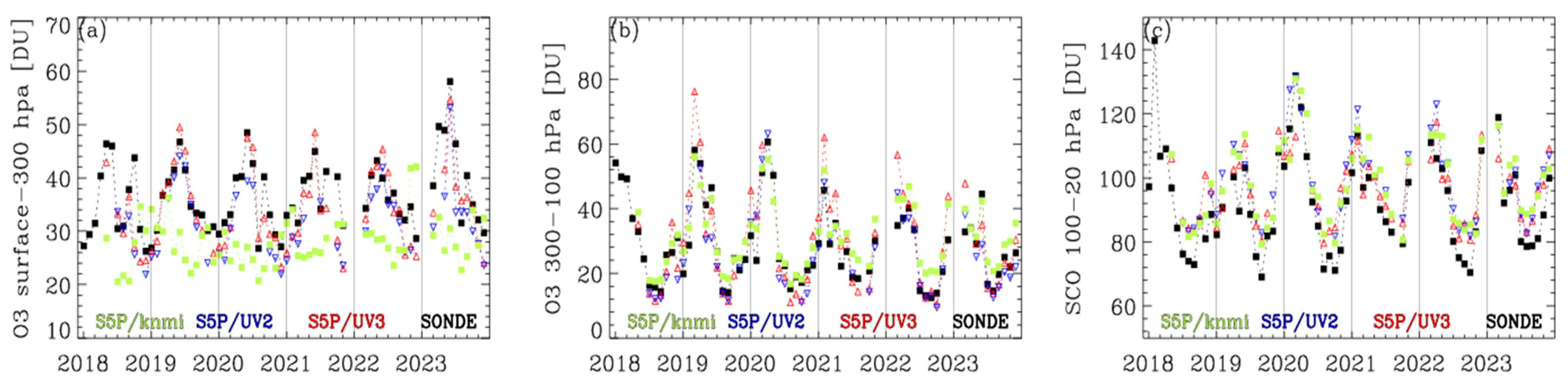
5. Comparison with Ozonesonde Measurements

We performed cross-validation on our research products (UV2 and UV3) and the TROPOMI/S5P standard products through quantitative and qualitative comparisons against independent ozonesonde observations. The two algorithms differ in their implementation details for setting up state components, radiative transfer model calculations, radiometric calibration treatments, a priori data, and a priori and measurement error covariance metrics. Consequently, notable differences are observed in their validation results, as detailed below. Figure 11 evaluates how the TROPOMI retrievals represent the daily vertical structures of ozone observed by ozonesondes in 2023 at four stations arranged by latitude from 7.6°S to 52.2°N. For comparison, high-resolution ozonesonde profiles were vertically binned at 2.5 km intervals to align with the thickness of the retrieval grids and filter out outliers or spurious values, and the TROPOMI ozone was converted into mPa to match the unit used in ozonesonde data reporting. This comparison qualitatively presents a similar conclusion for the retrieved UV2 and UV3 ozone profiles. Therefore, the UV3 retrievals were evaluated in comparison to the standard product. The UV3 ozone profiles clearly capture the enhancement of tropospheric ozone in September and October at the station of Ascension Island, located 7.6° south of the Equator in the South Atlantic Ocean, influenced by the burning of African biomass and atmospheric subsidence in Walker circulation [37,38]. Moreover, both ozonesonde soundings and UV3 retrievals consistently capture the spring maximum at King’s Park and the summer maximum in June and July at Pohang, driven by increased photochemical production before the onset of the monsoon season. However, the S5P standard profiles reflect no temporal variation in the troposphere. In contrast, the S5P standard profiles accurately represent the vertical structures of ozone in the upper troposphere and lower stratosphere (UTLS). At lower latitudes, ozone levels in the upper troposphere (10–18 km) remain relatively constant throughout the year (see Ascension Island and King’s Park). At higher latitudes, ozone-rich stratospheric air intrudes downward into the troposphere, reaching altitudes as low as 10 km (see Pohang and Lindenberg). The UTLS ozone shows noticeable seasonality owing to the minimum intrusion in fall and maximum intrusion in spring. These seasonal and latitudinal variations are reflected in the UV3 ozone profiles.

The ozone profiles paired at the Pohang station were divided into sub-columns, representing tropospheric column ozone (TCO, surface to 300 hPa), UTLS column ozone (300–100 hPa), and stratospheric column ozone (SCO, 100–30 hPa), and were averaged monthly for each year between 2018 and 2023. As shown in Figure 12, the UV2 and UV3 retrievals capture an abnormally elevated summer TCO column amount in 2023, as well as the interannual variability of the late summer ozone minimum in August, which is associated with summer monsoon activity [39]. In the UTLS region, ozone abundance was lower in summer and fall, with minimal interannual variation, whereas the maximum ozone levels in spring decreased over the last six years, captured well by our UV2/3 and standard products. The stratospheric column ozone above 100 hPa shows the seasonal cycle, which is similar to that of the UTLS ozone but with independent interannual variations, which are also effectively captured by our UV2/3 and standard products.

We quantitatively evaluated the TROPOMI ozone retrievals against the ozonesonde measurements from Pohang, Tsukuba, and King’s Park in East Asia, where ozonesondes were routinely launched weekly without major interruptions during the validation period from 2018 to 2023. The comparison metric consists of mean biases and 1$\sigma$ standard deviations and correlation coefficients for each year. In Figure 13a, the comparison of tropospheric ozone indicates a poor correlation between the standard product and ozonesondes, along with a high bias of 5–10 DU and a substantial dispersion of approximately 10 DU (−15 ± 25%). However, our research products demonstrate significant improvements in comparison statistics, with biases and dispersion reduced by a factor of two. The correlation coefficient is 0.74 for UV2 and 0.77 for UV3. The annual comparisons indicate no temporal drift. As shown in Figure 13b, the stratospheric ozone columns agree well with the ozonesonde measurements for both our research product and the standard product. A high correlation coefficient of 0.95 on average is achieved. The satellite stratospheric ozone is 3–5 DU (4%) higher than ozonesonde measurements, with a dispersion of ~5% or slightly larger.

6. Conclusions

In this study, TROPOMI UV bands 1 (267–300 nm), 2 (300–332 nm), and 3 (305–400 nm) are evaluated to identify necessary calibrations and ensure reliable retrieval quality. We conclude that recalibrating the UV1 band is challenging due to dynamic radiometric uncertainties. Therefore, we aimed to achieve consistent ozone retrievals from the UV2 and UV3 bands through the recalibration process. To reduce short-term noise, the daily irradiance measurements are averaged monthly for each CCD dimension. To match the wavelength calibration of the monthly irradiances to the reference spectrum, we found that the UV2 band requires a shift of 0.001 nm. The UV3 band requires a shift 10 times larger, ranging from −0.01 nm at the first cross-track pixel to −0.015 nm at the last pixel with a degradation trend of −0.034 × 10⁻² nm/year. In addition, temporal consistency was assessed with respect to the radiometric scale of irradiance using the 2019 mean spectrum as a baseline. In general, irradiance maintains radiometric stability within 1.0% in the UV2 band and 0.5% in the UV3 band over the past 6 years. To recalibrate irradiance and radiance simultaneously, we derived the recalibration correction spectrum for normalized radiances by analyzing the systematic components of the spectral residuals between tropical summer clear-sky measurements and their simulations. This analysis reveals that the UV2- and UV3-normalized radiances experienced a slow degradation of less than 1% during the mission.

Considering the trade-off between information content and convergence stability, the random noise errors, likely underestimated in the L1B processor, were adjusted to obtain minimum values of 0.2% for UV2 (305–330 nm) and 0.1–0.15% for UV3 (310–335 nm). As a result, the iterative OE inversion is significantly stabilized as the convergence rate rises to 97.5%. The integrated DFS is 1–1.5 in the troposphere and 3–3.5 in the entire atmosphere, with vertical sensitivity extending up to 35 km. We demonstrate the enhancement of tropospheric ozone retrievals by mitigating striping errors in UV2 and addressing offsets in UV3. However, the UV2 retrieval shows residual stripes with a bias of −2% at the rightmost nadir off-pixels, and the UV3 retrieval is highly biased at high latitudes. A better fitting accuracy is achieved for the UV3 retrieval (0.1–0.6%). Our retrievals effectively capture the enhancement of tropospheric ozone driven by biomass burning, anthropogenic emissions, and the hemispheric transport of stratospheric ozone observed through ozonesonde soundings. In particular, we demonstrate the capability of our retrievals to represent interannual variations in tropospheric and stratospheric ozone throughout the full S5P mission. For tropospheric ozone, the mean bias is −2.5 DU for UV2 and −0.43 DU for UV3, with a similar dispersion slightly exceeding 5 DU and correlation coefficients ranging from 0.74 to 0.77. For stratospheric ozone, the mean bias is 8.1 ± 11.52 DU (R = 0.96) for UV2 and 5.7 ± 10.49 DU (R = 0.96) for UV3.

In conclusion, the SAO2024 algorithm, originally developed for OMI, was successfully implemented to retrieve TROPOMI ozone profiles. The results demonstrate its capability to consistently retrieve ozone profiles with recalibrated normalized radiances from UV2 and UV3. The next step in this project is to compare the OMI and TROPOMI ozone profiles and address the discrepancies between them, with the goal of developing reliable, merged products suitable for long-term trend analysis.

References

1. Lefohn, A.S.; Malley, C.S.; Smith, L.; Wells, B.; Hazucha, M.; Simon, H.; Naik, V.; Mills, G.; Schultz, M.G.; Paoletti, E.; et al. Tropospheric ozone assessment report: Global ozone metrics for climate change, human health, and crop/ecosystem research. Elem. Sci. Anthr. 2018, 6, 27. [Google Scholar] [CrossRef]
2. Mills, G.; Pleijel, H.; Malley, C.S.; Sinha, B.; Cooper, O.R.; Schultz, M.G.; Neufeld, H.S.; Simpson, D.; Sharps, K.; Feng, Z.; et al. Tropospheric Ozone Assessment Report: Present-day tropospheric ozone distribution and trends relevant to vegetation. Elem. Sci. Anthr. 2018, 6, 47. [Google Scholar] [CrossRef]
3. Monks, P.S.; Archibald, A.T.; Colette, A.; Cooper, O.; Coyle, M.; Derwent, R.; Fowler, D.; Granier, C.; Law, K.S.; Mills, G.E.; et al. Tropospheric ozone and its precursors from the urban to the global scale from air quality to short-lived climate forcer. Atmos. Chem. Phys. 2015, 15, 8889–8973. [Google Scholar] [CrossRef]
4. Bourgeois, I.; Peischl, J.; Neuman, J.A.; Brown, S.S.; Thompson, C.R.; Aikin, K.C.; Allen, H.M.; Angot, H.; Apel, E.C.; Baublitz, C.B.; et al. Large contribution of biomass burning emissions to ozone throughout the global remote troposphere. Proc. Natl. Acad. Sci. USA 2021, 118, e2109628118. [Google Scholar] [CrossRef] [PubMed]
5. Miller, A.J. A review of satellite, observations of atmospheric ozone. Planet. Space Sci. 1989, 37, 1539–1554. [Google Scholar] [CrossRef]
6. Bhartia, P.K.; Heath, D.F.; Fleig, A.F. Observation of anomalously small ozone densities in south polar stratosphere during October 1983 and 1984. In Proceedings of the Symposium on Dynamics and Remote Sensing of the Middle Atmosphere, 5th Scientific Assembly, International Association of Geomagnetism and Aeronomy, Prague, Czech Republic, 5–17 August 1985. [Google Scholar]
7. Burrows, J.P.; Weber, M.; Buchwitz, M.; Rozanov, V.; Ladstätter-Weißenmayer, A.; Richter, A.; DeBeek, R.; Hoogen, R.; Bramstedt, K.; Eichmann, K.-U.; et al. The Global Ozone Monitoring Experiment (GOME): Mission Concept and First Scientific Results. J. Atmos. Sci. 1999, 56, 151–175. [Google Scholar] [CrossRef]
8. van der A, R.J.; Van Oss, R.F.; Piters, A.J.M.; Fortuin, J.P.F.; Meijer, Y.J.; Kelder, H.M. Ozone profile retrieval from recalibrated Global Ozone Monitoring Experiment data. J. Geophys. Res. 2002, 107, 4239. [Google Scholar] [CrossRef]
9. Hoogen, R.; Rozanov, V.V.; Burrows, J.P. Ozone profiles from GOME satellite data: Algorithm description and first validation. J. Geophys. Res. Atmos. 1999, 104, 8263–8280. [Google Scholar] [CrossRef]
10. Liu, X.; Chance, K.; Sioris, C.E.; Spurr, R.J.D.; Kurosu, T.P.; Martin, R.V.; Newchurch, M.J. Ozone profile and tropospheric ozone retrievals from the Global Ozone Monitoring Experiment: Algorithm description and validation. J. Geophys. Res. 2005, 110, D20307. [Google Scholar] [CrossRef]
11. Liu, X.; Chance, K.; Sioris, C.E.; Kurosu, T.P. Impact of using different ozone cross sections on ozone profile retrievals from Global Ozone Monitoring Experiment (GOME) ultraviolet measurements. Atmos. Chem. Phys. 2007, 7, 3571–3578. [Google Scholar] [CrossRef]
12. Munro, R.; Siddans, R.; Reburn, W.J.; Kerridge, B.J. Direct measurement of tropospheric ozone distributions from space. Nature 1998, 392, 168–171. [Google Scholar] [CrossRef]
13. Levelt, P.F.; Joiner, J.; Tamminen, J.; Veefkind, J.P.; Bhartia, P.K.; Stein Zweers, D.C.; Duncan, B.N.; Streets, D.G.; Eskes, H.; van der A, R.; et al. The Ozone Monitoring Instrument: Overview of 14 years in space. Atmos. Chem. Phys. 2018, 18, 5699–5745. [Google Scholar] [CrossRef]
14. Flynn, L.; Long, C.; Wu, X.; Evans, R.; Beck, C.T.; Petropavlovskikh, I.; McConville, G.; Yu, W.; Zhang, Z.; Niu, J.; et al. Performance of the Ozone Mapping and Profiler Suite (OMPS) products. J. Geophys. Res. Atmos. 2014, 119, 6181–6195. [Google Scholar] [CrossRef]
15. Pan, C.; Yan, B.; Flynn, L.; Beck, T.; Chen, J.; Huang, J. Recent Improvements to NOAA-20 Ozone Mapper Profiler Suite Nadir Profiler Sensor Data Records. In Proceedings of the 2021 IEEE International Geoscience and Remote Sensing Symposium (IGARSS), Brussels, Belgium, 11–16 July 2021; pp. 7924–7926. [Google Scholar]
16. Veefkind, J.P.; Aben, I.; McMullan, K.; Förster, H.; de Vries, J.; Otter, G.; Claas, J.; Eskes, H.J.; de Haan, J.F.; Kleipool, Q.; et al. TROPOMI on the ESA Sentinel-5 Precursor: A GMES mission for global observations of the atmospheric composition for climate, air quality and ozone layer applications. Remote Sens. Environ. 2012, 120, 70–83. [Google Scholar] [CrossRef]
17. De Smedt, I.; Pinardi, G.; Vigouroux, C.; Compernolle, S.; Bais, A.; Benavent, N.; Boersma, F.; Chan, K.-L.; Donner, S.; Eichmann, K.-U.; et al. Comparative assessment of TROPOMI and OMI formaldehyde observations and validation against MAX-DOAS network column measurements. Atmos. Chem. Phys. 2021, 21, 12561–12593. [Google Scholar] [CrossRef]
18. Torres, O.; Jethva, H.; Ahn, C.; Jaross, G.; Loyola, D.G. TROPOMI aerosol products: Evaluation and observations of synoptic-scale carbonaceous aerosol plumes during 2018–2020. Atmos. Meas. Tech. 2020, 13, 6789–6806. [Google Scholar] [CrossRef]
19. Keppens, A.; Di Pede, S.; Hubert, D.; Lambert, J.-C.; Veefkind, P.; Sneep, M.; De Haan, J.; ter Linden, M.; Leblanc, T.; Compernolle, S.; et al. 5 years of Sentinel-5P TROPOMI operational ozone profiling and geophysical validation using ozonesonde and lidar ground-based networks. Atmos. Meas. Tech. 2024, 17, 3969–3993. [Google Scholar] [CrossRef]
20. An, Y.; Wang, X.; Ye, H.; Shi, H.; Wu, S.; Li, C.; Sun, E. Ozone Profile Retrieval Algorithm Based on GEOS-Chem Model in the Middle and Upper Atmosphere. Remote Sens. 2024, 16, 1335. [Google Scholar] [CrossRef]
21. Mettig, N.; Weber, M.; Rozanov, A.; Arosio, C.; Burrows, J.P.; Veefkind, P.; Thompson, A.M.; Querel, R.; Leblanc, T.; Godin-Beekmann, S.; et al. Ozone profile retrieval from nadir TROPOMI measurements in the UV range. Atmos. Meas. Tech. 2021, 14, 6057–6082. [Google Scholar] [CrossRef]
22. Zhao, F.; Liu, C.; Cai, Z.; Liu, X.; Bak, J.; Kim, J.; Hu, Q.; Xia, C.; Zhang, C.; Sun, Y.; et al. Ozone profile retrievals from TROPOMI: Implication for the variation of tropospheric ozone during the outbreak of COVID-19 in China. Sci. Total Environ. 2021, 764, 142886. [Google Scholar] [CrossRef] [PubMed]
23. Rodgers, C.D. Inverse Methods for Atmospheric Sounding; World Scientific: Singapore, 2000. [Google Scholar]
24. Tikhonov, A.N. Solution of Incorrectly Formulated Problems and the Regularization Method. Sov. Math. Dokl. 1963, 4, 1035–1038. [Google Scholar]
25. Bak, J.; Liu, X.; Yang, K.; Gonzalez Abad, G.; O’Sullivan, E.; Chance, K.; Kim, C.-H. An improved OMI ozone profile research product version 2.0 with collection 4 L1b data and algorithm updates. Atmos. Meas. Tech. 2024, 17, 1891–1911. [Google Scholar] [CrossRef]
26. Liu, X.; Bhartia, P.K.; Chance, K.; Spurr, R.J.D.; Kurosu, T.P. Ozone profile retrievals from the Ozone Monitoring Instrument. Atmos. Chem. Phys. 2010, 10, 2521–2537. [Google Scholar] [CrossRef]
27. Kroon, M.; de Haan, J.F.; Veefkind, J.P.; Froidevaux, L.; Wang, R.; Kivi, R.; Hakkarainen, J.J. Validation of operational ozone profiles from the Ozone Monitoring Instrument. J. Geophys. Res. Atmos. 2011, 116, D18305. [Google Scholar] [CrossRef]
28. Ludewig, A.; Kleipool, Q.; Bartstra, R.; Landzaat, R.; Leloux, J.; Loots, E.; Meijering, P.; van der Plas, E.; Rozemeijer, N.; Vonk, F.; et al. In-flight calibration results of the TROPOMI payload on board the Sentinel-5 Precursor satellite. Atmos. Meas. Tech. 2020, 13, 3561–3580. [Google Scholar] [CrossRef]
29. de Haan, J.F.; Wang, P.; Sneep, M.; Veefkind, J.P.; Stammes, P. Introduction of the DISAMAR radiative transfer model: Determining instrument specifications and analysing methods for atmospheric retrieval (version 4.1.5). Geosci. Model Dev. 2022, 15, 7031–7050. [Google Scholar] [CrossRef]
30. Labow, G.J.; Ziemke, J.R.; McPeters, R.D.; Haffner, D.P.; Bhartia, P.K. A total ozone-dependent ozone profile climatology based on ozonesondes and Aura MLS data. J. Geophys. Res. Atmos. 2015, 120, 2537–2545. [Google Scholar] [CrossRef]
31. Veefkind, P.; Keppens, A.; de Haan, J. TROPOMI ATBD Ozone Profile v1.0.0. Available online: https://sentinel.esa.int/documents/247904/2476257/Sentinel-5P-TROPOMI-ATBD-Ozone-Profile.pdf (accessed on 12 December 2024).
32. Bak, J.; Liu, X.; Wei, J.C.; Pan, L.L.; Chance, K.; Kim, J.H. Improvement of omi ozone profile retrievals in the upper troposphere and lower stratosphere by the use of a tropopause-based ozone profile climatology. Atmos. Meas. Tech. 2013, 6, 2239–2254. [Google Scholar] [CrossRef]
33. Bak, J.; Liu, X.; Spurr, R.; Yang, K.; Nowlan, C.R.; Miller, C.C.; Abad, G.G.; Chance, K. Radiative transfer acceleration based on the principal component analysis and lookup table of corrections: Optimization and application to UV ozone profile retrievals. Atmos. Meas. Tech. 2021, 14, 2659–2672. [Google Scholar] [CrossRef]
34. Loyola, D.G.; Gimeno García, S.; Lutz, R.; Argyrouli, A.; Romahn, F.; Spurr, R.J.D.; Pedergnana, M.; Doicu, A.; Molina García, V.; Schüssler, O. The operational cloud retrieval algorithms from TROPOMI on board Sentinel-5 Precursor. Atmos. Meas. Tech. 2018, 11, 409–427. [Google Scholar] [CrossRef]
35. Livesey, N.J.; Read, W.G.; Wagner, P.A.; Froidevaux, L.; Santee, M.L.; Schwartz, M.J.; Lambert, A.; Millan Valle, L.F.; Pumphrey, H.C.; Manney, G.L.; et al. EOS MLS Version 5.0x Level 2 and 3 Data Quality and Description Document, Tech. Rep., Jet Propulsion Laboratory D-105336 Rev. B, 30 January 2022. Available online: https://mls.jpl.nasa.gov/eos-aura-mls/documentation.php (accessed on 31 January 2025).
36. McPeters, R.D.; Labow, G.J. Climatology 2011: An MLS and sonde derived ozone climatology for satellite retrieval algorithms. J. Geophys. Res. Atmos. 2012, 117, D10303. [Google Scholar] [CrossRef]
37. Jensen, A.A.; Thompson, A.M.; Schmidlin, F.J. Classification of Ascension Island and Natal ozonesondes using self-organizing maps. J. Geophys. Res. Atmos. 2012, 117, D04302. [Google Scholar] [CrossRef]
38. Thompson, A.M.; Witte, J.C.; Smit, H.G.J.; Oltmans, S.J.; Johnson, B.J.; Kirchhoff, V.W.J.H.; Schmidlin, F.J. Southern Hemisphere Additional Ozonesondes (SHADOZ) 1998–2004 tropical ozone climatology: 3. Instrumentation, station-to-station variability, and evaluation with simulated flight profiles. J. Geophys. Res. Atmos. 2007, 112, D03304. [Google Scholar] [CrossRef]
39. Bak, J.; Song, E.-J.; Lee, H.-J.; Liu, X.; Koo, J.-H.; Kim, J.; Jeon, W.; Kim, J.-H.; Kim, C.-H. Temporal variability of tropospheric ozone and ozone profiles in the Korean Peninsula during the East Asian summer monsoon: Insights from multiple measurements and reanalysis datasets. Atmos. Chem. Phys. 2022, 22, 14177–14187. [Google Scholar] [CrossRef]
Figure 1. Geolocation boundaries of UV1 (black) at the first cross-track pixel (binned over four pixels) across five scanlines (2501–2505) and the corresponding UV2 (red) and UV3 (blue) pixels.
Remotesensing 17 00779 g001
Figure 2. Temporal changes in monthly mean irradiances as a function of wavelength during the period of 2019 to 2024: (a) UV1, (b) UV2, and (c) UV3. At the nadir cross-track position, the irradiances are averaged over each month and subtracted from the baseline, which is the mean irradiance in 2019. All 497 wavelengths are evaluated for UV1 and UV2, while only the first 200 wavelengths are evaluated for UV3, focusing on the ozone fitting window. J, A, J, and O on the Y-axis represent January, April, July, and October, respectively.
Remotesensing 17 00779 g002
Figure 3. (a) Pixel-to-pixel variations of wavelength shift (nm) in the monthly solar irradiances of July 2023. The legend refers to the different channels, with the mean value over all the cross-track positions. (b) Temporal variations of wavelength shift (nm) at the middle cross-track positions. The legend presents the trend value of the shift per year.
Remotesensing 17 00779 g003
Figure 4. (a,c,e) TROPOMI soft spectrum, derived as the average differences between measured and simulated normalized radiances for UV1, UV2, and UV3, respectively. (b,d,f) Corresponding standard deviations. Different color coding represents the cross-track position (Xpos). The calculation was performed using tropical clear-sky measurements from three days: 13–15 July 2022 (latitude: <±20°, cloud fraction: <0.2, and solar zenith angle: <60°). An input ozone profile is prepared by merging the zonal mean of daily MLS v5.0 stratospheric ozone profiles above 215 hPa and a climatological tropospheric ozone profile.
Remotesensing 17 00779 g004
Figure 5. TROPOMI soft spectrum from 2018 to 2024 for (a) UV1, (b) UV2, and (c) UV3 only at the 37th cross-track pixel in the 77 binned arrays.
Remotesensing 17 00779 g005
Figure 6. Root mean squares of individual radiance and irradiance random noise errors (%) for orbit #29377 on 15 June 2023 for (a,c) UV2 and (b,d) UV3. The radiance error is scaled by the square root of co-added, along-track pixels, and the monthly irradiance error is scaled by the square root of the number of days before combining them. Upper panels: different colors represent individual cross-track noise spectra in the tropics. Lower panels: noise spectra for the 35th cross-track pixel averaged over 10° latitude bands.
Remotesensing 17 00779 g006
Figure 7. Daily maps of the tropospheric ozone columns (surface to 400 hPa) on 15 June 15 2023 from (a,c,e) UV2 and (b,d,f) UV3 retrieval experiments, respectively. Note that soft calibration is not applied in this comparison. Data screening was performed to ensure that iterations terminated within 10 cycles and that all retrieved ozone values were positive, with the legend indicating the rate of invalid retrievals.
Remotesensing 17 00779 g007
Figure 8. (a,b) Daily maps of tropospheric ozone columns below 400 hPa, with soft calibrations applied to the UV2 and UV3 bands, respectively. The corresponding comparison without applying soft calibration is shown in Figure 7e (UV2) and Figure 7d (UV3). (c,d) Cross-track pixel-dependent tropospheric column ozone (TCO) anomalies quantified as the ratio of each cross-track column to the mean column across central positions 11–67.
Remotesensing 17 00779 g008
Figure 9. Same as Figure 8, but for the TROPOMI standard product. (a) tropospheric ozone columns (TCO). (b) Cross-track pixel-dependent TCO anomalies.
Remotesensing 17 00779 g009
Figure 10. Degrees of freedom for signal (DFS), averaged in 1° latitude bins for retrieved ozone profiles from (a) UV2 and (b) UV3, as shown in Figure 8. The red line indicates the tropopause level. (c,d) Total, stratospheric, and tropospheric DFS. (e,f) Mean relative residuals (%) and root mean square of residuals (scaled by the measurement errors) with measurement errors (%). For visualization alignment, noise values were increased tenfold.
Remotesensing 17 00779 g010
Figure 11. Comparison of ozone profiles. (a,d,g,j) The 2023 ozone profiles (in mPa) measured by ozonesonde at Ascension Island (14.2°W, 7.6°S), King’s Park (114.2°E, 22.3°N), Pohang (129.4°E, 36.0°N), and Lindenberg (14.1°E, 52.2°N). (b,e,h,k) S5P ozone profile retrievals from UV3. (c,f,i,l) S5P/KNMI standard ozone profiles.
Remotesensing 17 00779 g011
Figure 12. Six-year time series of monthly averaged sub-column ozone at the Pohang station at different atmospheric layers: (a) surface to 300 hPa (TCO), (b) 300 to 100 hPa (UTLS), and (c) 100 hPa to 30 hPa (SCO). The black line represents the ozonesonde time series, along with the S5P standard (green), UV2 retrieval (blue), and UV3 retrieval (red).
Remotesensing 17 00779 g012
Figure 13. Statistical comparison of TROPOMI research products (UV2 and UV3) and standard products with ozonesonde data from Pohang, Tsukuba, and King’s Park for (a) tropospheric ozone columns below 300 hPa and (b) stratospheric column ozone above 300 hPa during 2018–2023. The mean bias (star symbols), 1-σ standard deviation (error bars), and correlation coefficient (square symbols) are virtually presented for each year, with overall statistics summarized in the legend.
Remotesensing 17 00779 g013