Abstract
Spaceborne inverse synthetic aperture ladar (ISAL) can achieve high-resolution imaging of satellite targets. However, because the amplitudes of satellite microvibration are comparable to the ladar wavelength, the echoes will contain both space-variant and space-invariant phase errors. These errors will lead to azimuthal image defocus and impede target analysis and identification. In this paper, we establish a phase error estimation model based on satellite vibration characteristics. Based on this model, we propose a vibration phase error compensation algorithm using prior information and adaptive windowing. Compared to conventional algorithms, this algorithm utilizes prior information to improve estimation accuracy while significantly reducing computational complexity. Furthermore, high-accuracy phase function estimation can be achieved through maximum likelihood estimation and adaptive window filtering, thereby enabling the compensation of vibration phase errors. Both simulation and real imaging experiments validate the effectiveness and robustness of the proposed algorithm.
1. Introduction
Inverse synthetic aperture ladar (ISAL) represents a breakthrough in super-resolution imaging by overcoming the diffraction limit. Compared to conventional microwave radar, ISAL achieves superior spatial resolution in reduced acquisition time by leveraging the shorter wavelengths of the optical band. Additionally, through laser heterodyne detection, ISAL enables high-fidelity imaging of ultralong-distance targets [1,2]. When deployed on orbital platforms, ISAL can circumvent the decoherence effects in optical heterodyne detection signals caused by atmospheric turbulence, thereby facilitating target classification and identification [3,4]. Consequently, spaceborne ISAL presents significant potential for the detection and identification of space targets, particularly satellites.
However, the short laser wavelength presents both advantages and challenges. The ISAL operates at wavelengths on the order of micrometers, which is comparable to the microvibration amplitude of satellite targets. This high sensitivity to satellite vibration introduces significant phase errors in the echo signals, causing image defocus and severely degrading the ISAL imaging quality. Consequently, compensation for vibration-induced phase errors is essential for achieving high-resolution imaging [5].
Satellite target microvibration consists of two components: translational vibration and angular vibration. Translational vibration occurs along the line-of-sight direction relative to the ladar. This motion generates space-invariant phase errors, which remain constant in both azimuthal and range dimensions. Angular vibration refers to the vibration of the target as it rotates relative to the ladar. It produces space-variant phase errors that vary with the target’s azimuthal dimension. In satellite ISAL imaging, angular vibration is the dominant motion component [6,7]. Therefore, the resulting space-variant phase errors cannot be ignored.
Multiple strategies have been developed to address ISAL/SAL vibration phase error compensation. Established methods include the phase gradient autofocus (PGA) [8], maximum contrast algorithm [9], and minimum entropy algorithm [10]. PGA, the most widely adopted method, demonstrates robust performance by estimating strong scattering points across range cells without assuming any specific phase error form. Recent advances have introduced novel compensation techniques. Hu et al. [11] developed a multichannel interferometric processing method for ISAL vibration phase estimation. Their approach models phase errors using polynomials and extracts phase error differentials through multichannel interference. Yin et al. [12] proposed a delay-based conjugate multiplication method that suppresses pairwise echoes during ISAL platform amplitude variations. However, these methods are limited to compensating space-invariant phase errors, leaving space-variant phase errors unaddressed.
To address this issue, Song et al. [13] developed an autofocusing method based on nonparametric estimation of two distinctive points for space-variant phase error compensation. However, this method’s reliance on isolated distinctive points in the target scene restricts its practical applications. Subsequently, Song et al. [14] introduced the phase gradient matrix autofocusing (PGMA) algorithm. This method employs weighted least squares linear fitting (WLSLF) to iteratively estimate vibration phase errors, enabling compensation of higher-order space-variant phase errors from satellite vibration. However, PGMA’s performance is limited by two factors: the inclusion of misestimated range cells reduces both estimation accuracy and computational efficiency, and the requirement for manual parameter input leads to unstable compensation results. Wang et al. [7] proposed a frequency descent minimum entropy optimization algorithm that improves the estimation of both space-variant and space-invariant phase errors. Despite its enhanced accuracy, the algorithm’s high computational cost makes it impractical for real-time spaceborne ISAL imaging.
For these considerations, we propose an improved vibration phase error compensation algorithm based on prior information and adaptive windowing. First, we establish a phase error estimation model based on satellite vibration characteristics, transforming the vibration phase error estimation into a phase function estimation problem. Then, range-compressed data undergo PGA preprocessing to identify viable range cells as prior information. Using this information, we extract corresponding image segments for adaptive window width estimation. These estimated widths are applied to window the main scatterers’ centers in each range cell, effectively filtering clutter interference. The phase functions are then estimated using maximum likelihood estimation. Finally, vibration phase errors are determined through weighted least-squares (WLS) estimation. Echo data compensation is performed iteratively to achieve a well-focused image. Simulation and experimental results demonstrate that our method effectively compensates both space-variant and space-invariant phase errors caused by satellite vibration, offering high accuracy, computational efficiency and robust performance.
The paper is organized as follows. In Section 2, we introduce the ISAL turntable imaging model and echo signal model with target vibration effects. Section 2.3 details the developed vibration phase error estimation model and describes the detailed implementation of the proposed algorithm. Experimental results using both simulation and real measurement data are presented in Section 3. Section 4 provides a discussion of the obtained results. Finally, the conclusion is given in Section 5.
2. Methods
2.1. Imaging Geometry
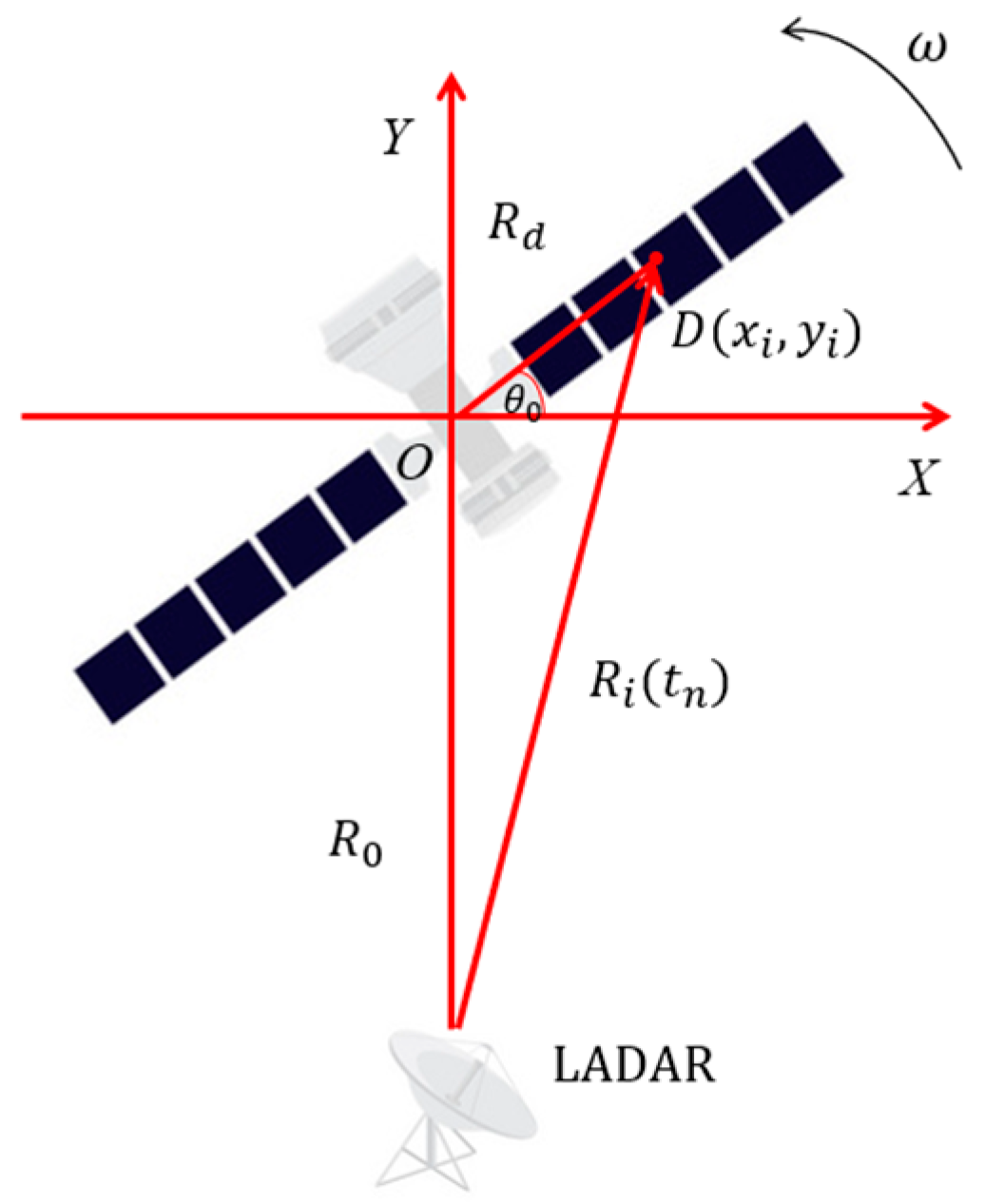
In ISAL imaging, the synthetic aperture is formed by the relative motion between the target and the ladar. The imaging geometry can be simplified by assuming a stationary ladar while decomposing satellite target motion into translational and rotational components. After range migration compensation and initial phase correction eliminate the translational motion, the imaging geometry becomes equivalent to a turntable model where the target rotates around a reference point, as illustrated in Figure 1.
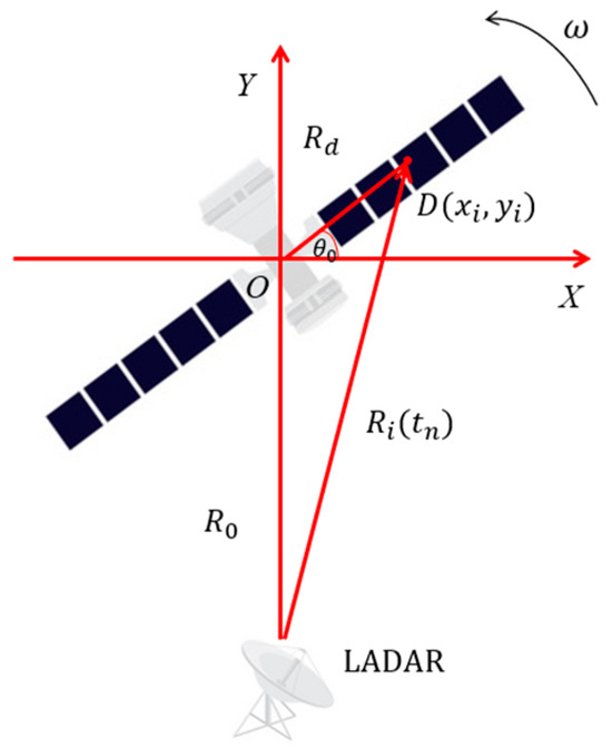
Figure 1.
ISAL imaging equivalent turntable model.
In Figure 1, the ladar is positioned in the far field. A Cartesian coordinate system is set up with the target’s equivalent rotation center O, as the origin. In this system, the Y-axis is defined by the ladar’s line of sight, while the X-axis is oriented perpendicular to it. The satellite target revolves around the origin O with an angular speed of ω, with no translational motion relative to the ladar. Point D represents the ith scattering point on the target with coordinates , and denotes the angle between OD and the X-axis. When the target is not vibrating, the distance from scattering point D to the ladar can be expressed as:
where represents the distance between the ladar and origin O, represents the distance from scattering point D to origin O, and denotes the slow time. Since the target-to-ladar distance is much greater than the target dimensions (), the equation can be approximated as:
Since the coherent accumulation angle required for ISAL imaging is very small, i.e., the value of is small, can be approximated as:
In the turntable model, satellite microvibration can be decomposed into translational vibration and angular vibration. The translational vibration corresponds to the radial displacement component of the satellite from origin O to the ladar along the Y-axis, while the angular vibration represents the angular displacement component of the satellite relative to origin O. Satellite microvibration is induced by both internal and external forces. Assuming these influences follow a smooth random process, the resulting translational and angular vibrations can be modeled as independent harmonic motions [15,16], expressed, respectively, as:
where denotes the instantaneous vibration-induced radial distance variation along the ladar line of sight direction, , and denote the amplitude, frequency, and initial phase of the p-th translational vibration component, respectively, represents the instantaneous angular displacement of the satellite relative to the origin O, , and indicate the amplitude, frequency, and initial phase of the p-th angular vibration component, respectively. Due to target vibration, the distance from ladar to scattering point D becomes:
2.2. Signal Model
ISAL systems conventionally utilize linear frequency-modulated (LFM) signals for target imaging, and its mathematical expression is:
where the rectangle function
and is the fast time, is the full time, is the pulse width, is the carrier frequency. The ratio is the chirp rate, where is the bandwidth of the transmitted LFM signal. Assuming k scattering points in the target scene, the received echo signal can be expressed as:
where and denote the backscattering coefficient and the distance between the ladar and the ith scattering point, respectively, and represents the speed of light. After the dechirping, range compression, and the residue video phase (RVP) compensation [17] of the ISAL target echo signals, we can obtain the following:
where is the reference distance corresponding to the reference channel and is the optical wavelength.
Setting and substituting (5) into (8), we can obtain:
where . The first phase term in Equation (9), induced by target rotation, encodes the azimuthal position information of the ith scattering point. The second term corresponds to space-variant phase error arising from angular vibration, which exhibits dependence on the target’s azimuthal coordinates. The third term describes the space-invariant phase error caused by translational vibration. Both the second and third terms induce azimuthal defocusing in ISAL imagery and necessitate compensation to achieve optimal focusing performance.
2.3. Proposed Vibration Phase Error Compensation Algorithm
In this section, we establish a phase error estimation model for satellite vibrations. Building on this model, we propose an iterative compensation algorithm that incorporates prior information and adaptive windowing. The algorithm utilizes prior data to select appropriate range cells for estimation, thereby reducing computational complexity while enhancing estimation accuracy. In each iteration, adaptive window center filtering is applied to improve both the efficiency and stability of the algorithm.
2.3.1. Phase Error Estimation Model
Phase error estimation typically begins with the data in the range-compressed domain. The range-compressed data matrix of the outlier echo is denoted as , where is the range cell number, is the total number of range cells, and is the sequence of pulse numbers, is the total number of pulses. During data processing, the phase function of the echo signal is sampled at the pulse repetition frequency of the slow-time sampling. Since the constant term does not impact the imaging process, it is ignored. As a result, Equation (9) can be rewritten as follows:
where denotes the Doppler frequency of the ith scattering point, normalized by the pulse repetition frequency. The azimuthal frequency position of the ith scattering point is represented by , ranging from − to , and is the pulse repetition frequency. We define the normalized angular vibration error parameter as , and the normalized translational vibration error parameter as . Assume that the Doppler frequency of the strongest scatterer in the mth range cell is , and treat the other scatterers as clutter terms. The signal for the mth range cell can then be written as:
where denotes the magnitude of the strongest scatterer in the mth range cell, and represents the clutter term in the mth range cell. For the same slow-time, the space-variant and space-invariant phase errors induced by satellite microvibration are identical across all range cells. Therefore, the phase function of the signal for all range cells can be expressed as follows:
where
is the phase function matrix, is the vibrational error parameter matrix, and is the eigenvalue matrix, consisting of the magnitude of 1 and the azimuthal frequency position of the strongest scatterer at each range cell. represents the clutter matrix.
The linear Equation (12) describes the vibration phase error estimation model, which makes no assumptions about the clutter terms, thus making it applicable to a broad range of azimuth space-variant phase error estimation problems. From Equation (11), it is evident that the slope of the phase function corresponds to the azimuthal frequency position of the prominent point, meaning the eigenvalue matrix can be derived from the phase function matrix . Therefore, through appropriate filtering, the vibration error parameter can be obtained by linearly fitting and . Consequently, the estimation of the vibration error parameter can be transformed into the estimation of the phase function .
2.3.2. Vibration Phase Error Compensation Algorithm
Through the above analysis, we need to estimate the phase function for each range cell. However, the phase function can only be accurately estimated when the range cell contains prominent points. In complex observation scenarios, not all range cells contain prominent points, and some phase functions may be inaccurately estimated due to the effects of vibration and noise. To ensure accurate estimation, it is necessary to preprocess the data to identify the range cells that can be used for fitting, serving as a priori information for the algorithm. If too few range cells are selected, the statistical regularity of the clutter background is lost, which negatively affects estimation accuracy. Conversely, selecting too many range cells introduces additional estimation errors and increases computational effort. In this paper, we use the PGA algorithm for data preprocessing. First, the PGA algorithm is used to estimate the space-invariant phase error for all range cells, which is then used to compensate for the image. The image entropy index is employed to quantify the image quality, and the expression for image entropy is as follows [18]:
where denotes the normalized image power, defined as:
Calculate the entropy values for each compensated image and the average of all entropy values, denoted as and , respectively. The range cells in with values greater than are marked as having larger estimation errors and are recorded using the vector , where indicates a correct estimation and indicates an incorrect estimation. This vector can then be used as a priori information.
After obtaining the priori information, we can further estimate the phase function and the eigenvalue matrix . The phase function can be estimated using the maximum likelihood estimation (MLE) method in the PGA algorithm, which has been shown to achieve the Cramér–Rao lower bound on the estimation variance. The expression for the maximum likelihood estimation is:
where denotes the phase error gradient function of the mth range cell, * denotes the conjugate operation, and arg [⋅] denotes the phase operation. After obtaining the phase error gradient function, the phase function can be obtained by accumulating it. The expression for the phase function is:
where denotes the phase function of the mth range cell. To improve the estimation accuracy of the phase function, we adopt a scheme that adds a window centered on the main scatterer of each range cell, which helps eliminate the interference from high-frequency noise and clutter. This approach involves critical trade-offs: excessively narrow windows truncate critical signal components, while oversized windows degrade the signal-to-noise ratio (SNR) through clutter inclusion. In this paper, we propose an adaptive window width estimation method based on curve-fitting envelope extraction. The specific steps are as follows:
Step1: Normalized amplitude.
Based on the priori information, i.e., the vector , the corresponding range cells are selected to form a new complex image. This image is then circularly shifted, with the point having the highest pixel intensity for each range cell moved to the center of the image. The energies of the points in all azimuth cells for each range direction of the image are accumulated to obtain a one-dimensional vector. The calculation formula is:
where is the two-dimensional complex image after cyclic shifting, denotes the sequence of range cells after selection, and is the total number of vectors for which .
Step2: Downsampling and curve fitting.
The one-dimensional vectors obtained are searched for two maxima, and these data points are extracted for downsampling purposes. Segmented Hermite interpolation is then performed to fit the filtered data points.
Step3: Window width estimation.
Search along the fitted curve from both edges towards the center, and detect the first points on both sides where the curve changes drastically (with a change greater than three times the previous value). The distance between these two points is calculated as the window width for the windowing, as shown in Figure 2. To ensure the convergence of the window width, the search for the window width in each iteration begins from the position of the previous window’s width.
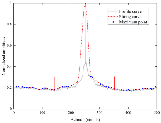
Figure 2.
Waveform contour after curve fitting.
This approach facilitates phase function matrix estimation during iterative windowing processes, operating independently of prior window width specifications. It adaptively selects the appropriate window width, thereby eliminating dependence on external parameter tuning. Furthermore, it can adapt to various ISAL images, improving the algorithm’s estimation accuracy and robustness.
After estimating the a priori phase function matrix , the slope of the phase function, according to Equation (11), represents the azimuthal frequency position of the prominent point. Therefore, the priori eigenvalue matrix can be obtained by calculating the slope of . The vibration error parameter matrix is then estimated using the weighted least squares fitting (WLS) method. Its expression is:
where is the weighted diagonal matrix computed from the variance of the phase gradient function and . The superscript T denotes the transpose operation, and var [⋅] denotes the variance of the enclosed quantity.
Based on the vibration phase error parameter matrix, we can construct the phase error compensation matrix and the discrete Fourier transform matrix [13]:
where , is the digitized azimuthal frequency. The compensation of the vibration phase error can be achieved as follows [13]:
where denotes the refocused image and the operator “” is the Hadamard product.
For satellite target ISAL imaging, the echo signal typically has a low SNR. This necessitates iterative refinement of the aforementioned processing steps to achieve optimal image focus. The convergence criterion terminates iterations when the residual phase error falls below a predetermined threshold, at which point the optimized image is generated.
2.3.3. Flowchart of the Proposed Algorithm
To improve the iterative efficiency, our priori information is computed only once. Subsequent iterations estimate only the range cells where , significantly reducing the computational load. By combining priori information with adaptive windowing, the proposed algorithm does not require user input parameters and is not dependent on isolated prominent points in the imaging scene. This allows for efficient and precise compensation of the phase errors caused by satellite microvibration, making it applicable to a wide range of scenarios. Figure 3 shows the flowchart of the proposed algorithm. Figure 3a shows the flowchart for computing a priori information, and Figure 3b illustrates the iterative compensation process of the algorithm.
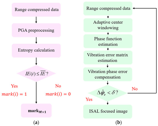
Figure 3.
Flowchart of the proposed algorithm (a) priori information; (b) iterative compensation.
3. Results
In this section, computer simulation and indoor ISAL imaging experiments are presented to demonstrate the performance of the proposed algorithm.
3.1. Simulation Result
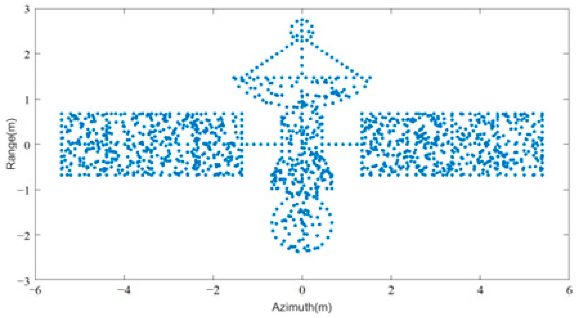
In this subsection, simulation experiments are conducted for a satellite model consisting of approximately 1500 scattering points. The backward scattering coefficients of these points are randomly distributed between 0.2 and 0.4. Gaussian white noise is added to simulate scattering speckle noise. The satellite target scattering point model is shown in Figure 4.
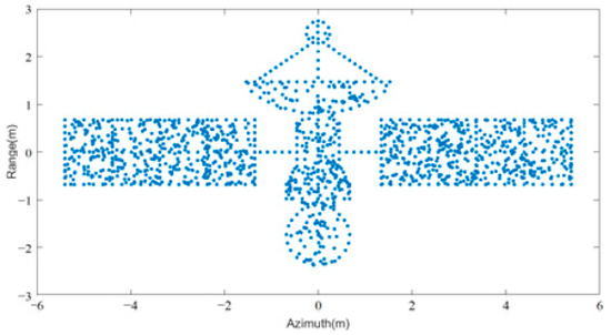
Figure 4.
Satellite scatter points model.
The satellite microvibration is modeled according to Equation (4). The parameters for the translational and angular vibrations are based on the ETS-VI, OICETS, and Micius in-orbit test data provided by the European Space Agency (ESA) and other institutions. The main vibration frequency is distributed within 200 Hz, and the maximum acceleration is controlled to be within 0.5 m/s2 through filtering and other methods [6,19,20]. The angular vibration power spectral density fitting function for the Olympus satellite, provided by ESA, is expressed as [19]:
where denotes the frequency of vibration in Hertz. Accordingly, vibration components of 180 Hz, 120 Hz and 70 Hz are added to the simulation with amplitudes calculated from (22) and set random initial phases. The parameters of the simulated experimental ladar are shown in Table 1.

Table 1.
Parameters used in the simulation.
After injecting vibration phase errors, we controlled echo SNR via calibrated noise. Signals at 5, 0, and −5 dB SNR were processed via RD, PGA, PGMA, and the proposed algorithm, followed by a systematic comparison of their imaging results. In addition, we quantified the image quality using image entropy, image contrast and peak signal-to-noise ratio (PSNR). Reduced entropy values signify enhanced focusing precision, whereas elevated contrast and PSNR values correlate with improved edge sharpness and effective noise suppression, respectively. The expression for image entropy was previously provided, and the expressions for image contrast and PSNR are as follows:
where is the averaging function, represents the maximum possible grayscale value of the image, and refers to the ideal image without noise and vibration phase errors.
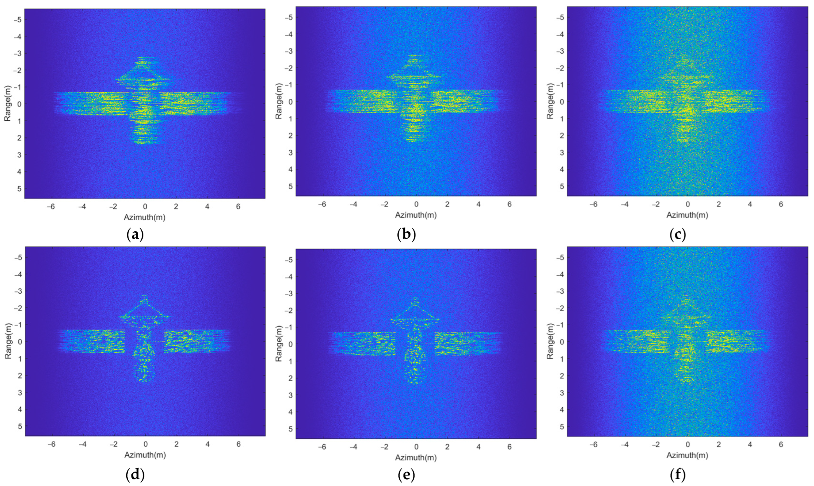
Figure 5 shows the imaging results obtained using the RD, PGA, PGMA, and the proposed algorithm for echo signals with SNRs of 5, 0, and −5 dB. To reduce side lobes, the image is processed by adding a Hamming window in the slow-time dimension. Figure 5a–c demonstrate the RD algorithm’s imaging performance across varying SNR levels. The results reveal fundamental limitations in vibration phase error compensation manifesting as azimuthal defocusing that intensifies progressively toward the scene margin. Figure 5d–f indicates partial success in the central region focusing through space-invariant phase error correction, though significant edge defocusing persists due to unresolved space-variant phase errors. Notably, decreasing SNR levels lead to progressively degraded space-invariant phase error compensation performance in PGA outputs. The PGMA algorithm shows improved focusing uniformity between central and edge regions from Figure 5g–i, yet residual defocusing persists along solar panel extremities, as evidenced in the annotated regions (Figure 5i red insets). Similar to PGA, PGMA’s performance exhibits SNR-dependent degradation in edge preservation. By contrast, the proposed algorithm demonstrates superior focusing performance at both the center and edges of the image across various SNR levels.
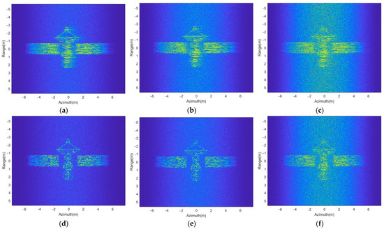

Figure 5.
Imaging results of the four algorithms at SNRs of 5, 0, and −5 dB. (a–c) RD; (d–f) PGA; (g–i) PGMA; (j–l) proposed algorithm.
Table 2 lists the image entropy, image contrast, and PSNR of the images shown in Figure 5, with the results obtained by compensating for the true values of the vibration phase errors as a reference. As shown in Table 2, the image entropy decreases progressively from the RD algorithm to the proposed algorithm. For the image contrast and PSNR metrics, both increase progressively from the RD algorithm to the proposed algorithm. Furthermore, the metrics corrected using the proposed algorithm are very close to those obtained by compensating with the true values, validating the proposed algorithm’s ability to compensate for vibration phase errors.
Table 2.
Image quality of different algorithms at different SNRs.
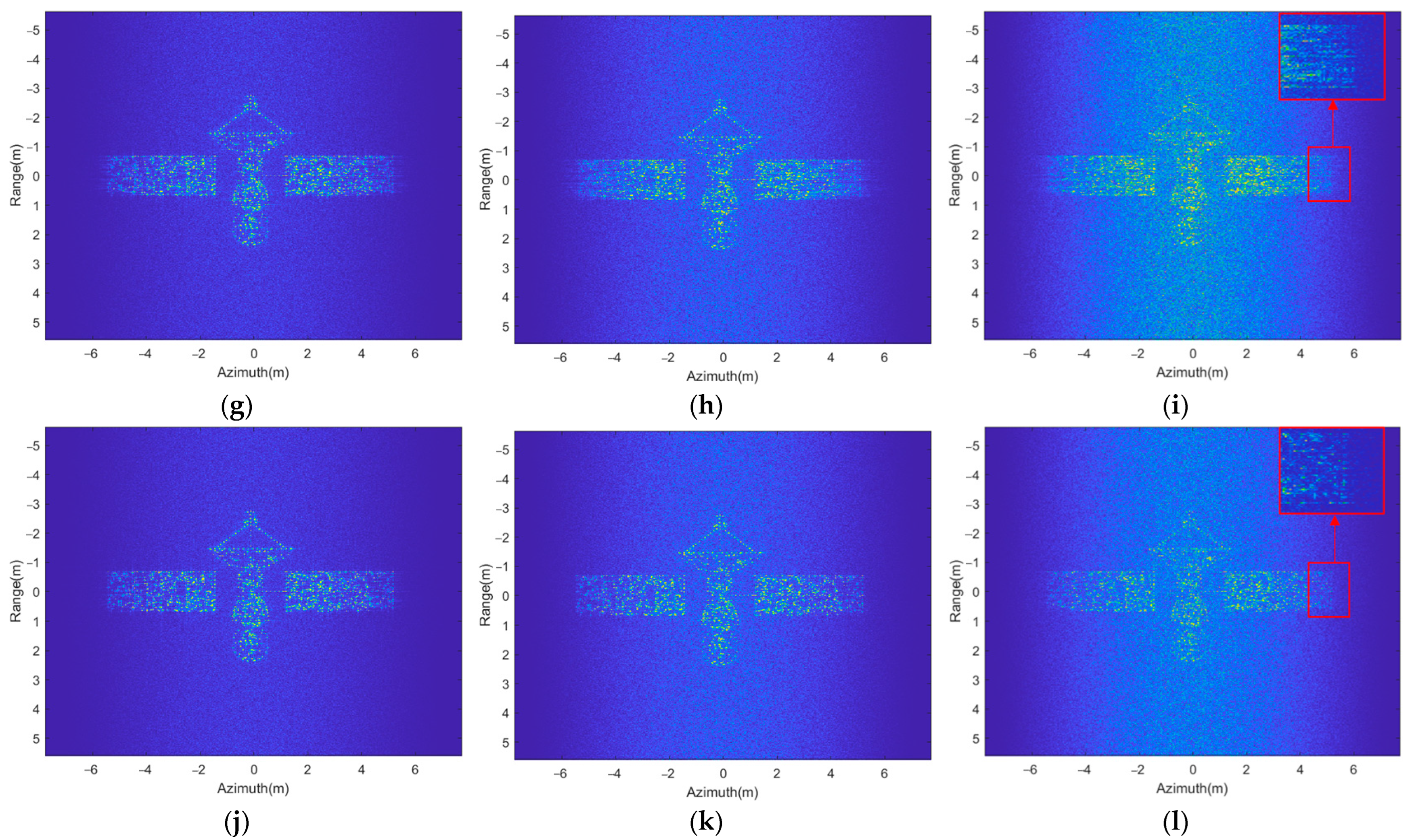
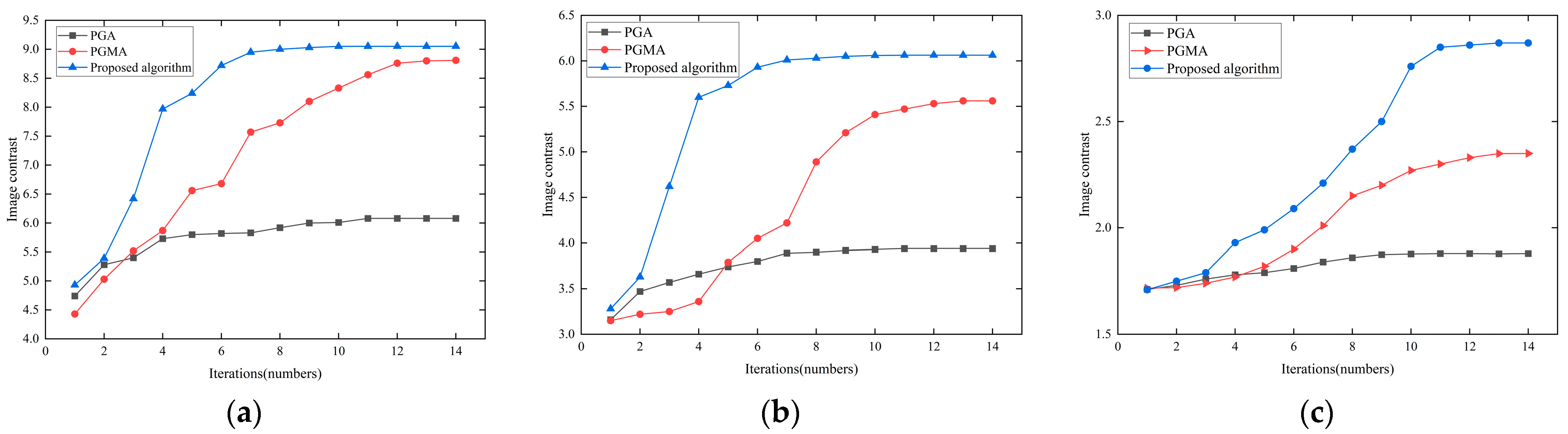
To demonstrate the iterative efficiency of the proposed algorithm, we plotted the curve of image contrast versus the number of iterations for the proposed algorithm, PGMA algorithm, and PGA algorithm at SNRs of 5 dB, 0 dB, and −5 dB, as shown in Figure 6.
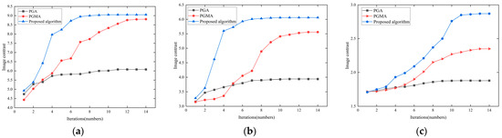
Figure 6.
Image contrast versus number of iterations curves for imaging results obtained with PGA, PGMA and the proposed algorithm at SNRs of 5, 0, and −5 dB. (a) 5 dB; (b) 0 dB; (c) −5 dB.
In Figure 6, the image contrast of all three algorithms progressively improves with increasing iterations. Comprehensive analysis reveals that the PGA algorithm achieves convergence after approximately eight iterations, yet demonstrates inferior phase compensation performance. The PGMA algorithm consistently requires 12–14 iterations to reach convergence. In comparison, the proposed algorithm attains convergence within 6–8 iterations under high SNR conditions and 10–12 iterations under low SNR conditions, representing a reduction in the number of iterations by 16% to 50%. Notably, the proposed algorithm maintains superior imaging quality throughout all iterative cycles compared to both PGA and PGMA methods, demonstrating its highest iterative efficiency.
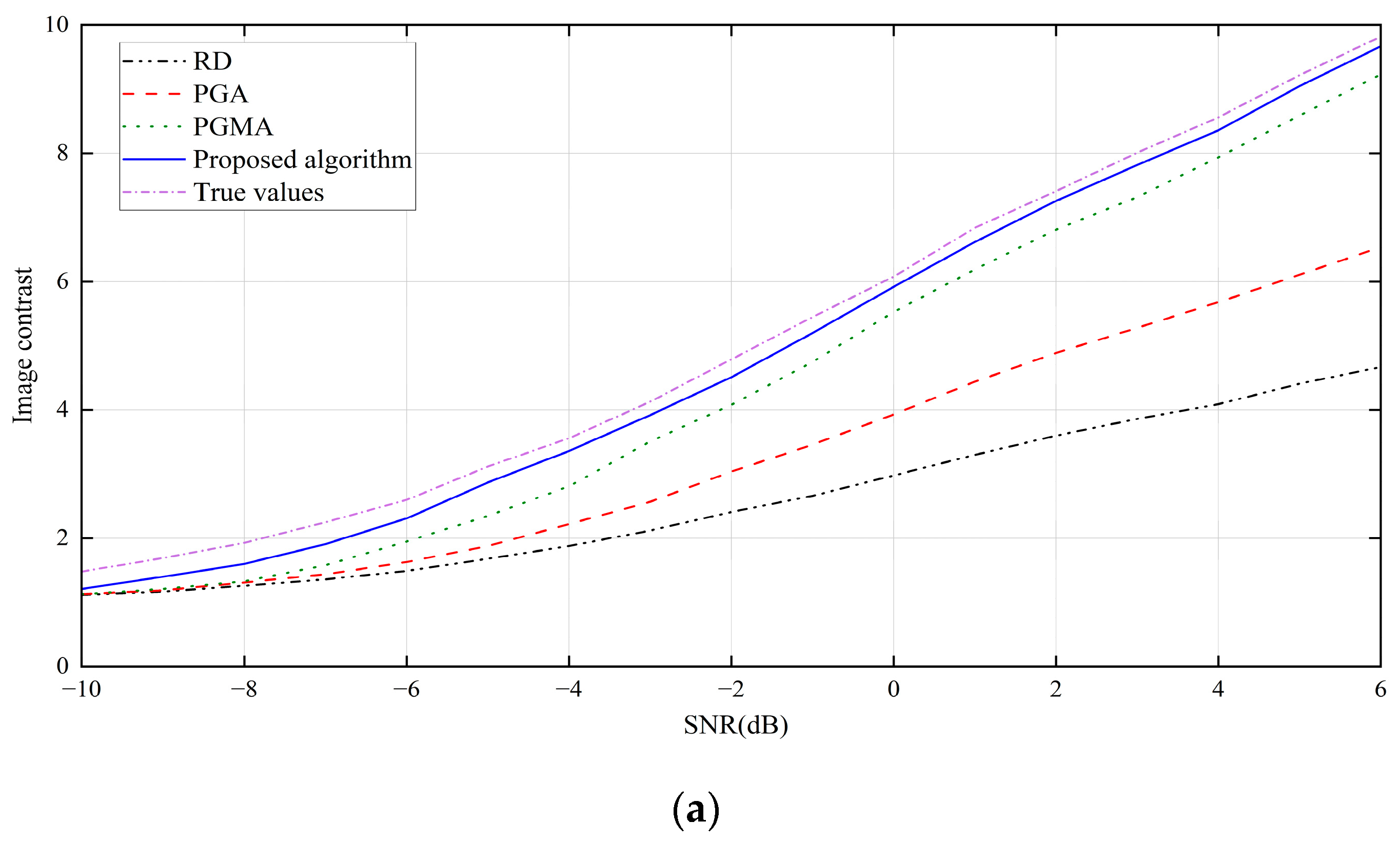
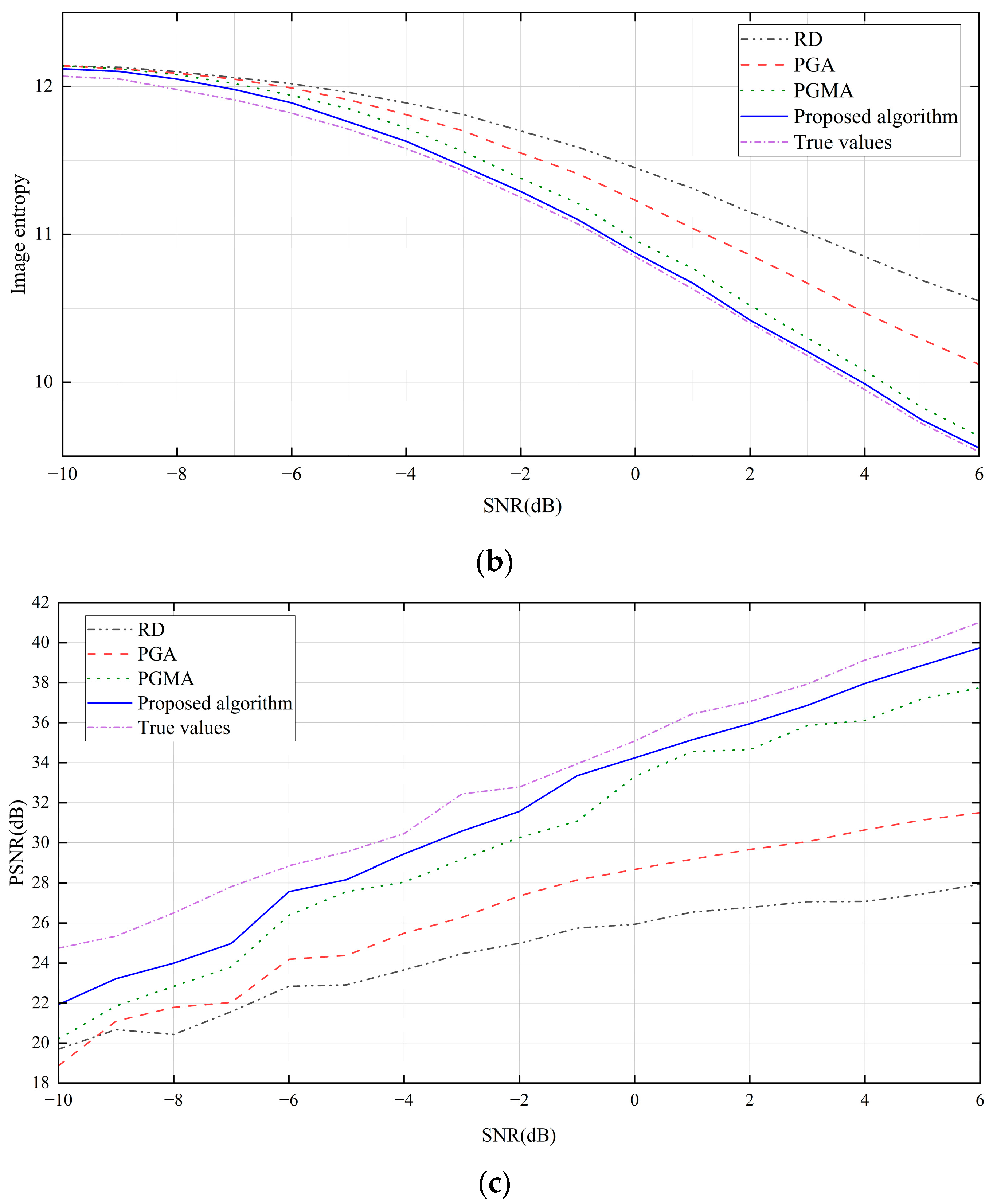
To further verify the compensation ability of the proposed algorithm under different SNR conditions, we repeated the simulation with SNR ranging from −10 dB to 6 dB. To reduce randomness, five simulations were conducted for each condition. The resulting curves of the average values for image contrast, image entropy and PSNR as a function of SNR are shown in Figure 7.
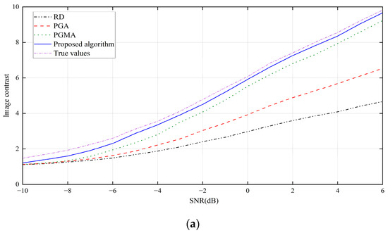
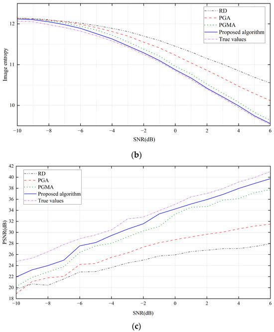
Figure 7.
Variation curve of image quality with SNRs. (a) image contrast; (b) image entropy; (c) PSNR.
In Figure 7, it can be seen that the proposed algorithm outperforms the other algorithms under all SNR conditions. The proposed algorithm significantly outperforms the PGMA algorithm at SNR greater than −7 dB. When the SNR is greater than −5 dB, the performance of the proposed algorithm is very close to that of using the true value compensation for the vibration phase error, thus validating the robustness of the proposed algorithm.
3.2. Real Data Experiment Results
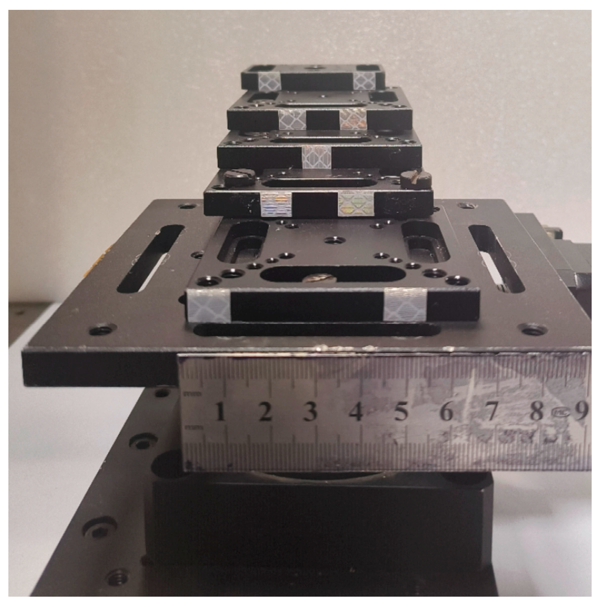
The real measurement data were obtained through indoor imaging experiments, and the main system parameters of the ladar are shown in Table 1. In these experiments, the target distance and the target rotational angular velocity were set to 3 m and 48 mrad/s, respectively. The experimental target comprised an X-configured structure featuring nine 3M retroreflective strips (1.0 × 0.7 cm each), mounted on a precision rotary stage. With physical dimensions of 5.7 cm (azimuth) × 17.0 cm (range), the target’s spatial configuration and corresponding optical reference image with scale markers are presented in Figure 8.

Figure 8.
Optical picture of targets.
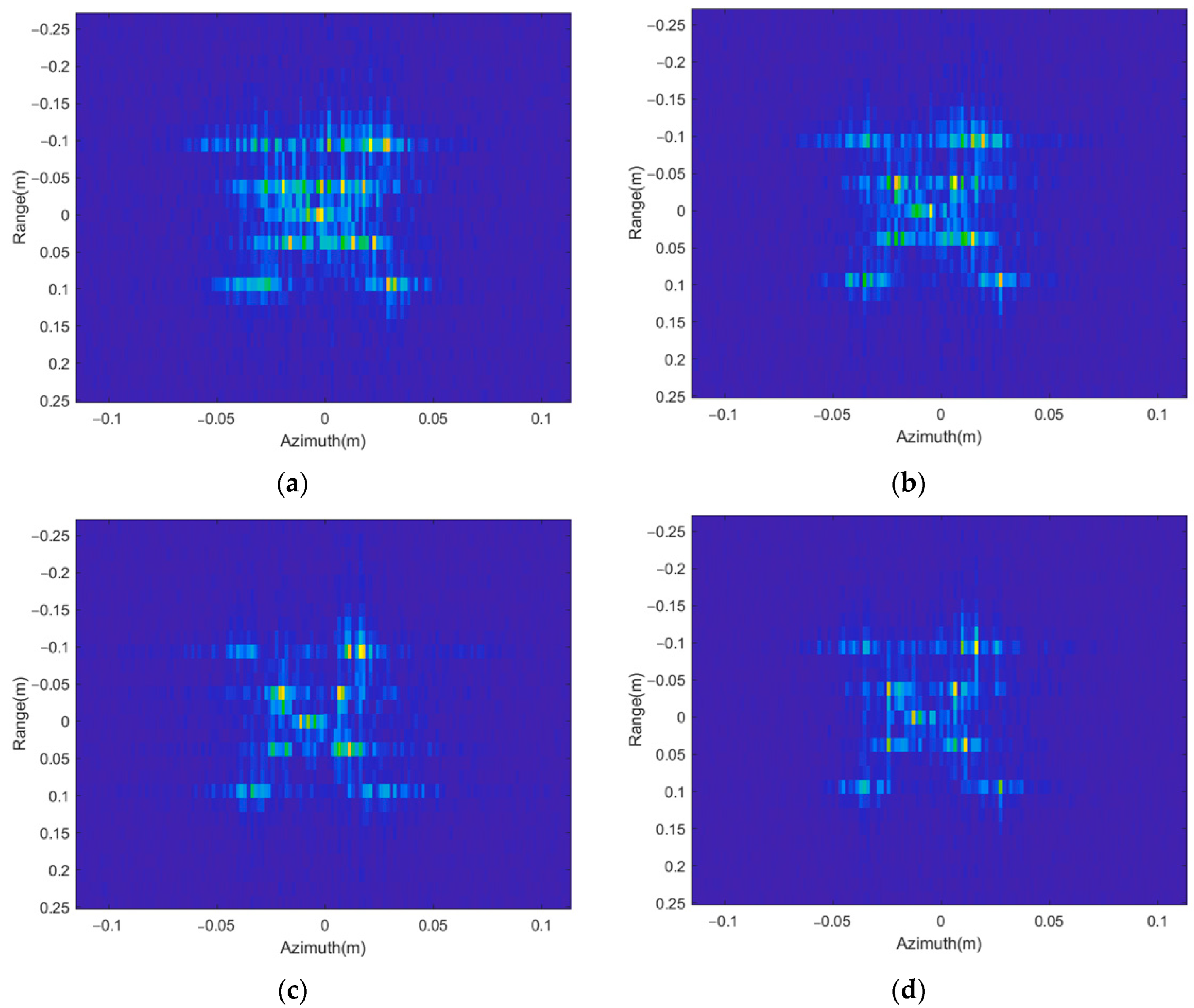
The results of processing the echo data using RD, PGA, PGMA and the proposed algorithm, respectively. The results obtained are shown in Figure 9.
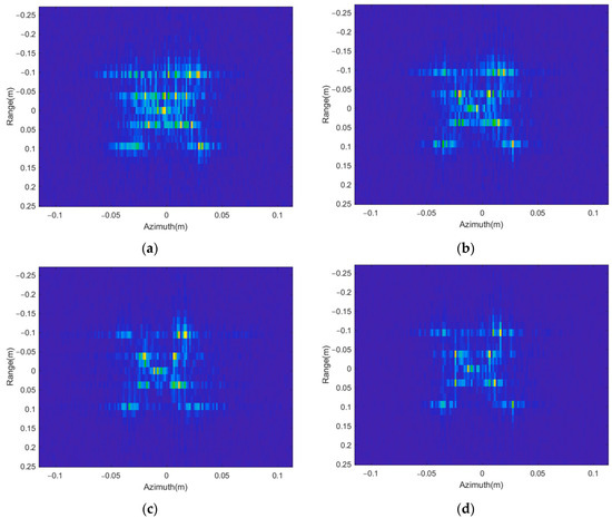
Figure 9.
Imaging results of measured data with different algorithms (a) RD; (b) PGA; (c) PGMA; (d) proposed algorithm.
Figure 9a shows the imaging results using the RD algorithm, where it can be observed that, due to the effect of target vibration, the image suffers from severe defocusing. The letter “X” is no longer distinguishable, and the defocusing degree varies across different target blocks, indicating the presence of a space-variant phase error. Figure 9b shows the imaging results using the PGA algorithm. It can be seen that the PGA algorithm achieves a certain degree of focus in the center of the target, but the four target blocks at the edges still exhibit some defocusing. Figure 9c shows the imaging results using the PGMA algorithm. Compared to the RD algorithm, most target blocks in the image are well-focused, but the target block located farthest from the center in the lower right corner still exhibits significant defocusing. Figure 9d presents the imaging results using the proposed algorithm. All target blocks in the image are clearly focused, indicating that the algorithm can effectively compensate for both space-variant and space-invariant phase errors.
Similarly, the results were quantitatively analyzed using image entropy and image contrast. The results are shown in Table 3. It can be seen that compared to the PGMA algorithm, the proposed algorithm reduces the image entropy by 0.16 and increases the contrast by 12%. The results indicate that the proposed algorithm achieves the best image quality, validating the effectiveness of the algorithm.
Table 3.
Image quality of real experimental data based on different algorithms.
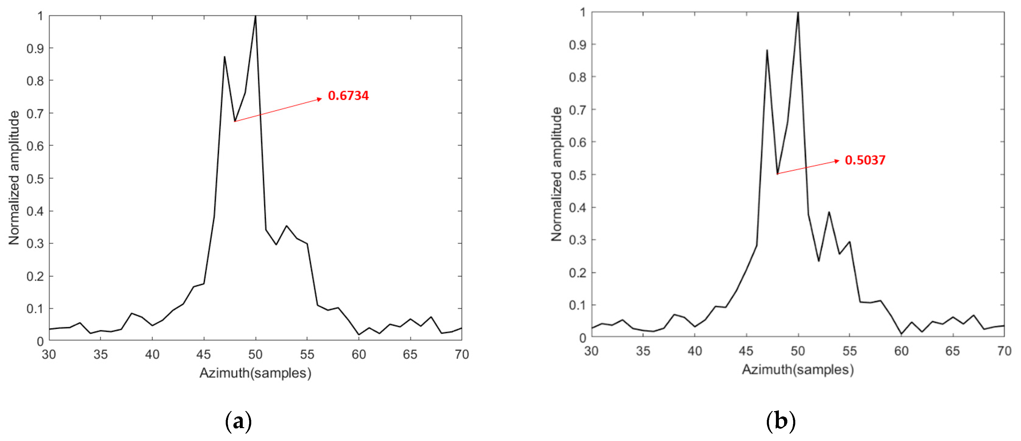
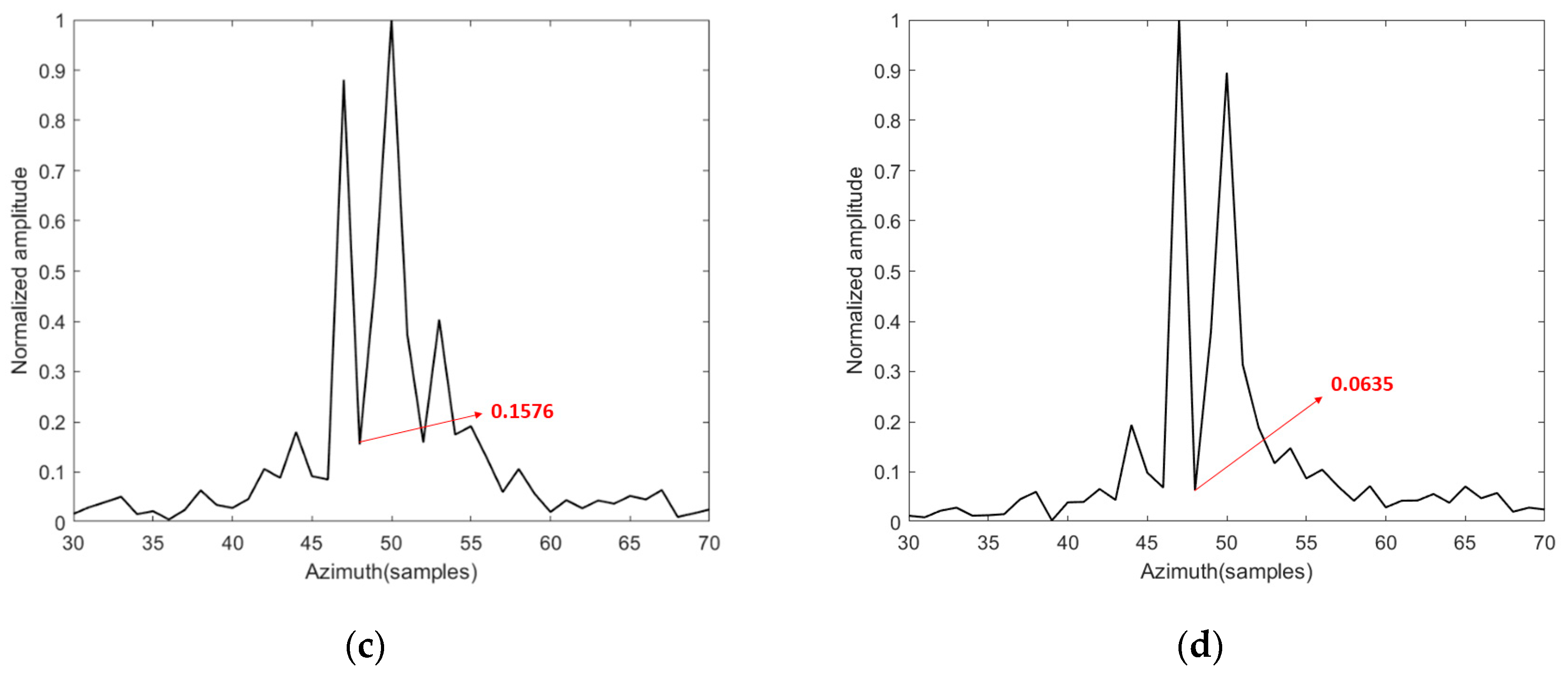
To further verify the compensation effect of the algorithm, we intercepted 100 pulses from the obtained echo data. The corresponding ladar azimuthal resolution at this point is approximately 0.8 cm, and the distance between the two target blocks at the second step of the “X” target is about 1.2 cm. The data were processed using the RD, PGA, PGMA, and proposed algorithms, and the target azimuthal profiles at the second step are shown in Figure 10.
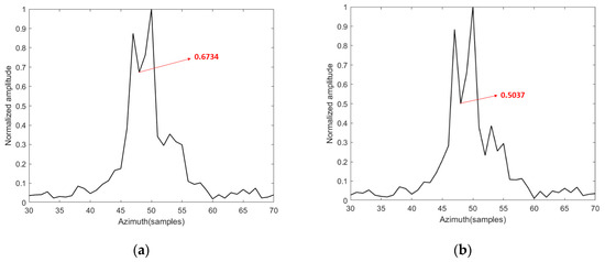
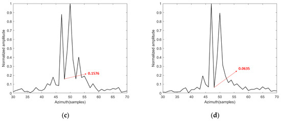
Figure 10.
Azimuthal profiles at the second step of the target (a) RD; (b) PGA; (c) PGMA; (d) proposed algorithm.
Figure 10 marks the normalized amplitude value at the minimum between two points. We characterize the discriminability of the two target blocks by the sum of amplitude differences between the target blocks and this minimum value. The calculated results for the four algorithms are 0.5275, 0.8658,1.5581, and 1.7681, respectively, demonstrating that the proposed algorithm achieves the highest distinction. Furthermore, a comparison of Figure 10a–d reveals noticeable sidelobes in Figure 10a–c, while Figure 10d shows effective sidelobe suppression, confirming that the proposed algorithm delivers optimal compensation performance and enhances azimuth resolution.
4. Discussion
This paper establishes an estimation model addressing both space-invariant and space-variant phase errors induced by satellite microvibration, and proposes an autofocus iterative compensation algorithm based on prior information and adaptive windowing. The processing results in Section 3 demonstrate that the proposed algorithm effectively compensates for both types of phase errors without limitations from phase error patterns or the presence of isolated scattering points in target scenes.
Quantitative evaluations across varying SNR conditions and real data experiment results reveal two key advantages:
- Superior Image Quality: The algorithm achieves optimal performance in both visual assessments and objective metrics (e.g., image contrast improves 22% at −5 dB SNR compared to conventional methods), validating its effectiveness and robustness.
- Enhanced Iterative Efficiency: Statistical analysis reveals that the proposed algorithm requires estimation for only approximately 30% of range cells per iteration, dramatically decreasing computational load. By incorporating prior information and adaptive windowing, the proposed algorithm reduces the number of iterations by 16–50% compared to the PGMA and PGA methods, while yielding superior image quality, as evidenced by Figure 6.
Notably, while PGMA requires manual parameter tuning (e.g., filtering thresholds, initial window width) for optimal results in different scenarios, our algorithm autonomously adapts windowing parameters across all SNR conditions, consistently delivering superior imaging outcomes. This self-adaptive capability significantly enhances its applicability to spaceborne ISAL systems requiring rapid imaging processing. These advancements address critical limitations in existing methods and establish a practical framework for vibration compensation in next-generation spaceborne ISAL systems.
5. Conclusions
Spaceborne ISAL imaging of satellites is significantly affected by microvibration during satellite operations, which introduces both space-variant and space-invariant phase errors, degrading image quality. In this paper, we develop a phase error estimation model for satellite vibration. Based on this model, we propose an improved vibration phase error compensation algorithm that utilizes a priori information and adaptive windowing. The algorithm holistically balances estimation accuracy with iteration efficiency, operating independently of the presence of prominent points in the target scene. By leveraging prior information, it selects optimal range cells for estimation, enhancing precision while reducing computational overhead per iteration. The integration of adaptive windowing mitigates clutter and noise interference, further improving both accuracy and robustness. The simulation results demonstrate that the proposed algorithm achieves optimal image quality and enhanced iterative efficiency within the SNR range of −10 to 6 dB, reducing the required iterations by 16–50%. Furthermore, in real data experiments, the algorithm reduces image entropy by 0.16 and improves image contrast by 12% compared with conventional methods. These results validate its superior capability in balancing the precision, robustness, and efficiency requirements for rapid spaceborne ISAL imaging. Future work will focus on FPGA-accelerated implementation for real-time onboard processing, while extending the framework to compensate for orbital motion perturbations and ultra-high-frequency microvibration in next-generation agile satellite imaging systems.
Author Contributions
Conceptualization, C.D. and C.C.; methodology, C.D.; software, C.D.; validation, C.D., C.C., H.L., X.W., J.T. and Z.F.; writing—original draft preparation, C.D. and C.C.; writing—review and editing, H.L., X.W., J.T. and Z.F. All authors have read and agreed to the published version of the manuscript.
Funding
This work was supported by the Natural Science Basis Research Program in Shaanxi Province of China (2024JC-YBMS-517).
Data Availability Statement
The next steps are also based on this research, therefore it is not appropriate to share procedures or data at this time.
Conflicts of Interest
The authors declare no conflicts of interest.
References
- Crouch, S.; Barber, Z.W. Laboratory demonstrations of interferometric and spotlight synthetic aperture ladar techniques. Opt. Express 2012, 20, 24237–24246. [Google Scholar] [CrossRef]
- Wang, N.; Wang, R.; Mo, D.; Li, G.; Zhang, K.; Wu, Y. Inverse synthetic aperture LADAR demonstration: System structure, imaging processing, and experiment result. Appl. Opt. 2018, 57, 230–236. [Google Scholar] [CrossRef] [PubMed]
- Rasouli, S.; Rajabi, Y. Investigation of the inhomogeneity atmospheric turbulence at day and night times. Opt. Laser Technol. 2016, 77, 40–50. [Google Scholar] [CrossRef]
- Abdukirim, A.; Ren, Y.; Tao, Z.; Liu, S.; Li, Y.; Deng, H.; Rao, R. Effects of Atmospheric Coherent Time on Inverse Synthetic Aperture Ladar Imaging through Atmospheric Turbulence. Remote Sens. 2023, 15, 2883. [Google Scholar] [CrossRef]
- Liu, L. Coherent and incoherent synthetic-aperture imaging LADARs and laboratory-space experimental demonstrations. Appl. Opt. 2013, 52, 579–599. [Google Scholar] [CrossRef] [PubMed]
- Wang, X.; Li, C.; Jia, J.; Wu, J.; Shu, R.; Zhang, L.; Wang, J. Angular micro-vibration of the Micius satellite measured by an optical sensor and the method for its suppression. Appl. Opt. 2021, 60, 1881–1887. [Google Scholar] [CrossRef] [PubMed]
- Wang, X.; Guo, L.; Li, Y.; Han, L.; Xu, Q.; Jing, D.; Li, L.; Xing, M. Noise-robust vibration phase compensation for satellite ISAL imaging by frequency descent minimum entropy optimization. IEEE Trans. Geosci. Remote Sens. 2022, 60, 5704417. [Google Scholar] [CrossRef]
- Pellizzari, C.J.; Bos, J.; Spencer, M.F.; Williams, S.; Williams, S.E.; Calef, B.; Senft, D.C. Performance characterization of phase gradient autofocus for inverse synthetic aperture LADAR. In Proceedings of the 2014 IEEE Aerospace Conference, Big Sky, MT, USA, 1–8 March 2014; pp. 1–11. [Google Scholar]
- Martorella, M.; Haywood, B.; Berizzi, F.; Dalle Mese, E. Performance analysis of an ISAR contrast-based autofocusing algorithm using real data. In Proceedings of the International Conference on Radar, Adelaide, SA, Australia, 3–5 September 2003; pp. 30–35. [Google Scholar]
- Kragh, T.J.; Kharbouch, A.A. Monotonic iterative algorithm for minimum-entropy autofocus. In Proceedings of the Adaptive Sensor Array Processing Workshop, Lexington, MA, USA, 6–7 June 2006; pp. 1147–1159. [Google Scholar]
- Hu, X.; Li, D.J. Vibration phases estimation based on multi-channel interferometry for ISAL. Appl. Opt. 2018, 57, 6481–6490. [Google Scholar] [CrossRef] [PubMed]
- Yin, H.; Guo, L.; Li, Y.; Han, L.; Xing, M.; Zeng, X. Varying Amplitude Vibration Phase Suppression Algorithm in ISAL Imaging. Remote Sens. 2022, 14, 1122. [Google Scholar] [CrossRef]
- Song, Z.; Mo, D.; Wang, N.; Li, B.; Shao, Y.; Tan, R. Inverse synthetic aperture ladar autofocus imaging algorithm for microvibrating satellites based on two prominent points. Appl. Opt. 2019, 58, 6775–6783. [Google Scholar] [CrossRef]
- Song, Z.; Mo, D.; Li, R.; Wang, Y.; Shao, Y.; Tan, R. Phase gradient matrix autofocus for ISAL space-time-varied phase error correction. IEEE Photon. Technol. Lett. 2020, 32, 353–356. [Google Scholar] [CrossRef]
- Levtov, V.L.; Romanov, V.V.; Babkin, E.V.; Ivanov, A.I.; Stazhkov, V.M.; Sazonov, V.V. Measurement of vibration microaccelerations onboard the Mir orbital station using the VM-09 system of accelerometers. Cosmic Res. 2004, 42, 165–177. [Google Scholar] [CrossRef]
- Riaboukha, S.B.; Kiselev, S.V. Some Features of Vibrational Perturbations onboard the MirOrbital Station. Cosmic Res. 2001, 39, 120–125. [Google Scholar] [CrossRef]
- Wu, L.; Wei, X.; Yang, D.; Wang, H.; Li, X. ISAR Imaging of Targets With Complex Motion Based on Discrete Chirp Fourier Transform for Cubic Chirps. IEEE Trans. Geosci. Remote Sens. 2012, 50, 4201–4212. [Google Scholar] [CrossRef]
- Xi, L.; Guosui, L.; Ni, J. Autofocusing of ISAR images based on entropy minimization. IEEE Trans. Aerosp. Electron. Syst. 1999, 35, 1240–1252. [Google Scholar] [CrossRef]
- Wittig, M.E.; Holtz, L.V.; Tunbridge, D.E.L.; Vermeulen, H.C. In-orbit measurements of microaccelerations of ESA’s communication satellite OLYMPUS. In Proceedings of the Free-Space Laser Communication Technologies II, Los Angeles, CA, USA, 1 July 1990; pp. 205–214. [Google Scholar]
- Toyoshima, M.; Takayama, Y.; Kunimori, H.; Jono, T.; Yamakawa, S. In-orbit measurements of spacecraft microvibrations for satellite laser communication links. Opt. Eng. 2010, 49, 083604. [Google Scholar] [CrossRef]


Disclaimer/Publisher’s Note: The statements, opinions and data contained in all publications are solely those of the individual author(s) and contributor(s) and not of MDPI and/or the editor(s). MDPI and/or the editor(s) disclaim responsibility for any injury to people or property resulting from any ideas, methods, instructions or products referred to in the content. |
© 2025 by the authors. Licensee MDPI, Basel, Switzerland. This article is an open access article distributed under the terms and conditions of the Creative Commons Attribution (CC BY) license (https://creativecommons.org/licenses/by/4.0/).