Evaluating the Performance of Satellite-Derived Soil Moisture Products Across South America Using Minimal Ground-Truth Assumptions in Spatiotemporal Statistical Analysis

Abstract

South America (SA) features diverse land cover types and varied climate conditions, both of which significantly influence the variability of soil moisture (SMO). Obtaining ground-truth measurements for SMO is often costly and labor-intensive, and the limited number of ground SMO stations in SA further complicates the evaluation of satellite-derived SMO products. In this work, we proposed an approach that integrates some statistical methods to assess the reliability of Soil Moisture Active Passive (SMAP), the H113 dataset from the Advanced Scatterometer (ASCAT), and Soil Moisture and Ocean Salinity (SMOS) satellite-derived SMO products in SA from 14 May 2015 to 31 December 2016. The integrated methods are error metrics (correlation (R), bias, and ubiased root mean square error (ubRMSE)), Triple Collocation Method (TCM), and Hovmöller diagrams. ERA5 and GLDAS-Noah SM products were used as references for validation. The quality of SMO products was assessed by considering environmental variables, including land cover, vegetation density, and precipitation, within the different climate zones of SA. The results presented that SMAP overall outperforms SMOS and ASCAT, with the highest average correlation (0.55 with GLDAS and 0.61 with ERA5), slight average bias (−0.058 with GLDAS and −0.014 with ERA5), and lowest average ubRMSE (0.045 with GLDAS and 0.041 with ERA5). In arid, semi-arid, and moderate vegetation regions, the SMAP satellite outperforms SMOS and ASCAT, achieving better statistics values with GLDAS and ERA5 datasets, and achieving low error variance and high S/N in the TCM analysis. While the ASCAT H113 product showed good performance, which makes it a good alternative to SMAP, it still has limitations in more dense vegetation regions. SMOS showed the lowest performance across SA, especially in the Amazon basin. The Amazon basin emerges as a critical region where all SMO products displayed a significant SMO variability; however, SMAP showed slightly better results than ASCAT and SMOS. In the absence of ground truths, the proposed approach provides a better evaluation of satellite SMO products. Meanwhile, it provides new spatiotemporal statistical insights into satellite SMO retrieval performance evaluation within diverse climate zones of SA. This research provides valuable guidance for improving SMO monitoring and agricultural management in tropical and semi-arid ecosystems.

1. Introduction

Soil moisture (SMO) is an essential parameter for hydrological modeling, agricultural productivity, weather prediction, and climate change influence; additionally, it is important for applications such as drought monitoring and flood forecasting [1,2]. The conventional ground methods to measure SMO include gravimetric techniques, lysimeters, and soil sensors. But these methods still face limitations, such as high costs, spatial limitations, and logistical restrictions, especially for large regions [3,4]. In contrast, remote sensing (RS) using microwave passive or active sensors is considered the most significant source for SMO observations at a global scale [5]. Microwave passive remote sensing, which operates at L, C, and X bands, and active RS, which typically operates at the C band, have both been extensively used to observe SMO [6]. The common passive satellites for retrieving SMO are AMSR2, SMOS, and SMAP. Meanwhile, the ASCAT is an active sensor mounted on several satellites, including Metop-A, Metop-B, and Metop-C [7,8].

The soil-moisture retrievals from microwave instruments are prone to uncertainty due to the noise in the measuring equipment, exaggerations, assumption violations, and miscalibrations in retrieval models, which are used to retrieve SMO information from raw satellite data. Therefore, before using SMO data, the analysis and interpretation of their accuracy should be considered. Although the SMAP, SMOS, and ASCAT missions have a significant development in monitoring SMO on spatiotemporal coverage, these satellites still face challenges that can significantly affect the accuracy and reliability of SMO retrievals, including surface roughness, vegetation influence, freeze–thaw cycles, and issues associated with data assimilation and spatial resolution, especially in areas with heterogeneous landscapes [2,9,10,11,12].

The standard error metrics include correlation (R), bias, and unbiased root mean square error (ubRMSE)) were used extensively in evaluating satellite SMO products against either in situ measurements or model/reanalysis data. Ground SMO measurements are the most common and robust method to check the accuracy of SMO products. However, the unidentical in situ observations and the regions captured by satellite sensors overall, result in increasing error, which frequently exceeds the real estimate of errors in retrieval for the product undergoing validation [13,14,15,16]. Furthermore, the in situ measurements available on small zones of the world land surface, thus, are insufficient for thorough validation of satellite SMO products across all climate conditions and land cover types [17].

Comparing satellite SMO retrievals with land surface models is another method of assessing satellite products [18]. Although these models are available worldwide and share a similar spatial resolution, they contain substantial modeling errors, and their quality is frequently not well-characterized [19]. Furthermore, unlike standard error metrics, the TCM is a statistical error model that can assess satellite SMO datasets without requiring an extra reference dataset. Although TCM analysis has been identified as one of the most significant techniques for evaluating error structures in satellite SMO datasets, there is still some restriction because it depends on some assumptions. The assumptions of the TCM include homogeneity of data both spatially and temporally, errors stationarity, independence of error structures, the presence of a linear relationship among the three estimates, and the non-existence of systematic biases. These assumptions, which are often interpreted as a constraint that is specific to TCM analysis, are often seen to be common for other traditional performances [20,21]. Hovmöller diagrams were initially developed by Ernest Hovmöller in 1948; these diagrams are essential in atmospheric and oceanic fields for spatiotemporal variability visualization and recognizing climate anomalies. Hovmöller diagrams were utilized to study SMO dynamics and their anomalies by plotting SMO variations across longitude or latitude over time [14,22,23].

South America (SA)’s features are characterized by diverse climate and land surface conditions [24], which influence the regional SMO dynamics. Moreover, the limited number of ground-based SMO stations [17,25] across SA presents a challenge for assessing the reliability of SMO products. Traditional assessment approaches require dense networks of ground-based sensors to validate satellite SMO products [13,26,27,28], which are frequently unavailable across SA land covers. In this work, minimal ground-truth assumptions aim to reduce the dependence on extensive in situ SMO measurements or rigorous assumptions about temporal consistency, spatial distribution, or accuracy of ground-based SMO validation data, through spatiotemporal statistical analysis. Therefore, this research adopts an approach to assess the reliability of ASCAT H113, SMAP, SMOS, and SMO datasets across SA by integrating some statistical methods. The integrated methods include standard error metrics (R, bias, ubRMSE), TCM, and Hovmöller diagrams. First, the error metrics were used to validate satellite SMO products versus both GLDAS-Noah and ERA5 SMO datasets. Second, TCM was applied to estimate error patterns and the signal-to-noise ratio (S/N) of SMO products. Third, Hovmöller diagrams were utilized to identify anomalies and trends in the SMO products. The quality of the SMO products was assessed by considering environmental variables, including land cover, vegetation density, and rainfall, within the different climate zones of SA. The proposed approach will provide a comprehensive assessment of the reliability of satellite SMO products across SA, as will be discussed later.

2. Study Area and Datasets

2.1. Study Area

South America, as shown in Figure 1, is located between longitudes 35°W to 85°W and latitudes 25°N to 56°S. SA has various land covers and varied climate conditions [29] (see Figure 1a,b) which reflect the regional SMO dynamic. Based on the Köppen–Geiger climate classification [30], SA is a home to a variety of climate zones, as shown in Figure 1b, including tropical, temperate, dry, and polar climates. A tropical climate zone with abundant rainfall and high temperatures covers much of Northern SA, including the Amazon basin, where both the tropical rainforest and tropical savanna dominate. The dry climate zone includes hot and cold climates for both desert and semi-arid regions, which are concentrated in the cold desert of the Andes (BWk), the hot Atacama Desert in Chile (BWh), the hot semi-arid regions in Northern Chile and parts of Argentina (BSh), and the cold of semi-arid areas in Central Argentina (BSk). The temperate climate zone is characterized by moderate temperatures and distinct seasonal patterns, which are represented in the humid subtropical climate (Cfa) in the regions of Northern Argentina and Southern Brazil, the oceanic climate (Cfb) in the region of southern Chile, and the subpolar oceanic climate (Cfc) in the southernmost regions of Chile and Argentina. Also, the Mediterranean climate (Csb and Csc) is present in Central Chile and higher-altitude regions. Also, the subtropical highland climates (Cwa, Cwb, and Cwc) are in the Andes and southern parts of Brazil. The polar climate (ET) is in the highest areas of the Andes and the southernmost regions of Chile and Argentina (Patagonia and Tierra del Fuego). These various climates support a range of ecosystems across SA, especially in the southern regions. Moreover, the performance of satellite SMO products is still not fully understood on the regional scale, especially across SA, due to less representative in situ data [17] (see Figure 1b).

To understand the reliability of satellite SMO products across South America, the average Normalized Difference Vegetation Index (NDVI) values and precipitation amounts across land cover types of SA were calculated from 14 May 2015 to 31 December 2016, as shown in Figure 2. Moreover, the correlation between NDVI, rainfall amounts, and land cover types in SA are determined is shown in Figure 3. South America has a varied land cover from barren deserts in the southwestern regions (dry climate zones, as shown in Figure 1b, to dense forests in the Amazon basin (tropical climate zone as shown in Figure 1b). In the desert regions of South America, the calculated average NDVI value was found to be a very small value, reflecting sparse vegetation and minimal rainfall amounts (see Figure 2 and Figure 3). Also, in the shrublands of the dry climate zones (see Figure 1a), both average NDVI value and rainfall amount are low. Meanwhile, the grasslands within the temperate and tropical climate zones (see Figure 1a) exhibit moderate rainfall amounts and corresponding NDVI values. In contrast, in croplands, savannas, and forests (see Figure 2 and Figure 3), influenced by tropical and temperate climate zones (see Figure 1a), the rainfall amounts and average NDVI values are significantly higher, indicating dense vegetation and productive ecosystems. These results emphasize a relationship between rainfall and vegetation density across land covers within climate zones of SA. This relationship was used to provide significant insights into how the interaction between these environmental variables affects the satellite SMO product’s performance across SA, as we will discuss later.

2.2. Microwave Passive and Active SMO Datasets

In January 2015, NASA launched the SMAP satellite, which carries both an L-band radar (1.26 GHz) and L-band radiometer (1.41 GHz). Only the SMAP radiometer can provide observations, because the radar equipment stopped working a few months after launching, due to an irreversible hardware failure. SMAP observes the earth at solar-based times of 06:00 and 18:00 during descending and ascending orbits, respectively. The SMAP satellite was developed to retrieve SMO with an accuracy of 0.04, particularly in the regions with low-to-moderate vegetation [31,32]. In this work, the ascending and descending observations of the SMAP L3 (V6) radiometer with a 36 km resolution were used.

The SMOS satellite mission has been operating at L band (1.4 GHz) and launched by the ESA since 2009. SMOS can revisit a region of the earth every 2–3 days at solar-based times of 6:00 and18:00 during ascending and descending orbits, respectively. The algorithm of retrieving SMOS SMO is L-band Microwave Emission of the Biosphere (L-MEB) [27,33,34]. In this research, the descending and ascending SMO measurements of SMOS L3 with a 25 km resolution were evaluated.

ASCAT is an active radar operating at C-band frequency of 5.255 GHz, using the TU Wien algorithm, and is employed on several satellites, including the Metop-A, Metop-B, and Metop-C. In this work, the ASCAT H113 SMO dataset, with a spatial resolution of 12.5 km, was used from the EUMETSAT data center as part of the H-SAF to generate operational SMO products. The H113 product is produced based on the Level 1b backscatter products from Metop-A and Metop-B [35,36,37].

2.3. Reference SMO Datasets

The analysis GLDAS-Noah was developed by NASA and NOAA. The GLDAS model offers time-series (3 h) SMO data with a spatial resolution of 0.25° for four layers at different depths [38]. GLDAS-Noah has been widely validated and utilized across different different zones and scales, indicating its reliability in simulating SMO, hydrological processes, and drought monitoring. GLDAS-Noah showed better than CLM and VIC in representing SMO dynamics and drought detection. Moreover, GLDAS-Noah was used widely as a reference in the validation and fusion of active and passive SMO retrievals [39,40,41,42,43]. In this work, the top (0–10 cm) SMO available from GLDAS-Noah (V2.1), was utilized as a reference to validate the SMO products and as one of the TCM products.

In this study, the daily average SMO, with a spatial resolution of 0.25° from the ERA5 reanalysis, was utilized to evaluate the efficacy of satellite SMO datasets in SA. The European Centre developed the global ERA5 atmospheric reanalysis for Medium-Range Weather Forecasts (ECMWFs). The examination of ERA5 indicates its reliability in the lack or absence of in situ measurements [44,45]. ERA5 dataset can be accessed through https://cds.climate.copernicus.eu/datasets; accessed on 15 January 2024.

2.4. Ancillary Datasets

The Land Cover MCD12Q1 product (V6), featuring a spatial resolution of 500 m, was obtained for 2016 to assess the performance of SMO products across various land cover types in SA. This product offers an annual global land cover map from 2001 to the current date [46].

The monthly NDVI product from MODIS (The MOD13C2 0.05-Deg, V6) was used from 14 May 2015 to 31 December 2016 to check the state of vegetation density for various types of land cover. This helps in understanding the reliability of SMO products across SA.

The monthly Global Precipitation Climatology Centre (GPCC) dataset, featuring a spatial resolution of 0.25°, was used to interpret the results of SMO products’ assessment in SA [47]. The unit of rainfall measurement in this product is mm/month.

Moreover, the Köppen–Geiger climate classification dataset (V2) with a resolution of 1 km was used to assess the performances of satellite SMO products within the different climate zones of South America. This dataset is developed on high-resolution, observation-founded climatologies for the period from 1991 to 2020 [30].

3. Methods

In this work, to overcome the challenges of fewer ground SMO stations in SA [17,25] we proposed a comprehensive approach, illustrated in Figure 4, to examine the performance of SMO products across the SA continent based on spatiotemporal statistical analysis. The used statistical methods in the proposed approach are standard error metrics (R, bias, ubRMSE), TCM for error estimation and signal-to-noise ratio (S/N), and Hovmöller diagrams for analyzing the spatiotemporal dynamics of SMO across satellite products. ERA5 and GLDAS-Noah SM products were used as references for validation. The performance of satellite SMO products was investigated considering environmental variables within diverse climate zones of South America. The proposed approach is based on minimal ground-truth assumptions and will reduce the dependence on extensive in situ SMO measurements or rigorous assumptions about temporal consistency, spatial distribution, or accuracy of ground SMO validation data. The used approach will be covered in the following subsections: data preprocessing, error metrics, triple collocation error model, and Hovmöller diagrams.

3.1. Data Preprocessing

In this study, the quality control was performed on all SMO products to exclude unreliable SMO retrievals, according to the conditions set by the algorithm developers or documents outlining the theoretical foundation of the algorithm, as follows:

• SMAP SMO values were filtered for SMO < 0.02 m³/m³, SMO > 0.50 m³/m³, and when recommended retrieval flag. The daily average descending and ascending SMO was resampled to 25 km using the nearest-neighbor method [48].
• SMOS SMO values were filtered to eliminate unreliable SMO retrievals based on RFI probability > 0.2, Data Quality Index < 0.1, and SMO not within the range of 0–0.6 m³/m³ [26]. The daily average descending and ascending of SMOS SMO retrievals were calculated.
• ASCAT H113 SMO retrievals were masked using the information of Surface State Flag (SSF) for snow/frozen probability and retrieval error > 50%. SMO was resampled to 25 km using the nearest-neighbor resampling algorithm. SMO was transformed from the degree of saturation (%) to m³/m³ using soil porosity estimates from the database of world soil for the upper layer (0–40cm) [14,49] and available through the ESA website.
• GLDAS-Noah ERA5 SMO data were used when the temperature of the topsoil was above 0 °C [50].

Moreover, to avoid frozen probability, passive satellite SMO observations were only used at temperatures more than 0 °C. The precipitation amounts value from GPCC product was computed across SA from 14 May 2015 to 31 December 2016. Also, the average NDVI values were calculated for the temporal period of study across SA.

3.2. Error Metrics

In this work, the satellite SMO datasets were assessed against ERA5 and GLDAS-Noah SMO datasets by using bias, ubRMSE, and the R [51]. These metrics were computed by utilizing the following formulas:

$$\mathrm{B}\mathrm{i}\mathrm{a}\mathrm{s}=\mathrm{E}\left[{\mathrm{S}\mathrm{M}\mathrm{O}}_{\mathrm{s}}\left(\mathrm{t}\right)\right]-\mathrm{E}\left[{\mathrm{S}\mathrm{M}\mathrm{O}}_{\mathrm{r}}\left(\mathrm{t}\right)\right]$$

(1)

$$\mathrm{u}\mathrm{b}\mathrm{R}\mathrm{M}\mathrm{S}\mathrm{E}=\sqrt{{\mathrm{E}\left[\left({\mathrm{S}\mathrm{M}\mathrm{O}}_{\mathrm{s}}\left(\mathrm{t}\right)-\mathrm{E}\left[{\mathrm{S}\mathrm{M}\mathrm{O}}_{\mathrm{s}}\left(\mathrm{t}\right)\right]\right)-(\mathrm{S}{\mathrm{M}\mathrm{O}}_{\mathrm{r}}\left(\mathrm{t}\right)-\mathrm{E}\left[{\mathrm{S}\mathrm{M}\mathrm{O}}_{\mathrm{r}}\left(\mathrm{t}\right)\right])\right]}^2}$$

(2)

$$\mathrm{R}={\displaystyle \frac{\mathrm{E}\left[\left({\mathrm{S}\mathrm{M}\mathrm{O}}_{\mathrm{s}}\left(\mathrm{t}\right)-\mathrm{E}\left[{\mathrm{S}\mathrm{M}\mathrm{O}}_{\mathrm{s}}\left(\mathrm{t}\right)\right]\right)\left({\mathrm{S}\mathrm{M}\mathrm{O}}_{\mathrm{r}}\left(\mathrm{t}\right)-\mathrm{E}\left[{\mathrm{S}\mathrm{M}\mathrm{O}}_{\mathrm{r}}\left(\mathrm{t}\right)\right]\right)\right]}{{\mathsf{\sigma }}_{\mathrm{s}}{\mathsf{\sigma }}_{\mathrm{r}}}}$$

(3)

where $\mathrm{E}[.]$ denotes the computation of mean values; t represents the observation time; SMO_s(t) refers to a satellite SMO retrieval at time t; and SMO_r(t) symbolizes the reference SMO product, either GLDAS or ER5, at the same time t. The symbols ${\mathsf{\sigma }}_{\mathrm{r}}$ and ${\mathsf{\sigma }}_{\mathrm{s}}$ represent the standard deviation of reference data and satellite SMO retrieval data, respectively. The R was determined at a p-value of less than 0.05, indicating a high level of significance.

3.3. Triple Collocation Method

In this research work, the TCM was also used to evaluate the reliability of SMO products in South America. The TCM is considered a promising method for validating satellite-based SMO. In the analysis of TCM, satellite SMO products’ accuracy can be estimated without ground truths as conventional metrics [21]. A linear error model displayed in Equation (4) is considered the basis for TCM.

$${\mathrm{S}\mathrm{M}\mathrm{O}}_{\mathrm{s}\mathrm{i}}={\mathsf{\alpha }}_{{\mathrm{S}\mathrm{M}\mathrm{O}}_{\mathrm{s}\mathrm{i}}}+{\mathsf{\beta }}_{{\mathrm{S}\mathrm{M}\mathrm{O}}_{\mathrm{s}\mathrm{i}}}{\mathrm{S}\mathrm{M}\mathrm{O}}_{\mathrm{t}}+{\mathsf{\epsilon }}_{{\mathrm{S}\mathrm{M}\mathrm{O}}_{\mathrm{s}\mathrm{i}}}$$

(4)

where ${\mathrm{S}\mathrm{M}\mathrm{O}}_{\mathrm{t}}$ symbolizes the unknown true SMO; $\mathrm{S}{\mathrm{M}\mathrm{O}}_{\mathrm{s}\mathrm{i}}$ ∈ [${\mathrm{S}\mathrm{M}\mathrm{O}}_{\mathrm{s}1}$, ${\mathrm{S}\mathrm{M}\mathrm{O}}_{\mathrm{s}2}$, ${\mathrm{S}\mathrm{M}\mathrm{O}}_{\mathrm{s}3}$] are three spatiotemporally collocated datasets; ${\mathsf{\beta }}_{{\mathrm{S}\mathrm{M}\mathrm{O}}_{\mathrm{s}\mathrm{i}}}$ and ${\mathsf{\alpha }}_{{\mathrm{S}\mathrm{M}\mathrm{O}}_{\mathrm{s}\mathrm{i}}}$ denote multiplicative biases and systematic additive of ${\mathrm{S}\mathrm{M}\mathrm{O}}_{\mathrm{s}\mathrm{i}}$ product concerning the true value; and ${\mathsf{\epsilon }}_{{\mathrm{S}\mathrm{M}\mathrm{O}}_{\mathrm{s}\mathrm{i}}}$ symbolizes additive zero-mean random noise [21,52]. The S/N and error variance of SMO datasets considering the assumptions of TCM were calculated using Equation (5) to Equation (11) [21]:

$${\mathrm{V}}_{{\mathsf{\epsilon }}_{\left({\mathrm{S}\mathrm{M}\mathrm{O}}_{\mathrm{s}1}\right)}}={\mathrm{V}}_{\left({\mathrm{S}\mathrm{M}\mathrm{O}}_{\mathrm{s}1}\right)}-{\displaystyle \frac{{\mathrm{C}\mathrm{O}\mathrm{V}}_{(\mathrm{S}{\mathrm{M}\mathrm{O}}_{\mathrm{s}1},{\mathrm{S}\mathrm{M}\mathrm{O}}_{\mathrm{s}2})}{\mathrm{C}\mathrm{O}\mathrm{V}}_{(\mathrm{S}{\mathrm{M}\mathrm{O}}_{\mathrm{s}1},{\mathrm{S}\mathrm{M}\mathrm{O}}_{\mathrm{s}3})}}{{\mathrm{C}\mathrm{O}\mathrm{V}}_{({\mathrm{S}\mathrm{M}\mathrm{O}}_{\mathrm{s}2},{\mathrm{S}\mathrm{M}\mathrm{O}}_{\mathrm{s}3})}}}$$

(5)

$${\mathrm{V}}_{{\mathsf{\epsilon }}_{\left({\mathrm{S}\mathrm{M}\mathrm{O}}_{\mathrm{s}2}\right)}}={\mathrm{V}}_{\left(\mathrm{S}{\mathrm{M}\mathrm{O}}_{\mathrm{s}2}\right)}-{\displaystyle \frac{{\mathrm{C}\mathrm{O}\mathrm{V}}_{(\mathrm{S}{\mathrm{M}\mathrm{O}}_{\mathrm{s}2},{\mathrm{M}}_{\mathrm{s}1})}{\mathrm{C}\mathrm{O}\mathrm{V}}_{(\mathrm{S}{\mathrm{M}\mathrm{O}}_{\mathrm{s}2},{\mathrm{S}\mathrm{M}\mathrm{O}}_{\mathrm{s}3})}}{{\mathrm{C}\mathrm{O}\mathrm{V}}_{({\mathrm{S}\mathrm{M}\mathrm{O}}_{\mathrm{s}1},{\mathrm{S}\mathrm{M}\mathrm{O}}_{\mathrm{s}3})}}}$$

(6)

$${\mathrm{V}}_{{\mathsf{\epsilon }}_{\left({\mathrm{M}}_{\mathrm{s}3}\right)}}={\mathrm{V}}_{\left({\mathrm{M}}_{\mathrm{s}3}\right)}-{\displaystyle \frac{{\mathrm{C}\mathrm{O}\mathrm{V}}_{({\mathrm{S}\mathrm{M}\mathrm{O}}_{\mathrm{s}3},\mathrm{S}{\mathrm{M}\mathrm{O}}_{\mathrm{s}2})}{\mathrm{C}\mathrm{O}\mathrm{V}}_{({\mathrm{S}\mathrm{M}\mathrm{O}}_{\mathrm{s}3},{\mathrm{S}\mathrm{M}\mathrm{O}}_{\mathrm{s}1})}}{{\mathrm{C}\mathrm{O}\mathrm{V}}_{({\mathrm{S}\mathrm{M}\mathrm{O}}_{\mathrm{s}2},{\mathrm{S}\mathrm{M}\mathrm{O}}_{\mathrm{s}1})}}}$$

(7)

where ${\mathrm{V}}_{{\mathsf{\epsilon }}_{\left({\mathrm{S}\mathrm{M}\mathrm{O}}_{\mathrm{s}1}\right)}}$, ${\mathrm{V}}_{{\mathsf{\epsilon }}_{\left({\mathrm{S}\mathrm{M}\mathrm{O}}_{\mathrm{s}2}\right)}}$, and ${\mathrm{V}}_{{\mathsf{\epsilon }}_{\left({\mathrm{S}\mathrm{M}\mathrm{O}}_{\mathrm{s}3}\right)}}$ denote error variance of satellite SMO datasets; and ${\mathrm{S}\mathrm{M}\mathrm{O}}_{\mathrm{s}1}$, ${\mathrm{S}\mathrm{M}\mathrm{O}}_{\mathrm{s}2}$, and ${\mathrm{S}\mathrm{M}\mathrm{O}}_{\mathrm{s}3}$ symbolize the independent SMO products in a triplet.

$${(\mathrm{S}/\mathrm{N})}_{\left({\mathrm{S}\mathrm{M}\mathrm{O}}_{\mathrm{s}1}\right)}={\displaystyle \frac{{\mathrm{C}\mathrm{O}\mathrm{V}}_{({\mathrm{S}\mathrm{M}\mathrm{O}}_{\mathrm{s}1},{\mathrm{S}\mathrm{M}\mathrm{O}}_{\mathrm{s}2})}{\mathrm{C}\mathrm{O}\mathrm{V}}_{({\mathrm{S}\mathrm{M}\mathrm{O}}_{\mathrm{s}1},{\mathrm{S}\mathrm{M}\mathrm{O}}_{\mathrm{s}3})}}{{\mathrm{V}}_{\left({\mathrm{S}\mathrm{M}\mathrm{O}}_{\mathrm{s}1}\right)}{\mathrm{C}\mathrm{O}\mathrm{V}}_{({\mathrm{S}\mathrm{M}\mathrm{O}}_{\mathrm{s}2},{\mathrm{S}\mathrm{M}\mathrm{O}}_{\mathrm{s}3})}}}$$

(8)

$${(\mathrm{S}/\mathrm{N})}_{\left({\mathrm{S}\mathrm{M}\mathrm{O}}_{\mathrm{s}2}\right)}={\displaystyle \frac{{\mathrm{C}\mathrm{O}\mathrm{V}}_{({\mathrm{S}\mathrm{M}\mathrm{O}}_{\mathrm{s}2},{\mathrm{S}\mathrm{M}\mathrm{O}}_{\mathrm{s}1})}{\mathrm{C}\mathrm{O}\mathrm{V}}_{({\mathrm{S}\mathrm{M}\mathrm{O}}_{\mathrm{s}2},{\mathrm{S}\mathrm{M}\mathrm{O}}_{\mathrm{s}3})}}{{\mathrm{V}}_{\left({\mathrm{S}\mathrm{M}\mathrm{O}}_{\mathrm{s}2}\right)}{\mathrm{C}\mathrm{O}\mathrm{V}}_{({\mathrm{S}\mathrm{M}\mathrm{O}}_{\mathrm{s}1},{\mathrm{S}\mathrm{M}\mathrm{O}}_{\mathrm{s}3})}}}$$

(9)

$${(\mathrm{S}/\mathrm{N})}_{\left({\mathrm{S}\mathrm{M}\mathrm{O}}_{\mathrm{s}3}\right)}={\displaystyle \frac{{\mathrm{C}\mathrm{O}\mathrm{V}}_{({\mathrm{S}\mathrm{M}\mathrm{O}}_{\mathrm{s}3},{\mathrm{S}\mathrm{M}\mathrm{O}}_{\mathrm{s}2})}{\mathrm{C}\mathrm{O}\mathrm{V}}_{({\mathrm{S}\mathrm{M}\mathrm{O}}_{\mathrm{s}3},{\mathrm{S}\mathrm{M}\mathrm{O}}_{\mathrm{s}1})}}{{\mathrm{V}}_{\left({\mathrm{S}\mathrm{M}\mathrm{O}}_{\mathrm{s}3}\right)}{\mathrm{C}\mathrm{O}\mathrm{V}}_{({\mathrm{S}\mathrm{M}\mathrm{O}}_{\mathrm{s}2},{\mathrm{S}\mathrm{M}\mathrm{O}}_{\mathrm{s}1})}}}$$

(10)

$$(\mathrm{S}/\mathrm{N})\left[\mathrm{d}\mathrm{b}\right]=10\mathrm{l}\mathrm{o}\mathrm{g}\left({(\mathrm{S}/\mathrm{N})}_{\left({\mathrm{S}\mathrm{M}\mathrm{O}}_{\mathrm{s}\mathrm{i}}\right)}\right)$$

(11)

where ${(\mathrm{S}/\mathrm{N})}_{\left({\mathrm{S}\mathrm{M}\mathrm{O}}_{\mathrm{s}1}\right)}$, ${(\mathrm{S}/\mathrm{N})}_{\left({\mathrm{S}\mathrm{M}\mathrm{O}}_{\mathrm{s}2}\right)}$, and ${(\mathrm{S}/\mathrm{N})}_{\left({\mathrm{S}\mathrm{M}\mathrm{O}}_{\mathrm{s}3}\right)}$ represent the signal-to-noise ratio of SMO datasets; V represent the variance of satellite data error; and COV denotes the covariance of the two SMO products. The S/N was calculated in decibels [db], which facilitates in the understanding of S/N; evidently, more information about S/N and the meaning of different S/N [db] values is there [21].

TCM supposes independent errors; hence, to avoid the partially correlated errors that may be caused because of similar derivations between datasets, we chose SMO datasets with varying derivations as much as possible [13]. This may occur with SMOS and SMAP radiometer products. Therefore, we performed two TCM computations: one using SMOS, ASCAT H113, and ERA5; and one using SMAP, ASCAT H113, and ERA5. The TCM statistics for ASCAT H113 were computed from the triplet containing the SMOS product since the frequency of ASCAT is not closer to that of SMOS than SMAP. Moreover, we repeated these computations by using GLDAS rather than ERA5.

3.4. Hovmöller Diagrams

The diagrams of Hovmöller are important in oceanic and atmospheric research studies, representing how parameters change spatiotemporally. These diagrams have been adapted for applications such as the analysis of climate anomalies and wave propagation. The Hovmöller chart helps recognize anomalies and trends, which are important for interpreting the reliability of SMO products. The data can be represented spatiotemporally on a Hovmöller diagram, where the x-direction displays the time, and the y-direction shows dataset average estimates for overall latitudes or overall longitudes [22,23,53]. In this work, the longitudinal average values were used to assess the consistency between SMO products in representing the average seasonal SMO dynamics in South America.

4. Results and Discussion

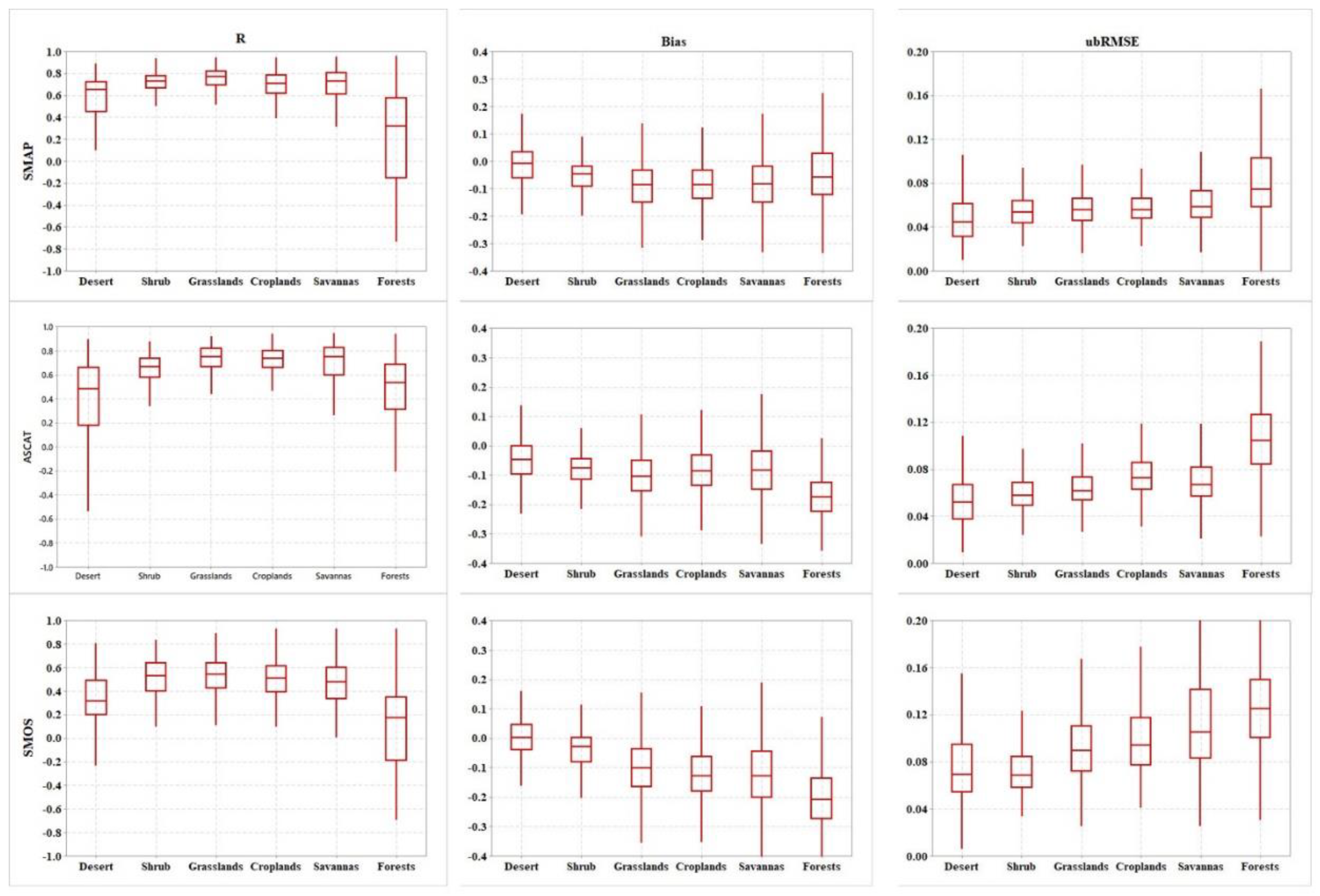
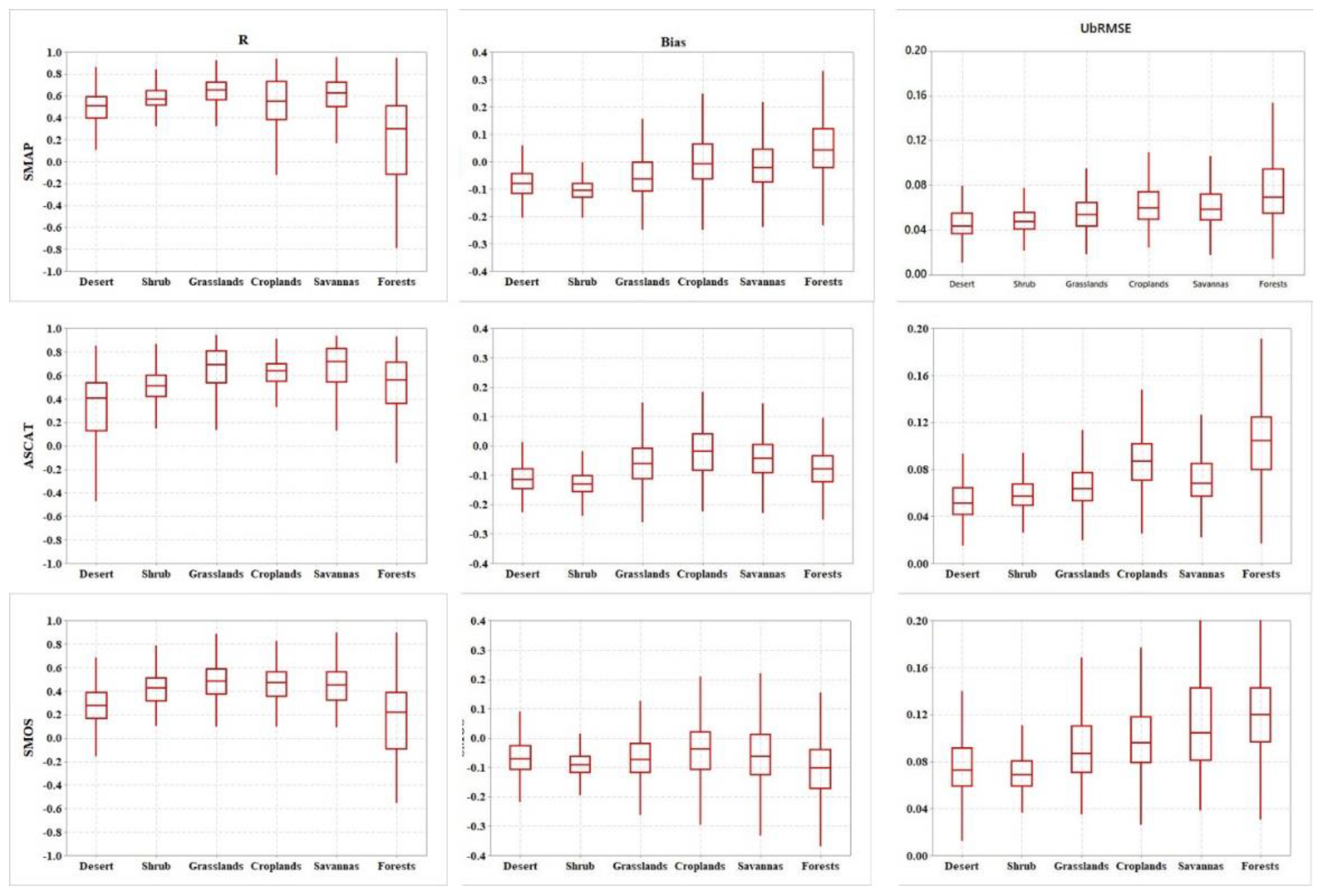
4.1. Assessment of Satellite SMO Products Against Reference Datasets

The results of comparing SMO products with the ERA5 and GLDAS in the SA from 14 May 2015 to 31 December 2016 are shown in Figure 5 and Figure 6, respectively. The insignificance estimates at a p-value of more than 0.05 between satellite SMO products and reference products were excluded. Because of the high level of RFI contamination, the SMOS displayed the largest excluded regions among the SMO products. Figure 7 and Figure 8 display the results of comparing satellites with ERA5 and GLDAS over various land surface covers of South America.

Over desert areas of dry climate zones as shown in Figure 1b, SMAP performs better than SMOS and ASCAT H113 (see Figure 7 and Figure 8), showing the highest correlations with both ERA5 and GLDAS, as well as the lowest bias and ubRMSE. These findings are consistent with studies such as the one by Chan et al. [54] that confirms SMAP’s sensitivity in arid, low-vegetation zones where microwave sensors more directly observe SMO. Meanwhile, ASCAT H113 showed moderate correlations and higher bias with both ERA5 and GLDAS. The reason for this is that the unexpected scattering volume from deeper soil layers or subsurface heterogeneity might lead active sensors to display a wet bias. These findings agree with prior studies, which identified that the backscatter amount was reduced in desert settings [31,55]. SMOS, showing the lowest correlation and highest ubRMSE, appears challenged in arid environments, where surface reflectivity can interfere with SMO retrieval accuracy [36].

In shrublands and grasslands, primarily located in areas with moderate average NDVI values and moderate rainfall amounts (see Figure 2 and Figure 3), SMAP continues to show strong performance by achieving the highest correlations, low bias, and low ubRMSE with both GLDAS and ERA5 (see Figure 7 and Figure 8). These regions have low-to-moderate vegetation density, allowing SMAP’s high-resolution microwave sensors to capture SMO accurately [56]. Meanwhile, ASCAT H113 also performs well in shrublands and grasslands, as shown in Figure 7 and Figure 8, with correlations close to SMAP’s, though its performance is slightly impacted by soil variability in transitional areas [57]. However, SMOS face challenges in these areas, with lower correlations and higher ubRMSE due to its coarser resolution and the presence of RFI. The coarser resolution of SMOS reduces its ability to capture fine-scale SMO variations accurately. This issue is clear in sparsely vegetated regions, as the decreasing vegetation cover increases the exposure to environmental noise and interference, further reducing data quality. Also, the presence of RFI can significantly affect the SMOS data quality, as excessive unauthorized emissions in the 1400–1427-Megahertz band can cause difficulties in accurate measurements [58,59,60].

In savannas and forest regions with high amounts of rainfall and high NDVI average value (see Figure 2 and Figure 3), specifically in the Amazon basin, all sensors face significant challenges due to dense canopy cover, which attenuates microwave signals and reduces accuracy. SMAP shows low average correlations and higher ubRMSE in forests with both GLDAS and ERA5 (see Figure 7 and Figure 8), in agreement with the results of Al-Yaari et al. [61] that indicate reduced performance in dense vegetation areas. ASCAT H113 performs slightly better in forested areas, showing moderate correlations with ERA5 and GLDAS. However, ASCAT H113 also displays higher bias and ubRMSE, reflecting challenges in dense vegetation due to the influence of vegetation dynamics on microwave backscatter, which complicates SM retrieval and affects the accuracy of the measurements [62,63,64]. SMOS exhibits the lowest correlations and highest ubRMSE in forested areas, as shown in Figure 7 and Figure 8, due to high opacity, which decreases radiometric sensitivity to observe SMO variations and complicates accurate retrieval [33,65]. These results indicate that SMAP is generally the most reliable product across most land cover types, while H113 and SMOS face limitations in forested areas with high biomass. The statistical results of comparing satellite SMO products with both GLDAS and ERA5 are listed in

Table 1. The overall average statistics of comparing satellite SMO products with reference datasets.

Overall Average Indexes	R		Bias		ubRMSE
	ERA5	GLDAS	ERA5	GLDAS	ERA5	GLDAS
SMAP	0.608	0.551	−0.014	−0.058	0.041	0.045
ASCAT	0.579	0.534	−0.064	−0.082	0.079	0.081
SMOS	0.439	0.380	−0.065	−0.093	0.109	0.111

. Regarding overall average statistics values, SMAP overall outperforms SMOS and ASCAT H113, with the highest average correlation (0.55 with GLDAS and 0.61 with ERA5), slight average bias (−0.058 with GLDAS and −0.014 with ERA5), and lowest average ubRMSE (0.045 with GLDAS and 0.041 with ERA5).

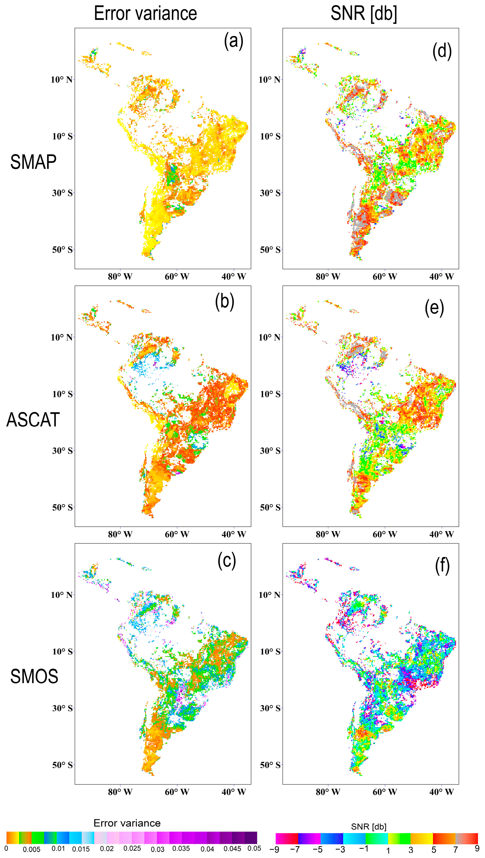
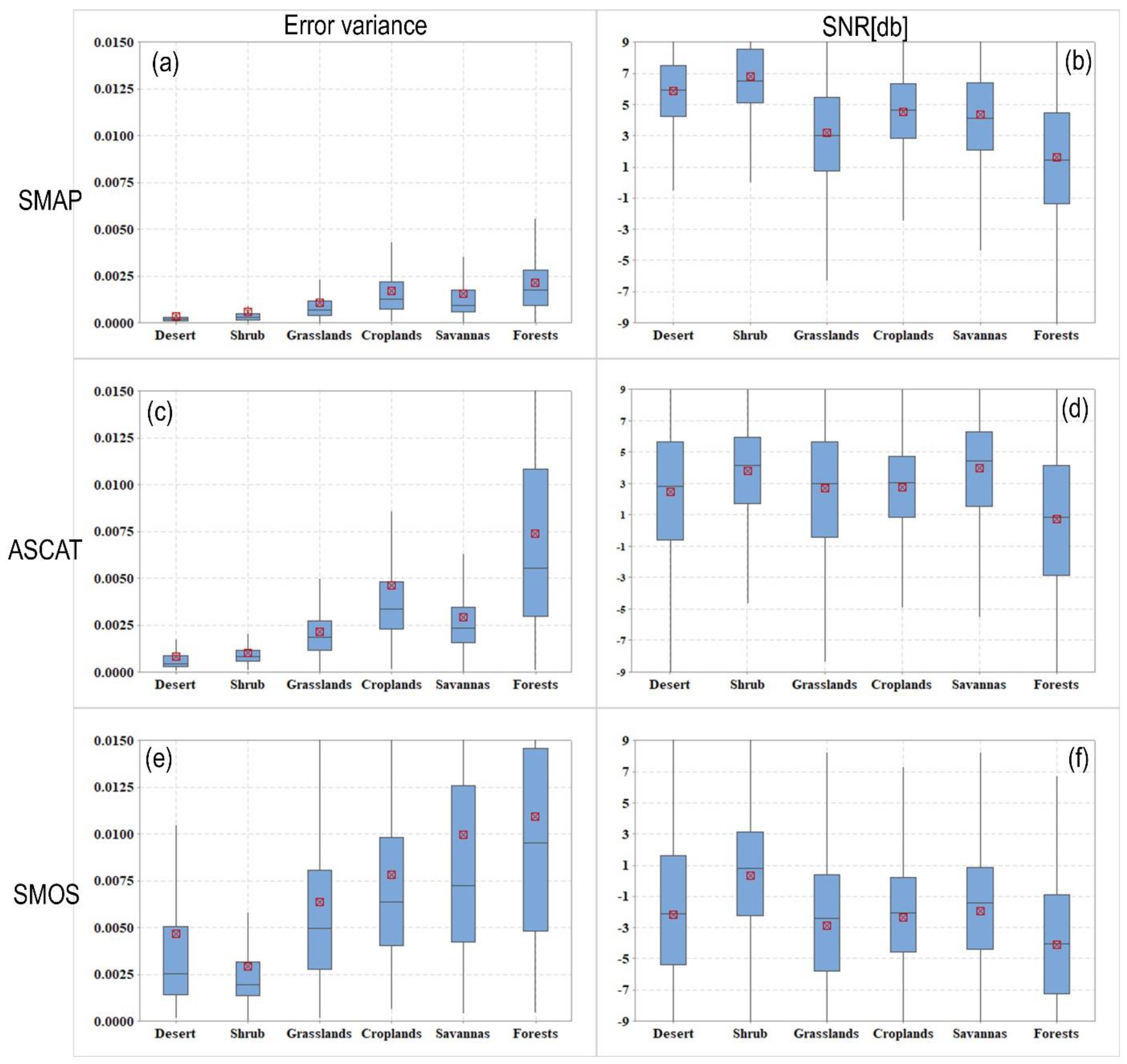
4.2. Triple Collocation Analysis

The results of S/N and the error variance for SMAP, SMOS, and ASCAT H113 SMO products are shown in Figure 9. These results are calculated for SMOS and ASCAT H113 from the first triplet (SMOS, ASCAT H113, and ERA5) and for SMAP from the second triplet (SMAP, ASCAT H113, and ERA5). The error variance values and (S/N) [dB] estimates of satellite SMO products across the land covers of SA are shown in Figure 10. The spatial agreement between the TCM results of ASCAT H113 and ERA5 with the two proposed triplets proves that TCM assumptions were considered. The results demonstrated that TCM metrics, which were computed using either GLDAS or ERA5 as the third dataset in the TCM triplet, have been consistent across the entirety of SA. Additionally, omitted areas are in one of the triplet products that did not contain measurements. These regions included the Amazonian tropical forests in the canter and nearly all the desert, especially in the southwestern parts of SA, where TCM cannot be used [66].

All satellites have low SMO variation in desert regions. Because the SMO signal changes were so little, they did not outweigh the instrument’s background noise. This makes using microwave-frequency measurements to retrieve SMO information more challenging. One of the difficulties in desert regions is associated with assessing the thickness of the emitting layer and the active temperature [67,68]. However, in the desert regions of SA within dry climate zones, as shown in Figure 1b, with extremely low rainfall amounts and a very low average NDVI value (see Figure 2 and Figure 3), SMAP demonstrated a marginally better performance in the desert than SMOS and H113 product of ASCAT, with a higher average (S/N) [dB] and a smaller average error variance.

In moderate vegetation regions, SMAP demonstrates robust performance, as evidenced by low error variance and high S/N in these areas (see Figure 10). These results are consistent with SMAP’s design to accurately retrieve SMO under moderate vegetation conditions, where microwave sensors face minimal interference from vegetation cover [48,61]. In contrast, in savannas and forest-dense regions, including the Amazon basin of tropical and temperate climate zones (see Figure 1a), SMAP shows slightly higher error variance and lower S/N, though it still outperforms ASCAT and SMOS. This is attributed to the dense canopy cover that attenuates SMAP’s microwave signals, reducing retrieval accuracy, a limitation commonly observed in forested areas for microwave-based SMO products [56].

As shown in Figure 9 and Figure 10c,d, The ASCAT H113 product shows moderate error variance values across the desert, shrubland, and grassland of South America, while showing higher error variance values in croplands and forested regions. This reflects that ASCAT has limitations in more dense vegetation lands, where vegetation and varying surface roughness can interfere with signal accuracy [55]. The surface dynamic with seasonal changes in vegetation cover within cropland can affect the backscatter signals from the ASCAT sensor, possibly leading to increased error [69,70]. The ASCAT H113 showed moderate S/N values (see Figure 9 and Figure 10) in shrublands, croplands, and grasslands. However, like SMAP, the ASCAT S/N decreased significantly in the Amazon basin of more dense vegetation. This error pattern agrees with the findings of [7,63,71]; they show that ASCAT, though effective in regions with less and moderate vegetation, encounters difficulties in dense vegetation areas due to volume scattering within the canopy. The decreased S/N in Amazon forest regions suggests that the ASCAT H113 product may not be as effective in SMO retrieving in these regions without additional calibration.

Across almost all land cover types of South America, as shown in Figure 9c and Figure 10e, The SMOS product shows the highest error variance among SMO products. These high errors are particularly in croplands, savannas, and forests, which may be attributed to SMOS’s L-band radiometer, which, while capable of penetrating moderate vegetation, struggles in more densely vegetated regions, where signals are more likely to be absorbed or scattered. In tropical regions, especially the Amazon basin, SMOS’s S/N is the lowest value, due to signal attenuation by canopy, surface scatter, and high vegetation water content, further complicating the accurate retrieval of SMO and other environmental parameters [65,72,73].

4.3. Spatiotemporal Variability and Interpretation

The results of Hovmöller diagrams for SMO datasets across SA are illustrated in Figure 11. These results prove that all products have the same average seasonal SMO dynamics in the SA. Nearest to the equator zone, clear seasonal variations are associated with the intertropical convergence zone and monsoon changes. The dynamic change in SMO from 14 May 2015 to 31 December 2015 is consistent with the same dates in 2016. SMO estimates are higher during the wet season (November–March), particularly in the Amazon rainforest and central Brazilian regions.

ERA5 and GLDAS (see Figure 11a,b) exhibit well-defined SMO gradients, with higher SMO levels, concentrated near the equator, especially during the wet season (November–March), and lower levels as latitude increases towards arid and semi-arid regions. This consistency in ERA5 and GLDAS, evident in clear seasonal patterns, reflects the advantages of these products as references for validation of SMO products across SA that combine atmospheric data with reliable modeling methods to capture seasonal variability more accurately [74,75,76]. However, ERA5 showed a better performance than GLDAS-Noah in representing SMO variability.

Also, all satellites showed an overall performance closer to ERA5’s than GLDAS-Noah’s. The SMAP product (see Figure 11c) shows a clear seasonal SMO variation, with more consistent SMO patterns across South America compared to SMOS and ASCAT (see Figure 11d,e). SMAP closely matches ERA5’s seasonal SMO variations, especially in regions with moderate vegetation (within 10°S to 30°S). This reveals that the passive SMAP is more sensitive to surface measures due to their depth of shallow sensing. The ASCAT H113 product captures general SMO seasonal variations with higher variability, indicating sensitivity to short-term weather events. However, the ASCAT H113 product shows noisier SMO signals, especially in regions above 20°S of more dense vegetation, including the Amazon basin, indicating the potential errors caused by vegetation or surface roughness interference [67]. The SMOS product captures certain SMO seasonal variations but exhibits significant noise, intensely in the nearest regions of the equator. SMOS exhibits slightly lower consistency with GLDAS and ERA5 datasets, especially in the Amazon regions (within 10°N to 10°S).

In this work, the results showed a relationship between rainfall and vegetation density across different land covers within the diverse climate zones of South America (see Figure 1, Figure 2 and Figure 3). This relationship emphasizes that the regional environmental characteristics within the diverse climate zones should be considered when choosing SMO products to guarantee accurate and reliable performance. The results of Hovmöller diagrams agree with our above analysis of comparing satellite datasets with reference SMO datasets and by applying TCM. SMAP and ASCAT showed relative robustness in arid and semi-arid to moderately vegetated areas compared to SMOS. The Amazon basin emerges as a critical region where all satellite SMO products displayed a significant SMO variability due to more dense vegetation cover. However, in the Amazon region, SMAP showed slightly better results than ASCAT H113 and SMOS. Thus, Hovmöller diagrams provided a comprehensive view of how these products capture seasonal SMO variations across SA diverse land covers and identify their anomalies and trends. SMAP provides smoother SMO estimates, ideal for regional climate studies. Based on the results, SMAP’s accurate SMO data can support drought forecasting, agricultural management, and hydrological research across South America [46].

Although SMAP performed better than ASCAT H113 and SMOS in tropical regions, none of the satellite SMO products offers highly reliable data, suggesting that alternative techniques or additional calibration may be essential for accurate monitoring in these regions. Our findings contribute to a nuanced understanding of satellite SMO product reliability over SA and offer practical guidance for their application in tropical and semi-arid ecosystems. In this study, we assessed the temporal agreement between satellite SMO products and GLDAS-Noah using absolute values. Although anomaly-based assessments can better isolate dynamic variability [77], our proposed approach used R and ubRMSE to mitigate systematic biases. Moreover, our comprehensive assessment, including validation against ERA5, triple collocation analysis, and Hovmöller diagrams, corroborated our findings when comparing satellite SMO products with GLDAS-Noah across diverse land covers in South America. Incorporating both absolute and anomaly-based methods is recommended for future studies to further enhance the robustness of satellite SMO assessments. The proposed approach provides a better understanding of satellite SMO products’ performance in regions with fewer or without ground stations.

5. Conclusions

In this study, we proposed an approach to assess the ASCAT H113, SMAP, and SMOS SMO retrievals across South America in the period from 14 May 2015 to 31 December 2016 based on the integration of some statistical methods. These methods include standard error metrics (R, bias, and ubRMSE), TCM, and Hovmöller diagrams. ERA5 and GLDAS-Noah SMO datasets were used as reference datasets for validation. The quality of SMO products was assessed by considering environmental variables within the different climate zones of SA. The results displayed that SMAP overall outperforms SMOS and ASCAT with the highest average correlation (0.55 with GLDAS and 0.61 with ERA5), slight average bias (−0.058 with GLDAS and −0.014 with ERA5), and lowest average ubRMSE (0.045 with GLDAS and 0.041 with ERA5). The triple collocation analysis is consistent with the results of comparing SMO products with ERA5 and GLDAS-Noah across different land covers of SA. In arid, semi-arid, and moderate vegetation regions, the SMAP satellite outperforms SMOS and ASCAT, achieving better statistics values with GLDAS and ERA5 datasets, and achieving low error variance and high S/N in the TCM analysis. While the ASCAT H113 product showed good performance, which makes it a good alternative to SMAP, it still has limitations in more dense vegetation regions. SMOS showed the lowest performance across SA, especially in the Amazon basin. SMAP products showed a clear seasonal SMO variation, with a more consistent SMO pattern across South America than SMOS and ASCAT. The Amazon basin emerges as a critical region where all SMO products displayed a significant SMO variability due to more dense vegetation cover; however, SMAP showed a slightly better performance than ASCAT and SMOS. The proposed approach provides a better understanding of satellite SMO products’ performance in regions with fewer or without ground truths. This research presents new spatiotemporal statistical insights into satellite SMO retrieval performance evaluation across diverse climate zones of SA. Also, it provides valuable guidance for improving SMO monitoring and agricultural management in semi-arid ecosystems and tropical land.

References

1. Wang, Y.; Shi, L.; Hu, Y.; Hu, X.; Song, W.; Wang, L. A comprehensive study of deep learning for soil moisture prediction. Hydrol. Earth Syst. Sci. 2024, 28, 917–943. [Google Scholar] [CrossRef]
2. Horton, D.; Johnson, J.T.; Al-Khaldi, M.; Baris, I.; Park, J.; Bindlish, R. Soil Moisture During 2015 Spring Flood Events from the SMAP Radar Time-Series Ratio Algorithm. In Proceedings of the 2024 United States National Committee of URSI National Radio Science Meeting, USNC-URSI NRSM 2024—Proceedings, Boulder, CO, USA, 9–12 January 2024; p. 352. [Google Scholar] [CrossRef]
3. Rajani, P.K.; Deshpande, G.; Goswami, M.; Kolhe, J.; Khandagale, V.; Mujumdar, M.; Singh, B.B. IoT-Based Low-Cost Soil Moisture and Soil Temperature Monitoring System. Int. J. Electr. Electron. Eng. 2023, 10, 66–74. [Google Scholar] [CrossRef]
4. Chaube, U.C.; Pandey, A.; Singh, V.P. Soil Moisture and Its Measurement. In Canal Irrigation Systems in India: Operation, Maintenance, and Management; Springer: Cham, Switzerland, 2023; pp. 471–483. [Google Scholar] [CrossRef]
5. Liu, Y.Y.; Parinussa, R.M.; Dorigo, W.A.; De Jeu, R.A.M.M.; Wagner, W.; van Dijk, A.I.J.M.; McCabe, M.F.; Evans, J.P. Developing an improved soil moisture dataset by blending passive and active microwave satellite-based retrievals. Hydrol. Earth Syst. Sci. 2011, 15, 425–436. [Google Scholar] [CrossRef]
6. Gao, Y.; Colliander, A.; Burgin, M.S.; Walker, J.P.; Chae, C.; Dinnat, E.; Cosh, M.H.; Caldwell, T.; Berg, A.; Martínez-Fernández, J. L-, C- and X-band passive microwave soil moisture retrieval algorithm parameterization using in situ validation sites. In Proceedings of the International Geoscience and Remote Sensing Symposium (IGARSS), Valencia, Spain, 22–27 July 2018; pp. 1434–1437. [Google Scholar] [CrossRef]
7. Wagner, W.; Lindorfer, R.; Hahn, S.; Kim, H.; Vreugdenhil, M.; Gruber, A.; Fischer, M.; Trnka, M. Global Scale Mapping of Subsurface Scattering Signals Impacting ASCAT Soil Moisture Retrievals. IEEE Trans. Geosci. Remote Sens. 2024, 62, 1–20. [Google Scholar] [CrossRef]
8. Mousa, B.G.; Shu, H.; Freeshah, M.; Tariq, A. A Novel Scheme for Merging Active and Passive Satellite Soil Moisture Retrievals Based on Maximizing the Signal to Noise Ratio. Remote Sens. 2020, 12, 3804. [Google Scholar] [CrossRef]
9. Gibon, F.; Mialon, A.; Richaume, P.; Rodríguez-Fernández, N.; Aberer, D.; Boresch, A.; Crapolicchio, R.; Dorigo, W.; Gruber, A.; Himmelbauer, I.; et al. Estimating the uncertainties of satellite derived soil moisture at global scale. Sci. Remote Sens. 2024, 10, 100147. [Google Scholar] [CrossRef]
10. Colliander, A.; Cosh, M.H.; Berg, A.; Misra, S.; Thomas, J.; Bourgeau-Chavez, L.; Kelly, V.; Kraatz, S.; Siqueira, P.; Roy, A.; et al. Development of SMAP Retrievals for Forested Regions: SMAPVEX19-22 and SMAPVEX22-Boreal. In Proceedings of the International Geoscience and Remote Sensing Symposium (IGARSS), Kuala Lumpur, Malaysia, 17–22 July 2022; pp. 4228–4231. [Google Scholar] [CrossRef]
11. Wang, P.; Zeng, J.; Chen, K.-S.; Ma, H.; Bi, H.; Chen, Q.; Letu, H. Effects of Spatial Heterogeneity on Satellite Soil Moisture Products. In Proceedings of theIGARSS 2024—2024 IEEE International Geoscience and Remote Sensing Symposium, Athens, Greece, 7–12 July 2024; pp. 5032–5035. [Google Scholar] [CrossRef]
12. Yang, W.; Guo, F.; Zhang, X.; Zhang, Z.; Zhu, Y. High temporal resolution quasi-global landscape soil freeze–thaw map from spaceborne GNSS-R technology and SMAP radiometer measurements. Int. J. Appl. Earth Obs. Geoinf. 2024, 128, 103777. [Google Scholar] [CrossRef]
13. Kim, H.; Parinussa, R.; Konings, A.G.; Wagner, W.; Cosh, M.H.; Lakshmi, V.; Zohaib, M.; Choi, M. Global-scale assessment and combination of SMAP with ASCAT (active) and AMSR2 (passive) soil moisture products. Remote Sens. Environ. 2018, 204, 260–275. [Google Scholar] [CrossRef]
14. Mousa, B.G.; Shu, H. Spatial Evaluation and Assimilation of SMAP, SMOS, and ASCAT Satellite Soil Moisture Products Over Africa Using Statistical Techniques. Earth Space Sci. 2020, 7, 1–16. [Google Scholar] [CrossRef]
15. Brocca, L.; Melone, F.; Moramarco, T.; Wagner, W.; Hasenauer, S. ASCAT soil wetness index validation through in situ and modeled soil moisture data in central Italy. Remote Sens. Environ. 2010, 114, 2745–2755. [Google Scholar] [CrossRef]
16. Gruber, A.; Dorigo, W.A.; Zwieback, S.; Xaver, A.; Wagner, W. Characterizing Coarse-Scale Representativeness of in situ Soil Moisture Measurements from the International Soil Moisture Network. Vadose Zone J. 2013, 12, 1–16. [Google Scholar] [CrossRef]
17. Dorigo, W.; Himmelbauer, I.; Aberer, D.; Schremmer, L.; Petrakovic, I.; Zappa, L.; Preimesberger, W.; Xaver, A.; Annor, F.; Ardö, J.; et al. The International Soil Moisture Network: Serving Earth system science for over a decade. Hydrol. Earth Syst. Sci. Discuss. 2021, 25, 1–83. [Google Scholar] [CrossRef]
18. Leroux, D.J.; Kerr, Y.H.; Al Bitar, A.; Bindlish, R.; Jackson, T.J.; Berthelot, B.; Portet, G.; Wagner, W.; Brocca, L.; Naeimi, V.; et al. Comparison Between SMOS, VUA, ASCAT, and ECMWF Soil Moisture Products Over Four Watersheds in U.S. IEEE Trans. Geosci. Remote Sens. 2014, 52, 1562–1571. [Google Scholar] [CrossRef]
19. Albergel, C.; de Rosnay, P.; Gruhier, C.; Muñoz-Sabater, J.; Hasenauer, S.; Isaksen, L.; Kerr, Y.; Wagner, W. Evaluation of remotely sensed and modelled soil moisture products using global ground-based in situ observations. Remote Sens. Environ. 2012, 118, 215–226. [Google Scholar] [CrossRef]
20. Su, C.-H.H.; Ryu, D.; Crow, W.T.; Western, A.W. Beyond triple collocation: Applications to soil moisture monitoring. J. Geophys. Res. 2014, 119, 6419–6439. [Google Scholar] [CrossRef]
21. Gruber, A.; Su, C.-H.; Zwieback, S.; Crow, W.; Dorigo, W.; Wagner, W. Recent advances in (soil moisture) triple collocation analysis. Int. J. Appl. Earth Obs. Geoinf. 2016, 45, 200–211. [Google Scholar] [CrossRef]
22. Persson, A. The Story of the Hovmöller Diagram: An (Almost) Eyewitness Account. Bull. Am. Meteorol. Soc. 2017, 98, 949–957. [Google Scholar] [CrossRef]
23. De-Leon, Y.; Paldor, N. Commonly used methods fail to detect known propagation speeds of simulated signals from time-longitude (Hovmöller) diagrams. Ocean Sci. 2019, 15, 1593–1599. [Google Scholar] [CrossRef]
24. Zaninelli, P.G.; Menéndez, C.G.; Falco, M.; López-Franca, N.; Carril, A.F. Future hydroclimatological changes in South America based on an ensemble of regional climate models. Clim. Dyn. 2019, 52, 819–830. [Google Scholar] [CrossRef]
25. Rossato, L.; de Jeu, R.; dos Santos Alvalá, R.C.; Souza, S. Evaluation of soil moisture from satellite observations over South America. Int. J. Remote Sens. 2011, 32, 8013–8031. [Google Scholar] [CrossRef]
26. Ma, H.; Zeng, J.; Chen, N.; Zhang, X.; Cosh, M.H.; Wang, W. Satellite surface soil moisture from SMAP, SMOS, AMSR2 and ESA CCI: A comprehensive assessment using global ground-based observations. Remote Sens. Environ. 2019, 231, 111215. [Google Scholar] [CrossRef]
27. Cui, C.; Xu, J.; Zeng, J.; Chen, K.-S.S.; Bai, X.; Lu, H.; Chen, Q.; Zhao, T. Soil Moisture Mapping from Satellites: An Intercomparison of SMAP, SMOS, FY3B, AMSR2, and ESA CCI over Two Dense Network Regions at Different Spatial Scales. Remote Sens. 2018, 10, 33. [Google Scholar] [CrossRef]
28. Zhang, X.; Zhang, T.; Zhou, P.; Shao, Y.; Gao, S.; Zhang, X.; Zhang, T.; Zhou, P.; Shao, Y.; Gao, S. Validation analysis of SMAP and AMSR2 soil moisture products over the United States using ground-based measurements. Remote Sens. 2017, 9, 104. [Google Scholar] [CrossRef]
29. Baker, J.C.A.; De Souza, D.C.; Kubota, P.Y.; Buermann, W.; Coelho, C.A.S.; Andrews, M.B.; Gloor, M.; Garcia-Carreras, L.; Figueroa, S.N.; Spracklen, D.V. An Assessment of Land–Atmosphere Interactions over South America Using Satellites, Reanalysis, and Two Global Climate Models. J. Hydrometeorol. 2021, 22, 905–922. [Google Scholar] [CrossRef]
30. Beck, H.E.; McVicar, T.R.; Vergopolan, N.; Berg, A.; Lutsko, N.J.; Dufour, A.; Zeng, Z.; Jiang, X.; van Dijk, A.I.J.M.; Miralles, D.G. High-resolution (1 km) Köppen-Geiger maps for 1901–2099 based on constrained CMIP6 projections. Sci. Data 2023, 10, 724. [Google Scholar] [CrossRef]
31. Colliander, A.; Jackson, T.J.J.; Bindlish, R.; Chan, S.; Das, N.; Kim, S.B.B.; Cosh, M.H.H.; Dunbar, R.S.S.; Dang, L.; Pashaian, L.; et al. Validation of SMAP surface soil moisture products with core validation sites. Remote Sens. Environ. 2017, 191, 215–231. [Google Scholar] [CrossRef]
32. Entekhabi, D.; Njoku, E.G.; O’Neill, P.E.; Kellogg, K.H.; Crow, W.T.; Edelstein, W.N.; Entin, J.K.; Goodman, S.D.; Jackson, T.J.; Johnson, J.; et al. The soil moisture active passive (SMAP) mission. Proc. IEEE 2010, 98, 704–716. [Google Scholar] [CrossRef]
33. Kerr, Y.H.; Waldteufel, P.; Richaume, P.; Wigneron, J.P.; Ferrazzoli, P.; Mahmoodi, A.; Al Bitar, A.; Cabot, F.; Gruhier, C.; Juglea, S.E.; et al. The SMOS soil moisture retrieval algorithm. IEEE Trans. Geosci. Remote Sens. 2012, 50, 1384–1403. [Google Scholar] [CrossRef]
34. Souza, A.G.S.S.; Neto, A.R.; Rossato, L.; Alvalá, R.C.S.; Souza, L.L. Use of SMOS L3 soil moisture data: Validation and drought assessment for Pernambuco State, Northeast Brazil. Remote Sens. 2018, 10, 1314. [Google Scholar] [CrossRef]
35. Parinussa, R.M.; Holmes, T.R.H.; Wanders, N.; Dorigo, W.A.; de Jeu, R.A.M.; Parinussa, R.M.; Holmes, T.R.H.; Wanders, N.; Dorigo, W.A.; Jeu, R.A.M. de A Preliminary Study toward Consistent Soil Moisture from AMSR2. J. Hydrometeorol. 2015, 16, 932–947. [Google Scholar] [CrossRef]
36. Al-Yaari, A.; Wigneron, J.P.; Dorigo, W.; Colliander, A.; Pellarin, T.; Hahn, S.; Mialon, A.; Richaume, P.; Fernandez-Moran, R.; Fan, L.; et al. Assessment and inter-comparison of recently developed/reprocessed microwave satellite soil moisture products using ISMN ground-based measurements. Remote Sens. Environ. 2019, 224, 289–303. [Google Scholar] [CrossRef]
37. Chen, F.; Crow, W.T.; Bindlish, R.; Colliander, A.; Burgin, M.S.; Asanuma, J.; Aida, K. Global-scale evaluation of SMAP, SMOS and ASCAT soil moisture products using triple collocation. Remote Sens. Environ. 2018, 214, 1–13. [Google Scholar] [CrossRef] [PubMed]
38. Wu, Z.; Feng, H.; He, H.; Zhou, J.; Zhang, Y. Evaluation of Soil Moisture Climatology and Anomaly Components Derived From ERA5-Land and GLDAS-2.1 in China. Water Resour. Manag. 2021, 35, 629–643. [Google Scholar] [CrossRef]
39. Hu, Z.; Chen, X.; Li, Y.; Zhou, Q.; Yin, G. Temporal and Spatial Variations of Soil Moisture Over Xinjiang Based on Multiple GLDAS Datasets. Front. Earth Sci. 2021, 9, 654848. [Google Scholar] [CrossRef]
40. Liu, Y.; Liu, Y.; Wang, W. Inter-comparison of satellite-retrieved and Global Land Data Assimilation System-simulated soil moisture datasets for global drought analysis. Remote Sens. Environ. 2019, 220, 1–18. [Google Scholar] [CrossRef]
41. Li, N.; Zhou, C.; Zhao, P. The Validation of Soil Moisture from Various Sources and Its Influence Factors in the Tibetan Plateau. Remote Sens. 2022, 14, 4109. [Google Scholar] [CrossRef]
42. Araki, R.; Mu, Y.; McMillan, H. Evaluation of GLDAS soil moisture seasonality in arid climates. Hydrol. Sci. J. 2023, 68, 1109–1126. [Google Scholar] [CrossRef]
43. Zhuang, R.; Zeng, Y.; Manfreda, S.; Su, Z. Quantifying long-term land surface and root zone soil moisture over Tibetan plateau. Remote Sens. 2020, 12, 509. [Google Scholar] [CrossRef]
44. Beck, H.E.; Pan, M.; Miralles, D.G.; Reichle, R.H.; Dorigo, W.A.; Hahn, S.; Sheffield, J.; Karthikeyan, L.; Balsamo, G.; Parinussa, R.M.; et al. Evaluation of 18 satellite- and model-based soil moisture products using in situ measurements from 826 sensors. Hydrol. Earth Syst. Sci. Discuss. 2020, 25, 17–40. [Google Scholar] [CrossRef]
45. Albergel, C.; Munier, S.; Calvet, J.; Dutra, E.; Munoz-Sabater, J.; DeRosnay, P.; Balsamo, G. ERA-5 and ERA-Interim driven ISBA land surface model simulations: Which one performs better? Hydrol. Earth Syst. Sci. 2018, 22, 3515–3532. [Google Scholar] [CrossRef]
46. Friedl, M.A.; Sulla-Menashe, D.; Schneider, A.; Ramankutty, N.; Sibley, A.; Huang, X. MODIS Collection 5 global land cover: Algorithm refinements and characterization of new datasets. Remote Sens. Environ. 2010, 114, 168–182. [Google Scholar] [CrossRef]
47. Schneider, U.; Becker, A.; Finger, P.; Meyer-Christoffer, A.; Ziese, M. GPCC Full Data Monthly Version 2018.0 at 0.25°: Monthly Land-Surface Precipitation from Rain-Gauges Built on GTS-Based and Historic Data; GPCC at Deutscher Wetterdienst: Offenbach, Germany, 2018. [Google Scholar] [CrossRef]
48. Chan, S.K.; Bindlish, R.; O’Neill, P.; Jackson, T.; Njoku, E.; Dunbar, S.; Chaubell, J.; Piepmeier, J.; Yueh, S.; Entekhabi, D.; et al. Development and assessment of the SMAP enhanced passive soil moisture product. Remote Sens. Environ. 2018, 204, 931–941. [Google Scholar] [CrossRef] [PubMed]
49. Paulik, C.; Dorigo, W.; Wagner, W.; Kidd, R. Validation of the ASCAT Soil Water Index using in situ data from the International Soil Moisture Network. Int. J. Appl. Earth Obs. Geoinf. 2014, 30, 1–8. [Google Scholar] [CrossRef]
50. Wang, P.; Zeng, J.; Chen, K.S.; Ma, H.; Zhang, X.; Shi, P.; Peng, C.; Bi, H. Global-Scale Assessment of Multiple Recently Developed/Reprocessed Remotely Sensed Soil Moisture Datasets. IEEE Trans. Geosci. Remote Sens. 2024, 62, 1–18. [Google Scholar] [CrossRef]
51. Entekhabi, D.; Reichle, R.H.; Koster, R.D.; Crow, W.T.; Entekhabi, D.; Reichle, R.H.; Koster, R.D.; Crow, W.T. Performance Metrics for Soil Moisture Retrievals and Application Requirements. J. Hydrometeorol. 2010, 11, 832–840. [Google Scholar] [CrossRef]
52. McColl, K.A.; Vogelzang, J.; Konings, A.G.; Entekhabi, D.; Piles, M.; Stoffelen, A. Extended triple collocation: Estimating errors and correlation coefficients with respect to an unknown target. Geophys. Res. Lett. 2014, 41, 6229–6236. [Google Scholar] [CrossRef]
53. Hocke, K.; Kämpfer, N. Hovmöller diagrams of climate anomalies in NCEP/NCAR reanalysis from 1948 to 2009. Clim. Dyn. 2011, 36, 355–364. [Google Scholar] [CrossRef]
54. Li, C.; Tang, G.; Hong, Y. Cross-evaluation of ground-based, multi-satellite and reanalysis precipitation products: Applicability of the Triple Collocation method across Mainland China. J. Hydrol. 2018, 562, 71–83. [Google Scholar] [CrossRef]
55. Wagner, W.; Hahn, S.; Kidd, R.; Melzer, T.; Bartalis, Z.; Hasenauer, S.; Figa-Saldaña, J.; De Rosnay, P.; Jann, A.; Schneider, S.; et al. The ASCAT soil moisture product: A review of its specifications, validation results, and emerging applications. Meteorol. Z. 2013, 22, 5–33. [Google Scholar] [CrossRef]
56. Chen, Q.; Zeng, J.; Cui, C.; Li, Z.; Chen, K.S.; Bai, X.; Xu, J. Soil Moisture Retrieval from SMAP: A Validation and Error Analysis Study Using Ground-Based Observations over the Little Washita Watershed. IEEE Trans. Geosci. Remote Sens. 2018, 56, 1398–1408. [Google Scholar] [CrossRef]
57. Brocca, L.; Hasenauer, S.; Lacava, T.; Melone, F.; Moramarco, T.; Wagner, W.; Dorigo, W.; Matgen, P.; Martínez-Fernández, J.; Llorens, P.; et al. Soil moisture estimation through ASCAT and AMSR-E sensors: An intercomparison and validation study across Europe. Remote Sens. Environ. 2011, 115, 3390–3408. [Google Scholar] [CrossRef]
58. Pablos, M.; Turiel, A.; Camps, A.; Vall-Llossera, M.; Portabella, M.; González-Haro, C.; Olmedo, E.; López-Martínez, C. Spatial Spectra Assessment of SMOS Soil Moisture at Different Spatial Scales. In Proceedings of the IGARSS 2024—2024 IEEE International Geoscience and Remote Sensing Symposium, Athens, Greece, 7–12 July 2024; pp. 5147–5150. [Google Scholar] [CrossRef]
59. Xu, M.; Li, H.; Chen, H.; Yin, X. Quantitative Measurement of Radio Frequency Interference for SMOS Mission. Remote Sens. 2022, 14, 1669. [Google Scholar] [CrossRef]
60. Uranga, E.; Llorente, Á.; González, J.; de la Fuente, A.; Oliva, R.; Soldo, Y.; Jorge, F. SMOS ESA RFI Monitoring and Information Tool: Lessons Learned. Remote Sens. 2022, 14, 5387. [Google Scholar] [CrossRef]
61. Al-Yaari, A.; Wigneron, J.-P.P.; Kerr, Y.; Rodriguez-Fernandez, N.; O’Neill, P.E.E.; Jackson, T.J.J.; De Lannoy, G.J.M.J.M.; Al Bitar, A.; Mialon, A.; Richaume, P.; et al. Evaluating soil moisture retrievals from ESA’s SMOS and NASA’s SMAP brightness temperature datasets. Remote Sens. Environ. 2017, 193, 257–273. [Google Scholar] [CrossRef]
62. Ma, H.; Zeng, J.; Zhang, X.; Peng, J.; Li, X.; Fu, P.; Cosh, M.H.; Letu, H.; Wang, S.; Chen, N.; et al. Surface soil moisture from combined active and passive microwave observations: Integrating ASCAT and SMAP observations based on machine learning approaches. Remote Sens. Environ. 2024, 308, 114197. [Google Scholar] [CrossRef]
63. Vreugdenhil, M.; Dorigo, W.A.; Wagner, W.; De Jeu, R.A.M.; Hahn, S.; Van Marle, M.J.E. Analyzing the Vegetation Parameterization in the TU-Wien ASCAT Soil Moisture Retrieval. IEEE Trans. Geosci. Remote Sens. 2016, 54, 3513–3531. [Google Scholar] [CrossRef]
64. Greimeister-Pfeil, I.; Wagner, W.; Quast, R.; Hahn, S.; Steele-Dunne, S.; Vreugdenhil, M. Disentangling soil moisture and vegetation effects on the ASCAT backscatter-incidence angle relationship. In EGU General Assembly Conference Abstracts EGU22-5128, Proceedings of the EGU General Assembly, Vienna, Austria, 23–27 May 2022; European Geosciences Union: Vienna, Austria, 2022. [Google Scholar] [CrossRef]
65. Vittucci, C.; Ferrazzoli, P.; Kerr, Y.H.; Richaume, P.; Laurin, G.V.; Guerriero, L. Analysis of Vegetation Optical Depth and Soil Moisture Retrieved by SMOS over Tropical Forests. IEEE Geosci. Remote Sens. Lett. 2019, 16, 504–508. [Google Scholar] [CrossRef]
66. Scipal, K.; Holmes, T.; De Jeu, R.; Naeimi, V.; Wagner, W. A possible solution for the problem of estimating the error structure of global soil moisture data sets. Geophys. Res. Lett. 2008, 35, 2–5. [Google Scholar] [CrossRef]
67. Dorigo, W.A.; Scipal, K.; Parinussa, R.M.; Liu, Y.Y.; Wagner, W.; de Jeu, R.A.M.M.; Naeimi, V. Error characterisation of global active and passive microwave soil moisture datasets. Hydrol. Earth Syst. Sci. 2010, 14, 2605–2616. [Google Scholar] [CrossRef]
68. Holmes, T.R.H.; de Rosnay, P.; de Jeu, R.; Wigneron, R.J.-P.; Kerr, Y.; Calvet, J.-C.; Escorihuela, M.J.; Saleh, K.; Lemaître, F. A new parameterization of the effective temperature for L band radiometry. Geophys. Res. Lett. 2006, 33, L07405. [Google Scholar] [CrossRef]
69. Steele-Dunne, S.C.; Hahn, S.; Wagner, W.; Vreugdenhil, M. Towards Including Dynamic Vegetation Parameters in the EUMETSAT H SAF ASCAT Soil Moisture Products. Remote Sens. 2021, 13, 1463. [Google Scholar] [CrossRef]
70. Albergel, C.; Rüdiger, C.; Carrer, D.; Calvet, J.-C.C.; Fritz, N.; Naeimi, V.; Bartalis, Z.; Hasenauer, S. An evaluation of ASCAT surface soil moisture products with in-situ observations in Southwestern France. Hydrol. Earth Syst. Sci. 2009, 13, 115–124. [Google Scholar] [CrossRef]
71. Petchiappan, A.; Steele-Dunne, S.C.; Vreugdenhil, M.; Hahn, S.; Wagner, W.; Oliveira, R. The influence of vegetation water dynamics on the ASCAT backscatter-incidence angle relationship in the Amazon. Hydrol. Earth Syst. Sci. 2022, 26, 2997–3019. [Google Scholar] [CrossRef]
72. Kerr, Y.H.; Al-Yaari, A.; Rodriguez-Fernandez, N.; Parrens, M.; Molero, B.; Leroux, D.; Bircher, S.; Mahmoodi, A.; Mialon, A.; Richaume, P.; et al. Overview of SMOS performance in terms of global soil moisture monitoring after six years in operation. Remote Sens. Environ. 2016, 180, 40–63. [Google Scholar] [CrossRef]
73. Parrens, M.; Al Bitar, A.; Frappart, F.; Papa, F.; Calmant, S.; Crétaux, J.F.; Wigneron, J.P.; Kerr, Y. Mapping Dynamic Water Fraction under the Tropical Rain Forests of the Amazonian Basin from SMOS Brightness Temperatures. Water 2017, 9, 350. [Google Scholar] [CrossRef]
74. Yang, S.; Li, R.; Wu, T.; Hu, G.; Xiao, Y.; Du, Y.; Zhu, X.; Ni, J.; Ma, J.; Zhang, Y.; et al. Evaluation of reanalysis soil temperature and soil moisture products in permafrost regions on the Qinghai-Tibetan Plateau Shuhua. Geoderma 2020, 377, 114583. [Google Scholar] [CrossRef]
75. Hersbach, H.; Bell, B.; Berrisford, P.; Hirahara, S.; Horányi, A.; Muñoz-Sabater, J.; Nicolas, J.; Peubey, C.; Radu, R.; Schepers, D.; et al. The ERA5 global reanalysis. Q. J. R. Meteorol. Soc. 2020, 146, 1999–2049. [Google Scholar] [CrossRef]
76. Rodell, M.; Houser, P.R.; Jambor, U.; Gottschalck, J.; Mitchell, K.; Meng, C.J.; Arsenault, K.; Cosgrove, B.; Radakovich, J.; Bosilovich, M.; et al. The Global Land Data Assimilation System. Bull. Am. Meteorol. Soc. 2004, 85, 381–394. [Google Scholar] [CrossRef]
77. Spennemann, P.C.; Rivera, J.A.; Celeste Saulo, A.; Penalba, O.C. A comparison of GLDAS soil moisture anomalies against standardized precipitation index and multisatellite estimations over South America. J. Hydrometeorol. 2015, 16, 158–171. [Google Scholar] [CrossRef]
Figure 1. (a) Köppen–Geiger climate classification map for South America. Where the different climate zones are tropical (Af, Am, and Aw), dry (BWk, BWh, BSk, and BSh), temperate (Cfa, Cfb, Cfc, Csa, Csb, Csc, Cwa, Cwb, and Cwc), and polar (ET). (b) The land cover classification across SA. Observe that there are fewer available ground SMO stations in SA hosted by ISMN, and they are denoted by red on the map.
Remotesensing 17 00753 g001
Figure 2. (a) Spatial distribution of average NDVI values. (b) The distribution of rainfall amounts across SA.
Remotesensing 17 00753 g002
Figure 3. The correlation between NDVI and rainfall across land cover types in SA. Note that the values in this chart represent NDVI average values and rainfall amounts in the unit of mm/study period.
Remotesensing 17 00753 g003
Figure 4. The proposed approach to investigate the performance of satellite SMO products in SA.
Remotesensing 17 00753 g004
Figure 5. The results of comparing satellite datasets with ERA5 across SA for the SMAP (1st column), ASCAT H113 (2nd column), and SMOS (3rd): (ac) for R results, bias results (df), and ubRMSE results (gi). The excluded results are represented by white regions on the maps.
Remotesensing 17 00753 g005
Figure 6. The results of comparing satellite datasets with GLDAS across SA for the SMAP (1st column), ASCAT H113 (2nd column), and SMOS (3rd): (ac) for R results, bias results (df), and ubRMSE results (gi). The excluded results are represented by white areas on the maps.
Remotesensing 17 00753 g006
Figure 7. The results of comparing SMO datasets with the ERA5 dataset across different land surface covers. SMAP (1st row), ASCAT H113 (2nd row), and SMOS (3rd row): the 1st column for R values, the 2nd column for results of bias, and the 3rd column for ubRMSE values.
Remotesensing 17 00753 g007
Figure 8. The results of comparing SMO datasets with the GLDAS dataset across different land surface covers. SMAP (1st row), ASCAT H113 (2nd row), and SMOS (3rd row): the 1st column for R values, the 2nd column for results of bias, and the 3rd column for ubRMSE values.
Remotesensing 17 00753 g008
Figure 9. The TCM analysis for satellite SMO datasets in SA, where the SMAP (1st row), ASCAT H113 (2nd row), and SMOS (3rd row): error variance (ac), (S/N) [db] (df). The excluded results are represented by white regions on the maps.
Remotesensing 17 00753 g009
Figure 10. The error variance values and (S/N) [dB] estimates of satellite SMO products across the land covers of SA for SMAP (1st row), ASCAT H113 (2nd row), and SMOS (3rd row): error variance (a,c,e), (S/N) [db] (b,d,f). The mean values represented with red symbol.
Remotesensing 17 00753 g010
Figure 11. The spatiotemporal variability of SMO products across SA from 14 May 2015 to 31 December 2016, including (a) ERA5, (b) GLDAS, (c) SMAP, (d) ASCAT H113, and (e) SMOS.
Remotesensing 17 00753 g011