

Quantitative Remote Sensing Supporting Deep Learning Target Identification: A Case Study of Wind Turbines

 ,
,  ,
,
Abstract

1. Introduction
- (1)
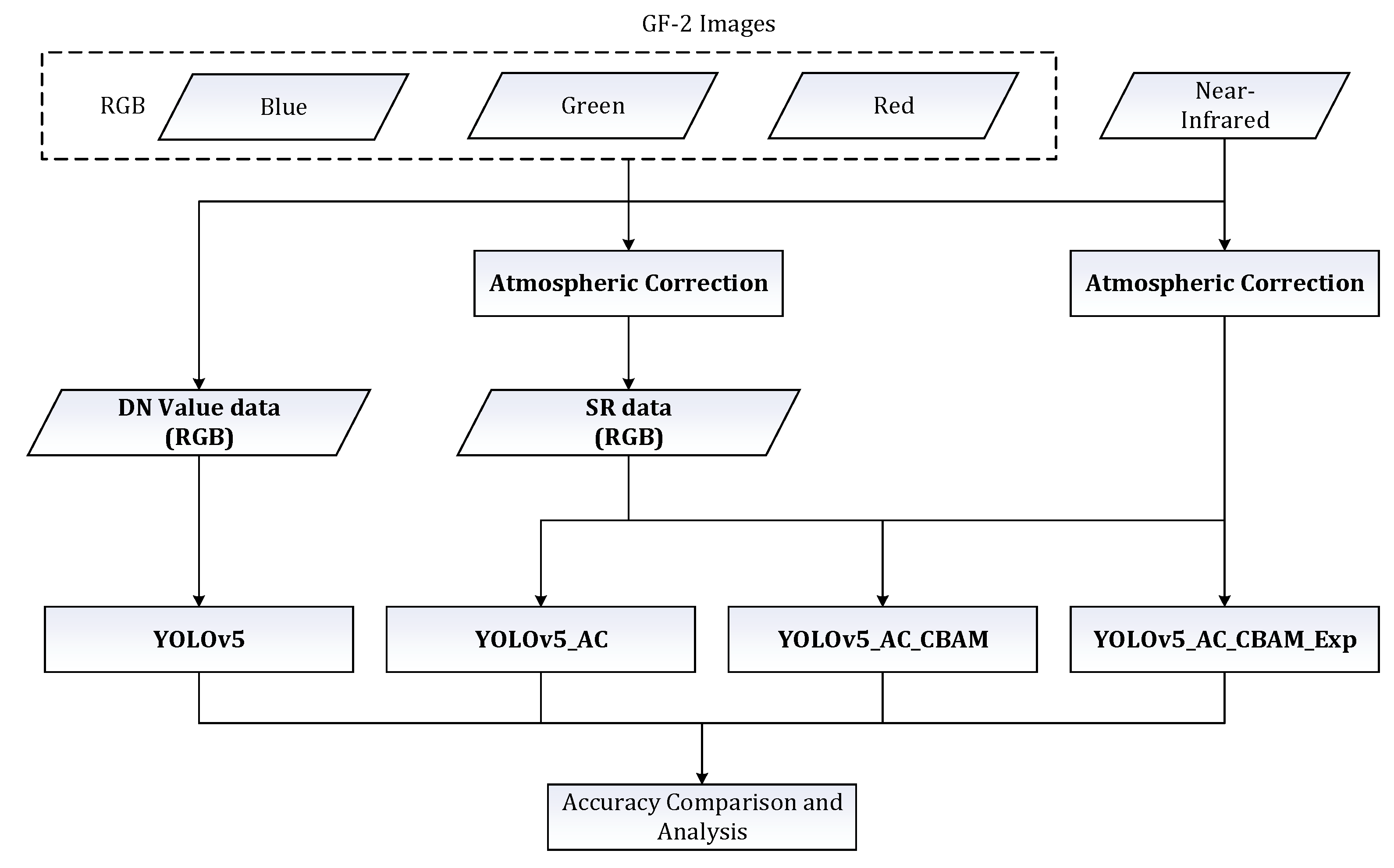
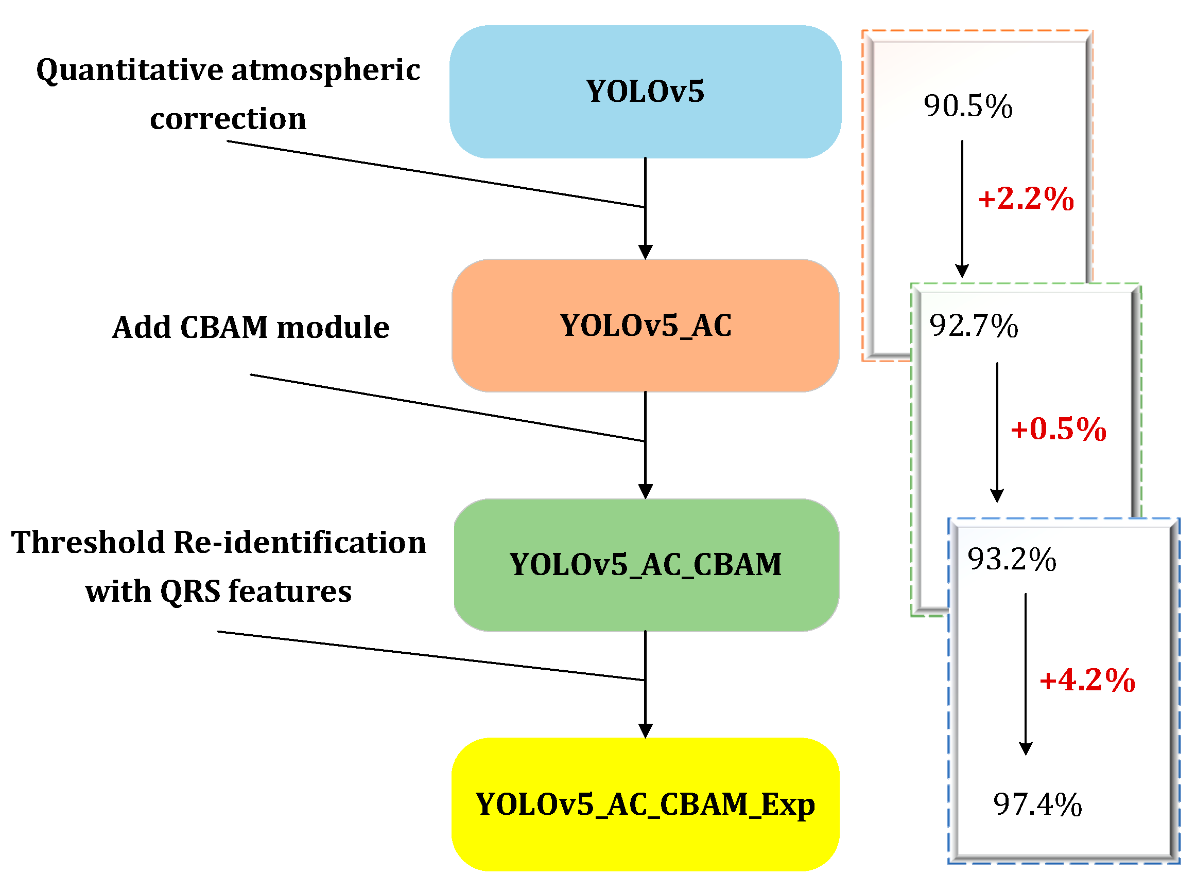
- Quantitative AC processing was incorporated into the preprocessing stage of HSR images to restore the true spectral characteristics of ground objects. Two distinct types of HSR wind turbine sample databases were established. One was the DN (Digital Number) value sample database, which lacks RS features due to the absence of quantitative AC in the image preprocessing stage. The other was the SR sample database, which preserves spectral reflectance and other RS features as a result of the inclusion of quantitative AC during preprocessing. Compared with DN value data, the performance of SR data was significantly enhanced for TDI on the YOLOv5 model.
- (2)
- The Convolutional Block Attention Module (CBAM) attention mechanism was introduced into the neck part of the YOLOv5 model to enhance the effective feature information of the wind turbine target, and the model identification effect was improved to some extent.
- (3)
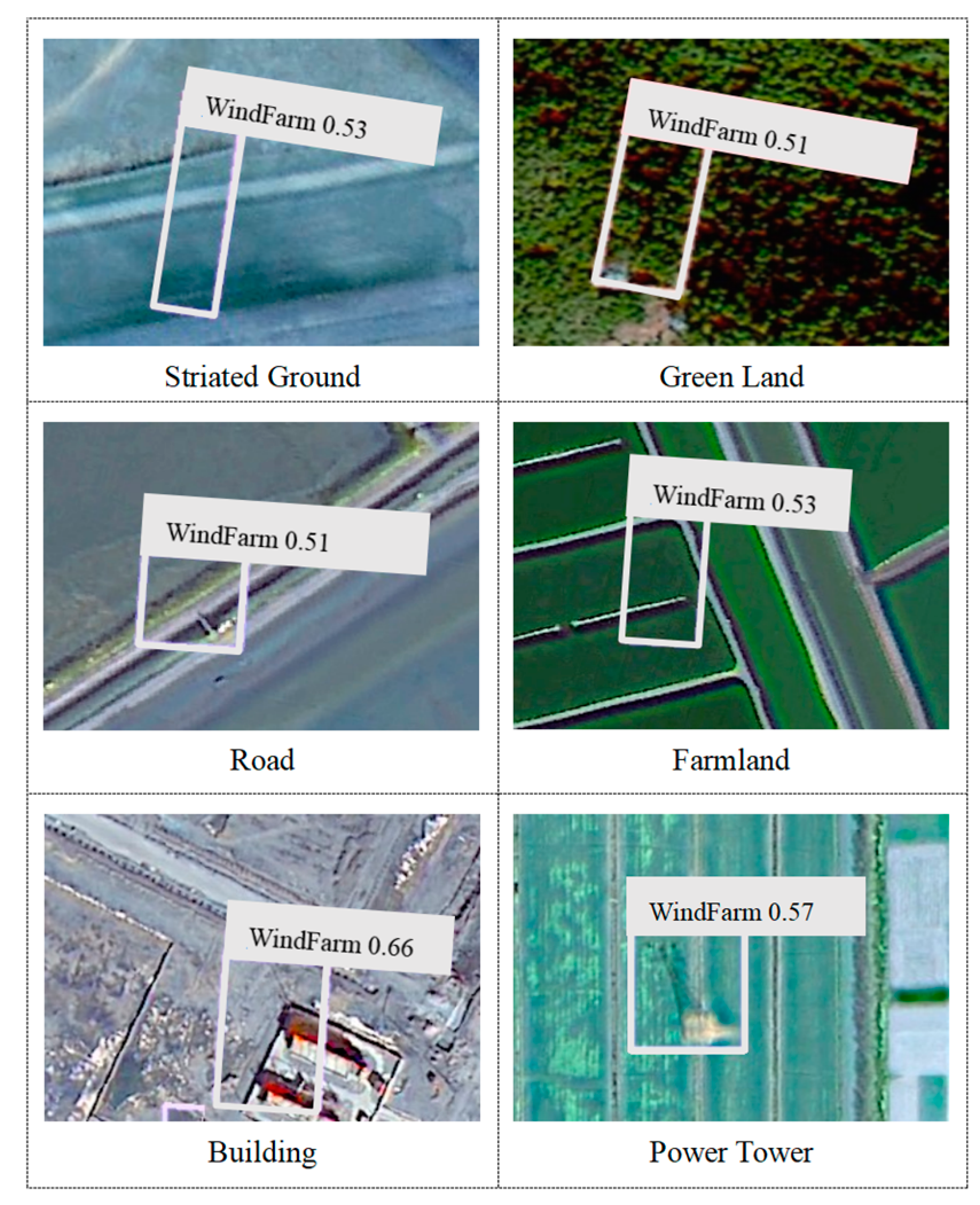
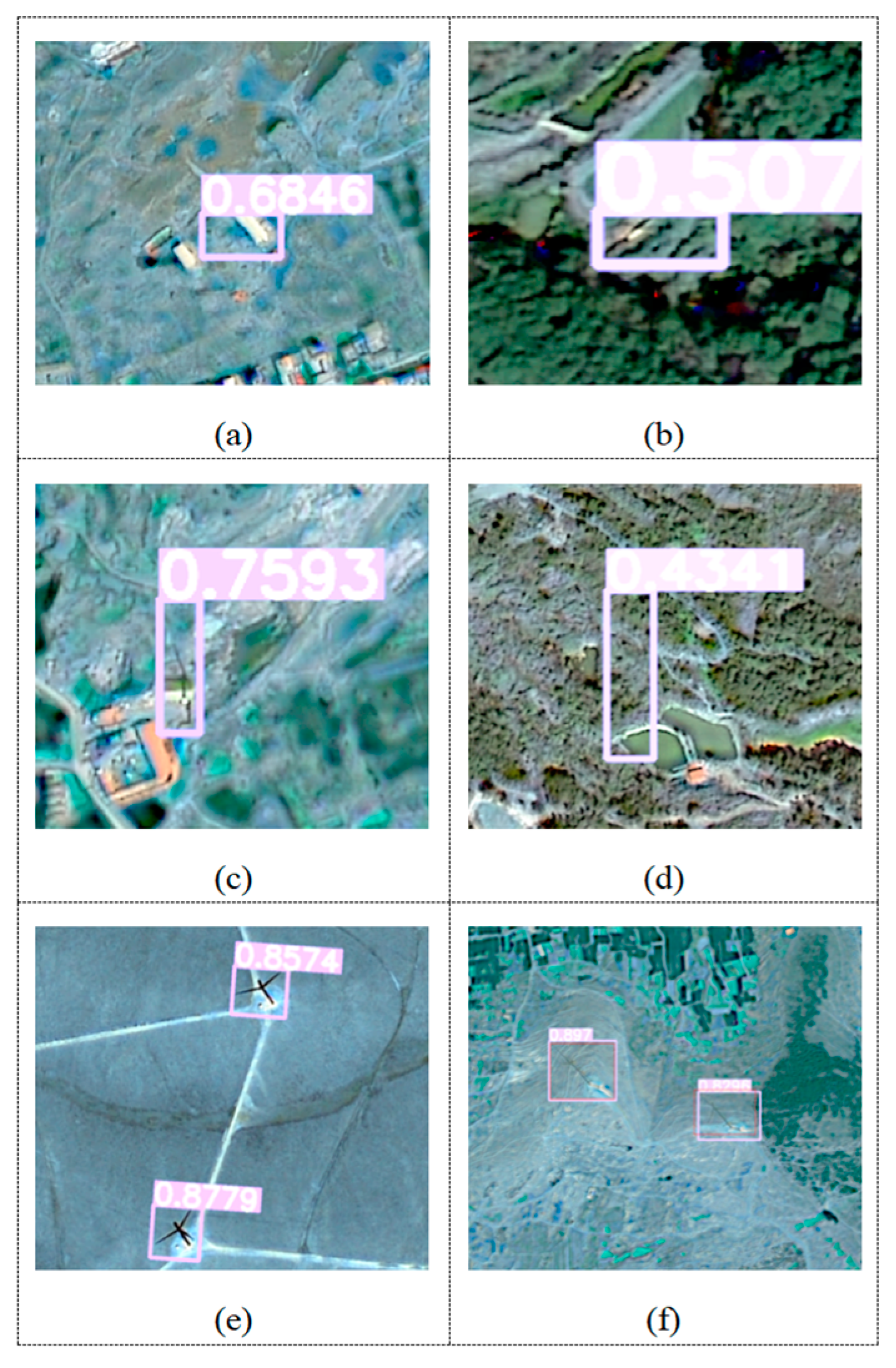
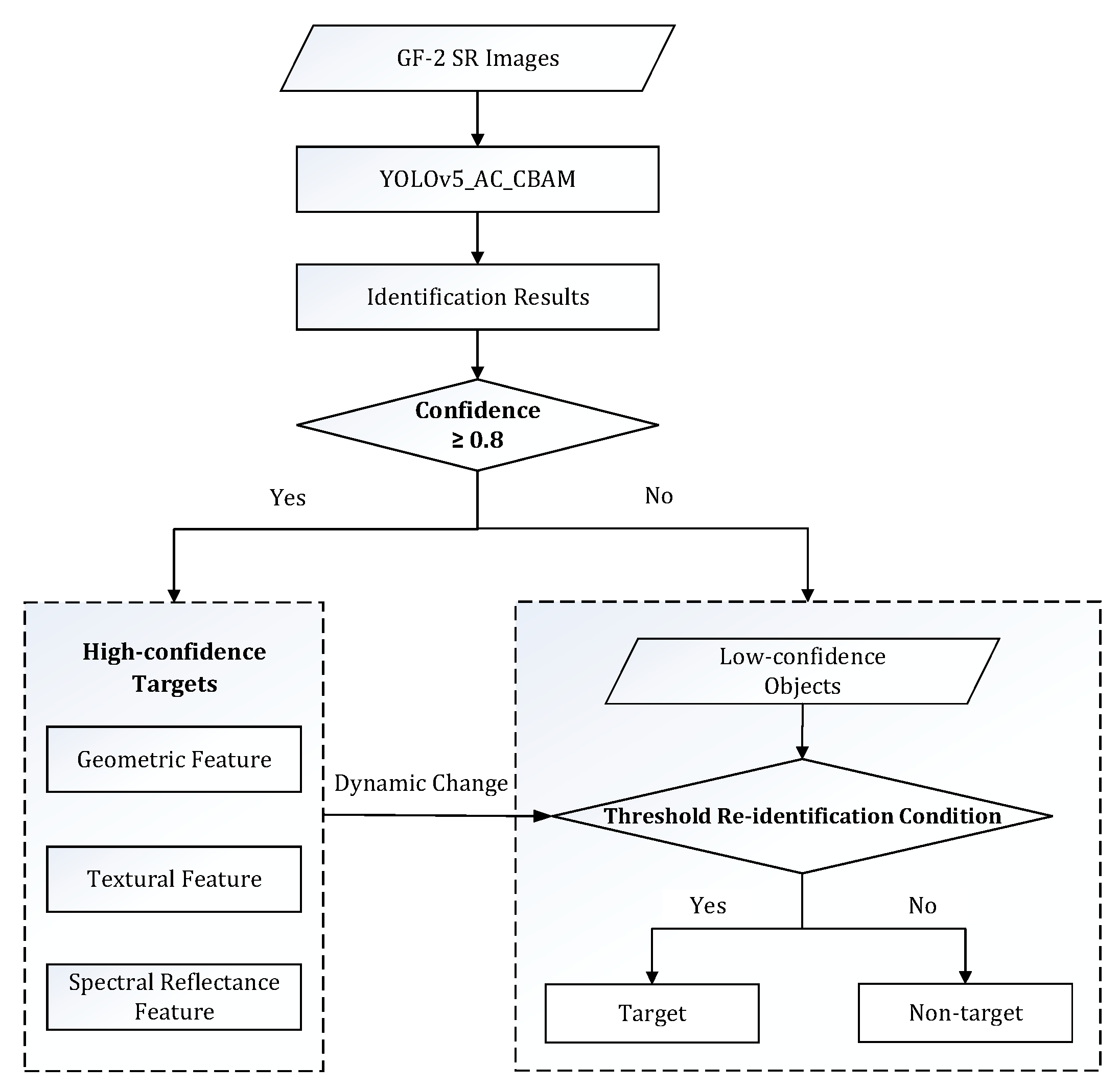
- Based on the identification results of the model, the unique quantitative spectral reflectance, geometry, and texture features of the wind turbine target were selected using RS expert knowledge as the dynamic threshold discrimination conditions, and the re-identification of the wind turbine was further carried out. The integration of quantitative information effectively eliminated many false detection objects, and the performance was excellent.
2. Related Work
2.1. Optical RS Image TDI
2.2. Hyperspectral Image Classification and Identification
3. Materials and Methods
3.1. GF-2 Satellite Images and Wind Turbine Sample Databases
3.1.1. GF-2 Satellite Images
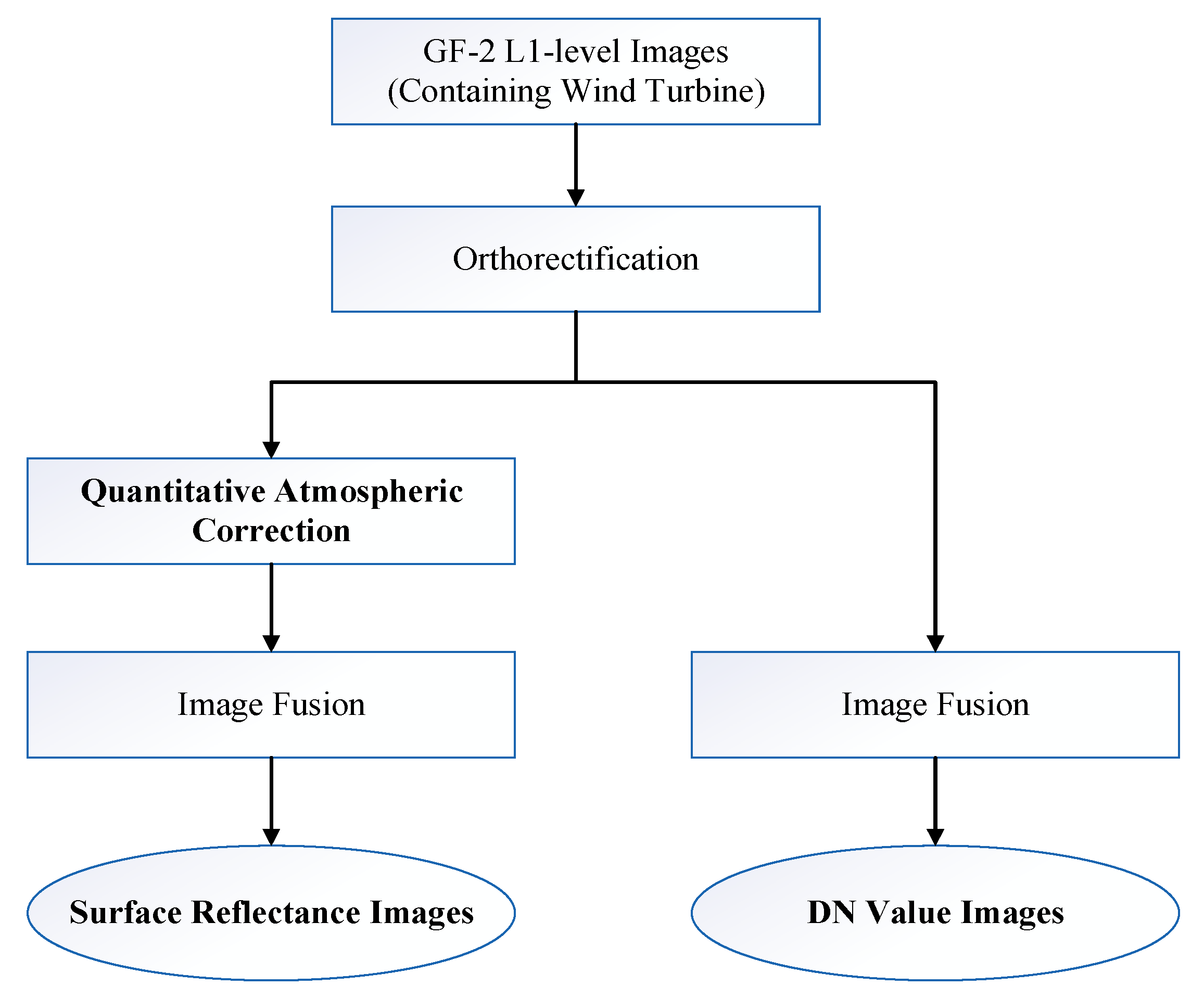
3.1.2. Data Preprocessing
3.1.3. Sample Labeling
3.2. Experimental Strategy and Methods
3.2.1. YOLOv5
3.2.2. YOLOv5_AC
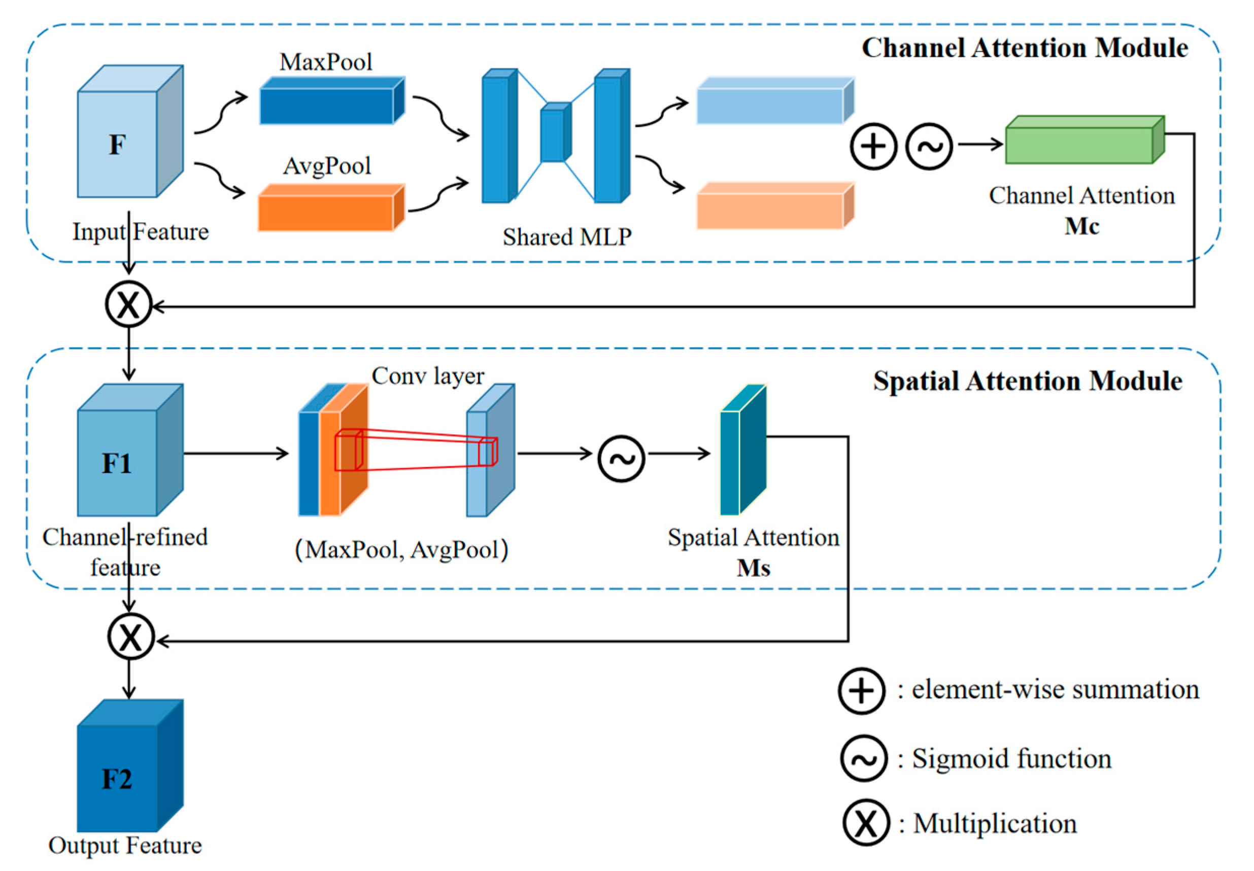
3.2.3. YOLOv5_AC_CBAM
3.2.4. YOLOv5_AC_CBAM_Exp
- (1)
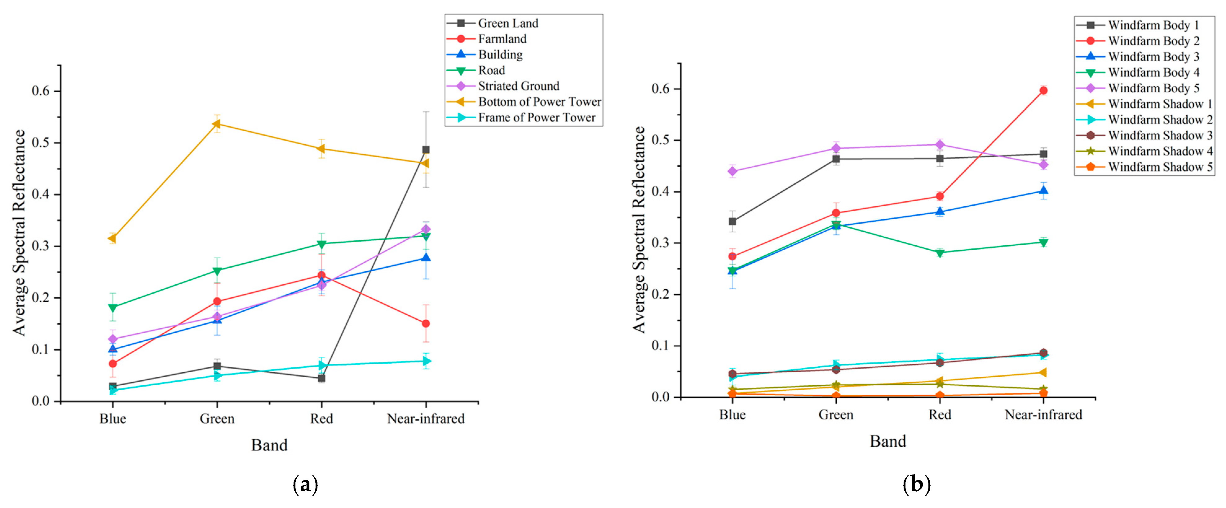
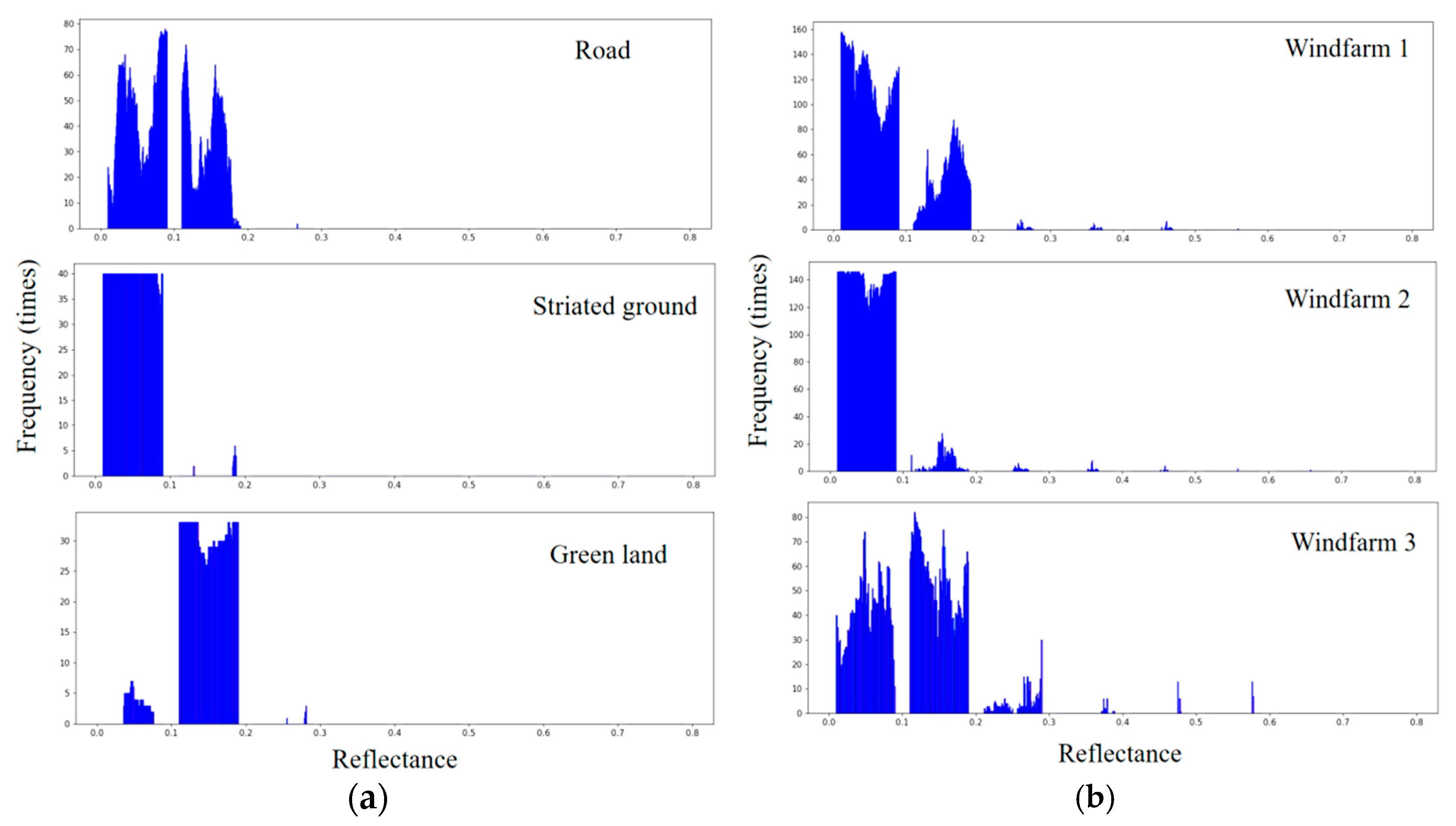
- Quantitative Spectral Reflectance Feature Selection
- (2)
- Quantitative Geometric Feature Selection
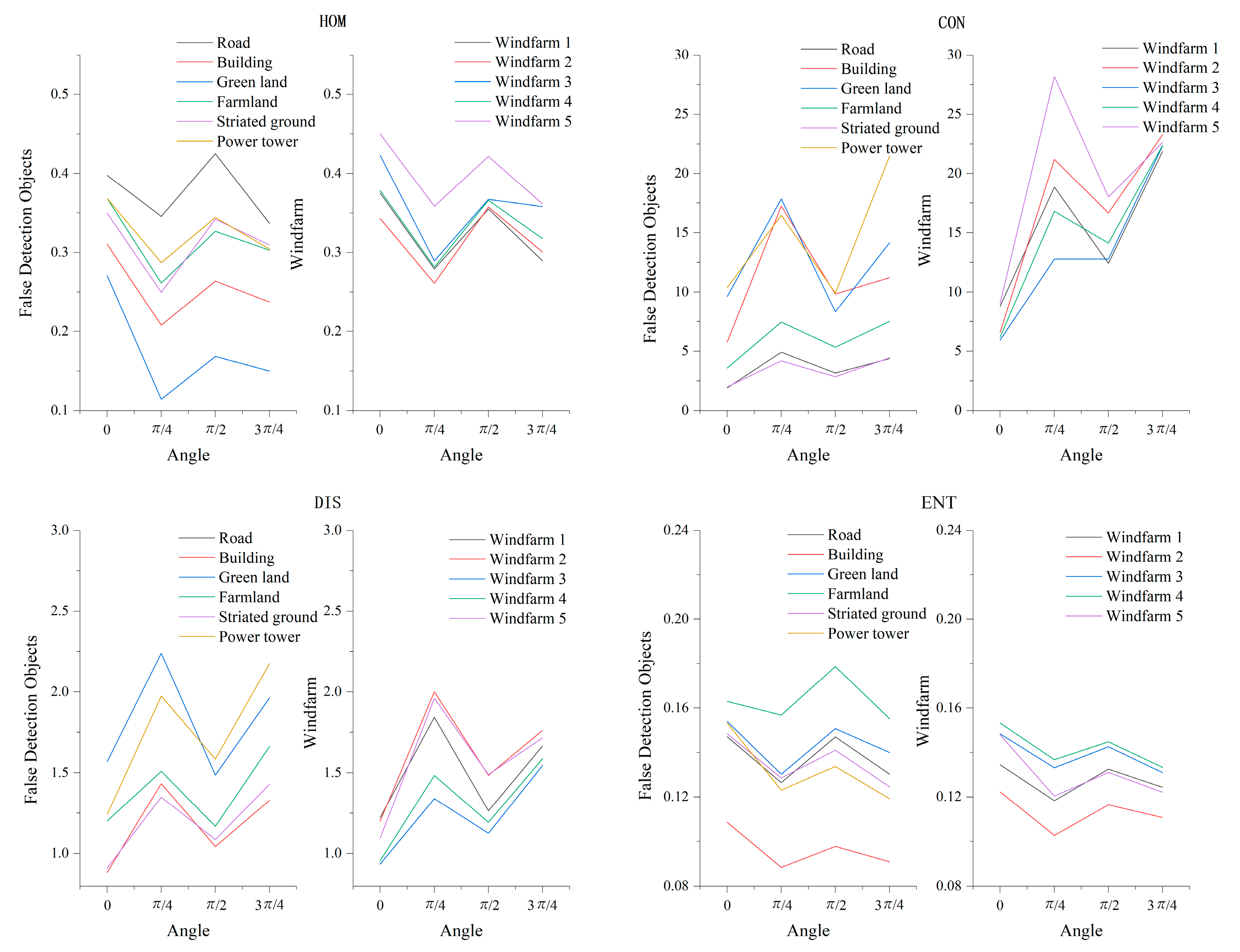
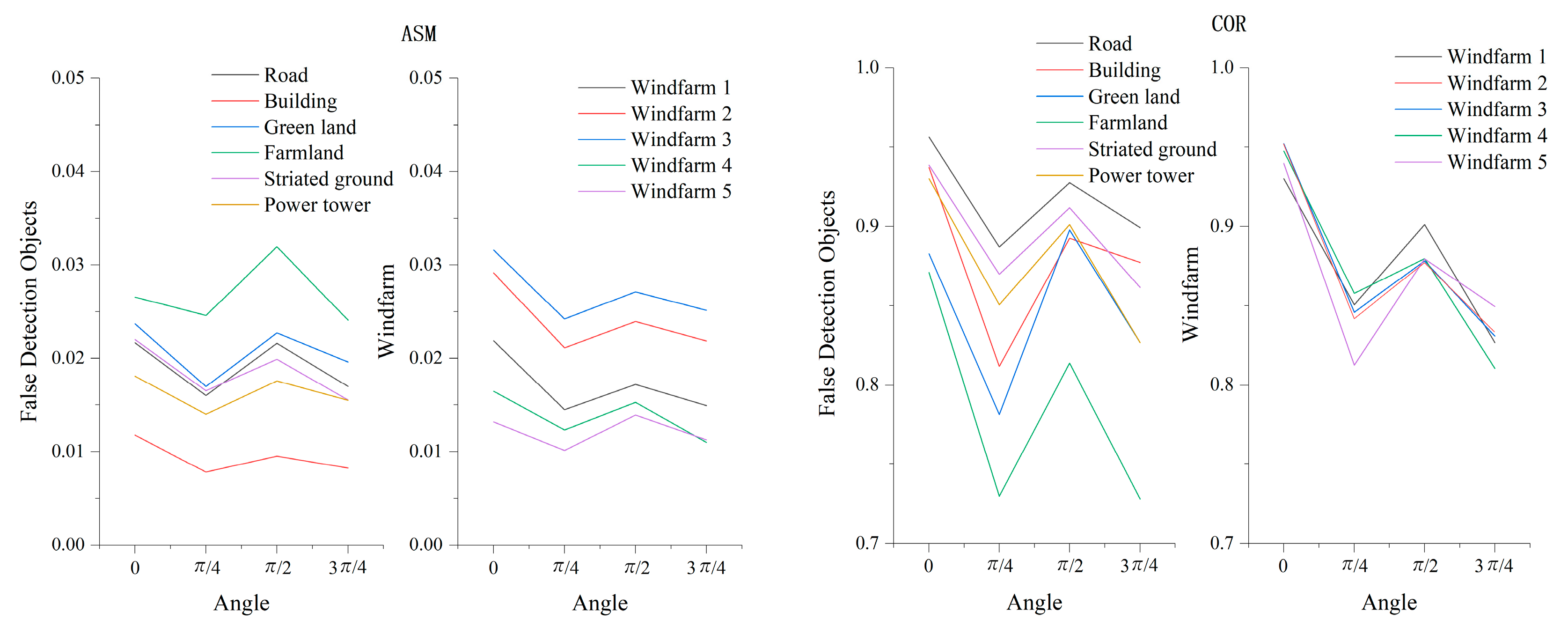
- (3)
- Image Texture Feature Selection
- (4)
- Dynamic Threshold Re-identification Method with Expert Knowledge
3.3. Evaluation Indexes for TDI
4. Results
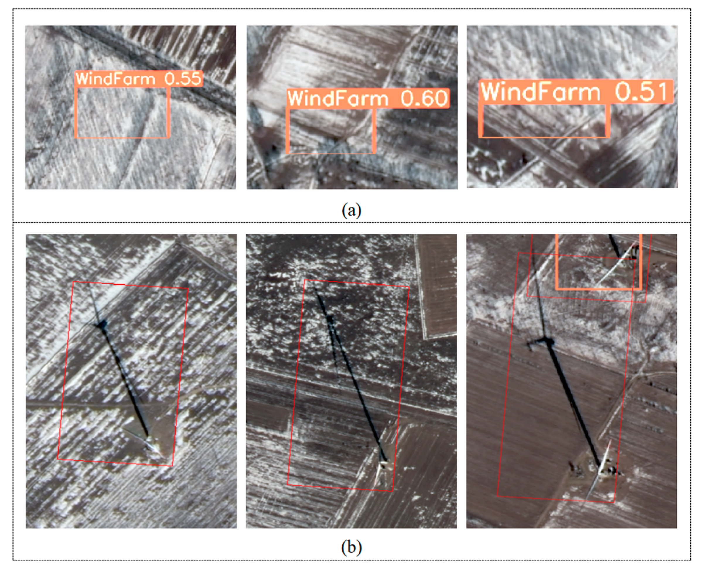
4.1. YOLOv5
4.2. YOLOv5_AC
4.3. YOLOv5_AC_CBAM
4.4. YOLOv5_AC_CBAM_Exp
5. Discussion
5.1. Effect Analysis of Quantitative Data Processing
5.2. The Overall Effectiveness of Using QRS Information
5.3. Comparison and Analysis of Different Methods
6. Conclusions
Author Contributions
Funding
Data Availability Statement
Acknowledgments
Conflicts of Interest
References
- Liu, C.; Chen, Y.; Chen, F.; Zhu, P.; Chen, L. Sliding window change point detection based dynamic network model inference framework for airport ground service process. Knowl.-Based Syst. 2022, 238, 107701. [Google Scholar] [CrossRef]
- Chen, X.; Jiang, W.; Qi, H.; Liu, M.; Ma, H.; Yu, P.L.; Wen, Y.; Han, Z.; Zhang, S.; Cao, G. Adaptive meta-knowledge transfer network for few-shot object detection in very high resolution remote sensing images. J. Appl. Earth Obs. Geoinf. 2024, 127, 103675. [Google Scholar] [CrossRef]
- Li, G.; Bai, Z.; Liu, Z.; Zhang, X.; Ling, H. Salient Object Detection in Optical Remote Sensing Images Driven by Transformer. IEEE Trans. Image Process. 2023, 32, 5257–5269. [Google Scholar] [CrossRef] [PubMed]
- Vu, B.N.; Bi, J.; Wang, W.; Huff, A.; Kondragunta, S.; Liu, Y. Application of geostationary satellite and high-resolution meteorology data in estimating hourly PM2.5 levels during the Camp Fire episode in California. Remote Sens. Environ. 2022, 271, 112890. [Google Scholar] [CrossRef] [PubMed]
- Yurtseven, H.; Yener, H. Using of high-resolution satellite images in object-based image analysis. Eurasian J. For. Sci. 2019, 7, 187–204. [Google Scholar] [CrossRef]
- Başeski, E. Heliport Detection Using Artificial Neural Networks. Photogramm. Eng. Remote Sens. 2020, 86, 541–546. [Google Scholar] [CrossRef]
- Raghavi, K. Novel Method for Detection of Ship Docked in Harbor in High Resolution Remote Sensing Image. Indones. J. Electr. Eng. Comput. Sci. 2018, 9, 12–14. [Google Scholar] [CrossRef]
- Liu, Q.; Xiang, X.; Wang, Y.; Luo, Z.; Fang, F. Aircraft detection in remote sensing image based on corner clustering and deep learning. Eng. Appl. Artif. Intell. 2020, 87, 103333. [Google Scholar] [CrossRef]
- Li, B.; Xie, X.; Wei, X.; Tang, W. Ship detection and classification from optical remote sensing images: A survey. Chin. J. Aeronaut. 2020, 34, 145–163. [Google Scholar] [CrossRef]
- Wu, W. Quantized Gromov-Hausdorff distance. J. Funct. Anal. 2006, 238, 58–98. [Google Scholar] [CrossRef]
- Harel, J.; Koch, C.; Perona, P. Graph-based visual saliency. In Proceedings of the Neural Information Processing Systems (NIPS), Vancouver, BC, Canada, 4 December 2006. [Google Scholar]
- Zhang, R.; Xu, L.; Yu, Z.; Shi, Y.; Mu, C.; Xu, M. Deep-IRTarget: An Automatic Target Detector in Infrared Imagery Using Dual-Domain Feature Extraction and Allocation. IEEE Trans. Multimedia. 2022, 24, 1735–1749. [Google Scholar] [CrossRef]
- Wu, Q.; Li, Y.; Huang, W.; Chen, Q.; Wu, Y. C3TB-YOLOv5: Integrated YOLOv5 with transformer for object detection in high-resolution remote sensing images. Int. J. Remote Sens. 2024, 45, 2622–2650. [Google Scholar] [CrossRef]
- Sun, X.; Wang, P.; Lu, W.; Zhu, Z.; Lu, X.; He, Q.; Li, J.; Rong, X.; Yang, Z.; Chang, H.; et al. RingMo: A Remote Sensing Foundation Model with Masked Image Modeling. IEEE Trans. Geosci. Remote Sens. 2022, 61, 99. [Google Scholar] [CrossRef]
- Cao, Z.; Jiang, L.; Yue, P.; Gong, J.; Hu, X.; Liu, S.; Tan, H.; Liu, C.; Shangguan, B.; Yu, D. A large scale training sample database system for intelligent interpretation of remote sensing imagery. Geo-Spat. Inf. Sci. 2023, 27, 1489–1508. [Google Scholar] [CrossRef]
- Li, K.; Wan, G.; Cheng, G.; Meng, L.; Han, J. Object detection in optical remote sensing images: A survey and a new benchmark. ISPRS J. Photogramm. Remote Sens. 2020, 159, 296–307. [Google Scholar] [CrossRef]
- Zhang, R.; Liu, G.; Zhang, Q.; Lu, X.; Dian, R.; Yang, Y.; Xu, L. Detail-Aware Network for Infrared Image Enhancement. IEEE Trans. Geosci. Remote Sens. 2025, 63, 50003. [Google Scholar] [CrossRef]
- Lou, P.; Fu, B.; Lin, X.; Tang, T.; Bi, L. Quantitative Remote Sensing Analysis of Thermal Environment Changes in the Main Urban Area of Guilin Based on Gee. Int. Arch. Photogramm. Remote Sens. Spat. Inf. Sci. 2020, 42, 881–888. [Google Scholar] [CrossRef]
- Khaleal, F.M.; El-Bialy, M.Z.; Saleh, G.M.; Lasheen ES, R.; Kamar, M.S.; Omar, M.M.; Abdelaal, A. Assessing environmental and radiological impacts and lithological mapping of beryl-bearing rocks in Egypt using high-resolution sentinel-2 remote sensing images. Sci. Rep. 2023, 13, 11497. [Google Scholar] [CrossRef]
- Zhang, R.; Tan, J.; Cao, Z.; Xu, L.; Liu, Y.; Si, L.; Sun, F. Part-Aware Correlation Networks for Few-Shot Learning. IEEE Trans. Multimedia. 2024, 26, 9527–9538. [Google Scholar] [CrossRef]
- Chen, J.; Yue, A.; Wang, C.; Huang, Q.; Chen, J.; Meng, Y.; He, D. Wind turbine extraction from high spatial resolution remote sensing images based on saliency detection. J. Appl. Remote Sens. 2018, 12, 016041. [Google Scholar] [CrossRef]
- Bian, L.; Li, B.; Wang, J.; Gao, Z. Multi-branch stacking remote sensing image target detection based on YOLOv5. Egypt. J. Remote Sens. 2023, 26, 999–1008. [Google Scholar] [CrossRef]
- Jha, S.S.; Kumar, M.; Nidamanuri, R.R. Multi-platform optical remote sensing dataset for target detection. Data Brief. 2020, 33, 106362. [Google Scholar] [CrossRef] [PubMed]
- Chen, H.; Zhang, L.; Ma, J.; Zhang, J. Target Heat-map Network: An End-to-end Deep Network for Target Detection in Remote Sensing Images. Neurocomputing 2018, 331, 375–387. [Google Scholar] [CrossRef]
- Yu, X.; Hoff, L.E.; Reed, I.S.; Chen, A.M.; Stotts, L.B. Automatic target detection and recognition in multiband imagery: A unified ML detection and estimation approach. IEEE T. Image Process. 1997, 6, 143–156. [Google Scholar] [CrossRef]
- Xie, W.; Zhang, J.; Lei, J.; Li, Y.; Jia, X. Self-spectral learning with GAN based spectral-spatial target detection for hyperspectral image. Neural Netw. 2021, 142, 375–387. [Google Scholar] [CrossRef]
- Hang, R.; Liu, Q.; Hong, D.; Ghamisi, P. Cascaded recurrent neural networks for hyperspectral image classification. IEEE Trans. Geosci. Remote Sens. 2019, 57, 5384–5394. [Google Scholar] [CrossRef]
- Zhang, L.; Huang, X.; Huang, B.; Li, P. A pixel shape index coupled with spectral information for classification of high spatial resolution remotely sensed imagery. IEEE Trans. Geosci. Remote Sens. 2006, 44, 2950–2961. [Google Scholar] [CrossRef]
- Barbato, M.P.; Piccoli, F.; Napoletano, P. Ticino: A multi-modal remote sensing dataset for semantic segmentation. Exp. Sys. Appl. 2024, 249, 123600. [Google Scholar] [CrossRef]
- Hong, D.; Zhang, B.; Li, X.; Li, Y.; Li, C.; Yao, J.; Yokoya, N.; Li, H.; Ghamisi, P.; Jia, X.; et al. SpectralGPT: Spectral Remote Sensing Foundation Model. IEEE Trans. Pattern Anal. Mach. Intell. 2024, 46, 5227–5244. [Google Scholar] [CrossRef] [PubMed]
- Yang, H.; Wang, Z.; Cao, J.; Wu, Q.; Zhang, B. Estimating soil salinity using Gaofen-2 imagery: A novel application of combined spectral and textural features. Environ. Res. 2022, 217, 114870. [Google Scholar] [CrossRef] [PubMed]
- Ren, B.; Ma, S.; Hou, B.; Hong, D.; Chanussot, J.; Wang, J.; Jiao, L. A dual-stream high resolution network: Deep fusion of GF-2 and GF-3 data for land cover classification. Int. J. Appl. Earth Obs. Geoinf. 2022, 112, 102896. [Google Scholar] [CrossRef]
- Li, Y.; Wang, C.; Wright, A.; Liu, H.; Zhang, H.; Zong, Y. Combination of GF-2 high spatial resolution imagery and land surface factors for predicting soil salinity of muddy coasts. Catena 2021, 202, 105304. [Google Scholar] [CrossRef]
- Liu, C.C.; Chen, P.L. Automatic extraction of ground control regions and orthorectification of remote sensing imagery. Opt. Express. 2009, 17, 7970–7984. [Google Scholar] [CrossRef]
- Liu, S.; Zhang, Y.; Zhao, L.; Chen, X.; Zhou, R.; Zheng, F.; Li, Z.; Li, J.; Yang, H.; Li, H.; et al. QUantitative and Automatic Atmospheric Correction (QUAAC): Application and Validation. Sensors 2022, 22, 3280. [Google Scholar] [CrossRef]
- Liu, G.; Wang, Y.; Guo, L.; Ma, C. Research on fusion of GF-6 imagery and quality evaluation. E3S Web Conf. 2020, 165, 03016. [Google Scholar] [CrossRef]
- Zi, N.; Li, X.M.; Gade, M.; Fu, H.; Min, S. Ocean eddy detection based on YOLO deep learning algorithm by synthetic aperture radar data. Remote Sens. Environ. 2024, 307, 114139. [Google Scholar] [CrossRef]
- Zhang, Y.; Ye, M.; Zhu, G.; Liu, Y.; Guo, P.; Yan, J. FFCA-YOLO for Small Object Detection in Remote Sensing Images. IEEE Trans. Geosci. Remote Sens. 2024, 62, 1–15. [Google Scholar] [CrossRef]
- Zhang, W.; Liu, Z.; Zhou, S.; Qi, W.; Wu, X.; Zhang, T.; Han, L. LS-YOLO: A Novel Model for Detecting Multi-Scale Landslides with Remote Sensing Images. IEEE J. Sel. Top. Appl. Earth Observ. Remote Sens. 2024, 17, 4952–4965. [Google Scholar] [CrossRef]
- Yu, L.; Qian, M.; Chen, Q.; Sun, F.; Pan, J. An improved YOLOv5 model: Application to mixed impurities detection for walnut kernels. Foods 2023, 12, 624. [Google Scholar] [CrossRef]
- Yin, M.; Chen, Z.; Zhang, C. A CNN-Transformer Network Combining CBAM for Change Detection in High-Resolution Remote Sensing Images. Remote Sens. 2023, 15, 2406. [Google Scholar] [CrossRef]
- Guo, Y.; Aggrey, S.E.; Yang, X.; Oladeinde, A.; Qiao, Y.; Chai, L. Detecting broiler chickens on litter floor with the YOLOv5-CBAM deep learning model. Artif. Intell. Agric. 2023, 9, 36–45. [Google Scholar] [CrossRef]
- Woo, S.; Park, J.; Lee, J.Y.; Kweon, I.S. Cbam: Convolutional block attention module. In Proceedings of the European Conference on Computer Vision (ECCV), Munich, Germany, 8 September 2018. [Google Scholar]
- Haralick, R.M.; Shanmugam, K.; Dinstein, I.H. Textural features for image classification. IEEE Trans. Syst. Man. Cybern. 1973, 6, 610–621. [Google Scholar] [CrossRef]
- Hu, J.; Wei, Y.; Chen, W.; Zhi, X.; Zhang, W. CM-YOLO: Typical Object Detection Method in Remote Sensing Cloud and Mist Scene Images. Remote Sens. 2025, 17, 125. [Google Scholar] [CrossRef]
- Wu, Z.; Wu, D.; Li, N.; Chen, W.; Yuan, J.; Yu, X.; Guo, Y. CBGS-YOLO: A Lightweight Network for Detecting Small Targets in Remote Sensing Images Based on a Double Attention Mechanism. Remote Sens. 2025, 17, 109. [Google Scholar] [CrossRef]
- Zhou, H.; Wu, S.; Xu, Z.; Sun, H. Automatic detection of standing dead trees based on improved YOLOv7 from airborne remote sensing imagery. Front. Plant Sci. 2024, 15, 1278161. [Google Scholar] [CrossRef]
- Hui, Y.; Wang, J.; Li, B. DSAA-YOLO: UAV remote sensing small target recognition algorithm for YOLOV7 based on dense residual super-resolution and anchor frame adaptive regression strategy. J. King Saud. Univ. Comput. Inf. Sci. 2024, 36, 101863. [Google Scholar] [CrossRef]
- Ma, D.; Liu, B.; Huang, Q.; Zhang, Q. MwdpNet: Towards improving the recognition accuracy of tiny targets in high-resolution remote sensing image. Sci. Rep. 2023, 13, 13890. [Google Scholar] [CrossRef]
- Lin, S. Automatic recognition and detection of building targets in urban remote sensing images using an improved regional convolutional neural network algorithm. Cogn. Comput. Syst. 2023, 5, 132–137. [Google Scholar] [CrossRef]
- Sun, X.; Wang, P.; Yan, Z.; Xu, F.; Wang, R.; Diao, W.; Chen, J.; Li, J.; Feng, Y.; Xu, T.; et al. FAIR1M: A benchmark dataset for fine-grained object recognition in high-resolution remote sensing imagery. ISPRS J. Photogramm. Remote Sens. 2022, 184, 116–130. [Google Scholar] [CrossRef]


| Payload | Band Number | Spectral Band | Spatial Resolution |
|---|---|---|---|
| Multispectral and Panchromatic Cameras | 1 | 0.45 µm–0.90 µm | 1 m |
| 2 | 0.45 µm–0.52 µm | 4 m | |
| 3 | 0.52 µm–0.59 µm | ||
| 4 | 0.63 µm–0.69 µm | ||
| 5 | 0.77 µm–0.89 µm |
| Confidence Threshold | (%) |
|---|---|
| 0.75 | 95.7 |
| 0.80 | 100 |
| 0.85 | 100 |
| 0.90 | 100 |
| Model | Whether to Perform Quantitative AC | ||||
|---|---|---|---|---|---|
| YOLOv5 | No | 0.944 | 0.925 | 0.938 | 0.735 |
| YOLOv5_AC | Yes | 0.957 | 0.946 | 0.953 | 0.744 |
| Model | Total Number of True Targets | (%) | (%) | (%) | |||
|---|---|---|---|---|---|---|---|
| YOLOv5 | 1912 | 1875 | 158 | 37 | 90.5 | 7.8 | 2.0 |
| YOLOv5_AC | 1912 | 1897 | 133 | 15 | 92.7 | 6.6 | 0.78 |
| YOLOv5_AC_CBAM | 1912 | 1898 | 124 | 14 | 93.2 | 6.1 | 0.73 |
| YOLOv5_AC_CBAM_Exp | 1912 | 1891 | 30 | 21 | 97.4 | 1.6 | 1.1 |
| Model | ||||
|---|---|---|---|---|
| FasterRCNN | 0.934 | 0.943 | 0.937 | 0.675 |
| YOLOv7 | 0.935 | 0.944 | 0.938 | 0.670 |
| YOLOv5_AC | 0.957 | 0.946 | 0.953 | 0.744 |
| YOLOv5_AC_CBAM | 0.960 | 0.949 | 0.957 | 0.746 |
| Features | Total Number of Real Targets | (%) | (%) | (%) | |||
|---|---|---|---|---|---|---|---|
| No | 1912 | 1898 | 124 | 14 | 93.2 | 6.1 | 0.7 |
| Fa | 1912 | 1891 | 49 | 21 | 96.4 | 2.5 | 1.1 |
| Fb | 1912 | 1896 | 93 | 16 | 94.6 | 4.7 | 0.8 |
| Fc | 1912 | 1897 | 72 | 15 | 95.6 | 3.7 | 0.8 |
| Fa + Fb | 1912 | 1891 | 35 | 21 | 97.1 | 1.8 | 1.1 |
| Fa + Fc | 1912 | 1891 | 37 | 21 | 97.0 | 1.9 | 1.1 |
| Fb + Fc | 1912 | 1894 | 59 | 18 | 96.1 | 3.0 | 0.9 |
| Fa + Fb + Fc | 1912 | 1891 | 30 | 21 | 97.4 | 1.6 | 1.1 |
Disclaimer/Publisher’s Note: The statements, opinions and data contained in all publications are solely those of the individual author(s) and contributor(s) and not of MDPI and/or the editor(s). MDPI and/or the editor(s) disclaim responsibility for any injury to people or property resulting from any ideas, methods, instructions or products referred to in the content. |
© 2025 by the authors. Licensee MDPI, Basel, Switzerland. This article is an open access article distributed under the terms and conditions of the Creative Commons Attribution (CC BY) license (https://creativecommons.org/licenses/by/4.0/).
Share and Cite
Chen, X.; Zhang, Y.; Xue, W.; Liu, S.; Li, J.; Meng, L.; Yang, J.; Mi, X.; Wan, W.; Meng, Q. Quantitative Remote Sensing Supporting Deep Learning Target Identification: A Case Study of Wind Turbines. Remote Sens. 2025, 17, 733. https://doi.org/10.3390/rs17050733
Chen X, Zhang Y, Xue W, Liu S, Li J, Meng L, Yang J, Mi X, Wan W, Meng Q. Quantitative Remote Sensing Supporting Deep Learning Target Identification: A Case Study of Wind Turbines. Remote Sensing. 2025; 17(5):733. https://doi.org/10.3390/rs17050733
Chicago/Turabian StyleChen, Xingfeng, Yunli Zhang, Wu Xue, Shumin Liu, Jiaguo Li, Lei Meng, Jian Yang, Xiaofei Mi, Wei Wan, and Qingyan Meng. 2025. "Quantitative Remote Sensing Supporting Deep Learning Target Identification: A Case Study of Wind Turbines" Remote Sensing 17, no. 5: 733. https://doi.org/10.3390/rs17050733
APA StyleChen, X., Zhang, Y., Xue, W., Liu, S., Li, J., Meng, L., Yang, J., Mi, X., Wan, W., & Meng, Q. (2025). Quantitative Remote Sensing Supporting Deep Learning Target Identification: A Case Study of Wind Turbines. Remote Sensing, 17(5), 733. https://doi.org/10.3390/rs17050733