A Fast Algorithm for Matching AIS Trajectories with Radar Point Data in Complex Environments

Abstract

In high-traffic port areas, vessel traffic-management systems (VTMS) are essential for managing ship movements and preventing collisions. However, inaccuracies and omissions in the Automatic Identification System (AIS), along with frequent false tracks generated by radar false alarms in complex environments, can compromise VTMS stability. To address the challenges of establishing consistent navigation and improving trajectory quality, this study introduces a novel method to directly identify AIS-matched trajectories from radar plots. This approach treats radar points as probability clouds, generating a multi-dimensional information layer by stacking these clouds after differential transformations based on AIS data. The resulting layer undergoes filtering and clustering to extract point sets that align with AIS data, effectively isolating matching trajectories. The algorithm, validated with simulated data, rapidly identifies target trajectories amid extensive interference without requiring strict parameter adjustments. In measured data, the algorithm rapidly provides matching trajectories, although further human judgment is still required due to the potential absence of true values in measured data.

1. Introduction

Currently, marine transportation constitutes over 90% of the global cargo transportation volume [1], playing a pivotal role in international logistics. However, coastal, port, and inland waterway areas exhibit high vessel traffic density and complex navigational scenarios [2], posing considerable challenges to safe navigation and elevating the risk of collisions [3].

Vessel traffic-management systems primarily rely on two subsystems: AIS and radar system [4]. AIS data provide high accuracy and extensive coverage; however, AIS data arrival is unpredictable and random [5,6], especially in high-density traffic areas, where extended data gaps may occur [7]. In contrast, radar-based tracking serves as a supplementary source; however, data from radar systems, including shipborne radar, is susceptible to false alarms and missed detections. This, coupled with considerable variance in radar readings, can lead to missed and incorrect matches [8].

A common approach involves processing radar and AIS data separately within distributed systems to generate high-quality tracking information [9,10]. Subsequently, these data are matched and fused, as illustrated in Figure 1.

Traditional research in this field has relied on signal-processing and data-analysis techniques, including fuzzy decision theory [11,12], maximum likelihood estimation [13], Hough transform [14,15], and Kalman filtering [16,17], to achieve stable and precise data. However, data fusion typically occurs at a later stage, without fully leveraging the distinct characteristics of both sensor types. This approach introduces unnecessary computational load during the track-building phase, and due to the inconsistency in track quality, there may be a high incidence of missed or incorrect tracks in complex environments.

This paper presents a novel approach that enables direct matching of AIS data and radar plot data in complex situations. The specific process is illustrated in Figure 2:

In Section 2, each step of the process illustrated in Figure 2 is described in detail. Due to practical application requirements, the step of “create radar point probability clouds” has been moved up to facilitate the rapid extraction of parameters for different AIS data based on various indices. In the paper, this step is discussed in Section 2.3.

Section 2.1 presents the strategies adopted for time alignment. Depending on the time interval, two algorithms are employed: the Spherical Linear Interpolation (SLERP) algorithm [18], proposed by Ken Shoemake in 1985, and the Catmull–Rom algorithm [19], proposed by Edwin Catmull and Raphael Rom in 1974.

Section 2.2 explains how the problem of trajectory establishment is transformed into the “Smallest Color-Spanning Circle” problem through “difference transformation” and “layer stacking”. It also demonstrates that by incorporating additional parameters, the process of trajectory establishment can be included as well.

Section 2.3 describes how to construct a probability cloud map and extract the required parameters from it. In this paper, two parameters are extracted: the deviation of the trajectory from the true value and the variance of the trajectory, which correspond to the dashed parts in the flowchart.

As Section 2.4 shows, a simple nearest neighbor algorithm is employed in this paper to extract the corresponding radar trajectory based on these parameters, which are demonstrated in Section 3. Section 4 analyzes the impact of errors and hyperparameters, suggesting directions for future improvements.

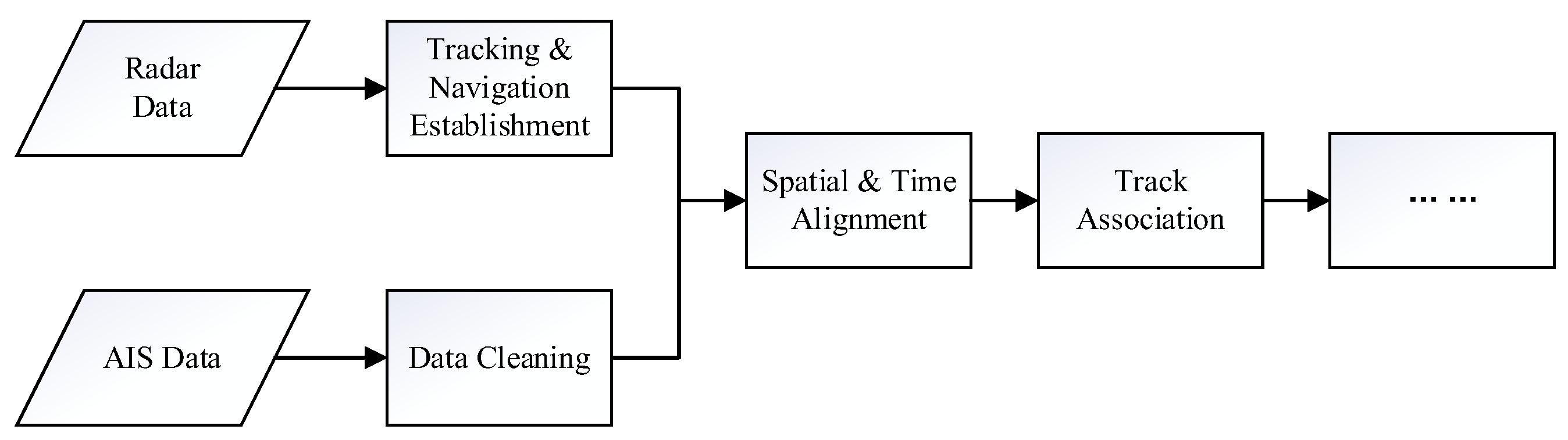
2. Materials and Methods

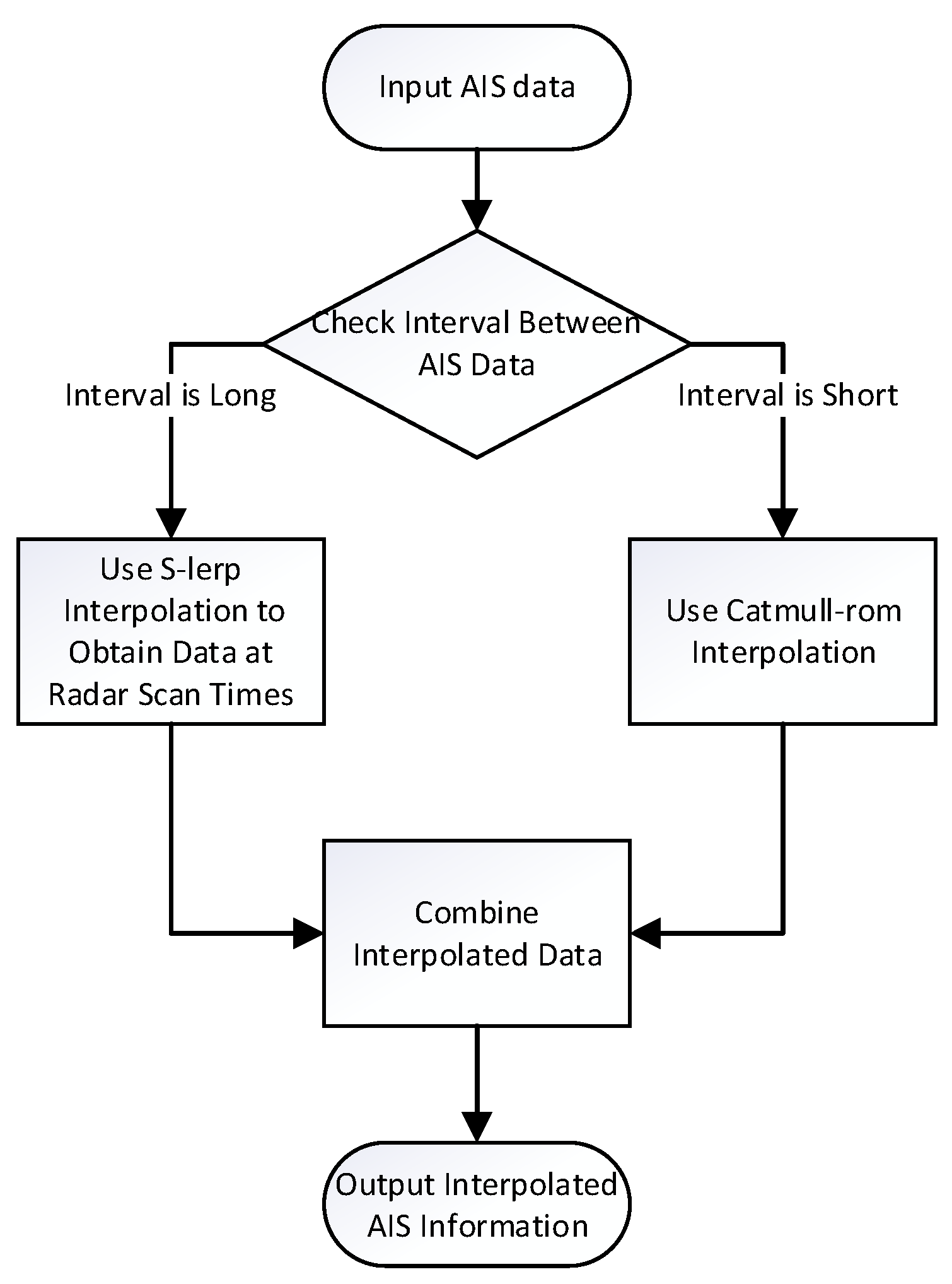
2.1. Time and Spatial Unification

Due to the differences in how AIS and radar acquire information [16], they operate in different coordinate systems, necessitating spatial unification.

AIS data include longitude and latitude, while radar data consist of distance and angle. A unified coordinate system is necessary for effective comparison.

This paper chooses latitude and longitude for alignment between the two, projecting the radar’s polar coordinates onto this coordinate system. In the subsequent steps of synchronous navigation and matching, the heading and speed coordinates need to be introduced and transformed.

Given that AIS and radar acquire information through different methods—radar through active scanning and AIS through individual ships uploading data—the acquisition intervals usually differ, making time unification necessary. Radar data are generally collected at regular intervals, which are typically longer than those for AIS data. AIS data upload times are irregular and may experience packet loss, as shown in Figure 3:

Given that AIS data-acquisition times are governed by the transmission schedules of vessels, while radar data are collected at consistent intervals, it is standard practice to interpolate AIS trajectory data to synchronize them with radar scan intervals.

Additionally, AIS employs SOTDMA (Self-Organized Time Division Multiple Access), which may lead to the loss of AIS messages under adverse weather conditions or high traffic density, as well as potential data loss due to time slot conflicts between different AIS devices [20].

Given that the accuracy of this method heavily relies on the precision of AIS data, using a single interpolation method to align all points may introduce unnecessary errors. Ling-zhi Sang et al. proposed a method of employing different interpolation functions for different segments to obtain more accurate AIS data [21]. We also adopt varying interpolation schemes based on the temporal characteristics of the AIS data.

Linear interpolation does not account for the continuity of a vessel’s speed, leading to abrupt speed changes. While spline interpolation considers speed continuity, the introduction of higher-order polynomials may result in an unrealistic trajectory when AIS data are continuously lost. The actual trajectory is influenced by various factors, such as the captain’s navigation habits and sea conditions [22].

As shown in Figure 4, with known heading and position, the influence of the heading on the trajectory fitting should diminish as the distance between points increases.

Considering this scenario, the following strategy is employed for interpolation in this paper.

When AIS data are continuous or there is minimal data loss, priority is given to maintaining the continuity of the vessel’s speed, using spline interpolation. However, when there is significant data loss, the interpolation method takes the Earth’s curvature into account, selecting the shortest path using SLERP interpolation, as shown in Figure 5.

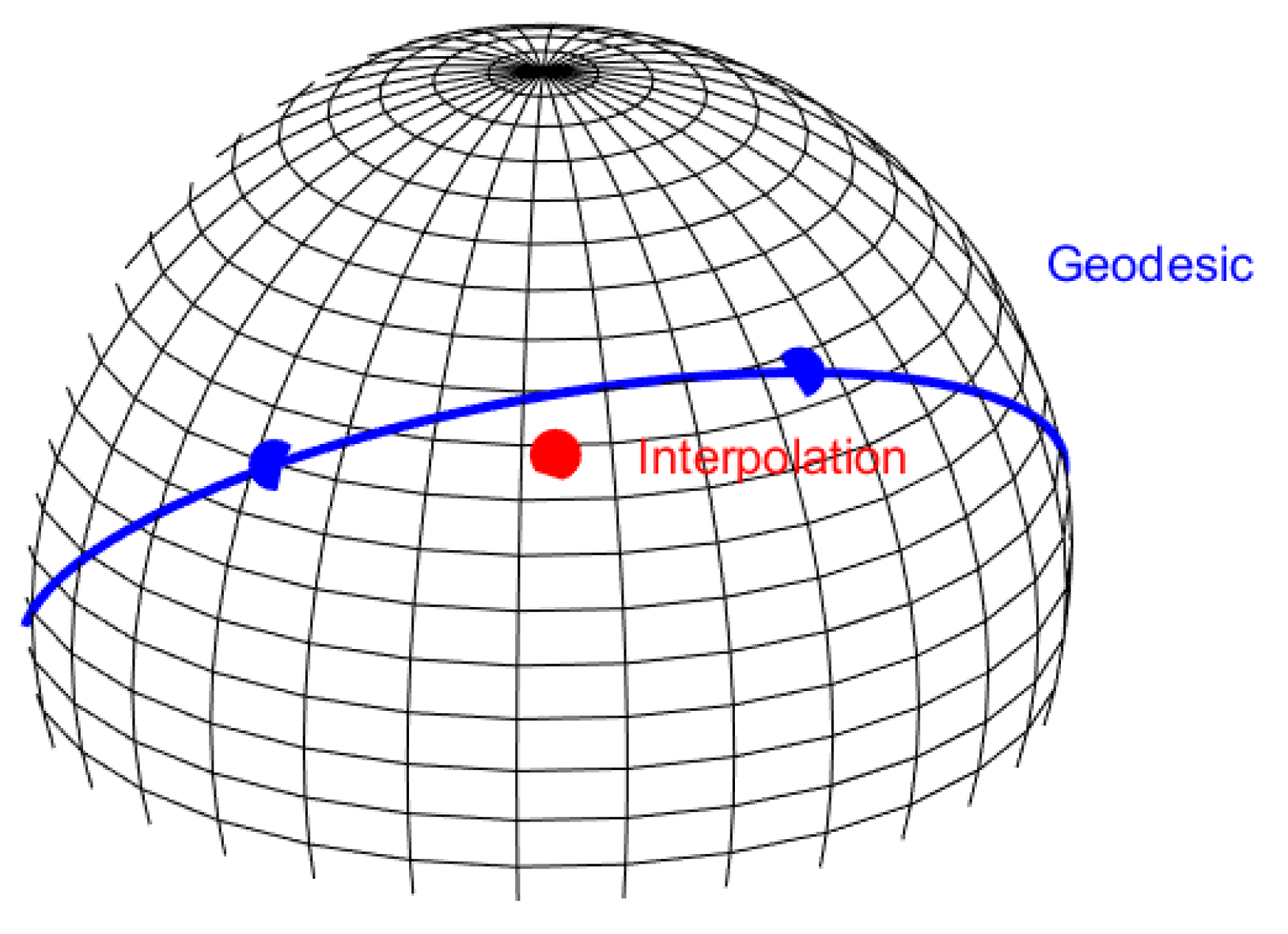
2.1.1. SLERP Interpolation

• Error Analysis of Interpolation Methods

When AIS data are continuously lost and the distance between two points is relatively large, consideration of the Earth’s curvature becomes necessary for selecting the shortest path. Most current research conducts trajectory analysis on a zero-curvature plane [23,24]. However, The shortest distance between two points on a sphere is not a straight line but a geodesic [25].

When treating the Earth as a sphere, the geodesic (the term “geodesic” was coined by Bernhard Riemann, and it refers to the shortest path between two points on a curved surface; this concept originates from differential geometry, a branch of mathematics that focuses on the study of curves and surfaces) is the intersection of the plane formed by the two points and the sphere’s center. However, directly performing linear interpolation on latitude and longitude introduces errors.

The relationship between the position of the linear interpolation point in latitude and longitude and its corresponding geodesic position is depicted in Figure 6.

Consequently, to minimize interpolation errors for the shortest path, especially when the distance between two points is significant, this paper adopts the S-lerp method [18,26]. Furthermore, it provides a straightforward proof through formulas to explain why this algorithm is suitable for latitude and longitude interpolation.

• SLERP-Based Latitude and Longitude Interpolation

SLERP interpolation utilizes quaternions. A quaternion $q=w+xi+yj+zk$ is an extension of complex numbers with the following properties:

$$\left\{\begin{array}{l}{i}^2=j^2=k^2=ijk=-1\\ ij=-ji=k\\ ji=-kj=i\\ ki=-ij=j\end{array}\right.$$

(1)

In academia, the imaginary components $i,j,k$ of the quaternion are extracted and correspond to the coordinate system $(x,y,z)$, respectively, while the scalar component is conventionally set to zero.

Let $P$ be a point in the Cartesian coordinate system, with the vector from the origin to point $P$ denoted as $\overrightarrow{O{P}_{old}}$. Suppose this vector is rotated by an angle $\theta$ around a unit vector $\overrightarrow{u}=[u_x,u_y,u_z]$ that passes through the origin. When $P$ is perpendicular to the unit vector $\overrightarrow{u}$, the results rotation can be expressed in the Cartesian coordinate system as follows:

$$\overrightarrow{O{P}_{new}}=\mathit{cos}\left(\theta \right)\cdot \overrightarrow{O{P}_{old}}+\mathit{sin}\left(\theta \right)\cdot \left(\overrightarrow{u}\times \overrightarrow{O{P}_{old}}\right)$$

(2)

Here, $\overrightarrow{O{P}_{new}}$ represents the result of rotating the vector around the axis $\overrightarrow{u}$. To transform the point in the Cartesian coordinate system into a quaternion, we have $q_P=0+P_{x}i+P_{y}j+P_{z}k$. Similarly, when $\overrightarrow{u}$ is also converted into a quaternion $q_u=0+u_{x}i+u_{y}j+u_{z}k$, it can be observed that the quaternion representation $q_v$ of the vector $\overrightarrow{V}=\overrightarrow{O{P}_{old}}\times \overrightarrow{u}$ is the product of the quaternion representation of $\overrightarrow{u}$ and $\overrightarrow{O{P}_{old}}$, as shown in Equation (3):

$$q_v=\left(0+u_{x}i+u_{y}j+u_{z}k\right)\left(0+P_{x}i+P_{y}j+P_{z}k\right)$$

(3)

At this point, the rotation can be simply represented as a left multiplication by a quaternion. Let $q_p^{\prime }$ be the quaternion representing the point $P$ after it has been rotated by an angle $\theta$ around the unit vector $\overrightarrow{u}$. this results in the following expression:

$$q_p^{\prime }=\left(\cos \theta +sin\theta \cdot u_{x}i+sin\theta \cdot u_{y}j+\sin \theta \cdot u_{z}k\right)\cdot q_p$$

(4)

Hence, considering the interpolation between two points $P_1$ and $P_2$, on a sphere, by adjusting the value of $\theta$, the rotation from $\overrightarrow{O{P}_1}$ to $\overrightarrow{O{P}_2}$ can be smoothly represented in the SLERP algorithm [26].

Let $q_t$ be the quaternion of the interpolation point, with the known adjacent points in the trajectory being $q_0$ and $q_1$. The SLERP interpolation formula is shown in Equation (5):

$$q_t={\displaystyle \frac{\mathit{sin}\left(1-t\right)\theta }{sin\theta }}{q}_0+{\displaystyle \frac{\mathit{sin}t\theta }{sin\theta }}{q}_1$$

(5)

where $t\in \left[\mathrm{0,1}\right]$ is a proportional coefficient of the interpolation point, which is obtained from Equation (6):

$$t={\displaystyle \frac{t_{radar}-t_{ais,\left(k-1\right)}}{t_{ais,k}-t_{ais,\left(k-1\right)}}}$$

(6)

where $t_{radar}\in [t_{ais,\left(k-1\right)},t_{ais,k}]$ represents the radar scan time, with $t_{ais,k},t_{ais,(k-1)}$ being the corresponding times for the $k$-th and $(k-1)$-th points in the AIS sequence.

With the introduction of SLERP, the overall processing workflow can be summarized as follows:

• Convert latitude and longitude to a quaternion-based Cartesian system.
• Apply SLERP interpolation.
• Reconvert the results to latitude and longitude.

The Earth is considered a sphere with its center $O$ located at the origin of a Cartesian coordinate system. For the two known points at times $t_{ais,(k-1)}$ and $t_{ais,\left(k\right)}$, the corresponding quaternions $q_0$ and $q_1$ can be obtained by Equation (7):

$$\left\{\begin{array}{l}w=0\\ \begin{array}{l}x=r\cdot \mathit{cos}\left(la{t}_{rad}\right)\cdot \mathit{cos}\left(lo{n}_{rad}\right)\\ y=r\cdot \mathit{cos}\left(la{t}_{rad}\right)\cdot \mathit{sin}\left(lo{n}_{rad}\right)\\ z=r\cdot \mathit{sin}\left(la{t}_{rad}\right)\end{array}\end{array}\right.$$

(7)

Here, $la{t}_{rad},lo{n}_{rad}$ are the latitude and longitude converted to radians, while $w,x,y,z$ are the components of the quaternion $q=w+xi+yj+zk$. $r$ represents the radius of the Earth. With this, SLERP interpolation can be accomplished.

Let the quaternions for the two known points be defined as $q_0={r\cdot x}_{0}i+r\cdot y_{0}j+r\cdot z_{0}k$ and $q_1=r\cdot x_{1}i+r\cdot y_{1}j+r\cdot z_{1}k$. The interpolated quaternion $q_t$ at time $t_{radar}$ can be expressed using Equation (5), where $\theta$ is calculated from Equation (8):

$$\theta =\mathit{acos}\left(x_0{x}_1+y_0{y}_1+z_0{z}_1\right)$$

(8)

Finally, the latitude and longitude at time $t_{radar}$ can be calculated using Equation (9):

$$\left\{\begin{array}{l}\begin{array}{c}la{t}_t={\displaystyle \frac{180}{\pi }}\mathit{asin}{\displaystyle \frac{z}{r}}\\ lo{n}_t={\displaystyle \frac{180}{\pi }}\mathit{atan}{\displaystyle \frac{y}{x}}\end{array}\\ s.t.{lat}_t\in \left[-\mathrm{180,180}\right],{lon}_t\in \left[\mathrm{0,360}\right]\end{array}\right.$$

(9)

2.1.2. Catmull–Rom

The Catmull–Rom curve is a type of spline that provides smooth interpolation through a set of control points [19]. The Catmull–Rom curve is specifically designed to pass exactly through each of the given control points, while also offering the advantages of simple computation and not requiring the calculation of derivatives.

The curve is defined by a set of points and uses a parameter to determine the curve’s position between these points. The Catmull–Rom spline ensures continuity and smooth transitions between segments, making it a popular choice for creating smooth, flowing paths. And the formula is that:

$$\overrightarrow{C\left(t\right)}={\displaystyle \frac{1}{2}}[\left(2\overrightarrow{P_1}\right)-\left(\overrightarrow{P_0}-\overrightarrow{P_2}\right)t+\left(2\overrightarrow{P_0}-5\overrightarrow{P_1}+4\overrightarrow{P_2}-\overrightarrow{P_3}\right)t^2-\left(\overrightarrow{P_0}-3\overrightarrow{P_1}+3\overrightarrow{P_2}-\overrightarrow{P_3}\right)t^3]$$

(10)

where $\overrightarrow{P_0},\overrightarrow{P_1},\overrightarrow{P_2},\overrightarrow{P_3},$ are the control points, $\overrightarrow{C\left(t\right)}$ is the interpolation point. $t\in \left[\mathrm{0,1}\right]$ is a proportional coefficient of the interpolation point, which is obtained from Equation (6):

Since the Catmull–Rom method requires four control points for interpolation, if fewer than four points are available, additional points are estimated based on the direction of travel to reach the required number of points.

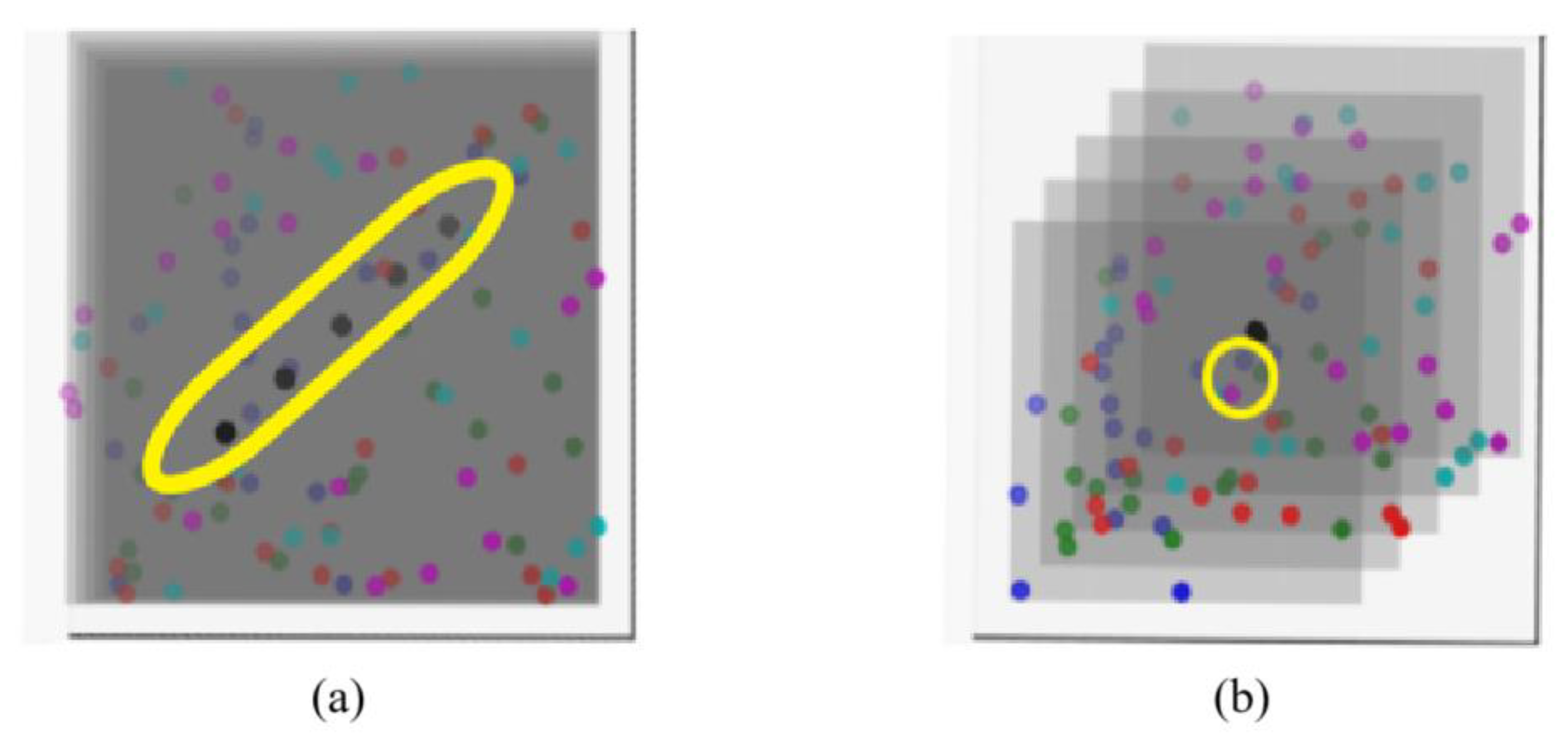
2.2. Stacking & Diffusion Transformation

When establishing radar tracks in complex environments, due to the large amount of data, traditional parallel processing approaches include clustering division and spatial division [27].

“Spatial division” adopts the idea of multi-node regional processing, dividing the processing airspace equally according to the number of processing nodes obtained. Each block is associated separately, and the main node manages the track batch numbers. This method is obviously not suitable for track establishment in complex environments, as there is a possibility of missed or incorrect divisions.

“Clustering division” adopts the idea of dynamic irregular data division. Starting from the first batch of points, it associates the next batch of points according to a threshold range, then updates the positions, and repeats this process until the association is complete. This divides the space into multiple independent autocorrelated data areas, eliminating data coupling. When the point distribution is sparse, clustering division has the advantage of eliminating errors. The general formula for clustering division can be expressed as Equation (11):

$$\overrightarrow{P_{k+1,c}}=f_k\left(\overrightarrow{P_{k,c}},co{g}_{k,set},v_{k,set}\right)$$

(11)

where $\overrightarrow{P_{k,c}}$ is the estimated value of the k-th point in the radar track, and $co{g}_{k,set}$ and $v_{k,set}$ represent the course over ground (COG) and the velocity in the COG direction of the point trace $\overrightarrow{P_{k,set}}$hat is associated with the track in the $k$-th batch of point traces. The associated point $\overrightarrow{P_{k,set}}$ can be obtained from Equation (12):

$$\overrightarrow{P_{k,set}}=\underset{P_k\in D}{\mathit{argmin}}\left(|\overrightarrow{P_k}-\overrightarrow{P_{k,c}}|\right)$$

(12)

where D is the set of all radar point traces in the $(k+1)$-th batch. In some cases, $\overrightarrow{P_{k,set}}$ may not a single point. To avoid deviations in the search, we may opt for the nearest set of the first n tracks.

When using $\overrightarrow{P_{k+1,c}}$ to associate points in the $(k+2)$-th batch of radar data to this track, if there is an error ${\delta }_k$ in the track point of the center point $\overrightarrow{P_{k,c}}$, it may lead to wrong association of points, which can further result in a series of error. This issue is particularly evident during the initial stage of track establishment [28].

The Hough Transform addresses the problem of quickly and accurately establishing target tracks in a strong clutter environment during the initial phase of track formation. It employs methods of parameter space transformation and vote accumulation. Since Smith et al. first introduced the Hough Transform to track formation [29], numerous variants have emerged, transforming the track formation problem into a feature curve detection problem [30]. However, limited by the fact that the feature curves themselves are unknown, this method can easily generate false tracks in complex environments and may miss non-linear true tracks. By incorporating AIS, this paper reduces the computational overhead during the navigation initialization phase while avoiding error propagation in complex environments. Initially, the point cloud data from each radar scan are transformed and then stacked. Subsequently, associations are made across all time-series scan points, which prevents the possibility of data drift starting from a wrong point and also reduces time complexity.

When incorporating trajectory and heading information from AIS, it becomes possible to bypass the radar initialization process and complete the initialization directly during the matching phase, thus avoiding information reuse.

2.2.1. Processing of Location Information

To uniformly represent the information from all batches, the radar scan points are stacked in the form of layers, as shown in Figure 7a. Each layer represents the result of a single radar scan, and the red dots indicate the positions of the AIS data after interpolation at the corresponding radar scan time points.

After layer stacking, all radar data and AIS data appear in the same layer. A straightforward idea is as follows: Is it possible to find a group of points resembling the red dots from the point cloud directly?

To achieve this functionality, this paper applies the transformation shown in Equation (13) to the stacked AIS data, and the result is displayed in Figure 7b.

$$\overrightarrow{P_{new,i}}=\overrightarrow{P_{old,i}}-\overrightarrow{A_i}$$

(13)

Here, $\overrightarrow{p_{old,i}}$ represents the set of all radar points scanned during the $i$-th scan, $\overrightarrow{A_i}$ represents the AIS data value at the time of the $i$-th radar scan, which is obtained through the interpolation method mentioned previously, and $\overrightarrow{P_{new,i}}$ represents the transformed radar points scanned during the $i$-th scan. For each scan, every layer undergoes a difference transformation.

Assign different colors to radar points from different batches, as shown in Figure 8a. The problem of ship track establishment is then transformed into the problem of “drawing a circle that encompasses one point of each color”, as illustrated in Figure 8b.

Here, due to our transformation, the AIS data are now located at the origin $\left(\mathrm{0,0}\right)$. We assume that the yellow circle in Figure 8b can be represented by Equation (14):

$${\left(x-x_t\right)}^2+{\left(y-y_t\right)}^2=r_t^2$$

(14)

At this point, $\sqrt{(x_t^2+y_t^2)}$ can represent the average deviation of this set of points relative to the AIS data, while $r_t^2$ can be interpreted as the shape similarity of this set of points compared to the AIS track.

If we desire the shape of the radar points to be as similar as possible to AIS points, the problem further transforms into the “Smallest Color-Spanning Circle (Smallest Color-Spanning Objects)” [31] problem. Alternatively, we can also construct a function that incorporates the average deviation to calculate a score.

In this method, it is noteworthy that since the stacked points do not involve temporal order information, the radar track establishment is no longer influenced by the sequence order, exhibiting good robustness in complex environments. The process of drawing the circle in this method involves significant computational effort. To address this issue, this paper adopts a combination of probability clouds and clustering methods. For details, please refer to Section 2.3.

2.2.2. Transformation Based on Kinematics

Furthermore, if we introduce the track and heading information from AIS data into the aforementioned method, we can actually encompass both track establishment and matching within it.

In traditional track establishment methods, radar plots are used to establish tracks, which are then matched with time-aligned AIS data, as shown in Equation (15):

$$\underset{i}{\mathit{argmin}}{‖\left[\begin{array}{c}\mathit{sin}\left({cog}_{n-1,set}\right)\\ \mathit{cos}\left({cog}_{n-1,set}\right)\end{array}\right]v_{n-1,set}+\left[\begin{array}{c}lo{n}_{n-1,c}\\ la{t}_{n-1,c}\end{array}\right]-\left[\begin{array}{c}{lon}_{i,ais}\\ la{t}_{i,ais}\end{array}\right]‖}_2$$

(15)

where ${\left(lo{n}_{i,ais},la{t}_{i,ais}\right)}^t$ represents the longitude and latitude coordinates at time n after interpolating the AIS trajectory. If we assume that the errors in AIS data are sufficiently small, then the results obtained by this method are numerically equivalent to those given by Equation (16):

$$\underset{i}{\mathit{argmin}}{‖\begin{array}{c}\begin{array}{c}\mathit{sin}\left(co{g}_{n,set}\right)\cdot v_{n,set}-\mathit{sin}\left(co{g}_{n,set}\right)\cdot v_{n,set}\\ \mathit{cos}\left(co{g}_{n,set}\right)\cdot v_{n.set}-\mathit{sin}\left(co{g}_{n,set}\right)\cdot v_{n,set}\end{array}\\ \begin{array}{c}lo{n}_{n,c}-lo{n}_{i,ais}\\ la{t}_{n,c}-la{t}_{i,ais}\end{array}\end{array}‖}_2$$

(16)

Therefore, when directly matching combinations of track, heading, longitude, and latitude under Euclidean distance to find the optimal track, it essentially encompasses the functionality of traditional methods that use radar point trace associations for track establishment.

At this point, since the information in the point $\overrightarrow{P_{k,c}}$ in Equation (11) has been extended from merely including longitude and latitude to also including heading and speed, the meaning of the distance between longitude and latitude remains the same. However, heading and speed are not comparable to longitude and latitude in the same way. Therefore, simply using the “Smallest Color-Spanning Sphere” is not appropriate. Instead, we can consider introducing coefficients a and b as shown in Equation (17) or alternatively use a rectangular prism.

$${a\left(lat-{lat}_i\right)}^2+{a\left(lon-{lon}_i\right)}^2+{b\left(\mathit{cos}\left(cog\right)v-\mathit{cos}\left(co{g}_i\right)v_i\right)}^2+b{\left(\mathit{sin}\left(cog\right)v-\mathit{sin}\left({cog}_i\right)v_i\right)}^2=r^2$$

(17)

2.3. Parameter Extraction

The previous section presented a method for simultaneously constructing and matching routes using AIS data. However, to achieve matching, there must be a way to determine the “optimal circle.” Assuming the existence of an optimal solution (true value), how can we search for it?

We know that when the search tree is sufficiently large, we can inevitably find the optimal solution (true value). According to the MIN-MAX principle, it is feasible to either first search for the distribution of all points that can be enclosed by a circle with radius r and then search for the circle closest to the center among these circles, or to first search for the top k circles closest to the center and then search for the circle with the smallest radius among these circles—as long as the search tree is sufficiently large. However, we don’t always have a sufficiently large search tree, and the optimal solution of the scoring function may not necessarily be the true value. Therefore, we consider traditional search methods [32] as described in Equation (18):

$$\left\{\begin{array}{l}{S}^{*}\left(r\right)=\mathit{min}S\left(la{t}_i^2+lo{n}_i^2\right)\\ \underset{r}{\mathit{max}}{S}^{*}\left(r\right)=\mathit{max}\mathit{min}S\left(la{t}_i,lo{n}_i,r\right)\end{array}\right.$$

(18)

Noting the optical circle’s center ($lat,lon)$ is equidistant from all points of different colors with a distance of $r$, this suggests that we can actually generate a circle with a radius of $r$ for each color point and then find the intersection of all these circles, as illustrated in the Figure 9a:

For any point within the intersection (gray area) in Figure 9, a circle with a radius of $r$ can be drawn to enclose all points of different colors. Subsequently, by taking the intersection of this set with a circle centered at the origin and having a radius of $r_o$ (denoted as Circle O), all points that meet the search requirements can be obtained, as illustrated in Figure 9b.

The search method for Equation (18), as depicted in the above figure, is equivalent to the following steps:

• Adjust $r_o$. For any given $r_o$, find a suitable r such that the intersection becomes a single point. Due to the increased constraints, the solution set becomes a line or a point (in extreme cases).
• Select the point on this line that is closest to the origin, narrowing down the solution set to a single optimal point.

However, the problem lies in the fact that the solution space remains vast. In a spatially prioritized search method, it is still necessary to solve for every $r$, which consumes a significant amount of computational resources. Additionally, the scoring function may not closely align with real-world scenarios, so the “optimal solution” obtained through this process may not necessarily reflect the true value.

• Algorithm complexity optimization

Assume that each plot no longer exists only at its original location but is instead dispersed as a probability cloud. The closer the measurement point is to the radar plot, the higher the likelihood, and vice versa. In this case, assuming that the likelihood I follows a normal distribution, it can be determined by Equation (19).

$$I=\left\{\begin{array}{rr}{\displaystyle \frac{1}{\sqrt{2\pi r^2}}}{e}^{{\displaystyle \frac{{\left(r-d\right)}^2}{2r^2}}},& \hspace{1em}d\le r\\ 0,& \hspace{1em}d>r\end{array}\right.$$

(19)

where $d$ represents the distance from the measurement location to the radar plot. The reason for setting a threshold $r$ is that we do not want to accumulate a value larger than the true value at the center of gravity of a batch of plots. The point trajectories in Figure 9 have been diffused into a probability cloud, as shown in Figure 10.

For each batch of radar plots, perform the aforementioned transformation to obtain a layer similar to Figure 10. Likewise, for ease of visualization, different batches of radar plots are represented using different colors of intensity. By stacking these layers, the output is stored in the format described by Equation (20):

$$\left(\begin{array}{ccc}\left[\begin{array}{ccc}{I}_{1,\left(\mathrm{1,1}\right)}& I_{2,\left(\mathrm{1,1}\right)}& I_{3,\left(\mathrm{1,1}\right)}\end{array}\right]& \cdots & \left[\begin{array}{ccc}{I}_{1,\left(1,N\right)}& I_{2,\left(1,N\right)}& I_{3,\left(1,N\right)}\end{array}\right]\\ ⋮& \ddots & ⋮\\ \left[\begin{array}{ccc}{I}_{1,\left(M,1\right)}& I_{2,\left(M,1\right)}& I_{3,\left(M,1\right)}\end{array}\right]& \cdots & \left[\begin{array}{ccc}{I}_{1,\left(M,N\right)}& I_{2,\left(M,N\right)}& I_{3,\left(M,N\right)}\end{array}\right]\end{array}\right)$$

(20)

where in $I_{i,(x,y)}$, $i$ represents the corresponding batch, and $\left(x,y\right)$ represents the corresponding coordinates. $I_{i,(x,y)}$ depends on the likelihood of each point in the i−th batch of radar plot data at that point $(x,y)$.

Next, a filter is used to iterate through all points in space and search for S_max, as shown in Equation (21):

$$S_{\mathit{max}}=\underset{\left(x,y\right)\in D}{\mathit{max}}\left(\underset{1\le i\le k}{\mathit{min}}{I}_i\left(x,y\right)\right)$$

(21)

where D represents the entire search space, and k is the number of radar scan batches. Thus, the problem of difficult searching is solved by combining the two-step search into one step.

• Function Optimal Solution Non-True Value Problem

In deep learning, to address the issue of optimal solutions that are not true values, the adopted method is to avoid overfitting by preventing over-learning. In this context, when optimization is not fully completed, the solution set is not constrained to a single point. This behavior can be abstracted as the actions of the following n filters, each of which traverses the entire space and selects all points that meet the requirements based on the rule in Equation (22):

$$\underset{1\le i\le k}{\min }{I}_i\left(x,y\right)\ge S_n$$

(22)

where $k$ represents the number of radar scan batches, $S_n$ is the threshold for different filters, and the true value may fall within any point filtered by that filter.

By clustering all the results obtained from “avoiding over-learning”, the size of the circle can be determined based on the clustering radius. The average distance from the completed radar tracks to the corresponding AIS data can be obtained based on the distance between the cluster centers and the circles.

Especially when there are enough radar plots, considering that the random distribution of radar usually approaches a normal distribution, the center of the cluster at this time is the result of the true value plus the system bias.

2.4. Indexing Radar Trace

Finally, the “cluster center” obtained in Section 2.3 is used as the bias. Then, by applying the nearest-neighbor search [33] on AIS data with the bias added, radar point tracks can be extracted, as shown in Figure 11:

As discussed earlier, performing a transformation on the space defined by $(lon,lat,\cos \left(co{g}_i\right)v_i,\sin \left(co{g}_i\right)v_i)$ effectively accomplishes track filtering based on kinematic principles. Therefore, in most cases, it is unnecessary to use the parameter $r$ to create clustered indices, subsequently relying on kinematic analysis for filtering.

3. Results

• Simulation Data Validation

To support the findings and conclusions of this study, a simple demo of the algorithm has been uploaded to GitHub. Readers can access the code on GitHub (https://github.com/Holyogre/AIS-Trajectory-Matching-From-Radar-Points, accessed on 26 October 2024) and follow the instructions in the README file to conduct tests. We encourage readers to test the code themselves to verify the reproducibility and accuracy of this study. Below, we present the results of one such test.

We constructed 20 batches of simulated radar plots, with parameters expressed in kilometers. The AIS trajectories were generated by uniformly sampling 20 points from the sine function $y=\mathit{sin}(x)$ within the interval $x\in \left[\mathrm{0,2}\pi \right]$. Then, the radar trajectories were generated by adding a bias $\delta \_random~\mathcal{N}(x=0,y=3,\rho =0,\sigma \_1=\sigma \_2=0.3)$ to each point of the AIS trajectories. The relationship between the AIS and radar trajectories is shown in Figure 12:

Here, the i-th point in the radar trajectory corresponds to the result of the i-th radar scan and has been temporally aligned with the i-th batch of AIS trajectories. Furthermore, for each batch of radar plots, we introduced 100 uniformly distributed interference points within a rectangular region bounded by $(-3,-3)$ and $\left(\mathrm{8,8}\right)$ to simulate interference. In Figure 13, different colors are used to distinguish the interference points from various batches, as illustrated:

For each batch of radar plots, perform differential transformation relying on AIS data, and then stack these points. The results are shown in Figure 14:

Based on the distribution in Equation (21), radiate all points outward to form a density distribution, and store them separately in various layers. The probability distribution of the first batch of plots is shown in Figure 15:

Superimpose all layers, and then randomly select several thresholds for the superimposed layer. Use a filter to filter out the tracks that do not meet the requirements. The thresholds selected here are 0.4, with a search precision of 0.01. The obtained results are shown in Figure 16.

For Figure 16, when using this image for clustering, the cluster center C is at $(-5\times {10}^{-2},2.95)$. This implies that the average deviation between the radar data and AIS trajectories is approximately $(0,2.95),$ which closely matches the set average deviation δ of $(0,3)$. As the number of trajectory batches increases, the deviation approaches the true value. For 20 batches of radar trajectories, with a resolution of $0.01$, multiple tests were conducted using different random seeds. In 10 tests, the difference between the calculated deviation and the set deviation was approximately $0.082$. Furthermore, when the variance σ is reduced, the deviation difference decreases rapidly.

When a bias of $(0,2.95)$ is added to the AIS data and the nearest points are selected, most of the points in Figure 12 can be recovered. This result is the same as when a bias of $(0,3)$ is added, as shown in Figure 17.

The algorithm demonstrates high tolerance to noise and permits significant deviations. Readers are encouraged to experiment with the program available on GITHUB. Below, we briefly present the results obtained with different thresholds, all of which yield cluster centers close to the true value of $\left(\mathrm{0,3}\right)$.

For the results in Figure 18, using clustering algorithms with different numbers of clusters can all yield cluster centers close to $\left(\mathrm{0,3}\right)$. Specifically, the results with thresholds of 0.2, 0.3, and 0.4 are all consistent with those in Figure 17. To eliminate such errors, drawing on traditional methods for establishing tracks, we need to consider introducing $\cos \left(cog\right)\cdot v$ and $\sin \left(cog\right)\cdot v$ for filtering.

Figure 19 shows the track identified based on the bias after adding noise with a mean of $\mu =(\mathrm{0,3},\mathrm{0,0})$ and a variance of $\Sigma =diag\left(\mathrm{0.09,0.09,0.01,0.01}\right)$ to the points in the new coordinate system. Multiple tests confirmed the accuracy of the results.

• Experimental Data Validation

A dataset was selected from high-frequency surface wave radar, with intervals of 2 min and covering a latitude and longitude span of 0.8 degrees. Differential transformations were then applied to this dataset based on an AIS trajectory within the selected area. The results are presented in Figure 20:

Similar to Figure 14, the points in Figure 20 are color-coded according to different batches of radar track data. Subsequently, a probability cloud is generated. Notably, performing this step prior to the differential transformation can reduce computational load when matching multiple trajectories. Given that the L2 norm is not index-friendly, the L1 norm was used to generate the probability cloud in practice, which enhanced computation speed. Feature parameters were then extracted through clustering, as shown in Figure 21:

The trajectories extracted by this algorithm and those obtained from the radar subsystem are shown in Figure 22. As observed, the two trajectories are quite similar; however, due to the filtering operations required for accuracy in traditional algorithms, some discrepancies remain between the trajectories.

Figure 23 presents the deviations of both trajectories relative to AIS data. It is evident that the deviations from the true values are similar for both trajectories; however, the filtered data exhibit more stable deviations, while the trajectory extracted directly from point data shows greater fluctuation. Overall, the trends are aligned, indicating that trajectory establishment and matching based on this algorithm are successful.

4. Discussion

While the experimental results on simulated data are accurate and stable, several issues have emerged when applying this algorithm to real data. The following is an analysis of the application results of this algorithm on actual data.

4.1. Impact of Hyperparameter

The hyperparameters introduced in this paper include resolution, threshold size, and the number of clusters. The following discussion will focus on the impact of these parameters in a latitude–longitude coordinate system.

• Threshold size:

The size of the threshold actually depends on the density of radar tracks in the target space. Excessively high or low thresholds can lead to different results, as shown in Figure 24.

• Number of clusters:

After filtering, selecting different numbers of clusters may also have different impacts, as shown in Figure 25:

As the area of application for this algorithm expands, issues may arise where some regions have an excessive number of clusters while others have too few. Such clustering errors can lead to significant fluctuations in deviation parameters, introducing errors. In Figure 22, this issue is temporarily addressed by subdividing the scanned region, though fundamentally, modifications to the clustering algorithm are required.

• Resolution:

This refers to the distance interval at which the intensity of various types of radiation is determined. A higher resolution results in more precise clustering outcomes and more accurate central positions. However, an excessively high resolution can lead to significant memory burdens.

Therefore, selecting an appropriate resolution is important. For instance, considering that the error of AIS is less than 50 m, it is reasonable to choose a resolution of either 50 m or 100 m intervals. For course and speed, the issue of resolution becomes relatively more complex.

• Weights:

When incorporating parameters $cos\left(cog\right)v$ and $sin\left(cog\right)v$ assigning different weights may introduce additional errors due to differing radar accuracies. Excessive weighting of any single parameter can lead to erroneous associations, as shown in Figure 17. This paper employs a simple approach, setting all weights to 1 for matching; however, further adjustments are needed in practical applications.

4.2. Error Analysis

Due to the assumptions made about noise in this paper, a certain amount of error is actually introduced:

This paper assumes that the error necessarily forms a pattern like Figure 26, where the track formed by connecting radar points is a translation of the true track plus noise. In reality, the error of the track formed by connecting radar points may not be exactly like this:

Of course, Some research points out that radar points can definitely be expressed as the superposition of true values and stationary noise [34], it is feasible to use AIS true values to fit the track. In this case:

$${(lon}_{radar},{lat}_{radar})=({lon}_{ais},{lat}_{ais})+n$$

(23)

However, noise $n$ may not stationary [35]. For example, while the radar’s distance measurement may be accurate, there can be deviations in the angle. We assume that the angular error $\delta \theta$ can be expressed as a combination of the average bias ${\theta }_{bias}$ and a variance ${\theta }_n$, as shown in Equation (24):

$$\delta \theta ={\theta }_{bias}+{\theta }_n$$

(24)

At this point, when the AIS moves away from the center of the circle, the deviation in the latitude and longitude coordinate system becomes:

$$\left\{\begin{array}{c}\delta lat=2r\cdot (\mathit{sin}\left(\theta +\delta \theta \right)-\mathit{sin}\theta )\\ \delta lon=2r\cdot (\mathit{cos}\left(\theta +\delta \theta \right)-\mathit{cos}\theta )\end{array}\right.$$

(25)

Here, part of the additive error in angle measurement becomes a multiplicative error. Similarly, when there is additive error in latitude and longitude, this error transforms into a mixed error upon conversion to the range-bearing coordinate system. Secondly, this paper assumes that noise follows a normal distribution. However, due to coordinate transformations, this assumption may not hold for either the radar or latitude–longitude coordinate systems.

Furthermore, when using higher-dimensional spaces include COG and $v$, the errors may become increasingly complex

4.3. Directions for Improvement

• Multi-Track Fitting

Currently, in the case of multiple trajectories, interpolation can only be performed using latitude and longitude due to the trade-off between memory usage and computational speed, as mentioned in Section 2.1:

If a probability cloud is constructed only for the plots near each AIS trajectory, memory consumption would be significantly reduced. However, for each AIS trajectory, the probability cloud needs to be recalculated, which would greatly slow down the computation time.

On the other hand, if a probability cloud is generated for all radar plots at once and then superimposed based on the deviation of each AIS, the computational speed would be greatly improved. In this case, only one pass through the probability cloud with different AIS offsets is needed to complete the matching of all AIS and radar trajectories. However, the memory consumption would be extremely high.

The introduction of additional parameters, however, can significantly improve the matching accuracy. Therefore, it is necessary to research a method to minimize memory consumption.

• Track Interruption

In cases where some points are missing, the method used in this paper is to directly interpolate to fill in the gaps. However, this actually introduces a relatively large error compared to the original AIS data.

However, if the filter threshold is adjusted to find new clusters when some points are missing, the time complexity will increase to $\alpha$ times the original:

$$\alpha =\sum _{i=1}^a{C}_k^{i}O\left(nk\right)$$

(26)

Here, $k$ is the number of radar point batches used for association, and $\alpha$ is the maximum number of missing points allowed. The time cost is too high, so a compromise needs to be found to achieve a balance between complexity and accuracy.

• Extraction of Parameter

As mentioned earlier, the experimental results presented in this paper (see Figure 25) indicate that two clusters were incorrectly divided due to the selection of the clustering threshold. While the approach employed a larger number of clusters to mitigate this issue, excessive clustering can lead to centroid displacement, resulting in errors in parameters such as bias and variance.

To address these challenges, further research will focus on modifying the clustering algorithm or exploring alternative methods for scaling the feature space. For instance, applying the algorithm in range-bearing space may yield more accurate parameter extraction, as radar errors tend to be minimized in this domain.

5. Conclusions

This paper presents a novel method for efficiently and accurately matching target AIS trajectories with corresponding tracks from multiple batches of radar point data in complex environments. The simulation data and experimental results demonstrate that the proposed algorithm effectively extracts trajectories from radar point data, achieving a high level of accuracy. However, the algorithm’s stability, particularly in real-time applications, warrants further enhancement. Future work will focus on optimizing the stability and robustness of the algorithm, enabling its practical deployment in dynamic environments.

References

1. Wang, C.M.; Li, Y.; Min, L.; Chen, J.; Lin, Z.; Su, S.; Zhang, Y.; Chen, Q.; Chen, Y.; Duan, X.; et al. Intelligent marine area supervision based on AIS and radar fusion. Ocean. Eng. 2023, 285, 115373. [Google Scholar] [CrossRef]
2. Du, L.; Goerlandt, F.; Kujala, P. Review and analysis of methods for assessing maritime waterway risk based on non-accident critical events detected from AIS data. Reliab. Eng. Syst. Saf. 2020, 200, 106933. [Google Scholar] [CrossRef]
3. Qu, X.; Meng, Q.; Suyi, L. Ship collision risk assessment for the Singapore Strait. Accid. Anal. Prev. 2011, 43, 2030–2036. [Google Scholar] [CrossRef] [PubMed]
4. Wang, J.; Qi, L.; Wang, W.; Lei, F.; Zhu, H. Research and Implementation of AIS and Radar Information Fusion Method. In Proceedings of the 2022 6th Annual International Conference on Data Science and Business Analytics (ICDSBA), Changsha, China, 14–18 October 2022; pp. 532–539. [Google Scholar]
5. Last, P.; Bahlke, C.; Hering-Bertram, M.; Linsen, L. Comprehensive Analysis of Automatic Identification System (AIS) Data in Regard to Vessel Movement Prediction. J. Navig. 2014, 67, 791–809. [Google Scholar] [CrossRef]
6. Norris, A. AIS Implementation—Success or Failure? J. Navig. 2007, 60, 1–10. [Google Scholar] [CrossRef]
7. Last, P.; Hering-Bertram, M.; Linsen, L. How automatic identification system (AIS) antenna setup affects AIS signal quality. Ocean. Eng. 2015, 100, 83–89. [Google Scholar] [CrossRef]
8. Lei, J.; Sun, Y.; Wu, Y.; Zheng, F.; He, W.; Liu, X. Association of AIS and Radar Data in Intelligent Navigation in Inland Waterways Based on Trajectory Characteristics. J. Mar. Sci. Eng. 2024, 12, 890. [Google Scholar] [CrossRef]
9. Katsilieris, F.; Braca, P.; Coraluppi, S. Detection of malicious AIS position spoofing by exploiting radar information. In Proceedings of the 16th International Conference on Information Fusion, Istanbul, Turkey, 9–12 July 2013; pp. 1196–1203. [Google Scholar]
10. Habtemariam, B.; Tharmarasa, R.; McDonald, M.; Kirubarajan, T. Measurement level AIS/radar fusion. Signal Process. 2015, 106, 348–357. [Google Scholar] [CrossRef]
11. Lin, C.; Dong, F.; Hai, L.; Le, L.; Zhou, J.; Ou, Y. AIS information decoding and fuzzy fusion processing with marine radar. In Proceedings of the 2008 4th International Conference on Wireless Communications, Networking and Mobile Computing, Dalian, China, 12–14 October 2008; pp. 1–5. [Google Scholar]
12. Liu, C.; Lin, B.; Liu, X.-M.; Suo, J.-D.; Liu, R.-J. Fuzzy correlation algorithm for multi-target fusion of automatic identification system and radar. J. Comput. Theor. Nanosci. 2013, 10, 2826–2830. [Google Scholar] [CrossRef]
13. Zhang, H.; Liu, Y.; Ji, Y.; Wang, L.; Zhang, J. Multi-feature maximum likelihood association with space-borne SAR, HFSWR and AIS. J. Navig. 2017, 70, 359–378. [Google Scholar] [CrossRef]
14. Ballard, D. Generalizing the Hough transform to detect arbitrary shapes. Pattern Recognit. 1981, 13, 111–122. [Google Scholar] [CrossRef]
15. Carlson, B.; Evans, E.; Wilson, S. Search radar detection and track with the Hough transform. I. system concept. IEEE Trans. Aerosp. Electron. Syst. 1994, 30, 102–108. [Google Scholar] [CrossRef]
16. Chen, D.; Chen, P.; Zhou, C. Research on AIS and Radar Information Fusion Method Based on Distributed Kalman. In Proceedings of the 2019 5th International Conference on Transportation Information and Safety (ICTIS), Liverpool, UK, 14–17 July 2019; pp. 1482–1486. [Google Scholar]
17. Wen, J.; Yu, G.; Gao, L.; Liu, Y.; Nie, X. HFSWR ship trajectory tracking and fusion with AIS using Kalman filter. In Proceedings of the 2017 29th Chinese Control And Decision Conference (CCDC), Chongqing, China, 28–30 May 2017; pp. 456–461. [Google Scholar]
18. Shoemake, K. Animating rotation with quaternion curves. In Proceedings of the 12th Annual Conference on Computer Graphics and Interactive Techniques, San Francisco, CA, USA, 22–26 July 1985; pp. 245–254. [Google Scholar]
19. Catmull, E.; Rom, R. A class of local interpolating splines. In Computer Aided Geometric Design; Barnhill, R.E., Riesenfeld, R.F., Eds.; Academic Press: Cambridge, MA, USA, 1974; pp. 317–326. [Google Scholar]
20. Harati-Mokhtari, A.; Wall, A.; Brooks, P.; Wang, J. Automatic Identification System (AIS): Data Reliability and Human Error Implications. J. Navig. 2007, 60, 373–389. [Google Scholar] [CrossRef]
21. Sang, L.-Z.; Wall, A.; Mao, Z.; Yan, X.-P.; Wang, J. A novel method for restoring the trajectory of the inland waterway ship by using AIS data. Ocean. Eng. 2015, 110, 183–194. [Google Scholar] [CrossRef]
22. Zhen, R.; Pan, J.; Shao, Z.-P. Advance in Character Mining and Prediction of Ship Behavior based on AIS Data. J. Geo-Inf. Sci. 2021, 23, 2111–2127. [Google Scholar] [CrossRef]
23. Nguyen, V.-S.; Im, N.-K.; Lee, S.-M. The Interpolation Method for the missing AIS Data of Ship. J. Navig. Port. Res. 2015, 39, 377–384. [Google Scholar] [CrossRef]
24. Chen, X.; Yang, J. Analysis of the uncertainty of the AIS-based bottom-up approach for estimating ship emissions. Mar. Pollut. Bull. 2024, 199, 115968. [Google Scholar] [CrossRef]
25. Vincenty, T. Direct and inverse solutions of geodesics on the ellipsoid with application of nested equations. Surv. Rev. 1975, 23, 88–93. [Google Scholar] [CrossRef]
26. Kremer, V.E. Quaternions and SLERP. In Proceedings of the Embots. dfki. de/doc/seminar ca/Kremer Quaternions. pdf. 2008. Available online: https://d1wqtxts1xzle7.cloudfront.net/47081754/lerp_slerp_nlerp-libre.pdf?1467902732=&response-content-disposition=inline%3B+filename%3DQuaternions_and_SLERP.pdf&Expires=1732248355&Signature=PukXdhFoxIxylwLaCCBewIFtMwLo-CGJrH~Fzqp6fJTCFiDAylV5AEgEOyIKruI2jsCqbmvPUz7B4p-h1cilHq~M6RiDiJnujKQHm7LvIX3AmmMijt5SJHUwenDhPwbeEgiSSXojwNPSlWuVxmKA033wLGk2CMahbs4VoWdg4JdEkPd-xjFzzVP2JBRQu9DyvNNEDJuoguGPDe80j-YFpy~1P-UMoK6txIb15um2Ivffb5QaxzNGRYfwbNLKhJdfXi0HK2sxYN0X8FXgf5gH4q3YvDbJVAfHMnvcyUAG2XUfCVkpWkGh4eckzWxuZx7y~eRzwfZqXioSG1Cpt9LlOw__&Key-Pair-Id=APKAJLOHF5GGSLRBV4ZA (accessed on 18 November 2024).
27. Kazimierski, W.; Stateczny, A. Radar and Automatic Identification System Track Fusion in an Electronic Chart Display and Information System. J. Navig. 2015, 68, 1141–1154. [Google Scholar] [CrossRef]
28. Yan, J. Track Initiation of Radar Detection Data Points Based on a Single Platform. Master’s Thesis, Jiangnan University, Wuxi, China, 2011. (In Chinese with English abstract). [Google Scholar]
29. Hough, P.V. Method and Means for Recognizing Complex Patterns. U.S. Patent 3,069,654, 18 December 1962. [Google Scholar]
30. Mukhopadhyay, P.; Chaudhuri, B.B. A survey of Hough Transform. Pattern Recognit. 2015, 48, 993–1010. [Google Scholar] [CrossRef]
31. Abellanas, M.; Hurtado, F.; Icking, C.; Klein, R.; Langetepe, E.; Ma, L.; Palop, B.; Sacristán, V. Smallest Color-Spanning Objects. In Algorithms—ESA 2001: 9th Annual European Symposium Århus, Denmark, 28–31 August 2001 Proceedings 9; Springer: Berlin/Heidelberg, Germany, 2001; pp. 278–289. [Google Scholar]
32. Jia, C.; Yang, Y.; Xia, Y.; Chen, Y.T.; Parekh, Z.; Pham, H.; Le, Q.; Sung, Y.H.; Li, Z.; Duerig, T. Scaling Up Visual and Vision-Language Representation Learning With Noisy Text Supervision. arXiv 2021, arXiv:2102.05918. [Google Scholar] [CrossRef]
33. Fix, E.; Hodges, J.L., Jr. Discriminatory Analysis: Nonparametric Discrimination: Consistency Properties. Int. Stat. Rev. 1989, 57, 238–247. [Google Scholar] [CrossRef]
34. Jiang, B.; Sun, L.; Zhou, W.; Guan, J.; He, Y. A multi-target joint estimation method for radar calibration based on real-time AIS data. In Proceedings of the 2016 CIE International Conference on Radar (RADAR), Guangzhou, China, 10–13 October 2016; pp. 1–5. [Google Scholar]
35. Kotsakis, C. Spatial coordinate transformations with noisy data. In Geospatial Analyses of Earth Observation (EO) Data; IntechOpen: London, UK, 2019. [Google Scholar]
Figure 1. Traditional track-matching process.
Remotesensing 16 04360 g001
Figure 2. Algorithm processing flow.
Remotesensing 16 04360 g002
Figure 3. Illustrative diagram of timestamps in AIS and radar data.
Remotesensing 16 04360 g003
Figure 4. When significant data loss occurs, vessels are more likely to follow the shortest-distance path rather than a spline-interpolated trajectory.
Remotesensing 16 04360 g004
Figure 5. Interpolation strategy for continuous AIS data loss.
Remotesensing 16 04360 g005
Figure 6. The result of linear interpolation does not lie on the geodesic.
Remotesensing 16 04360 g006
Figure 7. Illustration of point stacking and difference transformation, where red points represent AIS data and blue points represent radar data: (a) how the layers of radar and AIS position information are stacked; (b) the result after applying difference transformation to each layer, positioning the AIS data at the zero point.
Remotesensing 16 04360 g007
Figure 8. The curve fitting problem transforms into finding the optimal circle: (a) the curve fitting problem, with the search results located within the yellow ellipsoid; (b) the problem of finding a circle that “contains one point of each color”. The black dot represents the origin. Due to systematic errors in the radar, the center of the circle is typically not at the origin, and the search results are located within the yellow circle.
Remotesensing 16 04360 g008
Figure 9. Visualization of the optimal solution search for Equation (18). The black dot represents the origin, which is the position of the AIS data after applying the difference transformation. The other colored dots represent radar track points at different time instances. (a) The intersection represents the fixation of the variable r . (b) When the set of shaded areas is reduced to a single element, it represents the optimal solution for the current scoring function.
Remotesensing 16 04360 g009
Figure 10. Diffusion of radar plots from Figure 9 into a probability cloud based on the probability distribution in Equation (21), where the likelihood I is represented by intensity.
Remotesensing 16 04360 g010
Figure 11. Illustration of Nearest-Neighbor Search.
Remotesensing 16 04360 g011
Figure 12. Radar data and simulated data. The numbers above the points indicate the results of the i -th batch of radar scans at that specific time instance.
Remotesensing 16 04360 g012
Figure 13. Simulated radar trace data, where points of the same color indicate they belong to the same batch of radar scans.
Remotesensing 16 04360 g013
Figure 14. The superimposed results after differential transformation. After the differential transformation, the AIS data are positioned at the origin of the image.
Remotesensing 16 04360 g014
Figure 15. Probability cloud of the first batch of data, with a search radius of 1. The brightness of overlapping points is not superimposed.
Remotesensing 16 04360 g015
Figure 16. The result of filtering all layers, showing only unique tracks selected.
Remotesensing 16 04360 g016
Figure 17. The algorithm’s selected trajectory points closely match the radar trajectory points. The numbers above the points indicate the results of the i -th batch of radar scans at that specific time instance. Some errors, however, are indistinguishable with only latitude and longitude. Introducing c o g and v can help further screen these errors.
Remotesensing 16 04360 g017
Figure 18. The positions of the tracks that meet the requirements after selecting different parameters when the random error is further increased. This method has a high tolerance for parameters.
Remotesensing 16 04360 g018
Figure 19. Nearest-neighbor algorithm after adding two additional dimensions, effectively eliminating the erroneous selections mentioned in Figure 17.
Remotesensing 16 04360 g019
Figure 20. Radar plot after difference transformation. A total of 29 different colors are used to represent 29 batches of radar plot data.
Remotesensing 16 04360 g020
Figure 21. Clusters extracted from the L1 norm-based probability cloud, with blue cluster centers identified as true bias. with each cluster represented by a distinct color. The centroids of the clusters are indicated by cross marks of the red color.
Remotesensing 16 04360 g021
Figure 22. Results of the algorithm, with the starting point shown in the bottom right.
Remotesensing 16 04360 g022
Figure 23. Error analysis of both trajectories compared to the AIS trajectory.
Remotesensing 16 04360 g023
Figure 24. Different thresholds selected for the filter may result in different outcomes. Similar to this, different colors are used to represent different batches of radar plot data, with points of the same color indicating radar plots from the same batch.
Remotesensing 16 04360 g024
Figure 25. The number of clusters varies across different regions, with each cluster represented by a distinct color. The centroids of the clusters are indicated by cross marks of the red color.
Remotesensing 16 04360 g025
Figure 26. When the systematic error of radar points is related to the coordinate system and rotation occurs locally, using a rotation matrix and displacement for fitting will yield better results.
Remotesensing 16 04360 g026
Disclaimer/Publisher’s Note: The statements, opinions and data contained in all publications are solely those of the individual author(s) and contributor(s) and not of MDPI and/or the editor(s). MDPI and/or the editor(s) disclaim responsibility for any injury to people or property resulting from any ideas, methods, instructions or products referred to in the content.