1. Introduction
Global geohazard monitoring is a complex and multifaceted challenge that requires advanced tools and techniques to address its diverse and dynamic nature. Natural haz-ards, including hurricanes, earthquakes, floods, and other extreme events, pose significant threats to both human populations and the environment. These disasters often lead to widespread destruction, disrupting communities, damaging infrastructure, and resulting in substantial human casualties [
1,
2]. Leading worldwide scientific and economic organizations such as the National Oceanic and Atmospheric Administration (NOAA), the North Atlantic Treaty Organization (NATO), and the World Bank Group [
3,
4] have focused on understanding and estimating the aftermath of natural hazards, including infrastructure damages [
5]. Over the years, an enormous amount of research has been carried out in an attempt to manage natural hazards and assess and reduce their risks [
6,
7,
8]. Recent achievements in computer sciences, such as artificial intelligence, big data, and machine learning algorithms, have significantly improved disaster management [
9,
10,
11,
12]. However, leveraging the considered methods is only possible in the case of reliable and precise initial data for further simulation. Therefore, data collection, processing, and analysis are indispensable steps of successful disaster management. Researchers have become increasingly interested in applying remote sensing data and technologies for disaster monitoring in recent decades. Numerous scholars have stressed the importance of remote sensing data for monitoring drought expansion [
13], wildfire monitoring [
14], tsunami [
15], earthquake aftermaths [
16], etc. Among the mentioned disasters, flood monitoring is of particular interest [
17,
18]. Floods have a major impact on highly populated regions and large cities [
19]. Flood studies using remote sensing data have received considerable research attention. Among the available remote sensing data, the highest priority is the data obtained by space or aircraft-based sensors, namely unmanned aerial vehicles (UAVs) [
20,
21]. As floods are a global phenomenon, priority should be given to the data providing the maximum area coverage tailored to the highest possible geometric and radiometric resolution. This is why several recent studies have looked into the capability of satellite images in optical bands [
17,
22,
23], multispectral satellite images [
24,
25,
26], SAR images [
25,
27], aerial images [
28], and UAV-grabbed images [
29,
30] for flood monitoring. Previous studies have comprehensively reviewed the remote sensing technology application for flood monitoring [
31,
32,
33,
34]. Satellite and UAV data ensure the necessary information for the following analysis. This analysis can be carried out using various approaches, e.g., physical, statistical, geospatial, etc., or their combinations. Geographical Information System (GIS) is a leading platform for flood monitoring and management [
35,
36,
37,
38]. Therefore, we have used a fusion of different remote sensing data, GIS technologies, and mathematical algorithms that, in complex, allow for finding the solution to flood monitoring and management.
Machine learning methods are the primary mathematical methods and algorithms that help to process massive datasets. These methods use contemporary achievements in essential machine learning [
26], neural networks, and deep learning [
39,
40]. The main burden that machine learning takes for remote sensing data handling is related to image processing. The sizes of the current datasets make manual image processing impossible. Evidently, flood monitoring and management require the solution of image change detection problems [
41,
42,
43,
44]. Change detection methods differ in calculation approaches and comparison strategies [
14,
45,
46,
47]. However, they all consider the changes in imagery radiance [
46,
48,
49]. Many studies have shown that radiance depends on various factors [
50]. Among those, different studies highlight sensor calibration, solar angle, atmospheric conditions, seasons, etc. The reduction of these factors is the greatest challenge for change detection strategies. To overcome this issue, various radiometric correction methods are being applied. A researcher must keep in mind that images of different observation epochs should be uniform. As a prerequisite, we must account for atmospheric and solar angle corrections and precise geometric co-registration of images. Change detection algorithms work well for cases when the changes on the ground are significant and differences in radiance are considerably larger than the impacts of other aforementioned factors. Thus, there is no universal solution for the change detection problem. From a computational point of view, change detection methods can be divided into four groups: image differencing, post-classification comparison, image transformation, and combined methods [
51]. Image differencing methods include simple image differencing and image rationing. Post-classification comparison contains different methods that are based on image preliminary classification. Image transformation methods suppose some preliminary data transformation or additional parameters calculation from pixel reflectance (linear transformation, change vector analysis, image regression, multitemporal spectral mixture analysis, etc.). All methods have pros and cons [
44,
52,
53,
54,
55]. Apart from image differencing methods, the efficiency of other methods depends on machine learning algorithms used for data processing. In general, supervised and unsupervised learning are used. Recent studies have shown the high efficiency of the following supervised learning approaches: convolutional neural networks [
32,
56,
57,
58], fully convolutional networks [
57], deep learning [
59], Siamese convolutional neural networks [
60,
61], deep Siamese semantic network [
62], conditional adversarial networks [
63,
64], generative discriminatory classified networks [
65], dual-dense convolution networks [
66], multilayer Markov random field models [
67], deep capsule networks [
68], hierarchical difference representation learning by neural networks [
65], deep belief networks [
69], transfer learning approach [
70], etc. This list is by no means exhaustive, but it demonstrates the role of different supervised learning techniques in change detection tasks. One may find examples of unsupervised learning for change detection in [
62,
71,
72,
73]. A considerable body of research indicates that the change detection problem is far from a reliable solution. In our opinion, the image classification approach has a significant capability, especially in conjunction with machine learning methods, e.g., convolutional neural networks [
39], deep learning [
33], and statistical approaches [
74,
75] or their combinations.
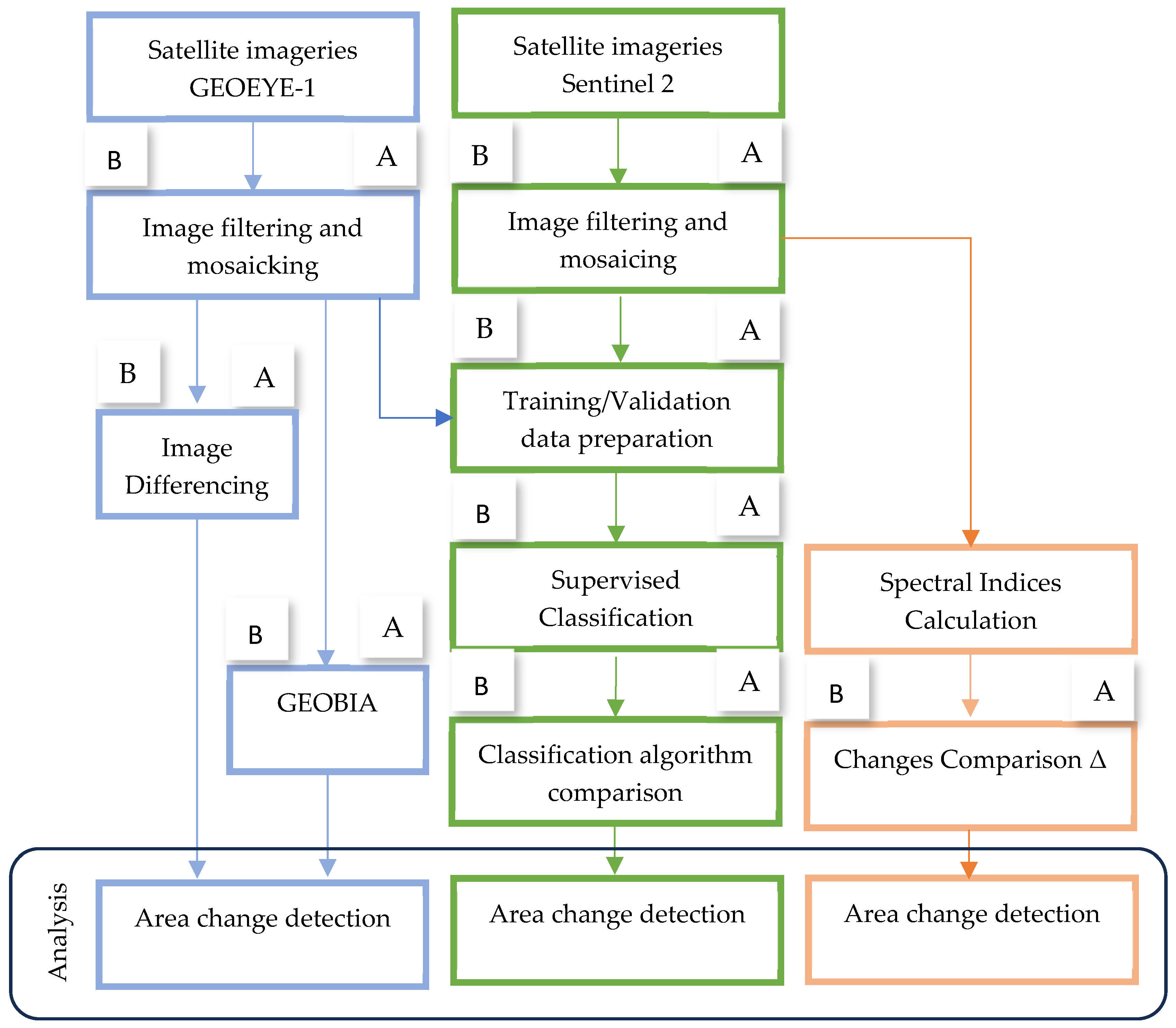
The primary goal of this study is to assess the capabilities of various remote sensing indices, algorithms, and datasets for detecting and quantifying qualitative and quantitative changes caused by the devastating flood in Derna, Libya, in September 2023. Specifically, the research focuses on determining the most effective indices and algorithms for post-flood change detection, exploring the contributions of different remote sensing datasets to the accuracy and reliability of flood impact assessments. By employing image classification-based change detection techniques, the study aims to identify specific land cover and hydrological changes while evaluating the strengths and limitations of these methods in comparison to other approaches. This integrated approach seeks to bridge methodological exploration with practical outcomes, offering valuable insights into the impact of the flood and the effectiveness of remote sensing tools in post-disaster analysis. The aim of this research is threefold. The first is to explore different image classification algorithms for change detection, including random forest [
76], classification and regression tree (CART) [
77], Naïve Bayes [
78], and support vector machine (SVM) [
79] algorithms. The second method estimates change detection using high-resolution remote sensing data and the image differencing method. The third is to develop an integrated measure for change estimation that will account for the outputs of different change detection methods. In addition, different indices (normalized difference vegetation index (NDVI) [
80], soil adjusted vegetation index (SAVI) [
81], transformed NDVI (TNDVI), and normalized difference moisture index (NDMI) [
82] were calculated using Multispectral Sentinel-2 images to facilitate the recognition of damaged regions by the changes in vegetation that were flashed away during the flood. The last objective of the study was to extract buildings using object-based image analysis (OBIA) and very high-resolution GEOEYE-1 images to quantify the buildings that collapsed due to floods.
The remainder of this paper is structured as follows.
Section 2 provides an overview of the study area and key features of the flood, its reasons, and its aftermath.
Section 3 deals with the description of remote sensing data used for analysis.
Section 4 presents a theoretical framework for change detection methods. A brief description of image differencing, spectral indices, post-classification, and geographic object-based image analysis are provided.
Section 5 details the findings of change detection research. This section outlines the results of image differencing change detection using high-resolution remote sensing data. The section then presents the results of post-classification change detection using different classification methods. The integrated measure for different layer change estimation is considered. The analysis concludes with calculation and comparison.
Section 5 furnishes the final output of the analysis of the detected changes.
Section 6 is dedicated to conclusions.
2. Study Area
Libya, situated in northern Africa, covers a vast expanse of 1,759,540 square kilometers and possesses a highly distinctive climate (
Figure 1). The country has an estimated population of around 7 million, according to the United Nations in 2021 [
83]. Indeed, Libya is characterized mainly by a desert climate, marked by summer temperatures often exceeding 40 degrees Celsius and relatively mild winters, with sporadic rainfall primarily concentrated in the winter months [
83]. Over 95% of the country’s land area lies below the 100 mm isohyet, classifying it as a hyper-arid zone, if not outright desert [
84]. However, the coastal regions in the west enjoy a Mediterranean climate with precipitation ranging between 300 and 500 mm per year. Occasionally, Mediterranean-level storms can take advantage of favorable meteorological conditions (such as elevated sea surface temperatures) to cause flooding in Europe and along the African coast. This pluviometric situation presents significant imperatives for water resource management and calls for adaptive solutions to ensure sustainable development in the country.
In September 2023, Storm Daniel formed above the Ionian Sea between Italy, Greece, and the Balkan Peninsula in the Mediterranean basin. Elevated temperatures during this season contributed to the necessary moisture production. The sea surface temperature of the Mediterranean was hot, surpassing the usual temperatures by two to three degrees and reaching a record of 28.71 °C in July. On 4 September, the storm moved inland, impacting the Balkans and bringing heavy rains to the region. The Greek National Meteorological Service officially named it, following the classification of European meteorological services. This event occurred during the European winter storm season of 2022–2023. Between 4 September 2023 and 7 September 2023, torrential precipitation led to severe flooding in Turkey, Greece, and Bulgaria, resulting in loss of human lives, with at least 26 reported deaths and 2 individuals still missing.
In the following days, the system moved southeastward, reaching its peak as a subtropical storm with recorded winds of 83 km/h, according to Meteorological Operational satellite (MetOp) instruments. On 10 September, Storm Daniel continued its trajectory eastward, penetrating further inland and eventually reaching the Northeast of Libya. There, it unleashed 414 mm of rain in a single day. The consequences were catastrophic: floods and mudslides, triggered by the collapse of the Derna dams, led to over 11,470 fatalities and left at least 10,000 individuals missing. Subsequently, the storm weakened and reached the North of Egypt on the 11th of September, causing moderate-level precipitation. Ultimately, it significantly diminished in intensity, transitioning into a residual depression due to the interaction of dry air and friction before eventually dissipating completely on 11 September 2023.
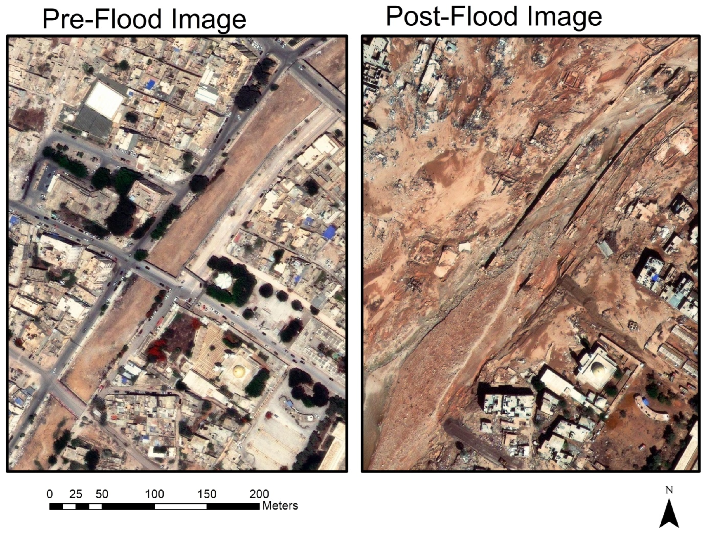
The most impacts of Storm Daniel’s flooding were concentrated in Libya, specifically in the port city of Derna, which has a population of approximately 90,000. The torrential rainfall of 414 mm led to the breach of the adjacent Derna and Abu Mansur dams, both around fifty years old. This allowed a flow more than 100 m wide to rush in, inundating the city’s heart along the Wadi Derma riverbed, which is typically dry for most of the year. Dwellings collapsed, resulting in both human and material losses. However, the breach of the second dam, located just one kilometer inland from Derna, released floodwaters measuring 3 to 7 m in height, submerging the city. Sudden floods destroyed roads and swept entire neighborhoods towards the sea (
Figure 2).
5. Results and Discussion
5.1. Image Differencing Change Detection
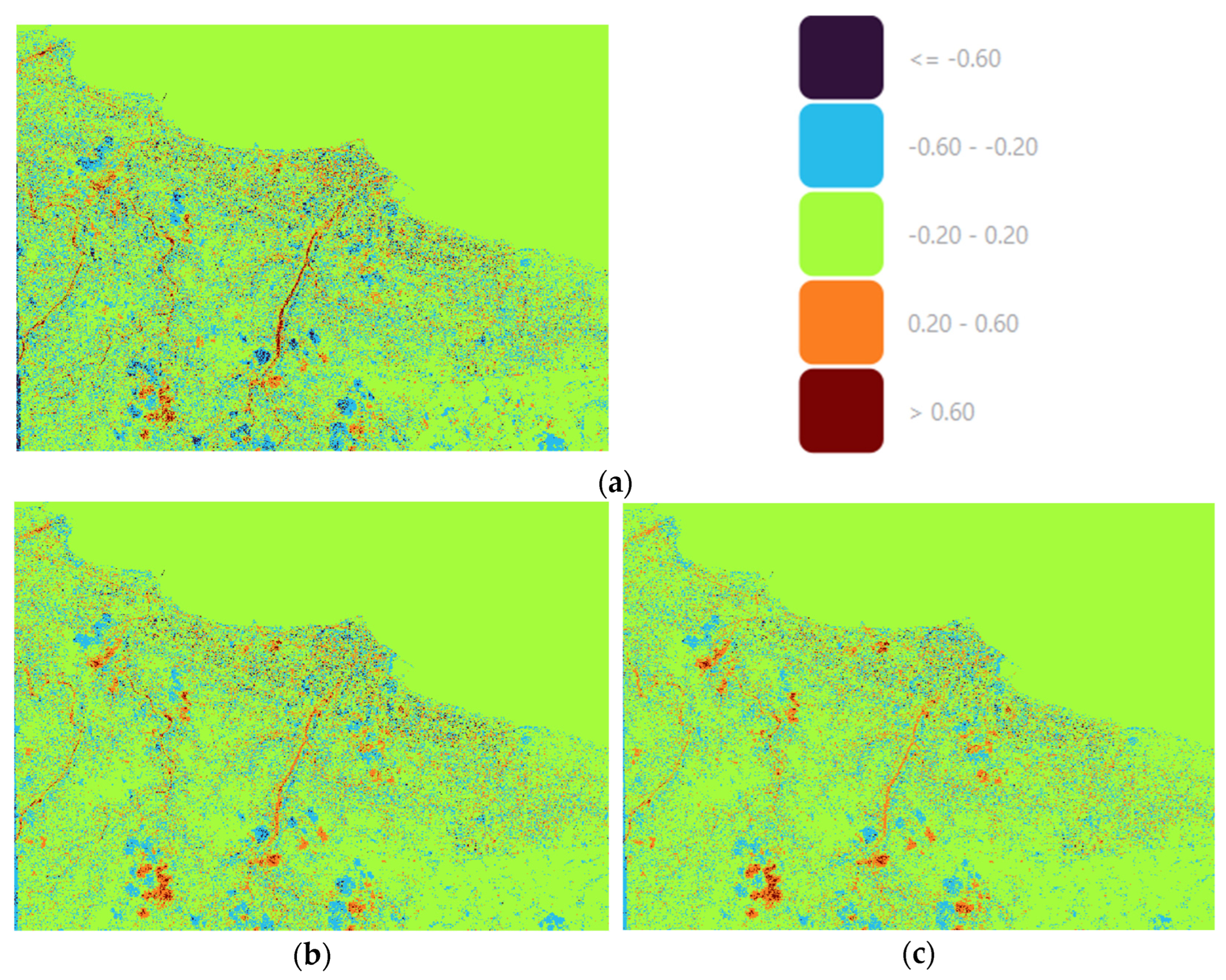
The image differencing method was applied to GEOEYE-1 images. Post-flood GEOEYE-1 images were georeferenced with pre-flood images to minimize the offset between two different time images in QGIS. Before differencing, every image was corrected for abnormal radiance deviations and normalized using standard image processing procedures in QGIS. In
Figure 4a,b, one may see the results of the image differencing procedure for the Derna testing region. The threshold values were accepted with an interval of 0.4 in a range from −1 to 1. The sea surface was excluded before further analysis. The regions that span values from −0.20 to 0.20 are accepted as having no changes. In the earlier explanation, a threshold value of 0.2 was proposed as a practical cut-off to distinguish between significant changes and noise. Here, the range from −0.20–0.20 effectively incorporates that threshold by treating radiance differences within this range as “no changes”. This approach aligns with the idea that radiance changes below the magnitude of 0.2 (whether positive or negative) are likely due to noise, minor environmental fluctuations, or preprocessing artifacts, rather than actual changes in the scene.
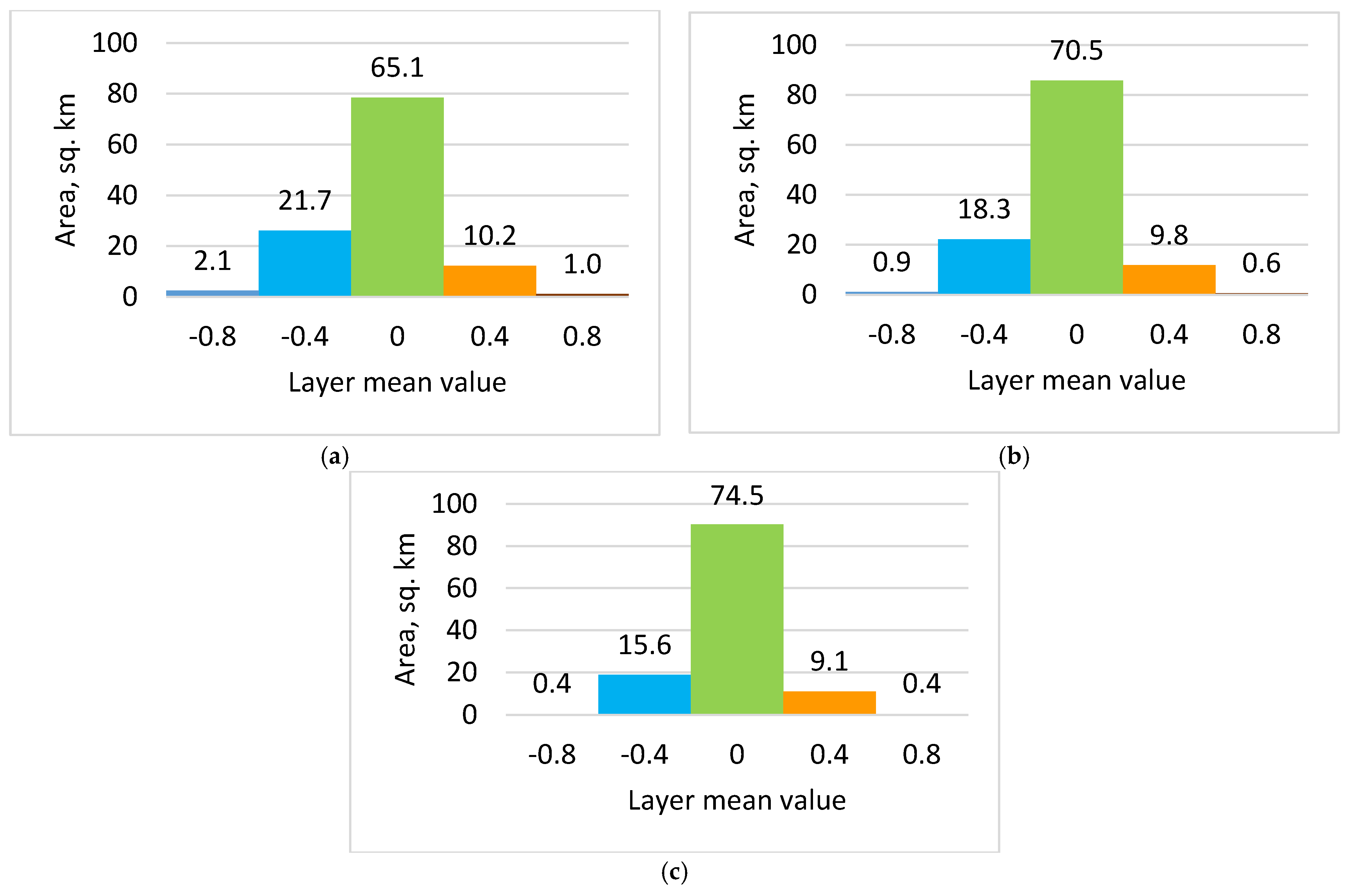
Figure 5a–c presents the area change histograms. The mean area of change exceeds 30%.
The image differencing approach gives a first glance at the degree of changes and allows us to estimate the approximate level of destruction.
5.2. Spectral Indices-Based Change Detection
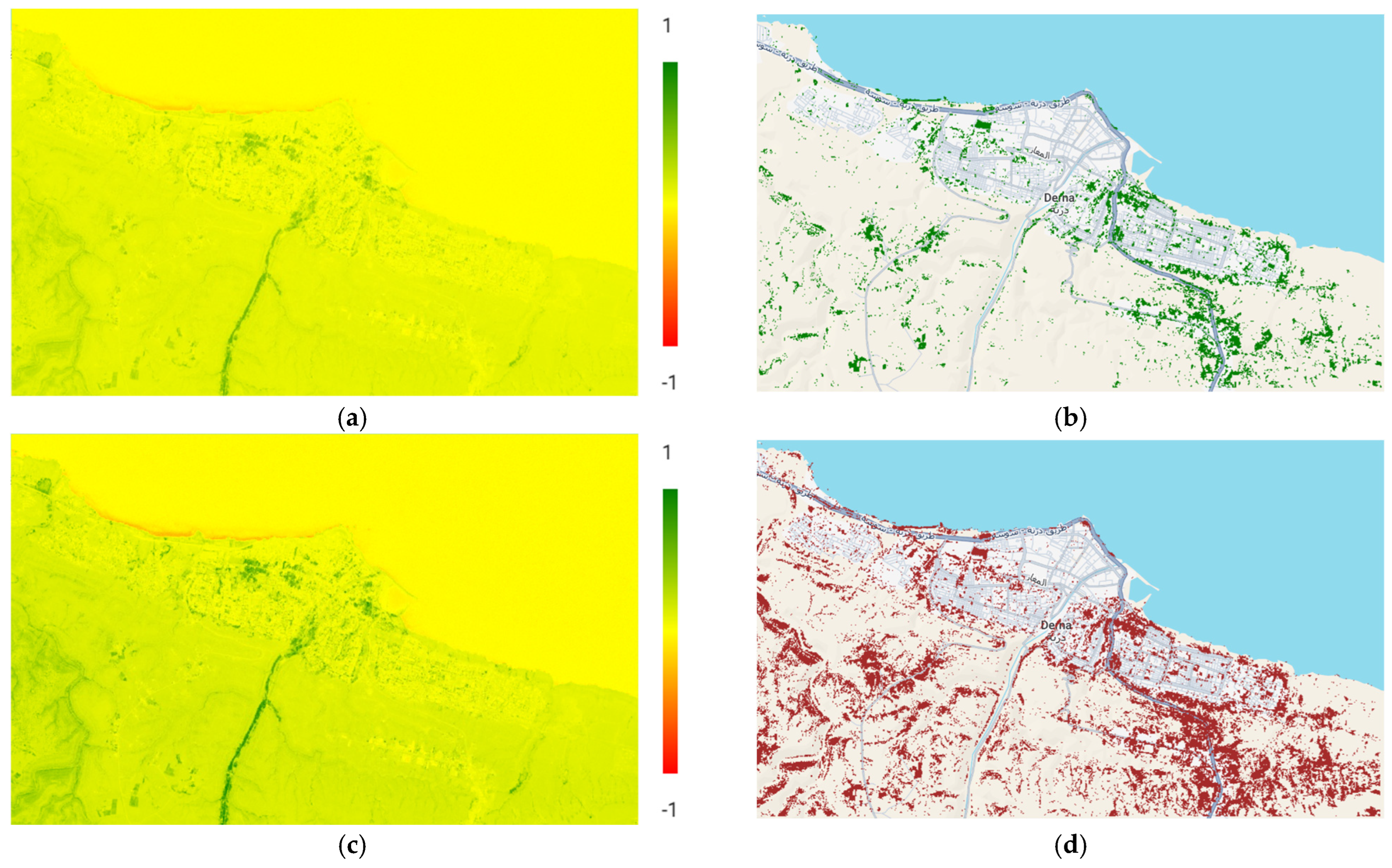
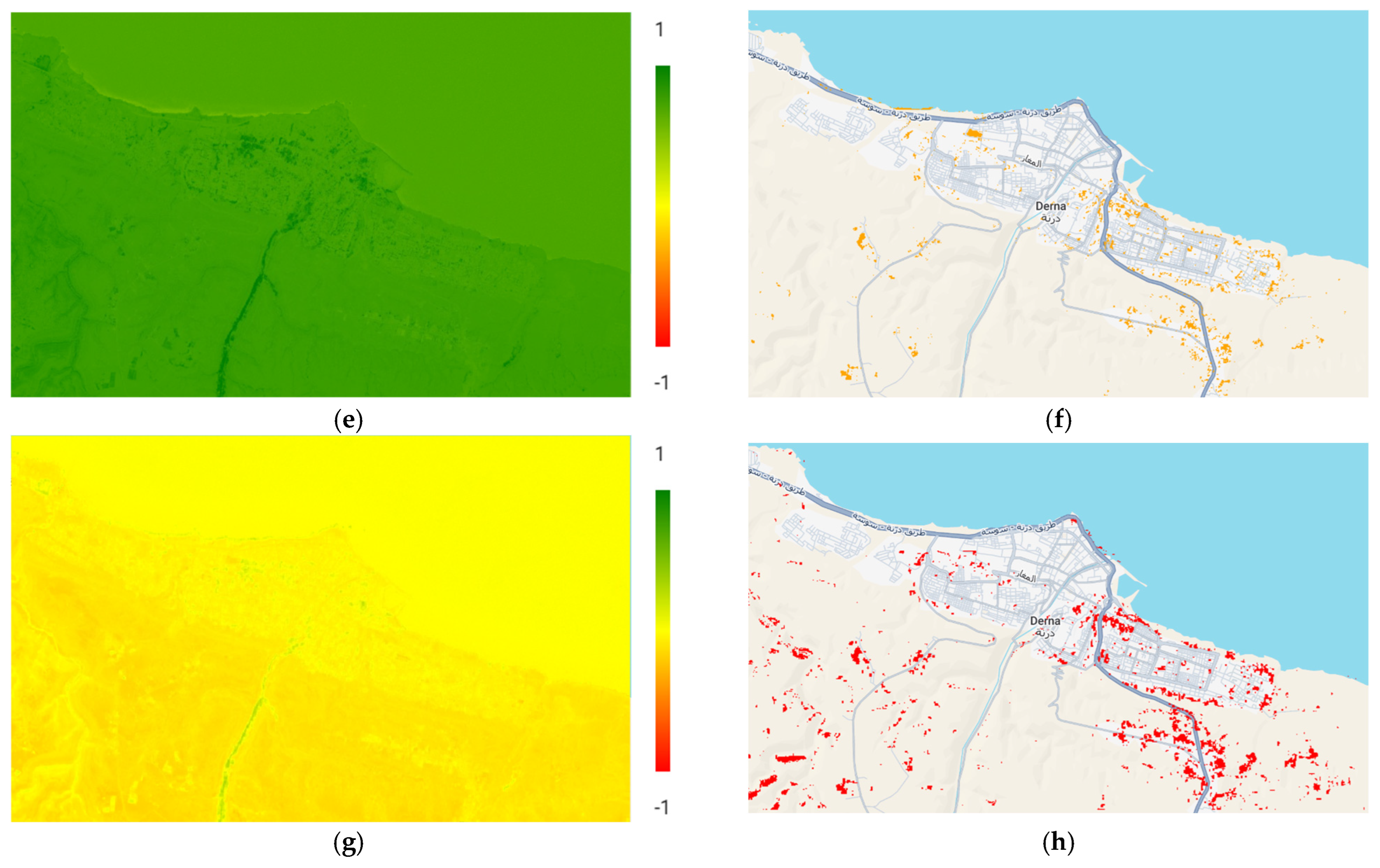
Spectral index is the most popular technique developed for image analysis. The first index used for the analysis is the traditional NDVI (4). The different values of NDVI correspond to water bodies (−1 to 0), barren rocks and sand (−0.1 to 0.1), sparse vegetation (shrubs, grasslands, or senescing crops, 0.2 to 0.5), and dense vegetation (0.6 to 1.0). The second index used for analysis is SAVI (5). The third is the TNDVI (6). This index shows the same sensitivity as SAVI to the optical properties of bare soil subjacent to the cover. Since we are dealing with flooded areas, the NDMI (7) is of interest. From its name, it is clear that this index can be used for monitoring vegetation, water, and drought. The values of NDMI are distributed in the following way: barren soil (−1), water stress (−0.2 to 0.4), and high canopy without water stress (0.4 to 1). For our case, the primary interest is not the indices’ values themselves but rather their changes between observation epochs. These changes will allow us to identify the ground transformation invoked by the flood, e.g., vegetated areas into barren or sand lands. To this end, the primary stress has been placed on the index differences converted into areas. The visual presentation of the differences calculated by Sentinel-2 images is given in
Figure 6, where the left images present the spectral indices before the flood (
Figure 6a,c,e,g), and the right images correspond to the differences of the spectral indices before and after the flood (
Figure 6b,d,f,h).
Based on the obtained differences, the changes in square kilometers were calculated (
Table 2).
Generally, indices differences describe the reasons for changes well. The issue is determining the types of objects that underwent the changes. To overcome this problem, the images must be previously classified, and appropriate changes must be determined based on class differences.
5.3. Classification Change Detection
Google Earth Engine was used as the primary tool for classification and further layer differencing using Sentinel-2. The classification algorithms considered were outlined in
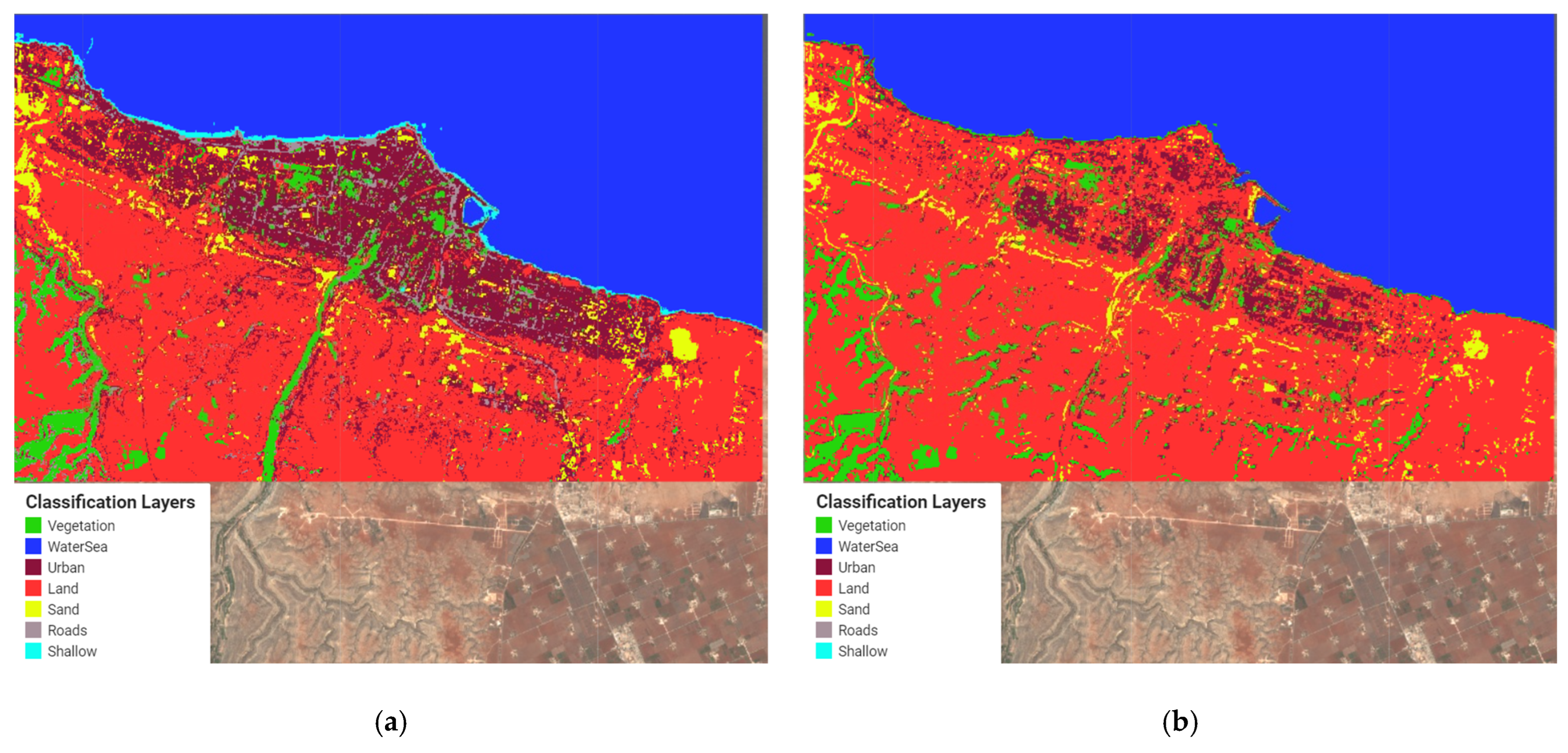
Section 4.3. The first tested algorithm was Smile Random Forest. The basic hyperparameter of the Smile Random Forest algorithm is the “number of trees”. The study explored three different values of “number of trees” (10, 100, and 300). The classification results before and after the flood are presented in
Figure 7.
Seven land cover classes were chosen for the classification: vegetation, urban territories, barren lands, sand, roads, shallow water, and water bodies. Forty points and twenty polygons of different sizes have been chosen for supervised learning in each class. Additionally, twenty points for each layer were collected for the classification estimation. The measurements allowed us to generate a confusion matrix for before and after flood classification. The classification accuracy for different classes was calculated using the figures from the confusion matrix (
Table 3).
Regardless of the accuracy obtained, the differences between respective classes were calculated. These differences were obtained in pixels and converted into square kilometers. Areas in square kilometers are presented in
Table 4.
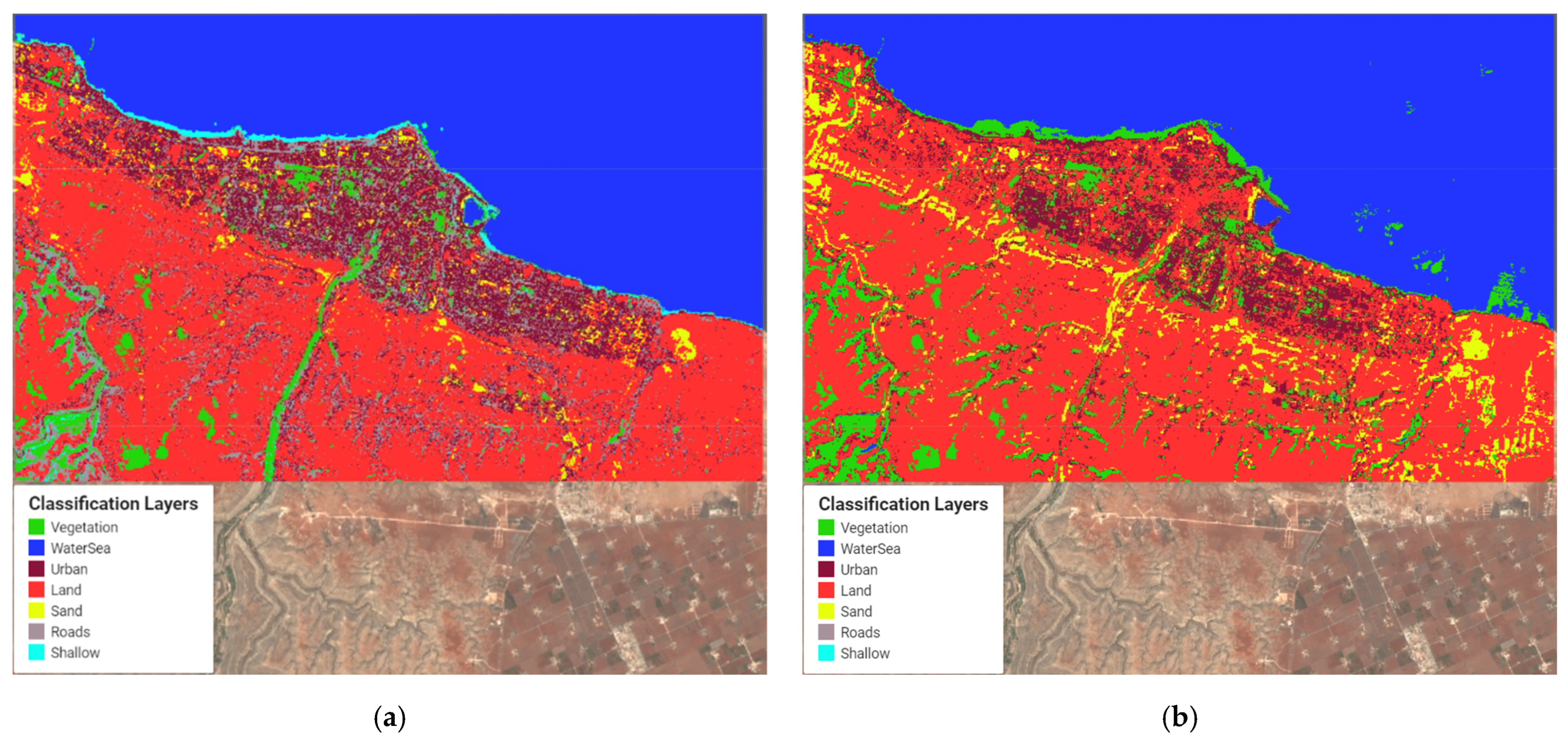
Figure 8a,b present the classification results for the CART algorithm. The hyperparameters for this algorithm are the maximum number of leaf nodes in each tree, which is by default assigned no limit, and the minimum leaf population, which is by default equal to 1.
Classification accuracy derived from the confusion matrix is outlined in
Table 5.
The differences between the respective classes are shown in
Table 6.
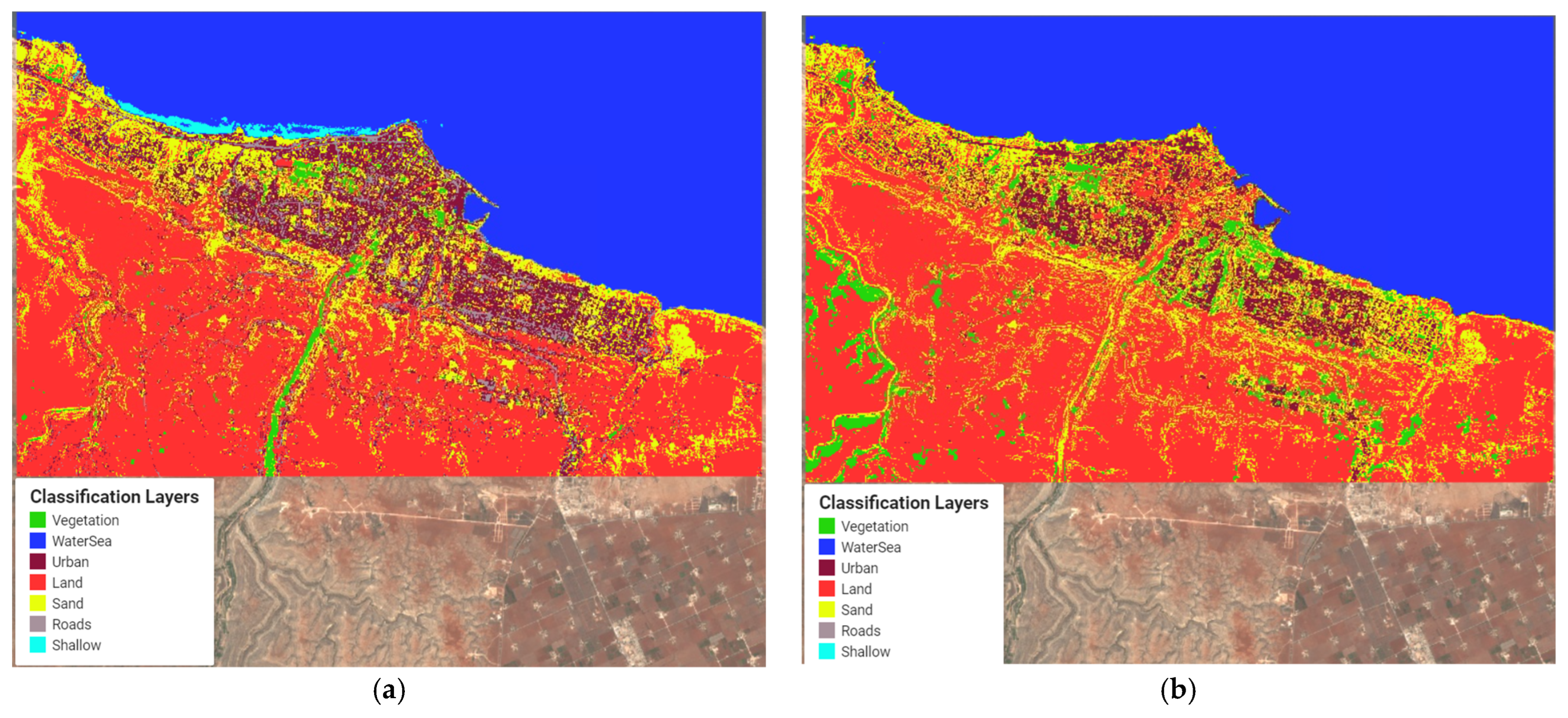
The third classification was accomplished by leveraging the Naïve Bayes algorithm. The Naïve Bayes algorithm has only one hyperparameter: the smoothing lambda coefficient, 0.000001. The classification results for the Naïve Bayes algorithm are presented in
Figure 9. Naïve Bayes performed poorly, highlighting its limitations in handling correlated and visually complex features, as seen in flood image classification, where spatial dependencies and complex patterns are crucial. Understanding these nuances is critical for selecting the most suitable model for specific classification tasks.
Classification accuracy is outlined in
Table 7.
The differences between respective layers are shown in
Table 8.
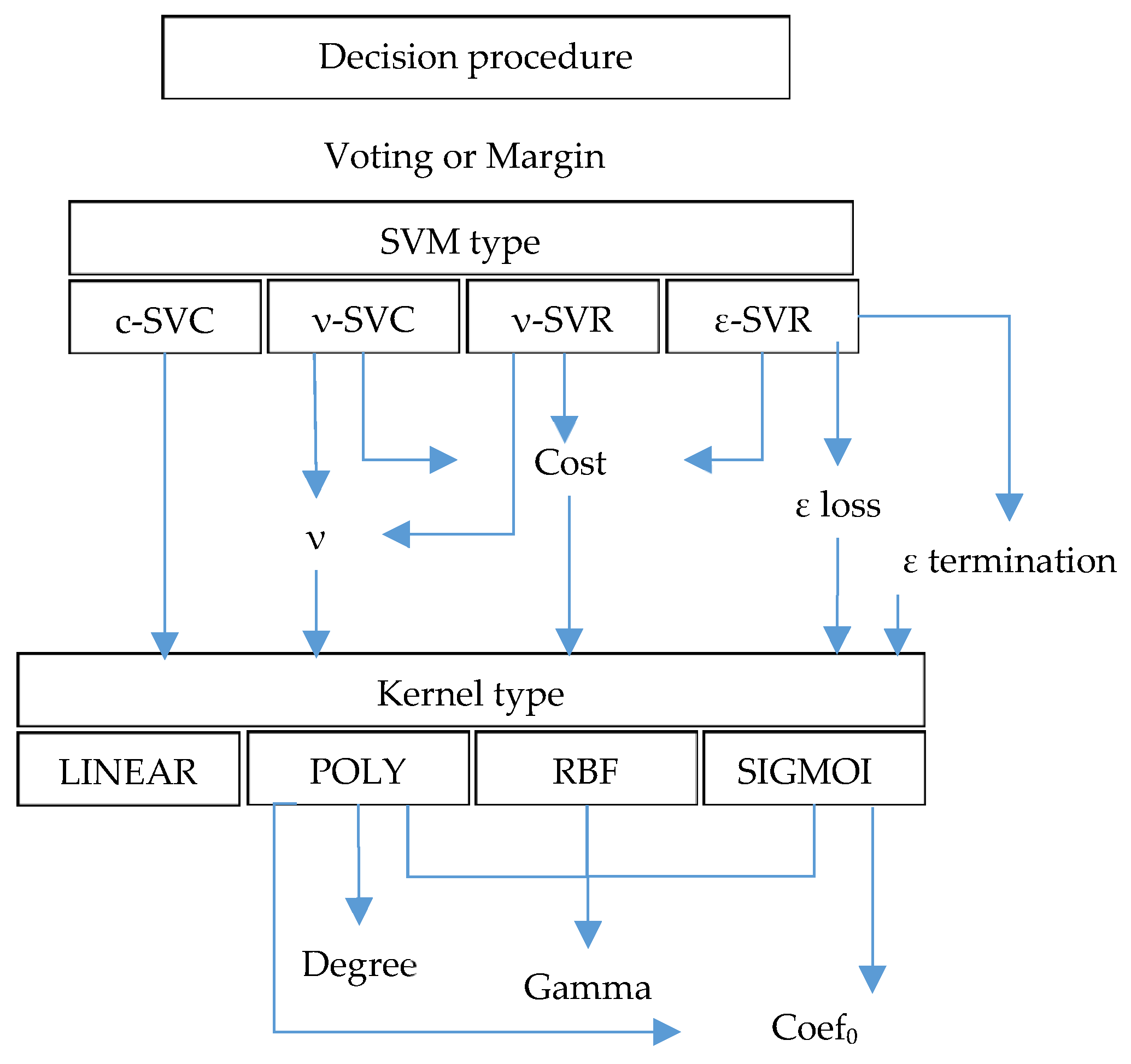
Unlike the others, the Support Vector Machine (SVM) algorithm has multiple hyperparameters. For convenience, we merged all possible ways and hyperparameters for SVM classification into the diagram in
Figure 10. Different sets of hyperparameters are possible depending on the SVM and kernel type. One may find the detailed description of the hyperparameters in Google Earth Engine documentation. Only specific SVM types fit well for classification tasks. The focus has been placed on SVM type c-SVC. The different kernels, namely LINEAR, POLY, RBF, and SIGMOID, were tested for this SVM type. The various degrees (two, three, and four) were considered for the polynomial kernel.
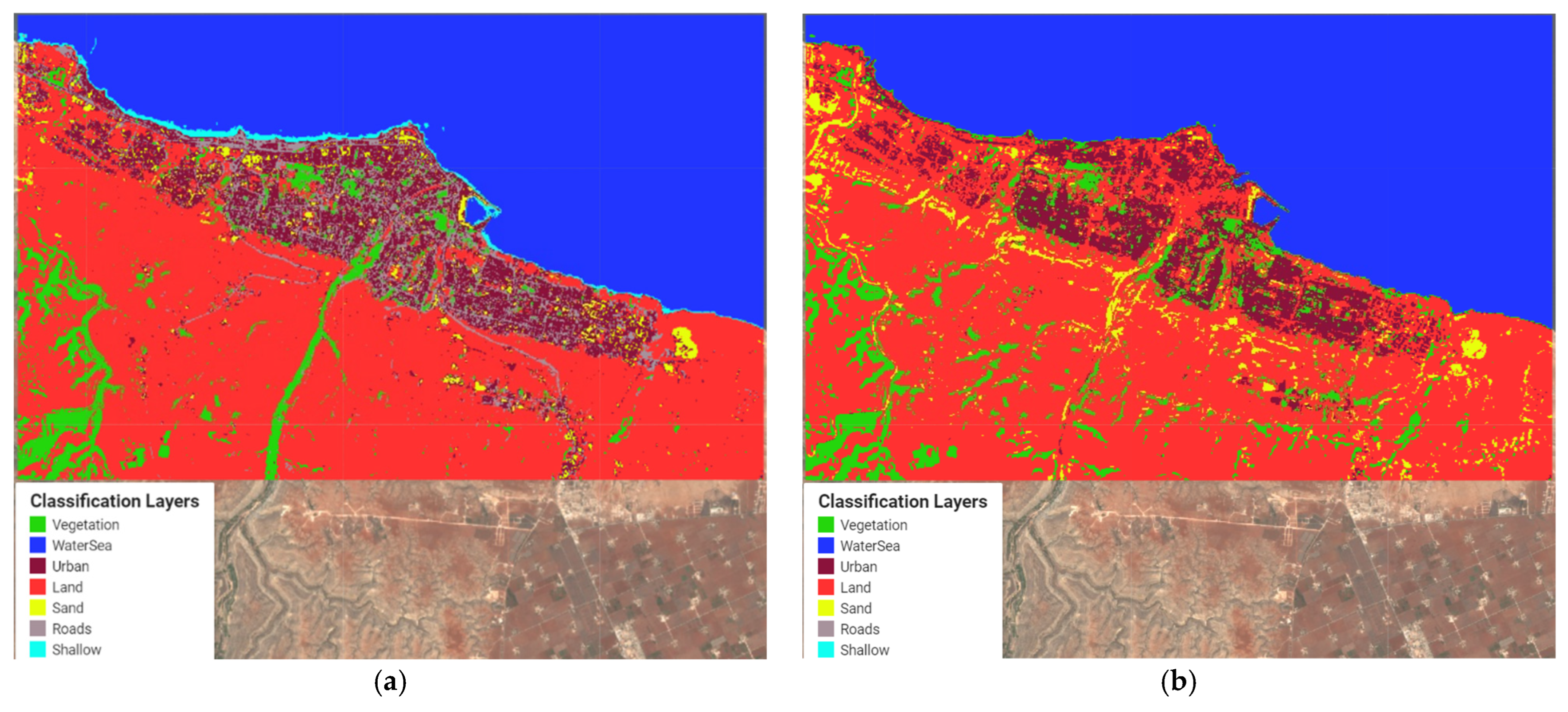
Below, we provided the results of two classifications. The first results correspond to the linear kernel case with other parameters assigned by default. The visual presentation is given in
Figure 11a,b. The second result is provided for the classification that ensured the highest accuracy. The classification was accomplished for the polynomial kernel with a degree of three (
Figure 12a,b).
Table 9 outlines classification accuracy derived from SVM classification, while
Table 10 shows classification accuracy for SVM with a polynomial kernel.
The differences between the respective layers are given in
Table 11 and
Table 12.
5.4. Integrated Estimation of Changes
Insofar as the different classification algorithms ensure different values, it is necessary to work out the estimate of the area change to account for the various accuracies of the algorithms. The integrated measure for different algorithms of area estimation is offered to calculate by the following expressions:
Mean value calculation for each layer over the different algorithms:
Control and elimination of the area estimations that exceed the value:
Weighted values calculation of the area changes before and after the flood:
where
.
First, we calculate mean values (15) over each region for the same classes. The deviations are calculated based on the mean values (16). If a particular deviation exceeds the value
then the area is considered an outlier and is ruled out from further analysis. The area changes for each layer are calculated using the producer’s accuracy as weights
. The results of this algorithm are given in
Table 13.
The integrated estimation of changes shows that the changes are mainly related to the transformation of urban territories to barren lands.
5.5. Geographic Object-Based Image Analysis
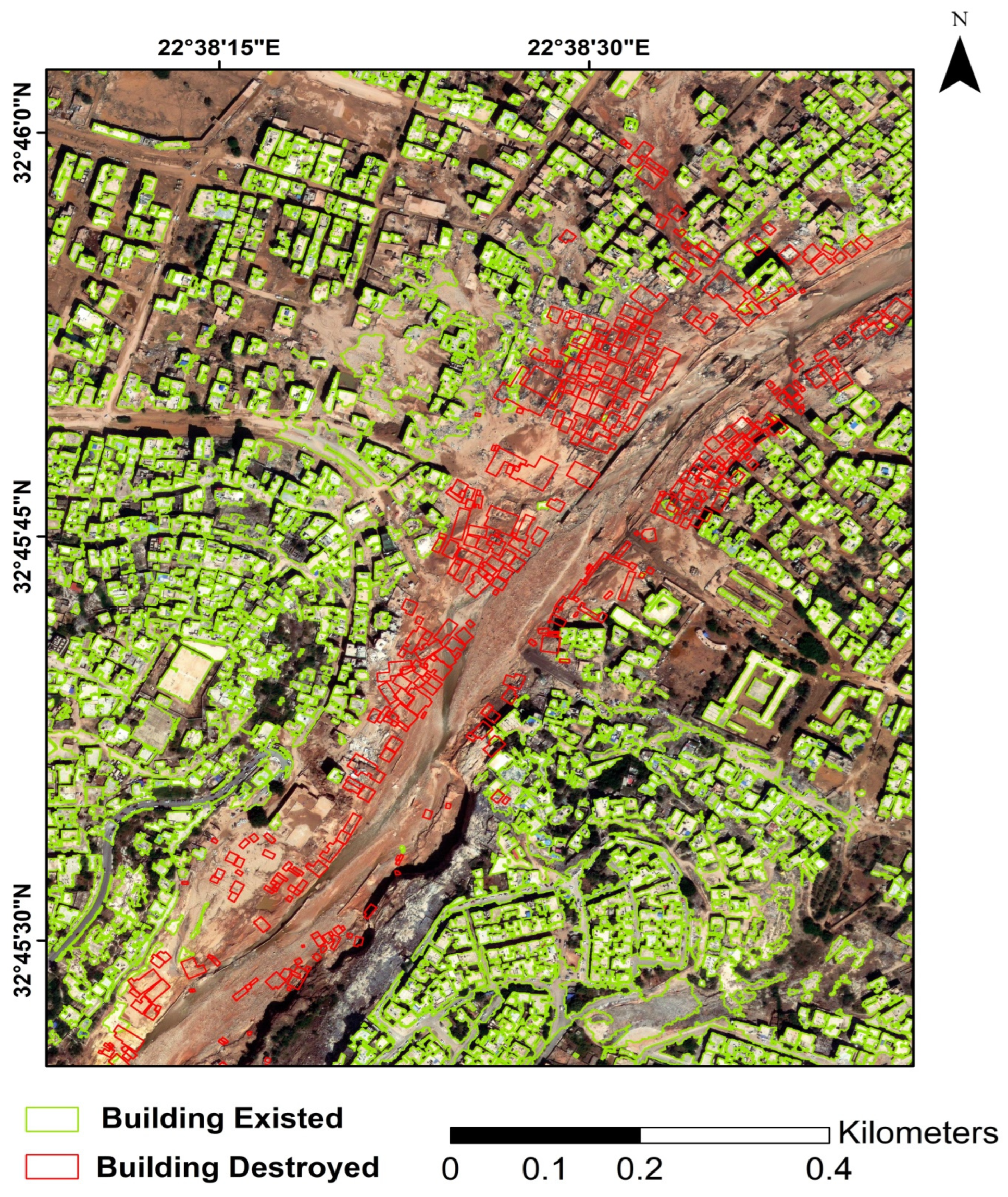
For this study, buildings were extracted from very high-resolution GEOEYE-1 data using Geographic Object-Based Image Analysis (GEOBIA). As we have only three band RGB images and no elevation information, our classification is based on only three bands with a spatial resolution of 0.5 m, which makes it suitable for detecting the shape of the rooftops. First, image objects were created using a multiresolution segmentation algorithm. This algorithm is bottom-up segmentation based on a pairwise region merging technique. Multiresolution segmentation is an optimization procedure that minimizes the average heterogeneity and maximizes their respective homogeneity for a given number of image objects. In multiresolution segmentation, we selected the optimum value of scale parameters according to the shape and size of buildings using a trial-and-error approach. After object creation, we use RGB bands to calculate different indices, such as brightness, blue-to-green, and blue-to-red ratios. We also used geometric features of rectangular fit and compactness. As a post-flood image has shadows, a blue band was used to separate shadows from other objects. A rule-set approach was used by incorporating different spectral, geometric, and contextual features for the classification of buildings. To further refine buildings, the relative border to shadow feature was used to classify building footprints accurately. Building footprints from post-flood images were compared with pre-flood building footprints to estimate the number of buildings that have been totally destroyed due to flash floods along the banks of the Derna River (
Figure 13). We compared the buildings extracted using the GEOBIA method against the high-resolution imagery and found that extracted buildings are in good agreement with the boundary of the buildings in high-resolution imagery, with an overall accuracy of 88%.
Figure 13 shows significant damage to critical infrastructure, including bridges, roads, and electricity grids, especially since most of the buildings were totally destroyed along the banks of the river. By comparing the buildings extracted using a post-flood image with pre-flood buildings, it was found that more than 600 buildings totally collapsed along the banks of the Derna River, in addition to major damage to buildings away from the banks of the Derna River.
5.6. Discussion
As indicated in the Introduction, the initial objective of the study was to explore the capabilities of different algorithms and remote sensing data processing strategies to estimate the flood aftermaths in northern Libya (Derna). The changes can be assessed in two different ways: by variations in spectral characteristics or by object detection algorithms. The correct estimation can be obtained only by combining these two approaches because the study region has urban and rural areas. Object detection algorithms will not provide adequate results for the rural areas’ lack of man-made objects. Therefore, we suggested a strategy for which we step-by-step make the change identification process more complex. We commence with simple image differencing, proceed with spectral indices and post-classification changes, and finish with object-based image analysis.
The first examined approach was image differencing. The differences were calculated for three spectral bands of GEOEYE-1 images. All spectral bands had similar differences. The normalized differences ranged from −1 to 1. Regardless of the difference sign, all values greater than 0.2 were treated as significant. The values lower than 0.2 were considered as measurement noise. Under such a premise, the mean changes reached 30%. It was unsurprising to see that the image differencing approach has low accuracy due to reasons mentioned in
Section 4. Another drawback is the impossibility of identifying the type of objects that changed their characteristics. Thus, we can recommend this approach for very tentative estimation.
Image differencing proved the existence of changes. To understand the object types that underwent the changes, we suggested accompanying the simple image differences with spectral index differences. Therefore, we selected four indices that might help us grasp the object types. This study found that NDVI changes corresponded to 4.6% of the study area. This finding was not unexpected since this index describes mainly vegetation changes, and the study region has very sparse vegetation. The detected changes may correspond to the transformation of some grasslands to barren lands of flood debris. The best estimation was obtained using the SAVI index. Insofar as SAVI describes barren lands, its change corresponds to debris spread throughout the study area. The total change was determined to be around 15% against 30% for the image differencing. These conflicting experimental results could be associated with the nature of the data. Image differencing is based on high-resolution images. However, the differences were determined for only three spectral bands, which is, in our opinion, considered unreliable. On the other hand, the spatial resolution of Sentinel-2 images is much lower, but the spectral is much better. Thus, the changes found by spectral indices for these data have better reliability since more spectral bands were included for calculation. The overlay of image differencing and SAVI changes showed the approximate coincidence of changes detected by these two methods.
To dive deeper into object identification and their changes, we suggested applying post-classification change detection. The first explored classification algorithm was Smile Random Forest. The classification accuracy before the flood was 0.94; after that, it was 0.89. The algorithm identified a significant change in land class around 10.3 sq. km, equivalent to 11.6%. The second algorithm was CART. CART ensured a lower classification accuracy: 0.89 before and 0.84 after. Such an accuracy level is critical, as most scientists recommend having it around 0.9–0.95. The changes in class areas are not distinct and vary in a range of +/−4–6 sq. km. The Naïve Bayes algorithm has even worse accuracy. Moreover, it is the only algorithm that has unclassified areas. The best accuracy was achieved by the support vector machine algorithm (SVM). SVM has a lot of hyperparameters. By tweaking these hyperparameters, the optimal combination is chosen, and the highest accuracy is ensured. In our case, the achieved pre-event classification accuracy was 0.94, and the post-event classification accuracy was 0.93. Contrary to expectations, the SVM did not find significant changes in the land class (3.5 sq. km). What is surprising is that changes in other classes were negligible. Different classification results pushed us to develop the integrated estimation of changes. This estimation uses classification accuracies as weights. Using this integrated estimation, we obtained the maximum changes for land class (+5.4%), road class (−3.5%), urban class (−2.6%), and vegetation class (+2.4%). The accumulation of flood debris explains the reduction of the road network and urban areas. Meanwhile, the growth of vegetation is related to the irrigation of flooded areas. The total absolute change is 17.5%, which corresponds well to the changes determined by spectral indices—roughly 15%. However, we now know the types of objects with appropriate, reliable accuracy.
At the final step of our strategy, we applied geographic object-based image analysis to explore the changes in urban areas. This algorithm works well for artificial objects with distinct structures and geometry. Of course, GEOBIA can be applied to natural objects, but the final results may be contradictory. So, once we determined the overall level of changes and object classes with the highest variability, we used GEOBIA to calculate the number of objects changed after the flood. As anticipated, the main changes happened in the central part of the city, where many buildings were washed away after the dam collapsed. GEOBIA allowed us to determine the number of totally destroyed buildings, which is equal to 600. Therefore, we obtained a quantitative estimation of the destruction level in addition to a qualitative assessment.
Returning to the question posed at the beginning of this paper, the suggested strategy can now be successfully applied to assess natural disaster aftermath using multi-temporal and multi-source data. As mentioned in the Introduction, flood studies using remote sensing data have become the most common tool for analysis. In this line, our analysis strategy demonstrates a higher flexibility compared to others. For earlier studies, e.g., [
23], the authors focused their attention on particularly water detection, which limits the study to one detectable class. Therefore, the aftermath estimation is problematic. Moreover, such studies are based on entirely optical bands that put forward additional conditions on object classification. A comparison of our findings with those of other studies [
31,
32] confirms that the existing works mostly stressed pre-flood analysis using remote sensing and GIS tools [
34,
35,
36,
37]. In contrast, our research and results deal with after-flood analysis. Generally speaking, the after-flood analysis can be referred to as a broader task known as change detection. According to this, the obtained result has not previously been described. The works [
42,
44,
50] consider solely object-based change detection; meanwhile, [
52,
54,
55] consider only one type of remote sensing data (visible or multispectral) for analysis. In light of this discussion, our approach is different since we fused different data (visible and multispectral bands) and various processing strategies (image differencing, object-based image analysis, image classification, and spectral indices) into one flowchart that made our results more reliable. Image differencing can be used for coarse estimation, as its results can be two times different from the actual destruction level. Spectral indices provide a more reliable analysis. However, choosing the correct index is not a trivial task. Post-classification change detection is recommended when we want to know which object classes fell under the changes. Finally, if we want to know the exact number of changed objects, it is recommended to use geographic object-based image analysis. Depending on the requirements for the final accuracy, we may use simple image differencing, spectral index, or more sophisticated image processing algorithms.


